Schrödingerisation based computationally stable algorithms for ill-posed problems in partial differential equations

Abstract

We introduce a simple and stable computational method for ill-posed partial differential equation (PDE) problems. The method is based on Schrödingerization, introduced in [S. Jin, N. Liu and Y. Yu, Phys. Rev. A, 108 (2023), 032603], which maps all linear PDEs into Schrödinger-type equations in one higher dimension, for quantum simulations of these PDEs. Although the original problem is ill-posed, the Schrödingerized equations are Hamiltonian systems and time-reversible, allowing stable computation both forward and backward in time. The original variable can be recovered by data from suitably chosen domain in the extended dimension. We will use the backward heat equation and the linear convection equation with imaginary wave speed as examples. Error analysis of these algorithms are conducted and verified numerically. The methods are applicable to both classical and quantum computers, and we also lay out quantum algorithms for these methods. Moreover, we introduce a smooth initialization for the Schrödingerized equation which will lead to essentially spectral accuracy for the approximation in the extended space, if a spectral method is used. Consequently, the extra qubits needed due to the extra dimension, if a qubit based quantum algorithm is used, for both well-posed and ill-posed problems, becomes almost $\log\log{1/\varepsilon}$ where $\varepsilon$ is the desired precision. This optimizes the complexity of the Schrödingerization based quantum algorithms for any non-unitary dynamical system introduced in [S. Jin, N. Liu and Y. Yu, Phys. Rev. A, 108 (2023), 032603].

Keywords: ill-posed problems, backward heat equation, Schrödingerisation, quantum algorithms

1 Introduction

In this paper, we are interested in numerically computing ill-posed problems that follow the evolution of a general dynamical system

$$\frac{\mathrm{d}}{\mathrm{d}t}{\bm{u}}=H{\bm{u}},\quad{\bm{u}}(0)={\bm{u}}_{0}.$$ (1.1)

For simplicity, we first consider $H$ being Hermitian with $n$ real eigenvalues, ordered as

$$\lambda_{1}(H)\leq\lambda_{2}(H)\leq\cdots\lambda_{n}(H),\quad\text{for}\;\text{all}\;t\in[0,T].$$ (1.2)

We assume that $\lambda_{i}(H)>0$, for some $0\leq i\leq n$, which implies that the system contains unstable modes, thus the initial value problem is ill-posed since its solution will grow exponentially in time. This causes significant computational challenges. Normally the numerical errors will grow exponentially unless special care is taken.

Ill-posed or unstable problems appear in many physical applications, for example fluid dynamics instabilities such as Rayleigh-Taylor and Kevin-Helmholtz instabilities [16, 6], plasma instability [8], and Maxwell equations with negative index of refraction [24, 22]. It also appears in inverse problems [28, 2]. One of the most classical ill-posed problems is the backward heat equation which suffers from the catastrophic Hardmard instability. Usually some regularization technique is used to make the problems well-posed [4].

In this paper we study a generic yet simple computational strategy to numerically compute ill-posed problems based on Schrödingerization, introduced for quantum simulation for dynamical systems whose evolution operator is non-unitary [12, 13]. The idea is to map it to one higher dimensions, into Schrödinger-type equations, that obeys unitary dynamics and thereby naturally fitting for quantum simulation. Since the Schrödinger-type equations are Hamiltonian systems that are time-reversible, they can be solved both forwards and backwards in time in a computationally stable way. This makes it suitable for solving unstable problems, as was proposed in our previous work [11]. In this article we study this method for the classical backward heat equation, and a linear convection equation with imaginary wave speed (or negative index of refraction).

The initial-value problem to the backward heat equation is ill-posed in all three ways: (i) the solution does not necessarily exist; (ii) if the solution exists, it is not necessarily unique; (iii) there is no continuous dependence of the solution on arbitrary input data [21, 14, 9, 18]. This problem is well-posed for final data whose Fourier spectrum has compact support [20]. However, even when the solution exists and is unique, computing the solution is difficult since unstable physical systems usually lead to unstable numerical methods. There have been various treatments of this difficult problem, for example quasi-reversibility methods [29, 26, 17, 1, 19], regularization methods [7, 15, 26, 3], Fourier truncation methods [23], etc. Our approach computes solution consistent with the Fourier truncation method.

The actual implementation of our backward heat equation solver is as follows. First we start with the Fourier transform of the input data denoted by $u_{T}$ and truncate the Fourier mode in finite domain. This is either achieved automatically if the Fourier mode of $u_{T}$ has compact support, or we choose a sufficiently large domain in the Fourier space such that outside it the Fourier coefficient of $u_{T}$ is sufficiently small. The latter can usually be done since the forward heat equation gives a solution that is smooth for $t>0$ so its Fourier coefficient decays rapidly. The Schrödingerization technique lifts the backward heat equation to a Schrödinger equation in one higher dimension that is time reversible, which can be solved backward in time by any reasonable stable numerical approximation. We then recover $u(t)$ for $0\leq t<T$ by integrating or pointwise evaluation over suitably chosen domain in the extended variable. Since the time evolution is based on solving the Schrödinger equation, the computational method is stable.

We point out that the truncation in the Fourier space regularizes the original ill-posed problem. Although the initial-value problem to the Schrödingerized equation is well-posed even without this Fourier truncation, to recover $u$ one needs finite Fourier mode.

We will also apply the same strategy to solve the unstable linear convection equation that has imaginary wave speed.

We will give error estimates on these methods and conduct numerical methods that verify the results of the error analysis. The methods work for both classical and quantum computers. Since the original Schrödingerization method was introduced for quantum simulation of general PDEs, we will also give the quantum implementation of the computational method.

Moreover, we introduce a smooth initialization for the Schrödingerized equation, so the initial data will be in $C^{k}(\mathbb{R})$ in the extended space for any integer $k\geq 1$ (see Section 4.3). This will lead to essentially the spectral accuracy for the approximation in the extended space, if a spectral method is used. Consequently, the extra qubits needed due to the extra dimension, if a qubit based quantum algorithm is used, for both well-posed and ill-posed problems, becomes almost $\log\log{1/\varepsilon}$ where $\varepsilon$ is the desired precision. This optimizes the complexity of Schrödingerization based quantum algorithms introduced in [12, 13] for any non-unitary dynamical system.

The rest of the paper is organized as follows. In Section 2, we give a brief review of the Schrödingerization approach for general linear ODEs. In Section 3, we introduce the backward heat equation and show the approximate solution based on the framework of Schrödingerization. In Section 4, the numerical method and error analysis of the backward heat equation are presented. In addition, a $C^{k}$ smooth initial data with respect to the extended variable is constructed to improve the convergence rates in the extended space. In Section 5, we apply this technique to the convection equations with purely imaginary wave speed. In Section 6, we show the numerical tests to verify our theories.

Throughout the paper, we restrict the simulation to a finite time interval $t\in[0,T]$. The notation $f\lesssim g$ stands for $f\leq Cg$ where $C$ is independent of the mesh size. Moreover, we use a 0-based indexing, i.e. $j=\{0,1,\cdots,N-1\}$, or $j\in[N]$, and ${\bm{e}}_{j}^{(N)}\in\mathbb{R}^{N}$, denotes a vector with the $j$-th component being $1$ and others $0$. We shall denote the identity matrix and null matrix by $I$ and 0, respectively, and the dimensions of these matrices should be clear from the context, otherwise, the notation $I_{N}$ stands for the $N$-dimensional identity matrix.

2 The general framework

We start with the basic framework set up in [11] which we first briefly review here.

Using the warped phase transformation ${\bm{w}}(t,p)=e^{-p}{\bm{u}}$ for $p>0$ and symmetrically extending the initial data to $p<0$, one has the following system of linear convection equations [12, 13]:

$$\frac{\mathrm{d}}{\mathrm{d}t}{\bm{w}}=-H\partial_{p}{\bm{w}}\quad{\bm{w}}(0)=e^{-|p|}{\bm{u}}_{0}.$$ (2.1)

This is clearly a hyperbolic system. When the eigenvalues of $H$ are all negative, the convection term of (2.1) corresponds to waves moving from the right to the left. One does, however, need a boundary condition on the right hand side. Since ${\bm{w}}$ decays exponentially in $p$, one just needs to select $p=p^{*}$ large enough, so $w$ at this point is essentially zero and a zero incoming boundary condition can be used at $p=p^{*}$. Then ${\bm{u}}$ can be recovered via

$${\bm{u}}(t)=\int_{0}^{p^{*}}w(t,p)\,dp$$ (2.2)

or

$${\bm{u}}(t)=e^{p}w(t,p)\qquad{\text{ for any}}\quad 0<p<p^{*}.$$ (2.3)

However, when $\lambda_{i}(H)>0$ for some $i$, then some of these waves evolving via (2.1) will instead move from the left to the right. These are spurious waves that will pollute part of $p>0$ region so one cannot recover ${\bm{u}}$ from (2.2) or (2.3). In this case, one needs to use the following theorem [11].

Theorem 2.1.

Assume the eigenvalues of $H$ satisfy (1.2), then the solution of (1.2) can be recovered by

$${\bm{u}}(t)=e^{p}{\bm{w}}(t,p),\quad\text{for}\;\text{any}\;p\geq p^{\Diamond},$$ (2.4)

where $p^{\Diamond}\geq\max\{\lambda_{n}(H)t,0\}$, or recovered by using the integration,

$${\bm{u}}(t)=e^{p}\int_{p}^{\infty}{\bm{w}}(t,q)\;\mathrm{d}q,\quad p\geq p^{\Diamond}.$$ (2.5)

Since (2.1) is a hyperbolic system, thus the initial value problem is well-posed and one can solve it numerically in a stable way (as long as suitable numerical stability condition–the CFL condition–is satisfied). Thus although the original system (1.2) is ill-posed, we can still solve the well-posed problem (2.1), and then recover ${\bm{u}}$ using Theorem (2.1), as long as $\lambda_{n}(H)<\infty$!

We also point out that the extension to the $p<0$ domain is for the convenience of using the Fourier spectral method, which needs periodic boundary condition. The discretization of the $p$-derivative in (2.1) can be done using other numerical methods, for example the finite difference and finite element methods. In such cases one can just solve the problem in $p>0$ and, if $\lambda_{i}(H)>0$ for some $i$, one needs to supply boundary condition at $p=0$. This boundary condition can be set arbitrarily, since the induced spurious wave will propagate just with speed $\lambda_{i}(H)>0$, thus the recovering strategy given by Theorem 2.1 remains valid.

3 The backward heat equation

In this section, we consider the following one-dimensional backward heat equation in the infinite domain,

$$\partial_{t}u =\partial_{xx}u\;\,\quad\;\text{in}\;\Omega_{x}\quad 0\leq t<T,$$ (3.1)

$$u(T,x) =u_{T}(x)\quad\;\text{in}\;\Omega_{x},$$

where $\Omega_{x}=(-\infty,\infty)$. We want to determine $u(\cdot,t)$ for $0\leq t<T$ from the data $u_{T}$. The change of variable $v(t,x)=u(T-t,x)$ leads to the following formulation of (3.1),

$$\partial_{t}v =-\partial_{xx}v\;\,\quad\; \text{in}\;\Omega_{x}\quad 0\leq t<T,$$

$$v(0,x) =u_{T}(x)\quad\; \text{in}\;\Omega_{x},$$

The spatial discretization on $x$ by finite difference methods leads to Eq.(1.2) with all of the eigenvalues of $H$ being positive. Let $\hat{g}(\eta)$ denote the Fourier transform of $g(x)\in L^{2}(\Omega_{x})$ and define it by

$$\hat{g}(\eta):=\mathscr{F}(g)=\frac{1}{2\pi}\int_{\mathbb{R}}e^{ix\eta}g(x)\mathrm{d}x,\qquad g(x):=\mathscr{F}^{-1}(\hat{g})=\int_{\mathbb{R}}e^{-ix\eta}\hat{g}(\eta)\mathrm{d}\eta.$$

Let $\|g\|_{H^{s}(\Omega_{x})}$ denote the Sobolev norm $H^{s}(\Omega_{x})$ defined as

$$\|g\|_{H^{s}(\Omega_{x})}:=\big{(}\int_{\mathbb{R}}|\hat{g}(\eta)|^{2}(1+\eta^{2})^{s}\;\mathrm{d}\eta\big{)}^{\frac{1}{2}}.$$

When $s=0$, $\|\cdot\|_{H^{0}(\Omega_{x})}$ denotes the $L^{2}(\Omega_{x})$-norm. If the solution of (3.1) in this Sobolev space exists, then it must be unique [5]. We assume $u(t,x)$ is the unique solution of (3.1). Applying the Fourier transform, one gets the exact solution $u(t,x)$ of problem (3.1):

$$u(t,x)=\int_{\mathbb{R}}e^{-ix\eta}e^{\eta^{2}(T-t)}\hat{u}_{T}\;\mathrm{d}\eta.$$ (3.2)

For the above solution to be well-defined, we assume that $\hat{u}_{T}\in H^{s}_{0}$, namely $H^{s}$ with compact support. This yields a well-posed problem in the sense of Hardmard [20]. For more general $\hat{u}_{T}$ we will truncate the domain in $\eta$ and begin with the truncated–thus compactly supported–final data. Denoting $u_{0}(x)=u(x,0)$, then it is easy to see from (3.2) that

$$\|u_{0}\|_{H^{s}(\Omega_{x})}=\big{(}\int_{\mathbb{R}}|\hat{u}_{0}|^{2}(1+\eta^{2})^{s}\;d\eta\big{)}^{1/2}<\infty,\quad\text{for}\;s\geq 1.$$ (3.3)

The Schrödingerization for (3.1) gives

$$\frac{\mathrm{d}}{\mathrm{d}t}w =-\partial_{xxp}w\;\;\quad\quad\text{in}\;\Omega_{x}\times\Omega_{p}\quad 0\leq t<T,$$ (3.4)

$$w(T) =e^{-|p|}u_{T}(x)\;\;\quad\text{in}\;\Omega_{x}\times\Omega_{p},$$

where $\Omega_{p}=(-\infty,\infty)$. Following the proof in [5, Theorem 5, Section 7.3], one has $w(0,x,p)\in H^{s}(\Omega_{x})\times H^{1}(\Omega_{p})$ under the assumption  (3.3).

Again using the Fourier transform technique to (3.4) with respect to the variables $p$ and $x$, one gets the Fourier transform $\hat{w}(t,\eta,\xi)$ of the exact solution $w(t,x,p)$ of problem (3.4) satisfying

$$\frac{\mathrm{d}}{\mathrm{d}t}\hat{w}=-i\xi\eta^{2}\hat{w},\quad\hat{w}(T)=\hat{w}_{T}=\frac{1}{2\pi}\int_{\mathbb{R}}\frac{e^{-ix\eta}u_{T}(x)}{\pi(1+\xi^{2})}\;\mathrm{d}x=\frac{\hat{u}_{T}(\eta)}{\pi(1+\xi^{2})}.$$ (3.5)

The solution of $w$ is then found to be

$$w(t,x,p)=\int_{\mathbb{R}}\int_{\mathbb{R}}e^{-i(x\eta+p\xi)}e^{-i\xi\eta^{2}(t-T)}\hat{w}_{T}\;\mathrm{d}\eta\mathrm{d}\xi=\int_{\mathbb{R}}e^{-|p+\eta^{2}(t-T)|}\hat{u}_{T}(\eta)e^{-ix\eta}\;\mathrm{d}\eta,$$ (3.6)

and it is easy to check $w(t,x,p)\in H^{s}(\Omega_{x})\times H^{1}(\Omega_{p})$ from (3.6). Note the initial-value problem (3.4) is well-posed, even for $u_{T}\in H^{s}$ not being compactly supported in the Fourier space, as can be easily seen from (3.5), which is an oscillatory ODE with purely imaginary spectra.

By using the Fourier transform on $x$ gives

$$\partial_{t}\tilde{w}-\eta^{2}\partial_{p}\tilde{w}=0\quad 0\leq t<T,\quad\tilde{w}(T)=e^{-|p|}\hat{u}_{T},$$ (3.7)

where $\tilde{w}$ is the Fourier transform of $w$ on the $x$-variable. Here $\tilde{w}$ is a linear wave moving to the right, if one starts from $t=T$ and going backwards in time (one can also use the change of variable $t\mapsto T-t$ to make the problem (3.4) forward in time for notation comfort). This corresponds to the case of (2.1) in which all eigenvalues of $H$ are positive. Hence to recover $u$ one needs to use $p^{\diamond}>\eta^{2}T$ for time $T>0$. This is the basis for the introduction of our stable computational method: we solve the $w$-equation (3.4) with a suitable–stable– computational method, and then recover $u$ by either integration or pointwise evaluation using Theorem 2.1.

To proceed we will need to make some assumptions. In the continuous space $\eta$ maybe unbounded, thus the condition $p^{\diamond}>\eta^{2}T$ may not be satisfied. We consider two scenarios here:

1. $\hat{u}_{T}$ has compact support, namely $\hat{u}_{T}=0$ for $|\eta|>\eta_{\max}$ for some $\eta_{\max}<\infty$. While this is not generally true, when $u_{T}(x)$ is smooth in $x$, its Fourier mode decays rapidly, so one can truncate $\eta$ for $|\eta|>\eta_{\max}$ with desired accuracy.

2. One discretizes equation (3.4) numerically. This usually requires first to truncate the $x$-domain so it is finite, followed by some numerical discretization of the $x-$derivative, for example the finite difference or spectral method. Then $|\eta|\leq\eta_{\max}\leq\mathscr{O}(1/(\Delta x)^{2})$ where $\Delta x$ is the spatial mesh size in $x$.

For how to choose $\eta_{\max}$, see Remark 3.2.

We start by choosing an $\eta_{\max}>0$ and denote

$$\delta(\eta_{\max})=\big{(}\int_{\eta_{\max}}^{\infty}(1+\eta^{2})^{s}|\hat{u}_{0}|^{2}\;\mathrm{d}\eta\big{)}^{\frac{1}{2}}$$ (3.8)

to be a small quantity, which will be chosen with other error terms to meet the numerical tolerance requirement (see Remark 3.1). We define the ”approximate” solution $u_{\eta_{\max}}$ of (3.1) as follows:

Definition 3.1.

First, define

$$w_{\eta_{\max}}=\int_{\mathbb{R}}e^{-|p+\eta^{2}(t-T)|}\hat{u}_{T}(\eta)\chi_{\max}e^{-ix\eta}\;\mathrm{d}\eta,$$ (3.9)

where $\chi_{\max}(\eta)=1$ when $\eta\in[-\eta_{\max},\eta_{\max}]$, otherwise $\chi(\eta)=0$. Then one obtains the approximate solution $u_{\eta_{\max}}$ by

$$u_{\eta_{\max}}(t,x,p)=e^{p}w_{\eta_{\max}}(t,x,p),\quad\text{or}\quad u_{\eta_{\max}}(t,x,p)=e^{p}\int_{p}^{\infty}w(t,x,q)\;\mathrm{d}q,\quad p>p^{\Diamond},$$ (3.10)

with $p^{\Diamond}=\eta_{\max}^{2}T$.

With $u$ defined as above, we have the following theorem which gives an error estimate to the above approximation.

Theorem 3.1.

Suppose $\|u_{0}\|_{H^{s}(\Omega_{x})}$ is bounded, namely (3.3) holds. Let $u(t)=u(t,x)$ be the solution (3.1) given by (3.2), and $u_{\eta_{\max}}(t)=u_{\eta_{\max}}(t,x,p)$ given by (3.10) with $p>p^{\Diamond}=\eta_{\max}^{2}T$ and $\eta_{\max}$ chosen to satisfy (3.8). Then for any $p>p^{\Diamond}$, $t\in[0,T)$,

$$\|u(t)-u_{\eta_{\max}}(t)\|_{L^{2}(\Omega_{x})}\leq e^{-\eta_{\max}^{2}t}\delta/\eta_{\max}^{s}.$$ (3.11)

Proof.

According to Parseval’s equality and (3.2), (3.10), it follows that

$$\|u-u_{\eta_{\max}}\|_{L^{2}(\Omega_{x})} =\|\hat{u}-\hat{u}_{\eta_{\max}}\|_{L^{2}(\Omega_{\eta})}=\|e^{\eta^{2}(T-t)}\hat{u}_{T}-e^{\eta^{2}(T-t)}\hat{u}_{T}\chi_{\max}\|_{L^{2}(\Omega_{\eta})}$$

$$=\left(\int_{|\eta|>\eta_{\max}}|e^{\eta^{2}(T-t)}e^{-\eta^{2}T}\hat{u}_{0}|^{2}\;\mathrm{d}x\right)^{\frac{1}{2}}$$

$$=\left(\int_{|\eta|>\eta_{\max}}|e^{-\eta^{2}t}\hat{u}_{0}|^{2}\;\mathrm{d}x\right)^{\frac{1}{2}}$$

$$=\left(\int_{|\eta|>\eta_{\max}}\frac{e^{-\eta^{2}t}|\hat{u}_{0}|^{2}}{(1+\eta^{2})^{s}}(1+\eta^{2})^{s}\;\mathrm{d}\eta\right)^{\frac{1}{2}}$$

$$\leq\left(\int_{|\eta|>\eta_{\max}}\frac{e^{-\eta_{\max}^{2}t}|\hat{u}_{0}|^{2}}{\eta^{2s}}(1+\eta^{2})^{s}\;\mathrm{d}\eta\right)^{\frac{1}{2}}\leq\frac{e^{-\eta_{\max}^{2}t}\delta}{\eta_{\max}^{s}}.$$ (3.12)

The proof is completed. ∎

Remark 3.1.

Since we are solving the problem (3.1) backward in time, the error estimate obtained in Theorem 3.1 needs to be understood also backward in time, namely the error will increase as $t$ goes from $T$ to $0$. Numerical experiments in Section 6.2 also confirms this.

Remark 3.2.

In order to bound the error by $\varepsilon$ at $t=0$, the shape estimate of $\eta_{\max}$ from (3.12) is that $\eta_{\max}$ is chosen such that

$$\left(\int_{|\eta|>\eta_{\max}}|\hat{u}_{0}|^{2}\;\mathrm{d}x\right)^{\frac{1}{2}}\leq\varepsilon.$$ (3.13)

If $u_{0}\in H^{s}(\Omega_{x})$, one could choose $\eta_{\max}$ satisfying

$$\eta_{\max}\geq(\frac{\delta}{\varepsilon})^{\frac{1}{s}}.$$ (3.14)

Considering $u_{0}\in H^{s}(\Omega_{x})$, one may have $|\hat{u}_{0}|^{2}(1+\eta^{2})^{s}=\mathscr{O}(\frac{1}{\eta^{1+\epsilon_{0}}})$ with $0<\epsilon_{0}\leq 2$, and then $\delta(\eta_{\max})=\mathscr{O}(1/(\eta_{\max}^{\epsilon_{0}/2}))$ is small. Besides, if $u_{0}$ is smooth enough, $p^{\Diamond}=(\frac{\delta}{\varepsilon})^{\frac{2}{s}}T$ is not necessarily large.

Specifically, if the Fourier transform of $u$ has compact support such that $\hat{u}_{T}(\eta)=0$ when $\eta>\eta_{\max}$, it yields from (3.12)-(3.13) that there exits no error of recovery by choosing $p^{\Diamond}=\eta_{\max}^{2}T$. Take an example, $u=\alpha(t)\cos(\omega_{0}x)$ (or $u=\alpha(t)\sin(\omega_{0}x)$) is a periodic function in $[\frac{-\pi}{\omega_{0}},\frac{\pi}{\omega_{0}}]$. We extend it periodically over the whole field of real domain $\mathbb{R}$. The Fourier transform of $u$ is $\hat{u}(\eta)=\alpha(t)\pi\big{(}\delta(\eta-\omega_{0})+\delta(\eta+\omega_{0})\big{)}$, where $\delta(\eta+\omega_{0})$ gives an impulse that is shifted to the left by $\omega_{0}$, likewise the function $\delta(\eta-\omega_{0})$ yields an impulse shifted to the right by $\omega_{0}$. In this case, $\hat{u}(\eta)\equiv 0$ when $|\eta|>\omega_{0}$, and $\eta_{\max}=\omega_{0}$. Therefore, the best choice of $p^{\Diamond}$ for $u=\alpha(t)\cos(\omega_{0}x)$ (or $u=\alpha(t)\sin(\omega_{0}x)$) is

$$p^{\Diamond}=\omega_{0}^{2}T.$$ (3.15)

At this point, $\delta(\eta_{\max})=0$, $u=u_{\eta_{\max}}$ for $p\geq p^{\Diamond}$.

In practice, the data at $t=T$ is usually imprecise since it depends on the reading of physical measurements. Consider a perturbed data $u_{T}^{\delta}$, which is a small disturb of $u_{T}$. The Fourier transform of $u_{T}^{\delta}$ may not decay as $|\eta|\to\infty$, which leads to the severely ill-posed problems of (3.1). However, after Schrödingerization, a disturb of the Fourier transform of $w$ defined by $\hat{w}_{T}^{\delta}=\frac{\hat{u}_{T}^{\delta}(\eta)}{\pi(1+\xi^{2})}$ does not affect the well-posedness of $w$. Assume the measured data $u_{T}^{\delta}$ satisfies

$$\|u_{T}^{\delta}-u_{T}\|_{L^{2}(\Omega_{x})}\leq\delta_{0}.$$ (3.16)

Define the approximate solution at time $t$ from $u_{T}^{\delta}$ by

$$w_{\eta_{\max},\delta} =\int_{\mathbb{R}}\int_{\mathbb{R}}e^{-i(x\eta+p\xi)}e^{-i\xi\eta^{2}(t-T)}\hat{w}_{T}^{\delta}\chi_{\max}\;\mathrm{d}\eta\mathrm{d}\xi$$ (3.17)

$$=\int_{\mathbb{R}}e^{-|p+\eta^{2}(t-T)|}\hat{u}_{T}^{\delta}(\eta)e^{-ix\eta}\chi_{\max}\;\mathrm{d}\eta.$$

Now we have the approximate solution $w_{\eta_{\max},\delta}$.

Theorem 3.2.

Let $u(t,x)$ be given by (3.1) and $w_{\eta_{\max},\delta}(t,x,p)$ given by (3.17), respectively. Suppose there exists an a priori bound $\|u_{0}\|_{H^{s}(\Omega_{x})}$, namely (3.3) holds. If $u_{\eta_{\max},\delta}$ is recovered by

$$u_{\eta_{\max},\delta}=e^{p}w_{\eta_{\max},\delta}(t,x,p),\quad\text{or}\quad u_{\eta_{\max},\delta}=e^{p}\int_{p}^{\infty}w_{\eta_{\max},\delta}(t,x,q)\;\mathrm{d}q,\quad p>p^{\Diamond},$$ (3.18)

and $\eta_{\max}$ is chosen such that $\frac{\delta(\eta_{\max})}{|\eta_{\max}|^{s}}+e^{\eta_{\max}^{2}T}\delta_{0}\leq\varepsilon$, then

$$\|u(t)-u_{\eta_{\max},\delta}(t)\|_{L^{2}(\Omega_{x})}\leq\varepsilon,$$ (3.19)

where $p^{\Diamond}=\eta_{\max}^{2}T$.

Proof.

From the definition of $u_{\eta_{\max},\delta}$ in (3.18), one has

$$u_{\eta_{\max},\delta}=\int_{\mathbb{R}}e^{-ix\eta}e^{\eta^{2}(T-t)}\hat{u}_{T}^{\delta}(\eta)\chi_{\max}\;\mathrm{d}\eta$$ (3.20)

for $p>p^{\Diamond}$. Then one has

$$\|u_{\eta_{\max},\delta}-u_{\eta,\max}\|_{L^{2}(\Omega_{x})}=\big{(}\int_{|\eta|\leq\eta_{\max}}|e^{\eta^{2}(T-t)}(\hat{u}_{T}^{\delta}-\hat{u}_{T})|^{2}\;\mathrm{d}\eta\big{)}^{\frac{1}{2}}\leq e^{\eta_{\max}^{2}(T-t)}\delta_{0}.$$ (3.21)

The proof is finished by combining (3.12) and (3.21). ∎

Remark 3.3.

Although we used the constant coefficient problem as an example, the Schrödingerization based numerical strategy also works for variable coefficient equation

$$\partial_{t}u=\partial_{x}(a(x)\partial_{x}u)$$ (3.22)

in straightforward way. We omit the details.

4 Discretization of the Schrödingerized equation

In this section, we consider the discretization of (3.4) and the corresponding error estimates. For simplicity, we consider $u$ to be a periodic function defined in $\Omega_{x}=[-\pi,\pi]$ and assume the solution $u_{0}\in H^{s}(\Omega_{x})$, $s\geq 1$.

4.1 The numerical discretization

We discretize the $x$ domain uniformly with the mesh size $\triangle x=2\pi/M$, where $M$ is a positive even integer and the grid points are denoted by $-\pi=x_{0}<\cdots<x_{M}=\pi$. The $1$-D basis functions for the Fourier spectral method are usually chosen as

$$\phi_{j}(x)=e^{i\mu_{j}(x+\pi)},\quad\mu_{j}=(j-M/2),\quad j\in[M].$$ (4.1)

Considering the Fourier spectral discretization on $x$, one easily gets

$$\frac{\mathrm{d}}{\mathrm{d}t}\tilde{\bm{u}}_{h}=-A\tilde{\bm{u}}_{h},\quad\tilde{\bm{u}}_{h}(T)=\Phi^{-1}{\bm{u}}_{h}(T),\quad\Phi=(\phi_{ij})_{M\times M}=(\phi_{j}(x_{i}))_{M\times M},$$ (4.2)

where ${\bm{u}}_{h}(T)=[u_{T}(x_{0}),u_{T}(x_{1}),\cdots,u_{T}(x_{M-1})]^{\top}$ and $A=D_{x}^{2}$. The matrix $D_{x}$ is obtained by $D_{x}=\text{diag}\{\mu_{0},\cdots,\mu_{M-1}\}$. By applying matrix exponentials, one has

$$\tilde{\bm{u}}_{h}(t)=e^{A(T-t)}\tilde{{\bm{u}}}_{h}(T),$$ (4.3)

and the approximation to $u(x,t)$ is defined by

$$u_{h}(t,x)=\sum_{|l|\leq M/2}\tilde{u}_{j_{l}}e^{il(x+\pi)},\quad j_{l}=l+M/2,$$ (4.4)

where $\tilde{u}_{j_{l}}$ is the $j_{l}$-th component of $\tilde{\bm{u}}_{h}$ and $\tilde{u}_{j_{\frac{M}{2}}}=\tilde{u}_{j_{\frac{-M}{2}}}$. From the estimates of spectral method, one gets

$$\|u_{h}(0)-u_{0}\|_{L^{2}(\Omega_{x})}\lesssim\triangle x^{s}\|u_{0}\|_{H^{s}(\Omega_{x})}.$$

However, it is difficult to obtain the numerical solution $\tilde{\bm{u}}_{h}$ in the classical computer from (4.3) since the problem is unstable. The Schrödingerization of the linear system (4.2) is

$$\frac{\mathrm{d}}{\mathrm{d}t}{\bm{w}}=A\partial_{p}{\bm{w}}\quad\quad{\bm{w}}(T)=e^{-|p|}\tilde{\bm{u}}_{h}(T).$$ (4.5)

We now introduce the discretization of $p$ domain as in [11]. First truncating the $p$-region to $[-\pi L,\pi L]$, where $\pi L$ is large enough such that we can treat $w$ at the boundary as $w(t,x,\pi L)\approx w(t,x,-\pi L)\approx 0$. Using the spectral method, one gets the transformation and difference matrix

$$(\Phi_{p})_{ij}=(e^{i\mu^{p}_{i}(p_{j}+\pi L)})\in\mathbb{C}^{N\times N},\quad D_{p}=\text{diag}\{\mu^{p}_{0},\mu^{p}_{1},\dots,\mu^{p}_{N-1}\},\quad\mu^{p}_{i}=(i-N/2)/L,$$

where $p_{j}=-\pi L+j\triangle p$ with $\triangle p=\frac{2\pi L}{N}$. Applying the discrete Fourier spectral discretization on $p$, it yields from (4.5)

$$\frac{\mathrm{d}}{\mathrm{d}t}\tilde{\bm{w}}_{h}=i\big{(}D_{p}\otimes A\big{)}\tilde{\bm{w}}_{h},\quad\tilde{\bm{w}}_{h}(T)=[\Phi_{p}^{-1}\otimes I]{\bm{w}}_{h}(T),$$ (4.6)

where ${\bm{w}}_{h}(T)=\sum\limits_{k\in[N]}\sum\limits_{j\in[M]}\tilde{u}_{j}e^{-|p_{k}|}{\bm{e}}_{k}^{(N)}\otimes{\bm{e}}_{j}^{(M)}\in\mathbb{C}^{n,1}$ is a vector with $n=N\times M$. The approximation of $w$ is

$$w_{h}^{d}(t,x,p)=\sum_{|k|\leq\frac{N}{2}}\sum_{|l|\leq\frac{M}{2}}\tilde{\bm{w}}_{k,l}e^{ik(\frac{p}{L}+\pi)}e^{il(x+\pi)},\quad\tilde{w}_{k,l}=({\bm{e}}_{j_{k}}^{(N)}\otimes{\bm{e}}_{j_{l}}^{(M)})^{\top}\tilde{\bm{w}}_{h}(t),$$ (4.7)

where $j_{k}=-k+N/2$, $j_{l}=-l+M/2$. Correspondingly, the approximation of $u(t)$ is defined by

$$u_{h}^{d}(t,x,p)=e^{p}w_{h}^{d}(t,x,p),\quad\text{or}\quad u_{h}^{d}(t,x,p)=\frac{1}{e^{-p}-e^{-\pi L}}\int_{p}^{\pi L}w_{h}^{d}(t,x,q)\;\mathrm{d}q,$$ (4.8)

where $p>p^{\Diamond}=\eta_{\max}^{2}T$.

4.2 Error analysis for the spatial discretization

Following the general error estimates of Schrödingerization in the extended domain in [11], we derive the specific estimates for the above approximation to the backward heat equation. According to the triangle inequality, the error between $u_{h}^{d}=e^{p}w_{h}^{d}$ and $u$ is bounded by

$$\|u_{h}^{d}-u\|_{L^{2}(\Omega_{x})\times L^{2}(\Omega_{p})}\leq\|e^{p}w_{h}^{d}-e^{p}w\|_{L^{2}(\Omega_{x})\times L^{2}(\Omega_{p})}+\|e^{p}w-u\|_{L^{2}(\Omega_{x})\times L^{2}(\Omega_{p})}.$$ (4.9)

Here $u$ can be viewed as a constant function of the variable $p$. Therefore, it is sufficient to estimate the right-hand side of (4.9). We remark that $\tilde{u}(t,x,p)=e^{p}w(t,x,p)$ is well defined due to the well-posedness of $w$.

Before proceeding further, we need the following lemma.

Lemma 4.1.

For any $p>p^{\Diamond}=\eta_{\max}^{2}T$, with $\eta_{\max}$ satisfying (3.14), there holds

$$\|\tilde{u}-u\|_{L^{2}(\Omega_{x})}\lesssim\varepsilon.$$ (4.10)

Proof.

Since $\tilde{u}(t,x,p)=\int_{\mathbb{R}}e^{p-|p-\eta^{2}(T-t)|}\hat{u}_{T}(\eta)e^{-ix\eta}\;\mathrm{d}\eta$, it yields from Parseval’s equality

$$\|\tilde{u}-u_{\eta_{\max}}\|_{L^{2}(\Omega_{x})}= \|\int_{\mathbb{R}}e^{p-|p-\eta^{2}(T-t)|}\hat{u}_{T}(\eta)(1-\chi_{\max})\mathrm{d}\eta\|_{L^{2}(\Omega_{\eta})}$$

$$= \big{(}\int_{|\eta|>\eta_{\max}}|e^{p-|p-\eta^{2}(T-t)|}\hat{u}_{T}(\eta)|^{2}\;\mathrm{d}\eta\big{)}^{\frac{1}{2}}$$

$$= \big{(}\int_{\eta_{\max}\leq|\eta|<\sqrt{\frac{p}{T}}}|\hat{u}_{0}|^{2}\mathrm{d}\eta+\int_{|\eta|\geq\sqrt{\frac{p}{T}}}|e^{2p-2\eta^{2}(T-t)}\hat{u}_{0}|^{2}\mathrm{d}\eta\big{)}^{\frac{1}{2}}$$

$$\lesssim \frac{\delta(\eta_{\max})}{\eta_{\max}^{s}}\lesssim\varepsilon.$$

The proof is completed by triangle inequality and Theorem 3.1. ∎

Define the complex $(N+1)$ and $(M+1)$-dimensional space with respect to $p$ and $x$, respectively

$$X_{N}^{p}=\text{span}\{e^{ik(p/L)}:-\frac{N}{2}\leq k\leq\frac{N}{2}\},\quad X_{M}^{x}=\text{span}\{e^{ilx}:-\frac{M}{2}\leq l\leq\frac{M}{2}\}.$$ (4.11)

The $L^{2}$-orthogonal projection $\mathcal{F}_{N}^{p}:L^{2}(\Omega_{p})\to X_{N}^{p}$ is defined by

$$(\mathcal{F}_{N}^{p}u)(p)=\sum_{k=-N/2}^{N/2}\hat{u}_{k}e^{ik(p/L+\pi)},\quad\hat{u}_{k}=\frac{1}{2\pi L}\int_{-\pi L}^{\pi L}ue^{-ik(p/L+\pi)}\;dp.$$ (4.12)

We then define the discrete Fourier interpolation $\mathcal{I}_{N}^{p}:C^{0}(\Omega_{p})\to X_{N}^{p}$ by

$$\mathcal{I}_{N}^{p}u(p)=\sum_{k=-N/2}^{N/2}\tilde{u}_{k}e^{ik(\frac{p}{L}+\pi)},\quad\tilde{u}_{k}=\frac{1}{Nc_{k}}\sum_{j=0}^{N-1}u(p_{j})e^{-ik(\frac{p_{j}}{L}+\pi)},\quad p_{j}=-\pi L+\frac{j2\pi L}{N},$$ (4.13)

where $c_{k}=1$ for $|k|<N/2$, and $c_{k}=2$ for $k=\pm N/2$. Similarly, we can define $\mathcal{F}_{M}^{x}:L^{2}(\Omega_{x})\to X_{M}^{x}$ and $\mathcal{I}_{M}^{x}:C^{0}(\Omega_{x})\to X_{M}^{x}$.

Lemma 4.2.

Define $\hat{w}^{x}_{l}(t,p):=\frac{1}{2\pi}\int_{-\pi}^{\pi}w(t,x,p)e^{-il(x+\pi)}\;\mathrm{d}x$, then

$$\hat{w}_{l}^{x}(t,\pi L)-\hat{w}_{l}^{x}(t,-\pi L)\lesssim e^{-\pi L-l^{2}t}\hat{u}_{l}(0),$$ (4.14)

where $\hat{u}_{l}(0)=\frac{1}{2\pi}\int_{-\pi}^{\pi}u_{0}(x)e^{-il(x+\pi)}\;\mathrm{d}x$.

Proof.

From (3.1), it follows that

$$\hat{u}_{l}(t)=e^{-l^{2}(t-T)}\hat{u}_{T}.$$ (4.15)

Since $w(t,x,p)$ is periodic in $x$-domain, one gets

$$\frac{\mathrm{d}}{\mathrm{d}t}\hat{w}_{l}^{x}(t,p)=l^{2}\partial_{p}\hat{w}_{l}^{x}(t,p),\quad\hat{w}_{l}^{x}(T,p)=e^{-|p|}\hat{u}_{l}(T).$$ (4.16)

It is easy to obtain from (4.16) that

$$\hat{w}_{l}^{x}(t,p)=e^{-|p+l^{2}(t-T)|}\hat{u}_{l}(T)=e^{-|p+l^{2}(t-T)|-l^{2}T}\hat{u}_{l}(0).$$ (4.17)

The proof is finished by substituting $p=-\pi L$ and $p=\pi L$ into (4.17). ∎

In order to measure the error between $w$ and $w_{h}^{d}$ in Sobolev spaces, define the norm in Soblev space $H^{m}(\Omega_{p})\times H^{s}(\Omega_{x})$ by

$$\|w\|_{H^{m}(\Omega_{p})\times H^{s}(\Omega_{x})}=\big{(}\sum_{k=-\infty}^{\infty}\sum_{l=-\infty}^{\infty}(1+k^{2})^{m}(1+l^{2})^{s}|\hat{w}_{k,l}|^{2}\big{)}^{1/2},$$ (4.18)

where $\hat{w}_{k,l}=\frac{1}{4\pi^{2}L}\int_{-\pi L}^{\pi L}\int_{\pi}^{\pi}we^{-ik(\frac{p}{L}+\pi)}e^{-il(x+\pi)}\;\mathrm{d}p\,\mathrm{d}x$.

Lemma 4.3.

The error estimate for (3.6) approximated by (4.7) is

$$\|w_{h}^{d}(0,x,p)-w(0,x,p)\|_{L^{2}(\Omega_{p})\times L^{2}(\Omega_{x})}$$

$$\lesssim (\triangle p+\triangle x^{s})\|w_{0}\|_{H^{1}(\Omega_{p})\times H^{s}(\Omega_{x})}+\sqrt{\frac{T}{2\pi L\triangle p}}e^{-\pi L}\|u_{0}\|_{H^{1}(\Omega_{x})}.$$

Proof.

We define the interpolation function by $\mathcal{F}_{N}^{p}$ and $\mathcal{F}_{M}^{x}$ such that

$$\mathcal{W}(t,x,p) =\mathcal{F}_{N}^{p}(\mathcal{F}_{M}^{x}w)=\sum_{k=-\frac{N}{2}}^{N/2}\sum_{l=-\frac{M}{2}}^{M/2}\hat{w}_{k,l}e^{ik(\frac{p}{L}+\pi)e^{il(x+\pi)}}.$$ (4.19)

It is easy to find that

$$\frac{\mathrm{d}}{\mathrm{d}t}\hat{w}_{k,l}=\frac{ikl^{2}}{L}\hat{w}_{k,l}-\frac{l^{2}}{2\pi L}(\hat{w}_{l}^{x}(t,\pi L)-\hat{w}_{l}^{x}(t,-\pi L)).$$ (4.20)

From the estimate of $\mathcal{F}_{N}^{p}$, $\mathcal{F}_{M}^{x}$ in [25, Theorem 2.1] and triangle inequality, one has

$$\|w(0,x,p)-w_{h}^{d}(0,x,p)\|_{L^{2}(\Omega_{p})\times L^{2}(\Omega_{x})}$$ (4.21)

$$\leq \|w(0,x,p)-\mathcal{W}(0,x,p)\|_{L^{2}(\Omega_{p})\times L^{2}(\Omega_{x})}+\|\mathcal{W}(0,x,p)-w_{h}^{d}(0,x,p)\|_{L^{2}(\Omega_{p})\times L^{2}(\Omega_{x})}$$

$$\lesssim (\triangle p+\triangle x^{s})\|w_{0}\|_{H^{1}(\Omega_{p})\times H^{s}(\Omega_{x})}+\|\mathcal{W}(0,x,p)-w_{h}^{d}(0,x,p)\|_{L^{2}(\Omega_{p})\times L^{2}(\Omega_{x})}.$$

Here we used the regularity of $w(0,x,p)\in H^{1}(\Omega_{p})\times H^{s}(\Omega_{x})$. It follows from the expression of $\tilde{w}$ and $w_{h}^{d}$ that

$$\mathcal{W}(0,x,p)-w_{h}^{d}(0,x,p)=\sum_{k=-\frac{N}{2}}^{N/2}\sum_{l=-\frac{M}{2}}^{M/2}(\hat{w}_{k,l}-\tilde{w}_{k,l})e^{ik(\frac{p}{L}+\pi)}e^{il(x+\pi)}.$$ (4.22)

Let $\hat{e}_{k,l}=\hat{w}_{k,l}-\tilde{w}_{k,l}$. Comparing (4.20) and (4.6), it yields

$$\frac{\mathrm{d}}{\mathrm{d}t}\hat{e}_{k,l}=\frac{ikl^{2}}{L}\hat{e}_{k,l}-\frac{l^{2}}{2\pi L}g_{l},\quad\hat{e}_{k,l}(T)=\hat{w}_{k,l}(T)-\tilde{w}_{k,l}(T),$$ (4.23)

where $g_{l}(t)=\hat{w}_{l}^{x}(t,\pi L)-\hat{w}_{l}^{x}(t,-\pi L)$. From Duhamel’s principle, one has

$$\hat{e}_{k,l}=e^{\frac{ikl^{2}(t-T)}{L}}\hat{e}_{k,l}(T)-\frac{1}{2\pi L}\int_{T}^{t}e^{\frac{ikl^{2}}{L}(t-s-T)}l^{2}g_{l}(s)\;\mathrm{d}s=\hat{e}^{1}_{k,l}+\hat{e}^{2}_{k,l}.$$ (4.24)

Due to the estimate between the $L^{2}$-orthogonal projection and discrete Fourier interpolation [25, Theorem 2.3] and Lemma 4.2, there holds

$$\|\mathcal{W}(0)-w_{h}^{d}(0)\|_{L^{2}(\Omega_{p})\times L^{2}(\Omega_{x})}^{2}\leq\sum_{|k|\leq N/2}\sum_{|l|\leq M/2}(|\hat{e}_{k,l}^{1}|^{2}+|\hat{e}_{k,l}^{2}|^{2})$$ (4.25)

$$= \sum_{|k|\leq N/2}\sum_{|l|\leq M/2}|\hat{e}_{k,l}(T)|^{2}+\sum_{|k|\leq N/2}\frac{Te^{-2\pi L}}{4\pi^{2}L^{2}}(\sum_{|l|\leq M/2}l^{2}|\hat{u}_{l}(0)|^{2})$$

$$\lesssim \|\mathcal{F}_{N}^{p}(\mathcal{F}_{M}^{x}w_{0})-\mathcal{I}_{N}^{p}(\mathcal{I}_{M}^{x}w_{0})\|_{L^{2}(\Omega_{p})\times L^{2}(\Omega_{x})}^{2}+\frac{Te^{-2\pi L}}{2\pi L\triangle p}\|u_{0}\|_{H^{1}(\Omega_{x})}^{2}.$$

The proof is completed by substituting (4.25) into (4.21). ∎

Theorem 4.1.

Suppose $\pi L$ is large enough such that $\pi L\gg\eta_{\max}^{2}T-\mathscr{O}(\ln\triangle p^{\frac{3}{2}})$ and $e^{-\pi L}\approx 0$. Assume $\eta_{\max}$ satisfies (3.14) and $u_{h}^{d}$ is defined by (4.8) with $p^{\Diamond}<p\leq\pi L+\mathscr{O}(\ln\triangle p^{\frac{3}{2}})<\pi L$. There holds

$$\|u_{0}-u_{h}^{d}\|_{L^{2}(\tilde{\Omega}_{p})\times L^{2}(\Omega_{x})}\lesssim(\triangle p+\triangle x^{s})\|u_{0}\|_{H^{s}(\Omega_{x})}+\varepsilon,$$ (4.26)

where $u_{h}^{d}=e^{p}w_{h}^{d}$ and $\tilde{\Omega}_{p}=[p^{\Diamond},\pi L]$.

Proof.

It follows from the triangle equality that

$$\|u_{0}-u_{h}^{d}\|_{L^{2}(\Omega_{p})\times L^{2}(\Omega_{x})}\leq\|\tilde{u}-u_{h}^{d}\|_{L^{2}(\Omega_{p})\times L^{2}(\Omega_{x})}+\|\tilde{u}-u_{0}\|_{L^{2}(\Omega_{p})\times L^{2}(\Omega_{x})}.$$ (4.27)

Since $\pi L\gg\eta_{\max}^{2}T-\mathscr{O}(\ln\triangle p^{\frac{3}{2}})$, and $p^{\Diamond}<p\leq\pi L+\mathscr{O}(\ln\triangle p^{\frac{3}{2}})<\pi L$, it is easy to find

$$\sqrt{\frac{T}{2\pi L\triangle p}}e^{p-\pi L}\lesssim\frac{e^{\pi L+\ln\triangle p^{\frac{3}{2}}-\pi L}}{\sqrt{\triangle p}}\lesssim\triangle p.$$ (4.28)

According to Lemma 4.3 and the assumptions, one has

$$\|\tilde{u}-u_{h}^{d}\|_{L^{2}(\tilde{\Omega}_{p})\times L^{2}(\Omega_{x})}\lesssim(\triangle p+\triangle x^{s})\|e^{p}w_{0}\|_{H^{1}(\Omega_{p})\times H^{s}(\Omega_{x})}\lesssim(\triangle p+\triangle x^{s})\|u_{0}\|_{H^{s}(\Omega_{x})}.$$ (4.29)

Here we used $w_{0}\lesssim e^{-p}u_{0}+\varepsilon$ from Lemma 4.1. The proof is finished by (4.29), Lemma 4.1 and Theorem 3.1. ∎

Remark 4.1.

Comparing the estimates in Lemma 4.3 and [11, Theorem 4.1], it can be seen that the error due to aperiodicity with exponential decay is smaller here, since we use the property of the function itself – $\hat{u}_{l}(T)$ decays rapidly as $l$ approaches infinity.

4.3 A higher order improvement in $p$

The first order convergence in $p$ was due to the lack of regularity in $w$, which is continuous but not in $C^{1}$. The convergence rate can be improved by choosing a smoother initial data for $w$ in the extended space. For example, consider the following setup:

$$\frac{\mathrm{d}}{\mathrm{d}t}w =-\partial_{xxp}w,\quad\text{in}\;\Omega_{x}\times\Omega_{p},\quad 0\leq t<T,\quad w(T) =g(p)u_{T}(x),\quad\text{in}\;\Omega_{x}\times\Omega_{p},$$ (4.30)

where $g(p)$ defined in $\mathbb{R}$ satisfies

$$g(p)=\begin{cases}h(p)\quad&p\in(-\infty,0]\\ e^{-p}\quad&p\in(0,\infty)\end{cases}$$ (4.31)

with $h(p)\in L^{2}((-\infty,0))$. It is easy to check the Fourier transform of $w$ denoted by $\hat{w}$ satisfies

$$\frac{\mathrm{d}}{\mathrm{d}t}\hat{w}=-i\xi\eta^{2}\hat{w},\quad\hat{w}(T,\xi,\eta)=\hat{g}(\xi)\hat{u}_{T}(\eta),$$

where $\hat{g}(\xi)=\mathscr{F}(g)$, and $w(t,x,p)=\int_{\mathbb{R}}g(p+\eta^{2}(t-T))\hat{u}_{T}(\eta)e^{-ix\eta}\;\mathrm{d}\eta$. In addition, the results in Section 2, 3 still hold, since we do not care the solution when $p<0$.

From Lemma 4.3 and Theorem 4.1, the limitation of the convergence order mainly comes from the non-smoothness of $g(p)$. In order to improve the whole convergence rates, we could smooth $g(p)$ by using higher order polynomials, for example

$$h(p)=\mathcal{P}_{2k+1}(p),\quad p\in[-1,0],\quad\quad h(p)=e^{p},\quad p\in(-\infty,-1),$$ (4.32)

where $\mathcal{P}_{2k+1}$ is a Hermite interpolation [27, Section 2.1.5] and satisfies

$$\big{(}\partial_{p^{\alpha}}\mathcal{P}_{2k+1}(p)\big{)}|_{p=0} =\big{(}\partial_{p^{\alpha}}(e^{-p})\big{)}|_{p=0}=(-1)^{\alpha},$$

$$\big{(}\partial_{p^{\alpha}}\mathcal{P}_{2k+1}(p)\big{)}|_{p=-1} =\big{(}\partial_{p^{\alpha}}(e^{p})\big{)}|_{p=-1}=e^{-1}.$$

Here $0\leq\alpha\leq k$ is an integer. Therefore, $g\in C^{k}(\mathbb{R})$ and one has the estimate of $u_{h}^{d}$ as

$$\|u_{0}-u_{h}^{d}\|_{L^{2}(\tilde{\Omega}_{p})\times L^{2}(\Omega_{x})}\lesssim(\triangle p^{k+1}+\triangle x^{s})\|u_{0}\|_{H^{s}(\Omega_{x})}+\varepsilon.$$

The choice of $k$ can be chosen such that $\triangle p^{k+1}=\mathscr{O}(\triangle x^{s})$. We use $k=1$ in our numerical experiments in Section 6.

5 Application to the convection equations with purely imaginary wave speed

In this section, we concentrate on the linear convection equation with an imaginary convection speed which is unstable thus hard to simulate numerically. This is a simple model for more complicated, physically interesting problems such as Maxwell’s equation with negative index of refraction [24, 22] that has applications in meta materials. We consider the one-dimensional model with periodic boundary condition

$$\partial_{t}v=i\partial_{x}v,\quad\;\text{in}\;\Omega_{x},\quad v(x,0)=v_{0},$$ (5.1)

where $\Omega_{x}=[-\pi,\pi]$. This problem is ill-posed since, by taking a Fourier transform on $x$, one gets

$$\partial_{t}\hat{v}=-\eta\hat{v},$$

where $\hat{v}$ is the Fourier transform of $v$ in $x$. Assume the solution of (5.1) in Sobolev space exits, the exact solution is

$$v(x,t)=\int_{\mathbb{R}}e^{-ix\eta}e^{-\eta t}\hat{v}_{0}\;\mathrm{d}\eta.$$ (5.2)

Clearly, the solution contains exponential growing modes corresponding to $\eta<0$. Suppose $\hat{v}_{0}\in H_{0}^{s}$, then $v(t,x)\in H^{s}(\Omega_{x})$. The Schrödingerization gives

$$\frac{\mathrm{d}}{\mathrm{d}t}w=-i\partial_{xp}w\quad\text{in}\;\Omega_{x}\times\Omega_{p},\quad w(0,x,p)=e^{-|p|}v_{0}(x),\quad\text{in}\;\Omega_{x}\times\Omega_{p},$$ (5.3)

where $\Omega_{p}=(-\infty,\infty)$. The Fourier transform shows

$$\frac{\mathrm{d}}{\mathrm{d}t}\hat{w}=i\xi\eta\hat{w},\quad\hat{w}(\xi,\eta,0)=\frac{\hat{v}_{0}(\eta)}{\pi(1+\xi^{2})},$$ (5.4)

which has a bounded solution for all time, with the exact solution given by

$$w(t,x,p)=\int_{\mathbb{R}}\int_{\mathbb{R}}e^{-i(x\eta+p\xi)}e^{i\xi\eta t}\hat{w}_{0}\;\mathrm{d}\eta\mathrm{d}\xi=\int_{\mathbb{R}}e^{-|p-\eta t|}\hat{v}_{0}(\eta)e^{-ix\eta}\;\mathrm{d}\eta.$$

Obviously, the $w$-equation (5.4) and the Hamiltonian system (5.4) can be simulated by a stable scheme in both quantum computers and classical ones. We define an approximate solution to the truncation as follows.

Definition 5.1.

Define

$$w_{\eta_{\max}}=\int_{\mathbb{R}}e^{-|p-\eta t|}\hat{v}_{0}\chi_{\max}e^{-ix\eta}\;\mathrm{d}\eta,$$ (5.5)

where $\chi_{\max}$ is a characteristic function of $[-\eta_{\max},\eta_{\max}]$. The truncated solution is

$$v_{\eta_{\max}}(t,x,p)=e^{p}w_{\eta_{\max}}(t,x,p),\quad\text{or}\;\quad v_{\eta_{\max}}(t,x,p)=e^{p}\int_{p}^{\infty}w(t,x,q)\;\mathrm{d}q,\quad p>p^{\Diamond},$$ (5.6)

with $p^{\Diamond}=\eta_{\max}T$.

Following Theorem 3.1, one gets the estimate for recovery. The proof is omitted here.

Theorem 5.1.

Let $v(t,x)$ and $w(t,x,p)$ be the exact solution of (5.1), (5.3), respectively, on the interval $t\in[0,T]$. Suppose there exists an a priori bound $\|v_{T}\|_{H^{s}(\Omega_{x})}$ and $v_{\eta_{\max},T}=v_{\eta_{\max}}(T,x,p)$ is given by (5.6) where $p>p^{\Diamond}=\eta_{\max}T$. Then

$$\|v_{T}-v_{\eta_{\max},T}\|_{L^{2}(\Omega_{x})}\leq\frac{\delta(\eta_{\max})}{\eta_{\max}^{s}},$$ (5.7)

where $\delta(\eta_{\max})=(\int_{\eta_{\max}}^{\infty}(1+\eta^{2})^{s}|\hat{v}_{T}|^{2}\;\mathrm{d}\eta)^{\frac{1}{2}}$.

Similar to Remark 3.2, it follows from $v_{T}\in H^{s}(\Omega_{x})$ that $\delta(\eta_{\max})$ is a small number. In order to keep the error within $\varepsilon$, one could choose $\eta_{\max}\geq(\frac{\delta}{\varepsilon})^{\frac{1}{s}}$. For example, if $u=\alpha(t)\cos(\omega_{0}t)$, then one gets $v_{T}=e^{p}w(T,x,p)$ for $p>p^{\Diamond}=\eta_{\max}T=\omega_{0}T$.

5.1 Discretization for Schrödingerization of the convection equations with imaginary convective terms

In this section, we give the discretization of Schrödingerization for the convection equations with purely imaginary wave speed. If we use the spectral method, the algorithm is quite similar to section 4.1. It is obtained by letting $A=D_{x}$ in (4.6). It is obvious to see that $A$ is Hermitian and has both positive and negative eigenvalues. It is hard to construct a stable scheme if one solves the original problem. However, after Schrödingerization, it becomes a Hamiltonian system which is quite easy to approximate in both classical and quantum computers. Applying Theorem 5.1, one gets the desired variables.

6 Numerical tests

In this section, we perform several numerical simulations for the backward heat equation and imaginary convection equation by Schrödingerisa-tion in order to check the performance (in recovery and convergence rates) of our methods. For all numerical simulations, we perform the tests in the classical computers by using the Crank-Nicolson method for temporal discretization. In addition, we apply the trapezoidal rule for numerical integration of all of the tests. In order to get higher-order convergence rates of discretization (4.6), we smooth the initial data $w(T)$ in (3.4) by choosing

$$g(p)=\begin{cases}(-3+3e^{-1})p^{3}+(-5+4e^{-1})p^{2}-p+1\quad p\in(-1,0),\\ e^{-|p|}\quad p\in(-\infty,-1]\cup[0,\infty).\end{cases}$$ (6.1)

Therefore, $w_{T}\in C^{\infty}(\Omega_{x})\times C^{2}(\Omega_{p})$.

6.1 Approximation of smooth solutions

These tests are used to evaluate the recovery and the order of accuracy of our method. More precisely, we want to show the choice of $p^{\Diamond}$ in (3.15) and convergence rates in Theorems 4.3.

In the first test, we consider the backward heat equation in $\Omega_{x}=[0,2]$ with Dirichlet boundary condition $u(0,T)=u(2,T)=0$ and $T=1$. We take a smooth solution

$$u=\exp(-\frac{\pi^{2}}{4}t)\sin(\frac{\pi x}{2}),$$ (6.2)

and the initial data is $u_{T}=\exp(-\frac{\pi^{2}}{4})\sin(\frac{\pi x}{2})$. We use the finite difference method for spatial discretization with $A$ defined by

$$A=\frac{1}{\triangle x^{2}}\begin{bmatrix}-2&1&&&&\\ 1&-2&1&&&\\ &\ddots&\ddots&\ddots&\\ &&1&-2&1\\ &&&1&-2\end{bmatrix},$$ (6.3)

where $\triangle x$ is the mesh size. The computation stops at $t=0$. According to (3.15), one has $\eta_{\max}=\frac{\pi}{2}$ and $p^{\Diamond}=\frac{\pi^{2}}{4}$. The numerical results are shown in Fig. 1 and Tab. 1. From the plot on the left in Fig. 1, it can be seen that the error between $u$ and $u_{h}^{d}=w_{h}^{d}e^{p}$ drops precipitously at $p^{\Diamond}$, and numerical solutions of Schrödingerization recovered by choosing one point or numerical integration are close to the exact solution. According to Tab. 1, second-order convergence rates of $\|w_{h}^{d}e^{p}-u\|_{L^{2}(\Omega_{x})\times L^{2}(\tilde{\Omega}_{p})}$ and $\|u_{d}^{*}-u\|_{L^{2}(\Omega_{x})}$ are obtained, respectively, where $u_{d}^{*}=\frac{\int_{3}^{10}w_{h}^{d}\;\mathrm{d}p}{e^{-3}-e^{-10}}$.

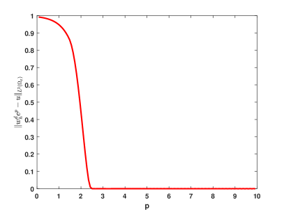
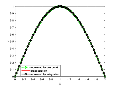
Fig. 1: Left: $\|w_{h}^{d}e^{p}-u\|_{L^{2}(\Omega_{x})}$ with respect to $p$, with $w_{h}^{d}$ computed by (4.6)-(4.7). Right: the recovery from Schrödingerization by choosing $p>p^{\Diamond}=\pi^{2}/4$.

$(\triangle p,\triangle x)$	$(\frac{10}{2^{7}},\frac{1}{2^{5}})$	order	$(\frac{10}{2^{8}},\frac{1}{2^{6}})$	order	$(\frac{10}{2^{9}},\frac{1}{2^{7}})$	order
$\|u_{h}^{d}-u\|_{L^{2}(\Omega_{x})\times L^{2}(\tilde{\Omega}_{p})}$	1.64e-03	-	3.25e-04	2.33	8.05e-05	2.01
$\|u_{d}^{*}-u\|_{L^{2}(\Omega_{x})}$	7.48e-04	-	1.86e-04	2.01	4.56e-05	2.00

Tab. 1: The convergence rates of $\|u_{h}^{d}-u\|_{L^{2}(\Omega_{x})\times L^{2}(\tilde{\Omega}_{p})}$ and $\|u_{d}^{*}-u\|_{L^{2}(\Omega_{x})}$, where $u_{h}^{d}$ is computed by (4.6)-(4.8) and $u_{d}^{*}=\frac{\int_{3}^{10}w_{h}^{d}\;\mathrm{d}p}{e^{-3}-e^{-10}}$, $\tilde{\Omega}_{p}=[3,10]$ and $\triangle t=\frac{\triangle x}{2^{3}}$.

Next, we consider another exact solution set by

$$u=\exp(-9\pi^{2}t)\sin(3\pi x),\quad\text{in}\;[0,2],$$ (6.4)

with periodic boundary conditions and the initial data is $u_{T}=\exp(-9\pi^{2})\sin(3\pi x)$. From Theorem 3.1 and Remark 3.2, we deduce that $p^{\Diamond}=\omega_{0}^{2}T=9\pi^{2}\approx 90$. From Fig. 2, it can be seen that $u=e^{p}w$ when $p\geq p^{\Diamond}\approx 90$, and the numerical solutions are very close to the real solution. In Tab. 2, the $L^{2}$ errors of the method (4.6)-(4.8) are presented. They show the optimal order $\|u_{h}^{d}-u\|_{L^{2}(\Omega_{x})\times L^{2}(\tilde{\Omega}_{p})}\sim\triangle p^{2}$, $\|u_{d}^{*}-u\|_{L^{2}(\Omega_{x})}\sim\triangle p^{2}$ are obtained when $\triangle p\to 0$, where $\tilde{\Omega}_{p}=[90,95]$, and $u_{h}^{d}=e^{p}w_{h}^{d}$, $u_{d}^{*}=\frac{\int_{90}^{95}w_{h}^{d}\;\mathrm{d}p}{e^{-90}-e^{-95}}$.

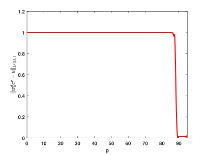
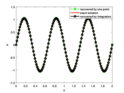
Fig. 2: Left: $\|w_{h}^{d}e^{p}-u\|_{L^{2}(\Omega_{x})}$ with respect to $p$, with $w_{h}^{d}$ computed by (4.6)-(4.7). Right: the recovery from Schrödingerization by choosing $p>p^{\Diamond}=9\pi^{2}$.

$(\triangle p,\triangle x)$	$(\frac{95}{2^{8}},\frac{1}{2^{6}})$	order	$(\frac{95}{2^{9}},\frac{1}{2^{7}})$	order	$(\frac{95}{2^{10}},\frac{1}{2^{8}})$	order
$\|u_{h}^{d}-u\|_{L^{2}(\Omega_{x})\times L^{2}(\tilde{\Omega}_{p})}$	4.73e-01	-	1.21e-01	1.96	3.07e-02	1.97
$\|u_{d}^{*}-u\|_{L^{2}(\Omega_{x})}$	1.37e-01	-	5.08e-02	1.43	1.35e-02	1.90

Tab. 2: The convergence rates of $\|u_{h}^{d}-u\|_{L^{2}(\Omega_{x})\times L^{2}(\tilde{\Omega}_{p})}$ and $\|u_{d}^{*}-u\|_{L^{2}(\Omega_{x})}$, respectively, where $u_{h}^{d}$ is computed by (4.7)-(4.8) and $u_{d}^{*}=\frac{\int_{90}^{95}w_{h}^{d}\;\mathrm{d}p}{e^{-90}-e^{-95}}$, $\tilde{\Omega}_{p}=[90,95]$, $\triangle t=\frac{\triangle x}{2^{4}}$.

6.2 Approximation of a piece-wise smooth solution

Now, we consider a piece-wise smooth solution in $(-\infty,\infty)$

$$u(x,0)=\begin{cases}-|x|+1\quad x\in[-1,1],\\ 0\quad otherwise.\end{cases}$$ (6.5)

The tests are done in the interval $x\in[-20,20]$ and $\triangle x=\frac{40}{2^{7}}$, $\triangle t=\frac{1}{2^{8}}$. We use the finite difference method to simulate the heat equation with the initial condition given by (6.5). Thus, we get the approximate solution to $u_{T}$ at $T=1$. According to Theorem 3.1, we choose $\eta_{\max}=(\frac{1}{\triangle x})^{1/2}=\sqrt{3.2}$, $(\frac{1}{\triangle x})^{1/2}=\sqrt{3.2}$ and $\frac{1}{\triangle x}=3.2$ to recover the target variables $u(t)|_{t=0.5}$, $u(t)|_{t=0.25}$ and $u(t)|_{t=0}$, respectively. Here we choose $\varepsilon=\triangle x$, $\delta(\eta_{\max})=1$ and $s=2$, $2$ and $1$, respectively. The results are shown in Fig. 3 with $u_{h}^{d}$ computed by (4.6)-(4.8) and $p\in[-30,30]$, $\triangle p=\frac{60}{2^{10}}$. From the plot of Fig. 3, we find that the error is larger when $t$ is smaller, which is consistent with the estimate in Theorem 3.1

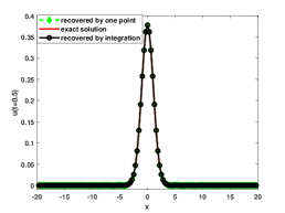
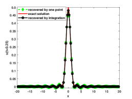
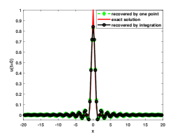
Fig. 3: The exact solution in the legend is the numerical solution at time $t=0.5$, $t=0.25$, and $t=0$, respectively, obtained by solving the forward heat conduction equation using the finite difference method. The results of Schrödingerization are shown with $\eta_{\max}=(\frac{1}{\triangle x})^{1/2}=\sqrt{3.2},(\frac{1}{\triangle x})^{1/2}=\sqrt{3.2},\frac{1}{\triangle x}=3.2$, respectively.

6.3 Input data with noises

In this test, we investigate the cases with the input data containing noises. The exact solution in $\mathbb{R}$ is set by

$$u(x,t)=\frac{1}{\sqrt{1+4t}}e^{-\frac{x^{2}}{1+4t}}.$$ (6.6)

The input data is $u_{T}^{\delta}=u_{T}+\delta_{0}\,\text{rand}(x)$. The magnitude $\delta_{0}$ indicates the noise level of the measurement data, and $\text{rand}(x)$ is a random number such that $-1\leq\text{rand}(x)\leq 1$. The tests are truncated to the interval $[-10,10]$ and $T=1$. The noise levels are $\delta_{0}=6\times 10^{-2}$, $6\times 10^{-3}$ and $6\times 10^{-4}$. We apply (4.6)-(4.8) to discretize the Schrödingerization with $p\in[-20,20]$ and $\triangle p=\frac{10}{2^{6}}$. We use the finite difference method to discretize the $x$-domain with $\triangle x=\frac{10}{2^{6}}$, $\triangle t=\frac{1}{2^{10}}$. The results are shown in Fig. 4. According to Theorem 3.2, it is hard to find $\eta_{\max}$ to satisfy $\frac{\delta(\eta_{\max})}{\eta_{\max}^{s}}+e^{\eta_{\max}^{s}T}\delta_{0}\leq\varepsilon$ for any fixed $\delta_{0}$, $T$ and $\varepsilon$. However one could choose $\eta_{\max}=\sqrt{\ln\big{(}(\frac{1}{\delta_{0}})^{\frac{1}{T}}(\ln\frac{1}{\delta_{0}})^{\frac{-s}{2T}}\big{)}}$ to get $\|u(t)-u_{\eta_{\max},\delta}(t)\|_{L^{2}(\Omega_{x})}\lesssim(\ln(\frac{1}{\delta_{0}}))^{-\frac{s}{2T}}\to 0$ as $\delta_{0}$ tends to zero under the assumption $T\leq\ln(1/\delta_{0})$, $\delta_{0}<1$. By investigating the cases of different $\delta_{0}$, we find the numerical solution of Schrödingerization approximates $u_{\eta_{\max},\delta}$ and tends to the exact solution as $\delta_{0}$ goes to zero. The oscillation of the numerical solution comes from two aspects, one is the truncation of the calculation area of $x$, and the other is the finite difference method of calculating the discontinuous input data.

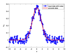
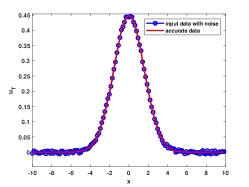
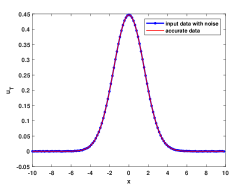
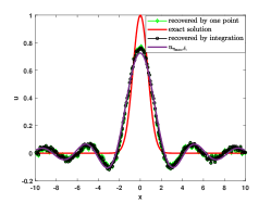
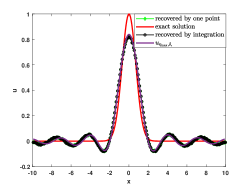
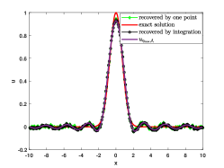
Fig. 4: The first row: input data with different noise levels from left to right. The noise levels are $6\times 10^{-2}$, $6\times 10^{-3}$ and $6\times 10^{-4}$. The second row: results of Schrödingerization computed by (4.6)-(4.8) using the input data above with $\eta_{\max}=1.5,2,2.5$,respectively.

6.4 The convection equation with imaginary wave speed

Now we consider the convection equations with imaginary wave speed to test the accuracy of the recovery. In this test, the exact solution is

$$v(t,x)=\cos(3\pi(x+t)),$$ (6.7)

and the simulation stops at $T=1$. Therefore the source term is obtained by $f=\partial_{t}u-i\partial_{x}u$ with $u$ defined in (6.7). We use the spectral method on $p$ and $x$, then get the linear system:

$$\frac{\mathrm{d}}{\mathrm{d}t}\tilde{\bm{w}}_{h}=i(D_{p}\otimes D_{x})\tilde{\bm{w}}_{h}+\tilde{\bm{f}}_{h},\quad\tilde{\bm{w}}_{h}(0)=(\Phi_{p}^{-1}\otimes\Phi^{-1}){\bm{w}}_{h}(0),$$ (6.8)

where $\tilde{\bm{f}}_{h}=(\Phi_{p}^{-1}\otimes\Phi^{-1}){\bm{f}}_{h}$, with ${\bm{f}}_{h}=\sum\limits_{j=0}^{M-1}\sum\limits_{l=0}^{N-1}f(x_{j},t)e^{-|p_{l}|}({\bm{e}}_{l}^{(N)}\otimes{\bm{e}}_{j}^{(M)})$. In order to obtain unitary dynamical systems to facilitate operation on quantum computers, one needs to use the technique of dealing with source terms in [11]. In Fig. 5, one can find $p^{\Diamond}\approx 3\pi T$ which confirms Theorem 5.1, and the numerical solutions are close to the exact one. Since the solution is not smooth enough when using the spectral method, the oscillation appears in the error between $v$ and $v_{h}^{d}$ in Fig. 5.

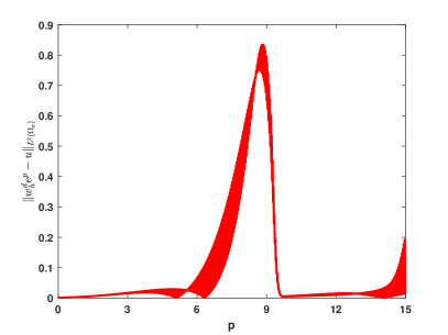
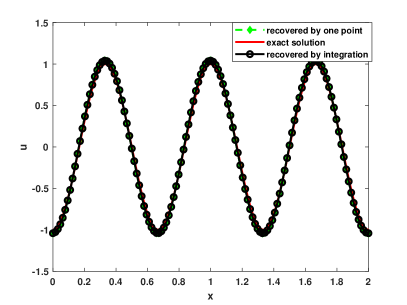
Fig. 5: Left: $\|w_{h}^{d}e^{p}-v\|_{L^{2}(\Omega_{x})}$ with respect to $p$, where $w_{h}^{d}$ is from (4.6). Right: the recovery from Schrödingerization by choosing $p>p^{\Diamond}=10$, where the numerical solution is obtained by $v_{d}^{*}=\frac{\int_{10}^{15}w_{h}^{d}\;\mathrm{d}p}{e^{-10}-e^{-15}}$, $p\in[-20,20]$, $\triangle p=\frac{10}{2^{8}}$ and $\triangle x=\frac{1}{2^{6}}$.

7 Quantum algorithms for ill-posed problems

The above numerical sche-me is a new scheme that can be used on both classical and quantum devices. The implementation scheme on quantum devices follows in much the same way as [11], since Eq. (2.1) is already of Schrödinger’s form and can be rewritten with $|w(t)\rangle=\int\bm{w}(t,p)|p\rangle dp/\|\bm{w}(t,p)\|$ obeying

$$\frac{\partial|w(t)\rangle}{\partial t}=-i(H\otimes\hat{P})|w(t)\rangle,\qquad|w_{0}\rangle=\int e^{-|p|}|p\rangle dp|u_{0}\rangle,$$ (7.1)

in the continuous-variable formalism and $\hat{P}\leftrightarrow-i\partial/\partial p$ is the momentum operator conjugate to the position operator $\hat{X}_{p}$ which has $p$ as eigenvalues and $[\hat{X}_{p},\hat{P}]=iI$. Since $H\otimes\hat{P}$ is clearly Hermitian then $|w(0)\rangle$ evolves by unitary evolution generated by the Hamiltonian $H\otimes\hat{P}$. We note that here, since we actually want to run the original PDE backwards in time, the $|u_{0}\rangle$ state above corresponds in fact to the state $|u(t=T)\rangle$. If we want the state at some $t<T$, then the time $\tau$ to run Eq. (7.1) is over $\tau\in[0,T-t]$. In the qubit formulation where $p$ is discretised, one can follow Section 4.

For the specific ill-posed problems, the difference from well-posed problems lie in the (1) cost of unitarily evolving the system in Eq. (7.1) and (2) in the cost of final measurement to retrieve $|u(t)\rangle\equiv\bm{u}(t)/\|\bm{u}(t)\|$, $t<T$, depending on the specification of possible $p^{\Diamond}$ for different problems. We note that our analysis is only valid in the case where it is possible to find $p^{\Diamond}>\eta^{2}T$, which occurs when some $\eta_{\max}<\infty$ exists. This is possible when there is either truncation in the Fourier domain of $x$ (when $\hat{u}_{T}$ has compact support) or when there is truncation in the $x$ domain directly (e.g. numerical discretisation from a finite difference scheme). These truncations or ‘regularisations’ can be achieved in both qubit-based computation and in continuous-variable based computation, but the physical origins of these truncations differ, as we will see below.

In the qubit-based formulation for instance, one can choose a finite difference scheme where $\eta_{\max}\sim O(1/\Delta x^{2})$ for the heat equation. Then the computation of the cost in evolving the system in Eq. (7.1) can be similarly derived to that already explored in the context of Schrödingerization [13]. Since it’s unitary evolution, the cost analysis is similar whether one is running forward or backward in time. The only difference is that the initial state used in the forward equation is $|u(0)\rangle$ plus the ancilla state, whereas in the backward equation it is $|u(T)\rangle$ plus the same ancilla state.

Different values of $p^{\Diamond}$ affects the probability of retrieving the correct final quantum state $|u(t)\rangle$ for $t<T$. The final step involves measurement of $p$ using for example a projective measurement $|p\rangle\langle p|$. There are in principle two schemes from Theorem 2.1, where both schemes give a success probability proportional to $K(\|\bm{u}(t)/\|\bm{u}(T)\|)^{2}$, where $K$ is a factor depending on $p^{\Diamond}_{\min}=\eta_{\max}^{2}T$, for instance see [12, 10]. The first scheme is the recovery by measurement of one point in Eq. (2.4). This corresponds to accepting the resulting state so long as the measured $p>\eta_{\max}^{2}T$. In the qubit context for example, since $\eta_{\max}\sim O(1/\Delta x^{2})$ for the heat equation, one requires enough qubits for the ancillary registers (corresponding to the $p$ dimension) which exceeds $\sim O(\log(T/\Delta x^{4}))$. In this case the largest value $K\sim e^{-2\eta^{2}_{\max}T}$. The second scheme is the recovery through integration method in Eq. (2.5). For a bounded domain, the retrieval process then involves the projection of $|w(T)\rangle$ onto the $[\eta^{2}_{\max}T,\pi L]$ domain. In this case, $K\sim(\int_{p^{\Diamond}}^{\pi L}e^{-p}dp)^{2}=(e^{-\pi L}+e^{-p^{\Diamond}})^{2}\leq(e^{-\pi L}+e^{-\eta^{2}_{\max}T})^{2}$. Thus for very large domains where $\exp(-\pi L)\sim 0$, the first and second schemes are comparable. This cost is similar for the continuous-variable and qubit-based formalisms.

It is important to point out that, if one uses the smooth initialization for the Schrödingerized equation introduced in section 4.3, and one discretises this smooth function in $p$ instead, the initial data as well as the solution in $p$ will be in $C^{k}$ for any integer $k\geq 1$. This will lead to essentially the spectral accuracy for the approximation in the extended $p$ space, if a spectral method is used. Therefore, if the desired error is $\varepsilon$, the number of mesh points used in the $p$ domain will almost be $O(\log{1/\varepsilon})$. In this case, the number of extra qubits needed due to the extra dimension, if a qubit based quantum algorithm is used, for both well-posed and ill-posed problems, becomes almost $O(\log\log{1/\varepsilon})$. This optimizes the complexity of the Schrödingerization based quantum algorithms for any dynamical system introduced in [12, 13].

In the continuous-variable formulation, how $\eta_{\max}<\infty$ arises is more subtle. The finite $\eta_{\max}$ can come instead from a kind of energy constraint $E_{\max}\sim\eta^{2}_{\max}$ on the continuous-variable ancillary quantum mode, where $\eta_{\max}$ is acting like the maximum momentum for the mode (conjugate momentum to $p$). At the measurement step, here $p^{\Diamond}_{\max}=\pi L$ is actually a maximum value of measurable $p$ by the physical measurement apparatus. The detailed analysis here is more subtle and depends on the physical system studied, so we leave this to future work.

8 Conclusions

In this paper we present computationally stable numerical methods for two ill-posed problems: the backward heat equation and the linear convection equation with imaginary wave speed. The main idea is to use Schrödingerization, which turns typical ill-posed problems into unitary dynamical systems in one higher dimension, combined with suitable truncation in the Fourier space. The Schrödingerized system is a Hamiltonian system valid both forward and backward in time, hence suitable for the design of a computationally stable numerical scheme. A key idea is given to recover the solution to the original problem from the Schrödingerized system using data from appropriate domain in the extended space. Some sharp error estimates between the approximate solution and exact solution are provided and also verified numerically. Moreover, a smooth initialization is introduced for the Schrödingerized system which leads to requiring an exponentially lower number of ancilla qubits for qubit-based quantum algorithms for any non-unitary dynamical system.

In the future this technique will be generalized to more realistic and physically interesting ill-posed problems.

References

- [1] K.A. Ames, W.C. Gordon, J.F. Epperson, and S.F. Oppenhermer. A comparison of regularizations for an ill-posed problem. Math. Comput., 67:1451–1471, 1998.
- [2] M. Bertero, P. Boccacci, and C. De Mol. Introduction to inverse problems in imaging. CRC press, 2021.
- [3] U. Biccari, Y. Song, X. Yuan, and E. Zuazua. A two-stage numerical approach for the sparse initial source identification of a diffusion–advection equation. Inverse Problems, 39(9):095003, 2023.
- [4] Heinz W. Engl, K. Kunisch, and A. Neubauer. Convergence rates for tikhonov regularisation of non-linear ill-posed problems. Inverse problems, 5(4):523, 1989.
- [5] L. C. Evans. Partial differential equations. American Mathematical Society, 2016.
- [6] T. Funada and D. Joseph. Viscous potential flow analysis of kelvin–helmholtz instability in a channel. J. Fluid Mech., 445:263–283, 2001.
- [7] D. N. Háo. A mollification method for ill-posed problems. Numerische Mathematik, 68(4):469–506, 1994.
- [8] A. Hasegawa. Plasma instabilities and nonlinear effects, volume 8. Springer Science & Business Media, 2012.
- [9] K. Höllig. Existence of infinitely many solutions for a forward backward heat equation. Trans. Amer. Math. Soc., 278(1):299–316, 1983.
- [10] S. Jin and N. Liu. Analog quantum simulation of partial differential equations. arXiv:2308.00646, 2023.
- [11] S. Jin, N. Liu, and C. Ma. On schrödingerization based quantum algorithms for linear dynamical systems with inhomogeneous terms. arXiv:2402.14696v2, 2024.
- [12] S. Jin, N. Liu, and Y. Yu. Quantum simulation of partial differential equations via schrodingerisation. arXiv preprint arXiv:2212.13969., 2022.
- [13] S. Jin, N. Liu, and Y. Yu. Quantum simulation of partial differential equations: Applications and detailed analysis. Physical Review A, 108(3):032603, 2023.
- [14] F. John. Numerical solution of the equation of heat conduction for preceding times. Ann. Mat. Pura Appl., 40:Ann. Mat. Pura Appl., 1955.
- [15] M. Jourhmane and N. S. Mera. An iterative algorithm for the backward heat conduction problem based on variable relaxation factors. Inverse Problems in Engineering, 10(4):293–308, 2002.
- [16] H. J. Kull. Theory of the rayleigh-taylor instability. Physics reports, 206(5):197–325, 1991.
- [17] R. Lattès and J. L. Lions. Méthode de quasi-réversibilité et applications. English translation: R. Bellman, Elsevier, New York, 1969.
- [18] F. Lin. Remarks on a backward parabolic problem. Methods Appl. Anal., 10(2):245–252, 2003.
- [19] K. Miller. Stabilized quasireversibility and other nearly best possible methods for non-well-posed problems. in: Symposium on Non-Well-Posed Problems and Logarithmic Convexity, in: Lecture Notes in Math., 316:161–176, 1973.
- [20] W. Miranker. A well posed problem for the backward heat equation. Proc. Amer. Math. Soc., 12:243–247, 1961.
- [21] J. Nash. Continuity of solutions of parabolic and elliptic equations. Amer. J. Math., 80(4):931–954, 1958.
- [22] R. B. Parazzoli, C.G.and Li, B. E. C. Koltenbah, and M. Tanielian. Experimental verification and simulation of negative index of refraction using snell’s law. Phys. Rev. Lett., 90(10):107401, 2003.
- [23] Z. Qian, C. L. Fu, and R. Shi. A modified method for a backward heat conduction problem. Appl. Math. Comput., 185:564–573, 2007.
- [24] R. A. Shelby, D. R. Smith, and S. Schultz. Experimental verification of a negative index of refraction. science, 292(5514):77–79, 2001.
- [25] J. Shen, T. Tang, and L. Wang. Spectral methods. Springer-Verlag Berliln Heidelberg, 2011.
- [26] R.E. Showalter. The final value problem for evolution equations. J. Math. Anal. Appl., 47:563–572, 1974.
- [27] J. Stoer, R. Bulirsch, R. Bartels, W. Gautschi, and C. Witzgall. Introduction to numerical analysis. New York: Springer-Verlag, 1980.
- [28] G. Uhlmann. Inverse problems: seeing the unseen. Bulletin of Mathematical Sciences, 4:209–279, 2014.
- [29] X. T. Xiong, C. L. Fu, and Qian Z. Two numerical methods for solving a backward heat conduction problem. Appl. Math. Comput., 179(1):370–377, 2006.