Safety-Critical Planning and Control for Dynamic Obstacle Avoidance Using Control Barrier Functions

Abstract

Dynamic obstacle avoidance is a challenging topic for optimal control and optimization-based trajectory planning problems, especially when in a tight environment. Many existing works use control barrier functions (CBFs) to enforce safety constraints within control systems. Inside these works, CBFs are usually formulated under model predictive control (MPC) framework to anticipate future states and make informed decisions, or integrated with path planning algorithms as a safety enhancement tool. However, these approaches usually require knowledge of the obstacle boundary equations or have very slow computational efficiency. In this paper, we propose a novel framework to the iterative MPC with discrete-time CBFs (DCBFs) to generate a collision-free trajectory. The DCBFs are obtained from convex polyhedra generated in sequential grid maps, without the need to know the boundary equations of obstacles. Additionally, a path planning algorithm is incorporated into this framework to ensure the global optimality of the generated trajectory. We demonstrate through numerical examples that our framework enables a unicycle robot to safely and efficiently navigate through tight and dynamically changing environments, tackling both convex and nonconvex obstacles with remarkable computing efficiency and reliability in control and trajectory generation.

I Introduction

I-A Motivation

In the robotics community, there has been considerable focus on obstacle avoidance within the realms of optimization-based control and trajectory planning. For example, formulating the task of reaching a goal while dodging obstacles and minimizing energy as a constrained optimal control problem can be achieved through the use of control barrier functions (CBFs) [1, 2]. By segmenting the timeline into brief intervals, the issue becomes a series of (potentially numerous) quadratic programs, solvable at speeds suitable for real-time operations. Nonetheless, this method might be overly aggressive because it does not incorporate forward prediction.

Model predictive control (MPC) integrated with CBFs [3] addresses safety concerns within the discrete-time domain, offering a refined control strategy by factoring in future state data over a receding horizon. However, the approach demands significant computational effort, which escalates sharply with an extended horizon, primarily due to the inherent non-linear and non-convex nature of the optimization. Another challenge with this nonlinear model predictive formulation relates to the optimization’s feasibility. Relaxation techniques introduced in reference [4] help address this, yet they apply solely to CBFs of relative-degree one, excluding those of higher order.

To overcome the challenges mentioned, in [3], we present a convex MPC framework that utilizes linearized, discrete-time CBFs (DCBFs) within an iterative approach,which is denoted as iterative MPC-DHOCBF (iMPC-DHOCBF). This method markedly decreases computational time for CBFs of high relative-degree while maintaining optimal controller performance. The feasibllity rate of iMPC-DHOCBF also outperforms the baseline method in [4] for large horizon lengths. However, linearizing DCBFs often requires knowledge of the boundary equations of obstacles, which can be challenging to ascertain in scenarios where obstacle shapes and motion patterns are complex. [5] proposed a method based on a grid map that obtains convex safety regions through a finite number of subdivisions, but it only targets for avoidance of stationary obstacles. Motivated by this, in this paper, we propose an iterative convex optimization procedure using DCBFs for dynamic obstacle avoidance in grip maps without knowing boundary equations of obstacles, which demonstrates rapid computation speed and excellent obstacle avoidance success rate.

I-B Related work

I-B1 Discrete-Time CBFs

Discrete-time CBFs (DCBFs) were introduced in [6] to facilitate safety-critical control in discrete-time systems, notably within a nonlinear MPC (NMPC) framework to form NMPC-DCBF [7], incorporating DCBF constraints over a predictive horizon. This approach extended to multi-layer control schemes in [8], considering longer horizon DCBFs for mid-level safety assurance. Variants like Generalized DCBFs (GCBFs) [9] and Discrete-Time High-Order CBFs (DHOCBFs) [10] focus on single-step constraints, enhancing feasibility but potentially compromising safety. Applications span autonomous driving [11] and legged robotics[12], with strategies ranging from first step-focused constraints [6, 9, 10] to full horizon approaches, integrating multi-layer control [8, 11] or planning [12] for platform-specific optimization. The related work mentioned above obtains DCBFs through analytical geometry, thus requiring knowledge of the obstacle boundary equations. In this paper, we generate convex polyhedra in the grid map, without the need to know the boundary equations of obstacles. We use the interiors of these polyhedra to represent safe areas, while their boundaries are transformed into linear DHOCBFs as safety constraints.

I-B2 Model Predictive Control (MPC)

MPC is a key technique in control systems for designing robot controllers in robotic manipulation and locomotion [13, 14], offering optimization-based control strategies. Stability in these systems is achieved by integrating discrete-time control Lyapunov functions (DCLFs) within MPC frameworks for efficient real-time control, even with limited computational power. Recent research like [15] increasingly focuses on safety in robotics, a crucial aspect for practical applications. Some studies introduce repelling functions [1, 16] to address safety, while others [17, 18, 19] specifically tackle obstacle avoidance as a safety measure. Typically, these safety considerations are incorporated as constraints within optimization problems. This paper can be seen in the context of MPC with safety constraints.

I-B3 Path Planning Algorithms

In motion planning, a variety of methods can be employed to secure effective collision-free paths. Sampling-based algorithms, such as Rapidly-Exploring Random Trees (RRT) and Probabilistic Roadmaps (PRM), achieve impressive results in high-dimensional complex spaces by randomly expanding searches within the feasible space to find a feasible path, although their probabilistic completeness does not guarantee the prompt identification of the optimal feasible solution.

Conversely, grid search-based algorithms (like Dijkstra, A*, and their variants) offer resolution completeness ensuring the determination of the shortest path between nodes in grid-based searches. A*, an extension of the Dijkstra algorithm, utilizes a heuristic approach to estimate the overall path cost, thereby outperforming the Dijkstra algorithm. Jump Point Search (JPS) [20], the optimized algorithm of A*, was proposed for uniform grids to accelerate search speeds by eliminating certain nodes in the grid based on the setup of jump points. It represents a method of graph pruning that reduces symmetry in searches with minimal computational cost, making it suitable for large-scale searches in large, uniform open spaces. In this paper, we use the optimal path produced by JPS as reference trajectory that makes the control problem fast.

I-C Contributions

We propose a novel framework to the iterative MPC with DHOCBFs that can generate a collision-free trajectory and computes fast. In particular, the contributions are as follows:

• We present a model predictive control strategy for safety-critical tasks, where the safety-critical constraints can be enforced by DHOCBFs. The DHOCBF constraints are obtained from convex polyhedra generated in sequential grid maps, without the need to know the boundary equations of obstacles.

• We propose a novel optimal control framework for guaranteeing safety in a dynamic environment, where the dynamic environment consists of grid maps that change over time. A rapid path planning algorithm is incorporated into the control framework to generate optimal trajectory in each grid map. DHOCBFs and system dynamics serve as linear constraints to make control problem a convex optimization. Our framework synthesize the convex optimization and sequential grid maps with rapid computational speed.

• We show through numerical examples that the proposed framework enables a unicycle robot to navigate with safe maneuvers through tight and dynamic environments with convex or nonconvex shape obstacles using rapid control and trajectory generation.

II Preliminaries

In this section, we introduce some definitions and results on DHOCBF and JPS.

II-A subsec: Discrete-Time High-Order Control Barrier Function (DHOCBF)

In this paper, we consider a discrete-time control system in the form

$$\mathbf{x}_{t+1}=f(\mathbf{x}_{t},\mathbf{u}_{t}),$$ (1)

where $\mathbf{x}_{t}\in\mathcal{X}\subset\mathbb{R}^{n}$ represents its state at discrete time $t\in\mathbb{N},\mathbf{u}_{t}\in\mathcal{U}\subset\mathbb{R}^{q}$ is the control input, and $f:\mathbb{R}^{n}\rightarrow\mathbb{R}^{q}$ is a locally Lipschitz function capturing the dynamics of the system. We interpret safety forward invariance of a set $\mathcal{C}$. A system is considered safe if, once it starts within set $\mathcal{C}$, it remains in $\mathcal{C}$ for all future times. We consider the set $\mathcal{C}$ as the super-level set of a function $h:\mathbb{R}^{n}\to\mathbb{R}$:

$$\mathcal{C}\coloneqq\{\mathbf{x}\in\mathbb{R}^{n}:h(\mathbf{x})\geq 0\}.$$ (2)

Definition 1 (Relative degree [21]).

The output $\mathbf{y}=h(\mathbf{x})$ of system (1) is said to have relative degree $m$ with respect to dynamics (1) if $\forall t\in\mathbb{N},$

$$\begin{split}\mathbf{y}_{t+i}=h(\bar{f}_{i-1}(f(\mathbf{x}_{t},\mathbf{u}_{t}))),\ i\in\{1,2,\dots,m\},\\ \text{s.t.}\ \frac{\partial\mathbf{y}_{t+m}}{\partial\mathbf{u}_{t}}\neq 0_{q},\frac{\partial\mathbf{y}_{t+i}}{\partial\mathbf{u}_{t}}=0_{q},\ i\in\{1,2,\dots,m-1\}.\end{split}$$ (3)

Informally, the relative degree $m$ is the number of steps (delay) in the output $\mathbf{y}_{t}$ in order for the control input $\mathbf{u}_{t}$ to appear. In the above definition, we use $\bar{f}(\mathbf{x})$ to denote the uncontrolled state dynamics $f(\mathbf{x},0)$. The subscript $i$ of function $\bar{f}(\cdot)$ denotes the $i$-times recursive compositions of $\bar{f}(\cdot)$, i.e., $\bar{f}_{i}(\mathbf{x})=\underset{i\text{-times}~{}~{}~{}~{}~{}~{}~{}~{}~{}~{}~{}~{}~{}}{\underbrace{\bar{f}(\bar{f}(\dots,\bar{f}}(\bar{f}_{0}(\mathbf{x}))))}$ with $\bar{f}_{0}(\mathbf{x})=\mathbf{x}$.

We assume that $h(\mathbf{x}_{t})$ has relative degree $m$ with respect to system (1) based on Def. 1. Starting with $\psi_{0}(\mathbf{x}_{t})\coloneqq h(\mathbf{x}_{t})$, we define a sequence of discrete-time functions $\psi_{i}:\mathbb{R}^{n}\to\mathbb{R}$, $i=1,\dots,m$ as:

$$\psi_{i}(\mathbf{x}_{t})\coloneqq\bigtriangleup\psi_{i-1}(\mathbf{x}_{t},\mathbf{u}_{t})+\alpha_{i}(\psi_{i-1}(\mathbf{x}_{t})),$$ (4)

where $\bigtriangleup\psi_{i-1}(\mathbf{x}_{t},\mathbf{u}_{t})\coloneqq\psi_{i-1}(\mathbf{x}_{t+1})-\psi_{i-1}(\mathbf{x}_{t})$, and $\alpha_{i}(\cdot)$ denotes the $i^{th}$ class $\kappa$ function which satisfies $\alpha_{i}(\psi_{i-1}(\mathbf{x}_{t}))\leq\psi_{i-1}(\mathbf{x}_{t})$ for $i=1,\ldots,m$. A sequence of sets $\mathcal{C}_{i}$ is defined based on (4) as

$$\mathcal{C}_{i}\coloneqq\{\mathbf{x}\in\mathbb{R}^{n}:\psi_{i}(\mathbf{x})\geq 0\},\ i=\{0,\ldots,m-1\}.$$ (5)

Definition 2 (DHOCBF [10]).

Let $\psi_{i}(\mathbf{x}),\ i\in\{1,\dots,m\}$ be defined by (4) and $\mathcal{C}_{i},\ i\in\{0,\dots,m-1\}$ be defined by (5). A function $h:\mathbb{R}^{n}\to\mathbb{R}$ is a Discrete-Time High-Order Control Barrier Function (DHOCBF) with relative degree $m$ for system (1) if there exist $\psi_{m}(\mathbf{x})$ and $\mathcal{C}_{i}$ such that

$$\psi_{m}(\mathbf{x})\geq 0,\ \forall\mathbf{x}_{t}\in\mathcal{C}_{0}\cap\dots\cap\mathcal{C}_{m-1},\forall t\in\mathbb{N}.$$ (6)

Theorem 1 (Safety Guarantee [10]).

Given a DHOCBF $h(\mathbf{x})$ from Def. 2 with corresponding sets $\mathcal{C}_{0},\dots,\mathcal{C}_{m-1}$ defined by (5), if $\mathbf{x}_{0}\in\mathcal{C}_{0}\cap\dots\cap\mathcal{C}_{m-1},$ then any Lipschitz controller $\mathbf{u}$ that satisfies the constraint in (6), $\forall t\geq 0$ renders $\mathcal{C}_{0}\cap\dots\cap\mathcal{C}_{m-1}$ forward invariant for system (1), $i.e.,\mathbf{x}_{t}\in\mathcal{C}_{0}\cap\dots\cap\mathcal{C}_{m-1},\forall t\geq 0.$

The function $\psi_{i}(\mathbf{x})$ in (4) is called a $i^{th}$ order discrete-time control barrier function (DCBF). Since satisfying the $i^{th}$ order DCBF constraint ($\psi_{i}(\mathbf{x})\geq 0$) is a sufficient condition for rendering $\mathcal{C}_{0}\cap\dots\cap\mathcal{C}_{i-1}$ forward invariant for system (1) as shown above, it is not necessary to formulate DCBF constraints up to $m^{th}$ order as (6) if the control input $\mathbf{u}_{t}$ could be involved in some optimal control problem. In other words, the highest order for DCBF could be $m_{\text{cbf}}$ with $m_{\text{cbf}}\leq m.$ In this paper, one simple method to define a $i^{th}$ order DCBF $\psi_{i}(\mathbf{x})$ in (4) is

$$\psi_{i}(\mathbf{x}_{t})\coloneqq\bigtriangleup\psi_{i-1}(\mathbf{x}_{t},\mathbf{u}_{t})+\gamma_{i}\psi_{i-1}(\mathbf{x}_{t}),$$ (7)

where $0<\gamma_{i}\leq 1,i\in\{1,\dots,m_{\text{cbf}}\}$.

The expression in (7) follows the format of the first order DCBF proposed in [6] and could be used to define a DHOCBF with arbitrary relative degree.

II-B Jump Point Search

A graph search (path planning) algorithm can then be used to identify a valid path that avoids collisions within the grids occupied by obstacles. As we discussed in Sec. I-B3, JPS is suitable for rapid path planning. we define a path, denoted as $\pi=\left\langle n_{i},\ldots,n_{j}\right\rangle$, as a sequence of nodes or states extending from node $i$ to node $j$. The length (or cost) of this path is represented by $\text{len}(\pi)$. We introduce the notation $x$ to refer to a specific node, $p(x)$ to denote the parent node of $x$, and $\text{neighbors}(x)$ to describe the set of nodes adjacent to $x$. Additionally, the node $n$ is defined as an element within the set of $\text{neighbors}(x)$. The expression $\pi\backslash x$ signifies that node $x$ is omitted from the path.

In a 2-D map, each node may have up to 8 neighbors. The cost incurred when moving straightly (horizontally or vertically) to a traversable neighbor (not occupied by obstacles) is 1, while moving diagonally has a cost of $\sqrt{2}$. For straight moves, if node $n$ can be reached from $x$’s parent $p(x)$ with the less or equal cost without passing through $x$, i.e., $len(\left\langle p(x),\dots,n\right\rangle\backslash x)\leq len(\left\langle p(x),x,n\right\rangle)$, JPS will prune this neighbor $n$ from exploration. In diagonal moves, the path excluding $x$ must be strictly shorter, $len(\left\langle p(x),\dots,n\right\rangle\backslash x)<len(\left\langle p(x),x,n\right\rangle)$, leading to the pruning of node $n$. The natural neighbors of $x$ are those that remain after pruning, assuming $\text{neighbors}(x)$ does not include obstacles. Force neighbors refer to specific neighboring nodes that may not lie directly on the current path but must be examined to ensure the identification of the shortest path, which must satisfy two conditions. 1) $n$ is not a natural neighbour 2) $len(\left\langle p(x),x,n\right\rangle)<len(\left\langle p(x),\dots,n\right\rangle\backslash x)$. A node qualifies as a jump point if it meets one of the following criteria: it is either the initial or terminal node, it has a forced neighbor, or, in the case of diagonal movement, it leads directly to another jump point, as detailed in [20] and [5].

Starting from initial node, the algorithm recursively searches for new jump points in every direction until the terminal node is found or a dead end is reached in that direction. Upon reaching the terminal node, it backtracks through the jump points to construct the shortest path, $\pi=\left\langle n_{0},n_{1},\dots,n_{E}\right\rangle$, from start to finish. Path searching with jump point pruning has been proven to be cost-optimal in [20].

III Methodology

The comprehensive structure of our algorithm is depicted in Alg. 1, which integrates iterative MPC with pathfinding algorithms and DHOCBF under linear safety constraints. The iterative MPC cannot perfectly help robot adhere to the optimal path we have identified, and the optimal path may not necessarily be dynamically feasible, so even though the optimal path is safe, there is still a possibility of colliding with obstacles during the path-following process. Therefore, we utilize DHOCBF to ensure safety throughout the path-following phase. Since the iterative MPC looks ahead into the future over a specified prediction horizon, we assume the future information about dynamic obstacles in grid maps up to the horizon is known to us.

Algorithm 1 iMPC-DHOCBF [3] for Sequential Grid Maps

0:  System dynamics (1), initial state $\mathbf{x}(0)$, ending location $n_{E}$, sequential grid maps of obstacles $[G_{0},G_{1},\dots,G_{t_{\text{sim}+N}}].$

0:  Safety-critical optimal control for path following and dynamic obstacle avoidance.

1:  Set initial guess $\bar{\mathbf{U}}_{0}^{0}=0$ at $t=0$.

2:  Propagate with system dynamics to get initial guess of states $\bar{\mathbf{X}}_{0}^{0}$ from initial state $\mathbf{x}(0)$.

3:  for $t\leq t_{\text{sim}}-1$ do

4:     Initialize $j=0$.

5:     Get sequential grid maps from $G_{t}$ to $G_{t+N}.$

6:     Extract current location $n_{t}$ from $\mathbf{x}(t),$ use path planning algorithm to find the optimal path $\pi_{t}=\left\langle n_{t},\dots,n_{E}\right\rangle.$

7:     Reconstruct the path to get $[\mathbf{x}_{r,t},\mathbf{x}_{r,t+1},\dots,\mathbf{x}_{r,t+N}],$ which is the reference state matrix used in the cost $J$.

8:     while  Iteration $j$ (not converged OR $j<j_{\text{max}}$) do

9:        Linearize system dynamics with $\bar{\mathbf{X}}_{t}^{j},\bar{\mathbf{U}}_{t}^{j}$ (constraints).

10:        Get linear DHOCBFs $h_{\text{scp}}(\mathbf{x}_{t,k}^{j}|\bar{\mathbf{x}}_{t,k}^{j}),k\in\left\{1,\dots,N\right\}$ from safe convex polyhedra.

11:        Solve a convex finite-time constrained optimal control problem (CFTOC) with cost $J$ and linear constraints to get optimal values of states and inputs $\mathbf{X}_{t}^{*,j}$, $\mathbf{U}_{t}^{*,j}$.

12:        $\bar{\mathbf{X}}_{t}^{j+1}=\mathbf{X}_{t}^{*,j},\bar{\mathbf{U}}_{t}^{j+1}=\mathbf{U}_{t}^{*,j}$, $j=j+1$

13:     end while

14:     Extract optimized states and inputs $\mathbf{X}_{t}^{*}=\mathbf{X}_{t}^{*,j},\mathbf{U}_{t}^{*}=\mathbf{U}_{t}^{*,j}$ from last iteration and extract $\mathbf{u}_{t,0}^{*}$ from $\mathbf{U}_{t}^{*}$.

15:     Apply $\mathbf{u}_{t,0}^{*}$ with respect to system dynamics (1) to get $\mathbf{x}_{t+1}=f(\mathbf{x}_{t},\mathbf{u}_{t,0}^{*})$, and record $\mathbf{x}(t+1)=\mathbf{x}_{t+1}$.

16:     Update $\bar{\mathbf{U}}_{t+1}^{0}$ with $\mathbf{U}_{t}^{*}$ and propagate to calculate $\bar{\mathbf{X}}_{t+1}^{0}$.

17:     $t=t+1$.

18:  end for

19:  return  closed-loop trajectory $[\mathbf{x}(0),\dots,\mathbf{x}(t_{\text{sim}})]$

The algorithm described in Alg. 1 contains an iterative optimization at each time step $t$, which is denoted as iMPC-DHOCBF [3]. In each iteration $j$ of our optimization problem, we address three distinct components: (1) solve a convex finite-time optimal control (CFTOC) problem with linearized dynamics and linear DHOCBFs $h_{\text{scp}}(\bar{\mathbf{x}}_{t,k}^{j}),k\in\left\{1,\dots,N\right\}$, (2) check convergence criteria, (3) update state and input vectors for next iteration. Notice that the open-loop trajectory with updated states $\bar{\mathbf{X}}_{t}^{j}=[\bar{\mathbf{x}}_{t,0}^{j},\dots,\bar{\mathbf{x}}_{t,N-1}^{j}]$ and inputs $\bar{\mathbf{U}}_{t}^{j}=[\bar{\mathbf{u}}_{t,0}^{j},\dots,\bar{\mathbf{u}}_{t,N-1}^{j}]$ is passed between iterations, which allows iterative linearization for system dynamics locally. The DHOCBFs $h_{\text{scp}}(\bar{\mathbf{x}}_{t,k}^{j})$ can be extended to higher order DCBFs, which work as safety constraints in CFTOC problem. As discussed in Sec. II-A and (7), “higher order” implies that the relative degree of DCBFs is $m_{\text{cbf}}$ with $1\leq m_{\text{cbf}}\leq m$.

The iteration concludes once the convergence error function $e(\mathbf{X}_{t}^{*,j},\mathbf{U}_{t}^{*,j},\bar{\mathbf{X}}_{t}^{j},\bar{\mathbf{U}}_{t}^{j})$ falls within a predefined normalized convergence criterion, with $\mathbf{X}_{t}^{*,j}=[\mathbf{x}_{t,0}^{*,j},\dots,\mathbf{x}_{t,N}^{*,j}]$, $\mathbf{U}_{t}^{*,j}=[\mathbf{u}_{t,0}^{*,j},\dots,\mathbf{u}_{t,N-1}^{*,j}]$ denoting the optimized states and inputs, respectively at iteration $j.$ To cap the iteration count, we enforce $j\leq j_{\text{max}}$, where $j_{\text{max}}$ represents the maximum allowable number of iterations. Thus, the iterative optimization process halts upon reaching a local optimal minimum for the cost function, meeting the convergence criterion, or when the iteration count equals $j_{\text{max}}$. The optimized states $\mathbf{X}_{t}^{*}$ and inputs $\mathbf{U}_{t}^{*}$ are passed to the iMPC-DHOCBF formulation for the next time instant. At each step, we log the updated state as it evolves according to the system dynamics over a specified discretization interval. This process enables us to derive the output closed-loop trajectory using iMPC-DHOCBF approach.

III-A Dynamic Path Planning-Dynamic JPS

In Alg. 1, we can use JPS to find the optimal path. Since the locations of dynamic obstacles in grid maps vary over time, we need to replan the path to the destination after each movement of the robot and this explains the necessity of dynamic path planning. At each time step $t$, the system state $\mathbf{x}(t)$ is updated by solving the CFTOC and the corresponding location $n_{t}$ can be extracted from $\mathbf{x}(t).$ The safe and shortest path $\pi_{t}=\left\langle n_{t},n_{1},\dots,n_{E}\right\rangle,$ which consists of a series of point coordinates from $n_{t}$ to $n_{E}$, can be repeatedly found by repeatedly calling JPS, and thus each path consists of straight line segments of varying lengths. By following these paths, our robot also walks a relatively short path under the action of the safety-critical controller.

III-B Path Reconstruction

To illustrate the necessity of path reconstruction, consider a simplified unicycle model in the form

$$\begin{bmatrix}x_{t+1}{-}x_{t}\\ y_{t+1}{-}y_{t}\\ \theta_{t+1}{-}\theta_{t}\end{bmatrix}{=}\begin{bmatrix}v\cos(\theta_{t})\Delta t\\ v\sin(\theta_{t})\Delta t\\ 0\end{bmatrix}{+}\begin{bmatrix}0\\ 0\\ \Delta t\end{bmatrix}u_{t},$$ (8)

where $\mathbf{x}_{t}=[x_{t},y_{t},\theta_{t}]^{T}$ captures the 2-D location and heading angle, $v$ denotes constant linear speed, and $\mathbf{u}_{t}$ represents angular velocity. $\Delta t$ denotes the discretized time interval. Note that the optimal path we get in Sec. III-A only contains information about desired 2-D locations, i.e., the desired heading angles are lost. Moreover, the distance between points on the optimal path $\pi_{t}$ may be too large to follow. These reasons all lead to the optimal path $\pi_{t}$ not being viable as reference state vectors in cost $J.$ To address this problem, we propose the path transformation approach next.

Given a constant speed $v$ in the simplified unicycle model, the step size of robot is $L=v*\Delta t.$ The maximum number of steps between points $n_{t}$ and $n_{1}$ is $i_{1}=\frac{S_{1}-(S_{1}\bmod L)}{L},$ where $S_{1}=\sqrt{(n_{1}-n_{t})^{T}(n_{1}-n_{t})}.$ A list of reference state vectors up to $i_{1}$ are then expressed as

$$\underbrace{\begin{bmatrix}x_{r,t+i+1}\\ y_{r,t+i+1}\\ \theta_{r,t+i+1}\end{bmatrix}}_{\mathbf{x}_{r,t+i+1}}=\begin{bmatrix}x_{r,t+i}+v\cos{(\theta_{r,t+i})}\\ y_{r,t+i}+v\sin{(\theta_{r,t+i})}\\ atan2(\frac{n_{1}[2]-n_{t}[2]}{n_{1}[1]-n_{t}[1]})\end{bmatrix},$$ (9)

where $i\in\{0,1,\dots,i_{1}-1\},$ and $\mathbf{x}_{r,t}=\begin{bmatrix}x_{r,t}\\ y_{r,t}\\ \theta_{r,t}\end{bmatrix}=\begin{bmatrix}n_{t}[1]\\ n_{t}[2]\\ \theta_{r,t+1}\end{bmatrix}.$ Replace $n_{t},n_{1}$ with $\begin{bmatrix}x_{r,t+i_{1}}\\ y_{r,t+i_{1}}\end{bmatrix},n_{2}$ respectively. Similarly we have $i_{2}=\frac{S_{2}-(S_{2}\bmod L)}{L},$ where $S_{2}=\sqrt{(n_{2}-n_{t+i_{1}})^{T}(n_{2}-n_{t+i_{1}})}.$ We can obtain a list of reference state vectors up to $i_{2}$ based on (9) then replace $n_{t+i_{1}},n_{2}$ with $\begin{bmatrix}x_{r,t+i_{2}}\\ y_{r,t+i_{2}}\end{bmatrix},n_{3}$ respectively. Do the above process repeatedly until we find a number $i_{m}(m\geq 1)$ which satisfies the inequality $\sum_{j=1}^{m}i_{j}\geq N.$ We can stack the past reference state vectors into a reference state matrix as $[\mathbf{x}_{r,t},\mathbf{x}_{r,t+1},\dots,\mathbf{x}_{r,t+N}].$ The connection of each point (denoted by the first two rows of reference state matrix) depicts the reconstructed path, which is slightly different from the optimal path $\pi_{t}.$ As $\Delta t$ decreases, this difference will also gradually diminish to a negligible extent. The transformation approach we propose here targets a special class of systems with well-defined kinematics-geometric structures (e.g., a simplified unicycle model in (8)). This approach can be extended to other types of systems, as long as we can find a reasonable transformation to get the reference state matrix $[\mathbf{x}_{r,t},\mathbf{x}_{r,t+1},\dots,\mathbf{x}_{r,t+N}].$

Another approach that might be suitable for all dynamic systems purely depends on parameters tuning. We can just insert $N$ points on the path $\pi_{t}$ as reference locations (e.g., $[x_{r,t},x_{r,t+1},\dots,x_{r,t+N}],[y_{r,t},y_{r,t+1},\dots,y_{r,t+N}]$) and predefine other reference states except locations (e.g., $[\theta_{r,t},\theta_{r,t+1},\dots,\theta_{r,t+N}]$), then formulate them into a cost function as

$$J=\sum_{k=0}^{N-1}(||\mathbf{x}_{t,k}^{j}-\mathbf{x}_{r,t+k}||_{Q}^{2}+||\mathbf{x}_{t,N}^{j}-\mathbf{x}_{r,t+N}||_{P}^{2}),$$ (10)

where $\mathbf{x}_{r,t+k}=[x_{r,t+k},y_{r,t+k},\theta_{r,t+k}]^{T},k\in\left\{0,\dots,N\right\}$ denotes the reference state vector at each time step. $Q,P$ are diagonal matrices served as weight matrices. We can increase the weights in the weight matrices corresponding to reference locations (e.g., the first and second elements on diagonal in $Q,P$) to focus more on minimizing the deviation from the desired path.

III-C Linearization of Dynamics

At iteration $j$, an improved vector $\mathbf{u}_{t,k}^{j}$ is achieved by linearizing the system around $\bar{\mathbf{x}}_{t,k}^{j},\bar{\mathbf{u}}_{t,k}^{j}$:

$$\begin{split}\mathbf{x}_{t,k+1}^{j}{-}\bar{\mathbf{x}}_{t,k+1}^{j}{=}A^{j}(\mathbf{x}_{t,k}^{j}{-}\bar{\mathbf{x}}_{t,k}^{j})+B^{j}(\mathbf{u}_{t,k}^{j}{-}\bar{\mathbf{u}}_{t,k}^{j}),\end{split}$$ (11)

where $0\leq j<j_{\text{max}}$; $k$ and $j$ represent open-loop time step and iteration indices, respectively. We also have

$$A^{j}=D_{\mathbf{x}}f(\bar{\mathbf{x}}_{t,k}^{j},\bar{\mathbf{u}}_{t,k}^{j}),\ B^{j}=D_{\mathbf{u}}f(\bar{\mathbf{x}}_{t,k}^{j},\bar{\mathbf{u}}_{t,k}^{j}),$$ (12)

where $D_{\mathbf{x}}$ and $D_{\mathbf{u}}$ denote the Jacobian of the system dynamics $f(\mathbf{x},\mathbf{u})$ with respect to the state $\mathbf{x}$ and the input $\mathbf{u}$. This approach allows to linearize the system at $(\bar{\mathbf{x}}_{t,k}^{j},\bar{\mathbf{u}}_{t,k}^{j})$ locally between iterations. The convex system dynamics constraints are detailed in (11), given that all nominal vectors $(\bar{\mathbf{x}}_{t,k}^{j},\bar{\mathbf{u}}_{t,k}^{j})$ from the current iteration are constant, having been constructed from the previous iteration $j-1$.

III-D DHOCBF-Safe Convex Polyhedron

In this section, we show how to get linear DCBFs up to the highest order from Safe Convex Polyhedron (SCP). Note that in a 2-D map it is in fact a convex polygon. Based on the grid map $G_{t+k}$, at iteration $j$, in order to formulate DHOCBF candidates $h_{\text{scp}}(\mathbf{x}_{t,k}^{j}|\bar{\mathbf{x}}_{t,k}^{j})$, a square (depicted by blue square with dashed lines in Fig. 1) delineating the obstacle detection range is drawn, with its geometric center being the current position of the robot ($\bar{\mathbf{x}}_{t,k}^{j}$). We segment the boundaries of obstacles within the square, identifying a series of points (depicted by black points), then we find the point closest to the robot among these points and draw a perpendicular line segment through this point to the line connecting the point and the robot. This line segment belongs to the boundary of SCP (depicted by a red line segment), which designates the area on the side opposite the robot as the detected zone and excludes it (depicted by grey). Repeat the above process for undetected area within the square until the closed boundary of SCP is found. This boundary consists of $n_{\text{scp}}$ line segments. Some of them are expressed by linear equations $h_{l}(\mathbf{x}_{t,k}^{j}|\bar{\mathbf{x}}_{t,k}^{j})=a_{l}x_{t,k}^{j}+b_{l}y_{t,k}^{j}+c_{l},l\in\left\{1,\dots,l_{\text{scp}}\right\},l_{\text{scp}}\leq n_{\text{scp}}.$ The parameters are obtained by

$$\begin{split}&a_{l}=\bar{x}_{t,k}^{j}-\tilde{x}_{t,k}^{j,l},\\ &b_{l}=\bar{y}_{t,k}^{j}-\tilde{y}_{t,k}^{j,l},\\ &c_{l}=-(\bar{x}_{t,k}^{j}-\tilde{x}_{t,k}^{j,l})\tilde{x}_{t,k}^{j,l}-(\bar{y}_{t,k}^{j}-\tilde{y}_{t,k}^{j,l})\tilde{y}_{t,k}^{j,l},\end{split}$$ (13)

where $(\tilde{x}_{t,k}^{j,l},\tilde{y}_{t,k}^{j,l})$ denotes the $l^{th}$ closest point on $l^{th}$ line segment. Other segments are from four sides of the square. This allows us to define a safe region (inner area of the polygon) expressed by ${C}_{t,i}^{j}\coloneqq\{\mathbf{x}_{t,i}^{j}\in\mathbb{R}^{n}:h_{\text{scp}}(\mathbf{x}_{t,k}^{j}|\bar{\mathbf{x}}_{t,k}^{j})\geq 0\},h_{\text{scp}}(\mathbf{x}_{t,k}^{j}|\bar{\mathbf{x}}_{t,k}^{j})\geq 0\Longleftrightarrow\left\{h_{1}(\mathbf{x}_{t,k}^{j}|\bar{\mathbf{x}}_{t,k}^{j})\geq 0,\dots,h_{n_{\text{scp}}}(\mathbf{x}_{t,k}^{j}|\bar{\mathbf{x}}_{t,k}^{j})\geq 0\right\}.$ The relative degree of $h_{\text{scp}}(\mathbf{x}_{t,k}^{j}|\bar{\mathbf{x}}_{t,k}^{j})$ with respect to system (1) is $m.$

In order to guarantee safety with forward invariance based on Thm. 1, two sufficient conditions need to be satisfied: (1) the sequence of DHOCBFs $\tilde{\psi}_{0}^{n}(\cdot),\dots,\tilde{\psi}_{m_{\text{cbf}}-1}^{n}(\cdot)$ is larger or equal to zero at the initial condition $\mathbf{x}_{t}$, and (2) the highest-order DCBF constraint $\tilde{\psi}_{m_{\text{cbf}}}^{n}(\mathbf{x})\geq 0$ is always satisfied, where $\tilde{\psi}_{i}^{n}(\cdot)$ is defined as:

$$\begin{split}\tilde{\psi}_{0}^{n}(\mathbf{x}_{t,k}^{j})\coloneqq&h_{n}(\mathbf{x}_{t,k}^{j}|\bar{\mathbf{x}}_{t,k}^{j})\\ \tilde{\psi}_{i}^{n}(\mathbf{x}_{t,k}^{j})\coloneqq&\tilde{\psi}_{i-1}^{n}(\mathbf{x}_{t,k+1}^{j})-\tilde{\psi}_{i-1}^{n}(\mathbf{x}_{t,k}^{j}){+}\gamma_{i}^{n}\tilde{\psi}_{i-1}^{n}(\mathbf{x}_{t,k}^{j}).\end{split}$$ (14)

Here, we have $0<\gamma_{i}^{n}\leq 1$, $i\in\{1,\dots,m_{\text{cbf}}\},n\in\{1,\dots,n_{\text{scp}}\},$ and $m_{\text{cbf}}\leq m$ (as in (7)).

Note that $n_{\text{scp}}$ is not predefined. As the number of obstacles within the square increases, $n_{\text{scp}}$ may become very large. The swift rise in the number of constraints may make solving the optimization problem infeasible. In order to handle this issue, we introduce a slack variable $\omega_{t,k,i}^{j,n}$ with a corresponding decay rate $(1-\gamma_{i}^{n}).$ Similar to [3], we reformulate $\tilde{\psi}_{i}^{n}(\mathbf{x}_{t,k}^{j})\geq 0$ in (14) as

$$\begin{split}&\tilde{\psi}_{i-1}^{n}(\mathbf{x}_{t,k}^{j})+\sum_{\nu=1}^{i}Z_{\nu,i}^{n}(1-\gamma_{i}^{n})^{k}\tilde{\psi}_{0}^{n}(\mathbf{x}_{t,\nu}^{j})\geq\\ &\quad\omega_{t,k,i}^{j,n}Z_{0,i}^{n}(1-\gamma_{i}^{n})^{k}\tilde{\psi}_{0}^{n}(\mathbf{x}_{t,0}^{j}),j\leq j_{\text{max}}\in\mathbb{N}^{+},\\ &n\in\{1,\dots,n_{\text{scp}}\},\ i\in\{1,\dots,m_{\text{cbf}}\},\ \omega_{t,k,i}^{j,n}\in\mathbb{R}.\end{split}$$ (15)

In the above, the slack variable $\omega_{t,k,i}^{j,n}$ is a decision variable, determined by minimizing a term in the cost function to meet the DCBF constraints from the initial condition at any given time step (see [3]). $Z_{\nu,i}$ is a constant that aims to make constraint (15) linear in terms of decision variables $\mathbf{x}_{t,k}^{j},\omega_{t,k,i}^{j,n},$ and can be obtained as follows. When $2\leq i,\nu\leq i-2$, we have

$$\begin{split}Z_{\nu,i}^{n}=\sum_{l=1}^{l_{\text{max}}}[(\gamma_{\zeta_{1}}-1)(\gamma_{\zeta_{2}}-1)\cdots(\gamma_{\zeta_{i-\nu-1}}-1)]_{l},\\ \zeta_{1}<\zeta_{2}<\dots<\zeta_{i-\nu-1},\zeta_{s}\in\{1,2,\dots,i-1\},\end{split}$$ (16)

where $[\cdot]_{l}$ denotes the $l^{th}$ combination of the product of the elements in parenthesis, therefore we have $l_{\text{max}}=\binom{i-1}{i-\nu-1}$. $\zeta_{s}$ denote all $\zeta$ in (16). For the case $\nu=i-1$, if $2\leq i$, we define $Z_{\nu,i}^{n}=-1$; if $i=1$, we define $Z_{\nu,i}^{n}=1$. Beside that, we define $Z_{\nu,i}^{n}=0$ for the case $\nu=i$.

Remark 1.

Note that in Sec. III-D, we illustrate the process of getting the safe convex polygon in a 2-D map. We can mimic the process to get a safe convex polyhedron in a 3-D map, i.e., draw a normal plane section (face of polyhedron) through the closest point to the line connecting the point and the robot to get candidate DHOCBF $h_{n}(\mathbf{x}_{t,k}^{j}|\bar{\mathbf{x}}_{t,k}^{j})$, which can be extended into DCBFs (14) as safety constraints. A similar method, named Safe Flight Corridor (SFC) to get safe convex polyhedron for a non-point robot based on a shrinking ellipsoid was investigated in [5].

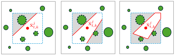
Figure 1: A schematic diagram illustrating how to find the SCP (red). The obstacle detection range is denoted by blue dashed square with geometry center $\bar{\mathbf{x}}_{t,k}^{j}$. The obstacles are depicted by green circles.

III-E CFTOC Problem

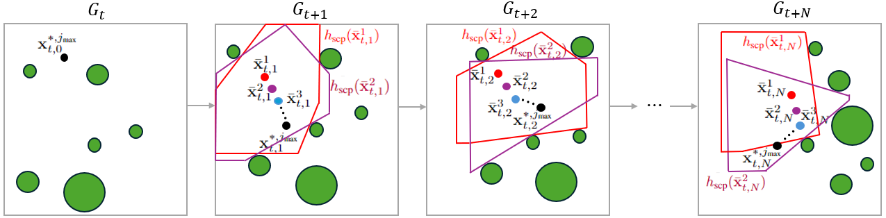
Figure 2: A schematic diagram illustrating how to find the open-loop trajectory (depicted by black points) based on SCP in sequential grip maps at time step $t$. Note that polygons of each color are generated based on the points of the corresponding color, and points in the next iteration can only be generated within the polygon created in the current iteration.

In Secs. III-C and III-D, we have illustrated the linearization of system dynamics as well as the process to get linear DCBFs. This approach enables us to incorporate them as constraints within a convex MPC framework at every iteration, an approach we refer to as convex finite-time constrained optimization control (CFTOC) [3]. This is solved at iteration $j$ with optimization variables $\mathbf{U}_{t}^{j}=[\mathbf{u}_{t,0}^{j},\dots,\mathbf{u}_{t,N-1}^{j}]$ and $\Omega_{t,i}^{j,n}=[\omega_{t,0,i}^{j,n},\dots,\omega_{t,N,i}^{j,n}]$, where $i\in\{1,\dots,m_{\text{cbf}}\},n\in\{1,\dots,n_{\text{scp}}\}.$

  CFTOC of iMPC-DHOCBF at iteration $j$:

$$\min_{\mathbf{U}_{t}^{j},\Omega_{t,1}^{j,n},\dots,\Omega_{t,m_{\text{cbf}}}^{j,n}}p(\mathbf{x}_{t,N}^{j})+\sum_{k=0}^{N-1}q(\mathbf{x}_{t,k}^{j},\mathbf{u}_{t,k}^{j},\omega_{t,k,i}^{j,n})$$ (17a)

s.t. $$\mathbf{x}_{t,k+1}^{j}{-}\bar{\mathbf{x}}_{t,k+1}^{j}{=}A^{j}(\mathbf{x}_{t,k}^{j}-\bar{\mathbf{x}}_{t,k}^{j}){+}B^{j}(\mathbf{u}_{t,k}^{j}-\bar{\mathbf{u}}_{t,k}^{j}),$$ (17b)

$$\mathbf{u}_{t,k}^{j}\in\mathcal{U},\ \mathbf{x}_{t,k}^{j}\in\mathcal{X},\ \omega_{t,k,i}^{j,n}\in\mathbb{R},$$ (17c)

$$\tilde{\psi}_{i-1}^{n}(\mathbf{x}_{t,k}^{j})+\sum_{\nu=1}^{i}Z_{\nu,i}^{n}(1-\gamma_{i}^{n})^{k}\tilde{\psi}_{0}^{n}(\mathbf{x}_{t,\nu}^{j})\geq$$

$$\omega_{t,k,i}^{j,n}Z_{0,i}^{n}(1-\gamma_{i}^{n})^{k}\tilde{\psi}_{0}^{n}(\mathbf{x}_{t,0}^{j}),$$ (17d)

 

In the CFTOC, the linearized dynamics constraints in (11) and the DCBF constraints in (15) are enforced with constraints (17b) and  (17d) at each open loop time step $k\in\{0,\dots,N-1\}$. The state and input constraints are considered in (17c). The slack variables are left unconstrained because the optimization’s objective is to minimize deviation from the nominal DCBF constraints through a cost term $q(\cdot,\cdot,\omega_{t,k,i}^{j,n})$, while ensuring feasibility of the optimization, as discussed in [3]. It’s important to note that to uphold the safety guarantee provided by the DCBFs, the constraints (17d) are strictly enforced using $i\in\{0,\dots,m_{\text{cbf}}\},n\in\{1,\dots,n_{\text{scp}}\},$ where $Z_{\nu,i}^{n}\in\mathbb{R}$ is defined in (16) with $\nu\in\{0,..,i\}$. The optimal decision variables of (17) at iteration $j$ is a list of control input vectors as $\mathbf{U}_{t}^{*,j}=[\mathbf{u}_{t,0}^{*,j},\dots,\mathbf{u}_{t,N-1}^{*,j}]$ and a list of slack variable vectors as $\mathbf{\Omega}_{t,i}^{*,j}=[\Omega_{t,i}^{*,j,1},\dots,\Omega_{t,i}^{*,j,n_{\text{scp}}}]$ where $\Omega_{t,i}^{*,j,n}=[\omega_{t,0,i}^{*,j,n},\dots,\mathbf{\omega}_{t,N,i}^{*,j,n}].$ The CFTOC is solved iteratively in Alg. 1, i.e., in sequential grip maps $[G_{t},G_{t+1},\dots,G_{t+N}],$ we generate red polygons based on red points $(\bar{\mathbf{x}}_{t,k}^{1})$, the purple points $(\bar{\mathbf{x}}_{t,k}^{2})$ will be generated inside red polygons; based on purple points we generate purple polygons, and the blue points $(\bar{\mathbf{x}}_{t,k}^{3})$ will be generated inside purple polygons. Repeat this process once the convergence criteria or the maximum iteration number $j_{\text{max}}$ is reached, and the open-loop trajectory (black points $\mathbf{x}_{t,k}^{*,j_{\text{max}}}$) can be extracted as shown in Fig. 2.

IV Case Study and Simulations

In this section, we present numerical results to demonstrate the effectiveness of our proposed method through the application of a unicycle model. For iMPC-DHOCBF, we used OSQP [22] to solve the convex optimizations at all iterations. The simulator for grip-map animation was based on RViz in Robot Operating System (ROS) Noetic Ninjemys. We used a Linux desktop with Intel Core i9-13900H running c++ for all computations.

IV-A Numerical Setup

IV-A1 System Dynamics

Consider a discrete-time unicycle model in the form

$$\begin{bmatrix}x_{t+1}{-}x_{t}\\ y_{t+1}{-}y_{t}\\ \theta_{t+1}{-}\theta_{t}\\ v_{t+1}{-}v_{t}\end{bmatrix}{=}\begin{bmatrix}v_{t}\cos(\theta_{t})\Delta t\\ v_{t}\sin(\theta_{t})\Delta t\\ 0\\ 0\end{bmatrix}{+}\begin{bmatrix}0&0\\ 0&0\\ \Delta t&0\\ 0&\Delta t\end{bmatrix}\begin{bmatrix}u_{1,t}\\ u_{2,t}\end{bmatrix},$$ (18)

where $\mathbf{x}_{t}=[x_{t},y_{t},\theta_{t},v_{t}]^{T}$ captures the 2-D location, heading angle, and linear speed; $\mathbf{u}_{t}=[u_{1,t},u_{2,t}]^{T}$ represents angular velocity ($u_{1}$) and linear acceleration ($u_{2}$), respectively. The system is discretized with $\Delta t=0.01$. System (18) is subject to the following state and input constraints:

$$\begin{split}\mathcal{X}=\{\mathbf{x}_{t}\in\mathbb{R}^{4}:&[-50,-50,-10,-40]^{T}\leq\mathbf{x}_{t},\\ &\mathbf{x}_{t}\leq[50,50,10,40]^{T}\},\\ \mathcal{U}=\{\mathbf{u}_{t}\in\mathbb{R}^{2}:&[-15,-5]^{T}\leq\mathbf{u}_{t}\leq[15,5]^{T}\}.\end{split}$$ (19)

IV-A2 System Configuration

The initial state is $[-35,-35,\theta_{0},25]^{T},$ the target state is $[45,45,\theta_{t_{\text{sim}}},25]^{T},$ and the reference state vector at time step $t$ up to horizon $N$ is $\mathbf{x}_{r,t+k}=[x_{r,t+k},y_{r,t+k},\theta_{r,t+k},v_{r,t+k}]^{T},k\in\left\{1,\dots,N\right\}.$ We use the first path transformation method introduced in Sec. III-B, and set all reference speed $v_{r,t+k}=25.$ $\theta_{0},\theta_{t_{\text{sim}}},\theta_{r,t+k}$ are calculated by the $atan2(Y,X)$ where the values of $(Y,X)$ are from every pair of adjacent points on the optimal path $\pi_{t}$. The other reference vectors are $\mathbf{u}_{r}=[0,0]^{T}$ and $\omega_{r}=[1,1]^{T}$.

IV-A3 DHOCBF

We get each candidate DHOCBF $h_{n}(\mathbf{x}_{t,k}^{j}|\bar{\mathbf{x}}_{t,k}^{j})$ from SCP introduced in Sec. III-D and set $m_{\text{cbf}}=1.$ From (16), we have $Z_{0,1}=1$. The decay rate $\gamma_{1}^{n}$ is 0.1. The obstacle detection range (the side length of the blue dashed square in Fig. 1) is 40.

IV-A4 MPC Design

The cost function of the MPC problem consists of stage cost $q(\mathbf{x}_{t,k}^{j},\mathbf{u}_{t,k}^{j},\omega_{t,k,i}^{j,n})=\sum_{k=0}^{N-1}(||\mathbf{x}_{t,k}^{j}-\mathbf{x}_{r,t+k}||_{Q}^{2}+||\mathbf{u}_{t,k}^{j}-\mathbf{u}_{r}||_{R}^{2}+||\omega_{t,k,i}^{j,n}-\omega_{r}||_{S}^{2})$ and terminal cost $p(\mathbf{x}_{t,N}^{j})=||\mathbf{x}_{t,N}^{j}-\mathbf{x}_{r,t+N}||_{P}^{2}$, where $Q=P=[10000,10000,100,10]^{T},R=\mathcal{I}_{2}$ and $S=100000\cdot\mathcal{I}_{2}$.

IV-A5 Convergence Criteria

We use the following absolute and relative convergence functions as convergence criteria mentioned in Alg. 1:

$$\begin{split}e_{\text{abs}}(\mathbf{X}_{t}^{*,j},\mathbf{U}_{t}^{*,j})&=||\mathbf{X}^{*,j}-\bar{\mathbf{X}}^{*,j}||\\ e_{\text{rel}}(\mathbf{X}_{t}^{*,j},\mathbf{U}_{t}^{*,j},\bar{\mathbf{X}}_{t}^{j},\bar{\mathbf{U}}_{t}^{j})&=||\mathbf{X}^{*,j}-\bar{\mathbf{X}}^{*,j}||/||\bar{\mathbf{X}}^{*,j}||.\end{split}$$ (20)

The iterative optimization stops when $e_{\text{abs}}<\varepsilon_{\text{abs}}$ or $e_{\text{rel}}<\varepsilon_{\text{rel}}$, where $\varepsilon_{\text{abs}}=0.05$, $\varepsilon_{\text{rel}}=10^{-2}$ and the maximum iteration number is set as $j_{\text{max}}=3$.

IV-B Performance

IV-B1 Avoiding Convex-Shape Dynamic Obstacles

The area that 2-D map covers is a square with $[-50,-50]^{T}\leq[x,y]^{T}\leq[50,50]^{T}$, consisting of 1200 by 1200 grids. We generate 7 square-shaped dynamic obstacles, each with side randomly generated within $[3,6]$ and linear constant speed randomly generated within $[2,4]$. The radius of a circular unicycle is 2. To enable the robot to avoid obstacles, we inflated the outer boundary of the obstacles by the radius of the robot. Fig. 3 shows the snapshots and the robot can find and follow a safe path during the simulation with $t_{\text{sim}}=600$. The video showcases successful animations in tighter environments, featuring obstacles with side lengths ranging within $[1,2].$ To validate the computation speed at each time step and success rate of the algorithm, we altered the number of obstacles and the number of horizon, and set $t_{\text{sim}}=100$. We randomly generated the robot’s initial and target positions in the map, with initial and reference speeds randomly generated between 10 and 40. Simulation results in Tab. I indicate that our algorithm’s per-step computation speed increases with the horizon size, yet it maintains a relatively fast computation speed (less than 0.2 seconds per step). This computation speed could be further enhanced by employing methods such as parallel computing. The obstacle avoidance success rate based on different numbers of obstacles was calculated from 50 sets of experiments, measured $>85\%.$

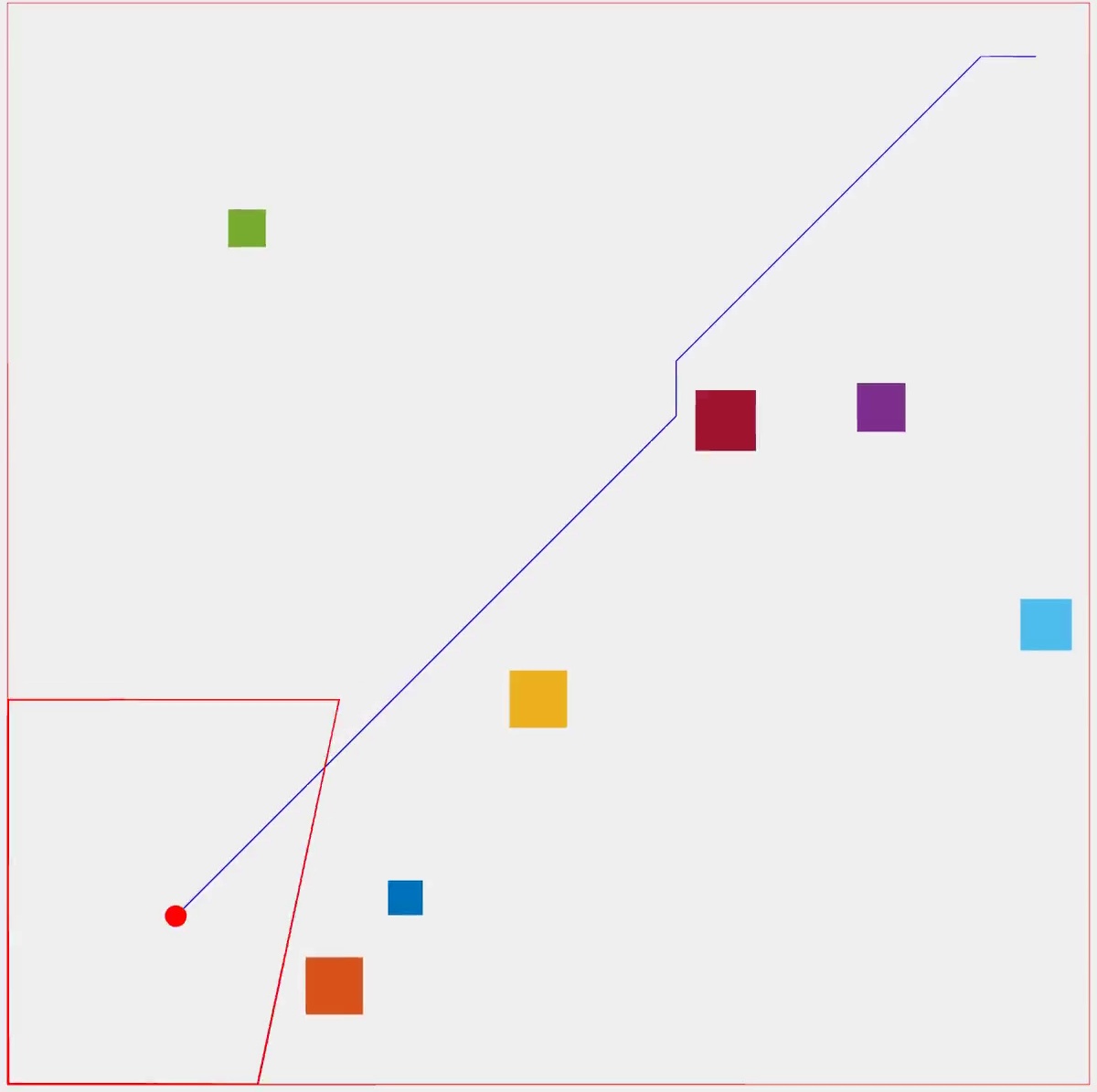
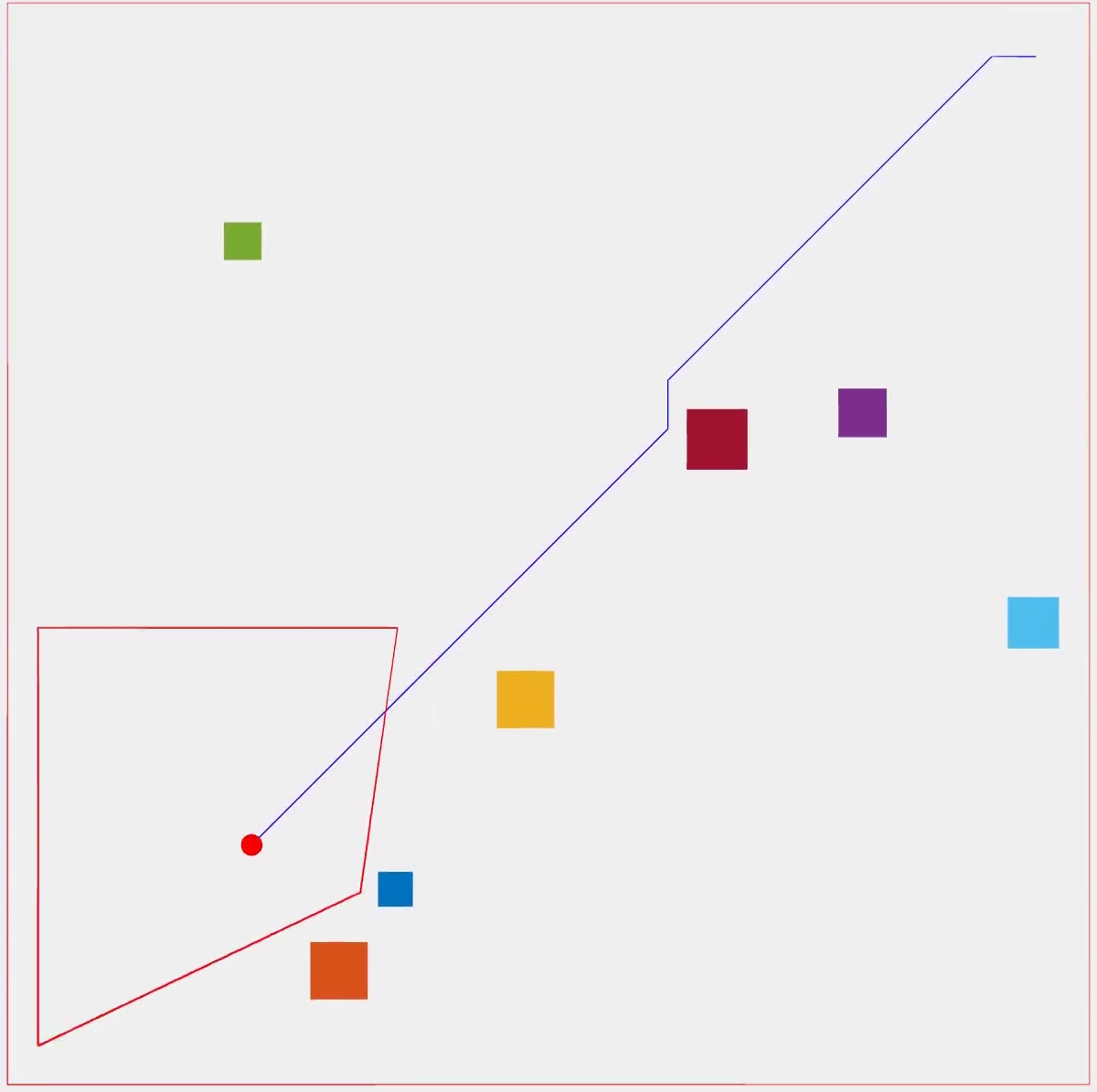
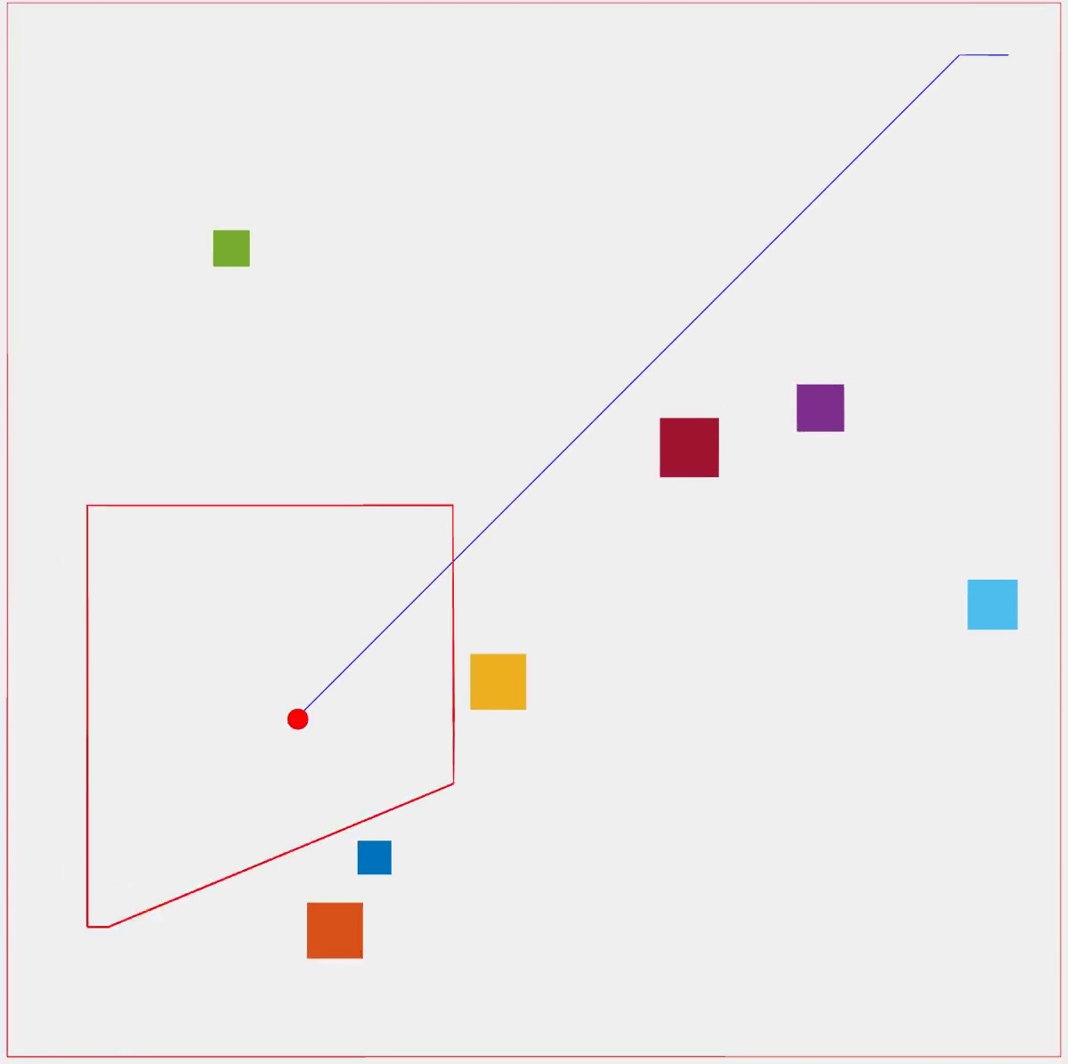
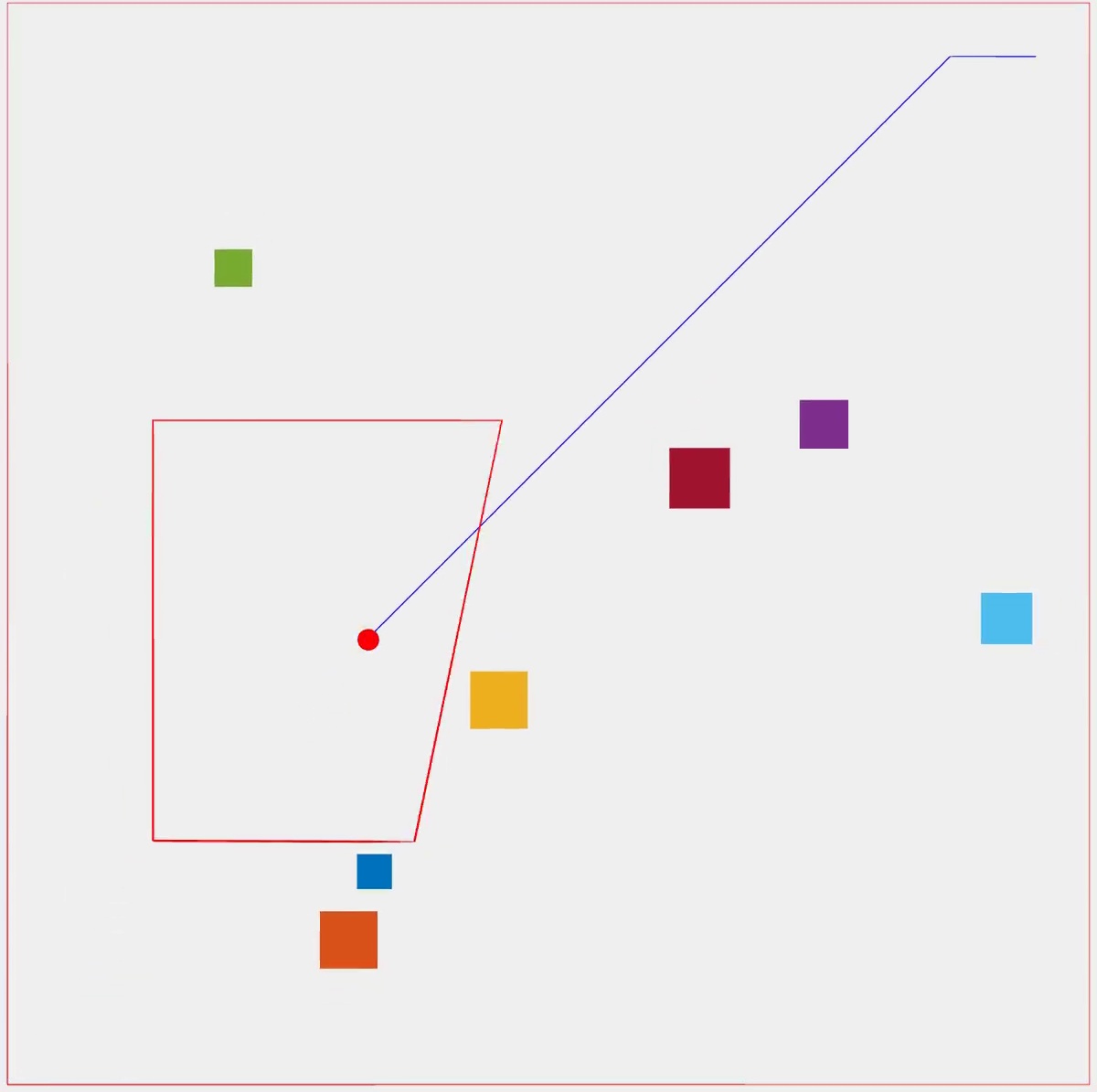
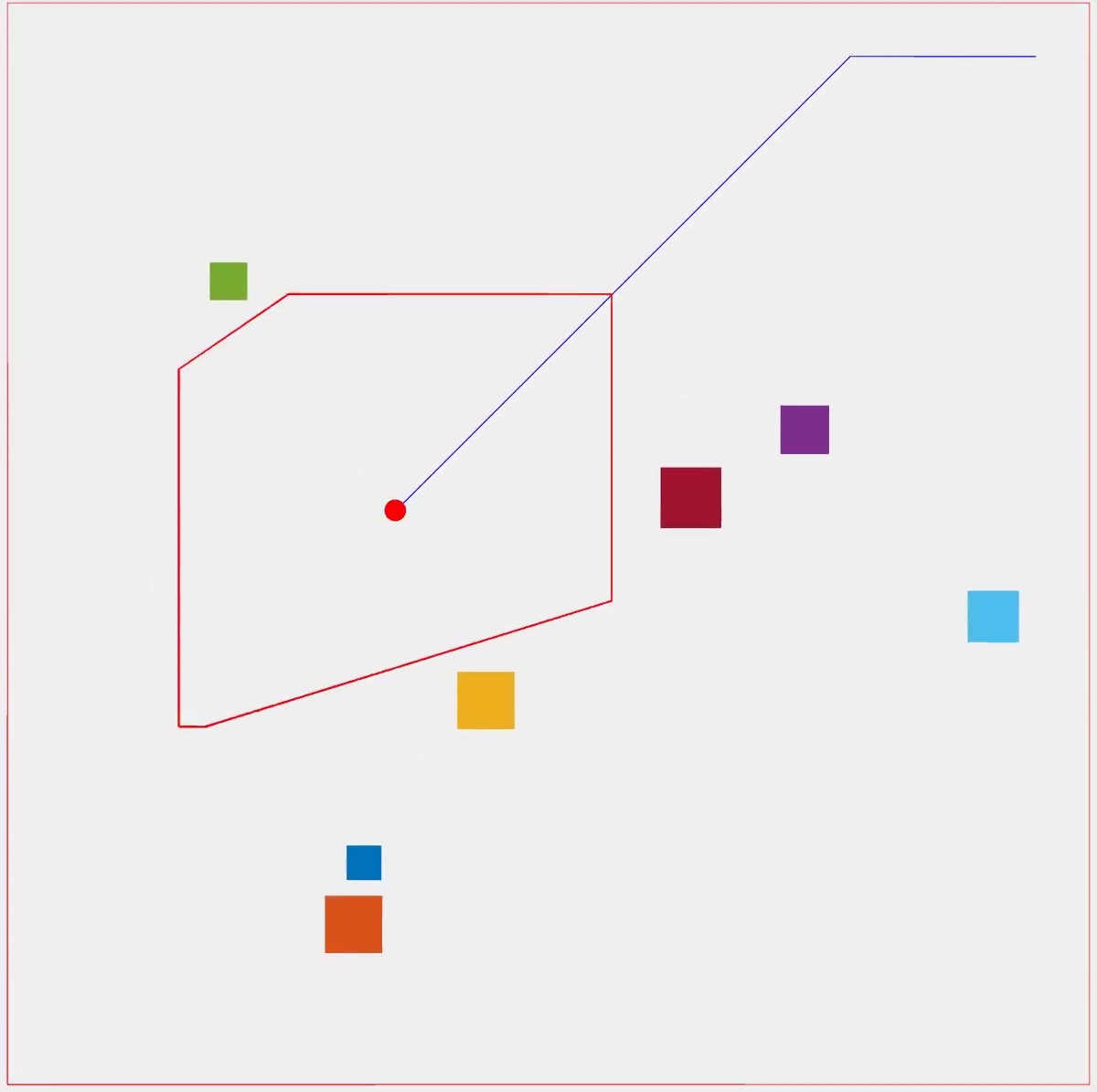
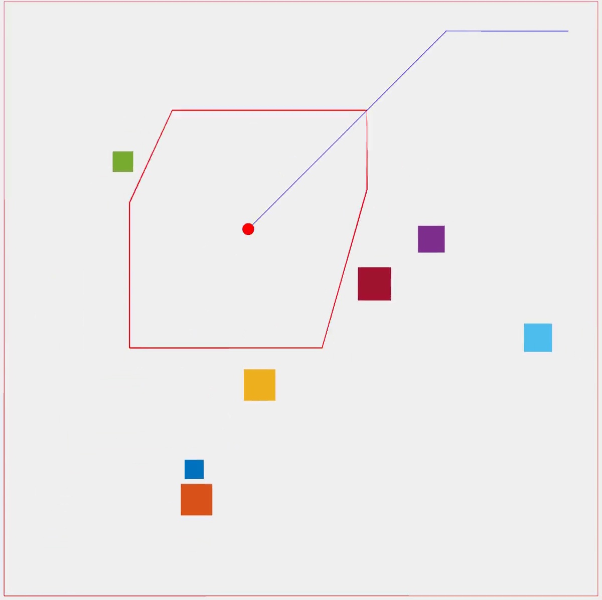
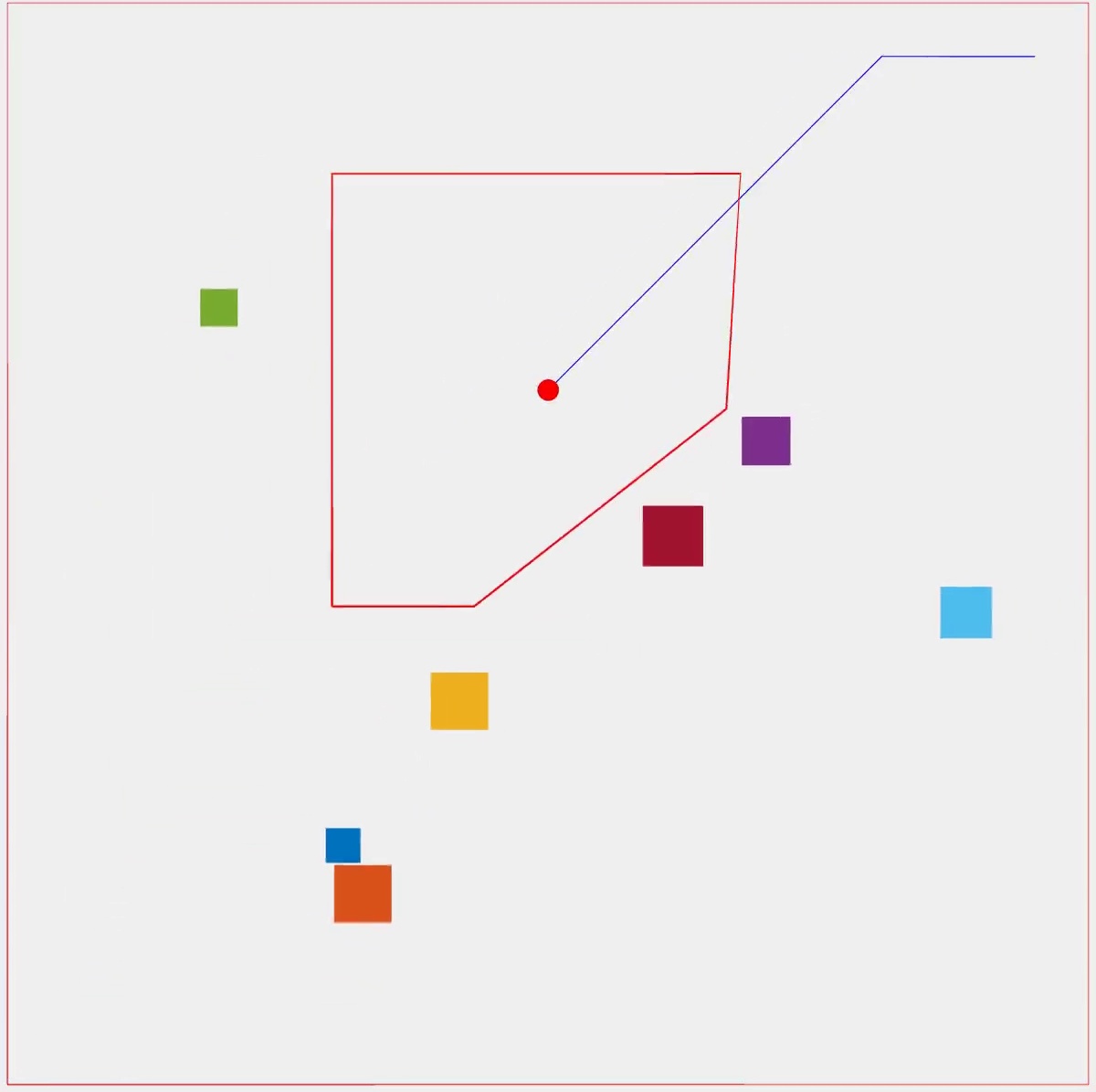
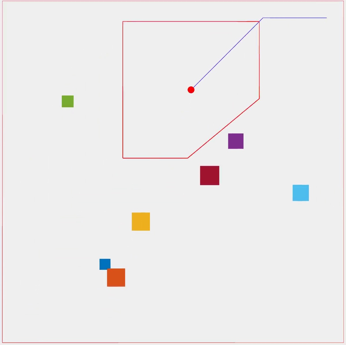
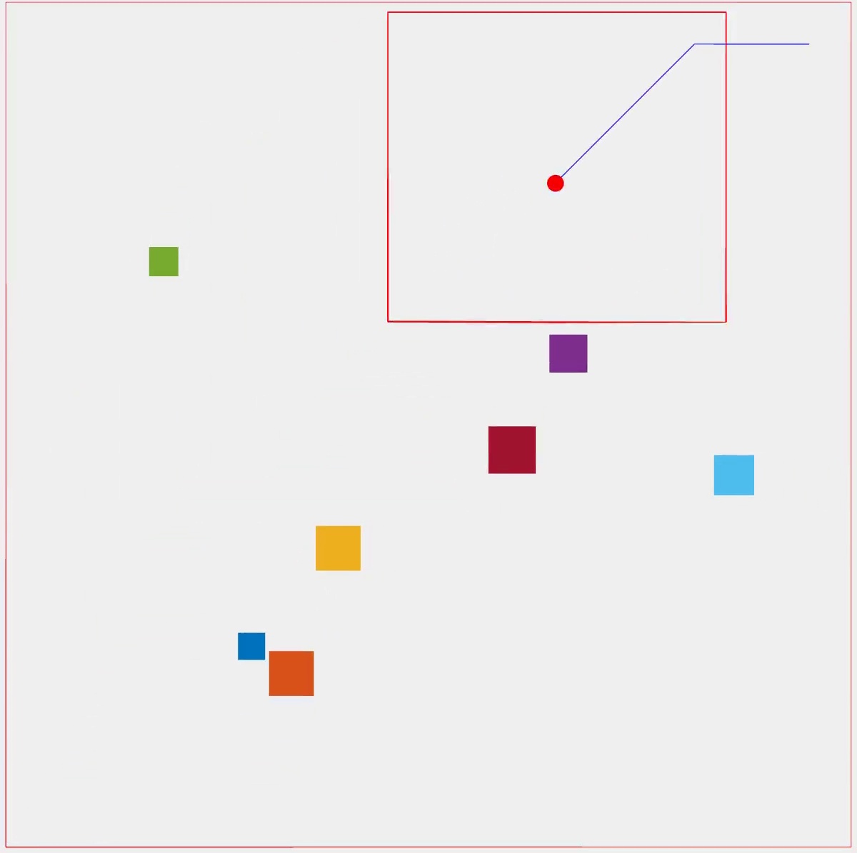
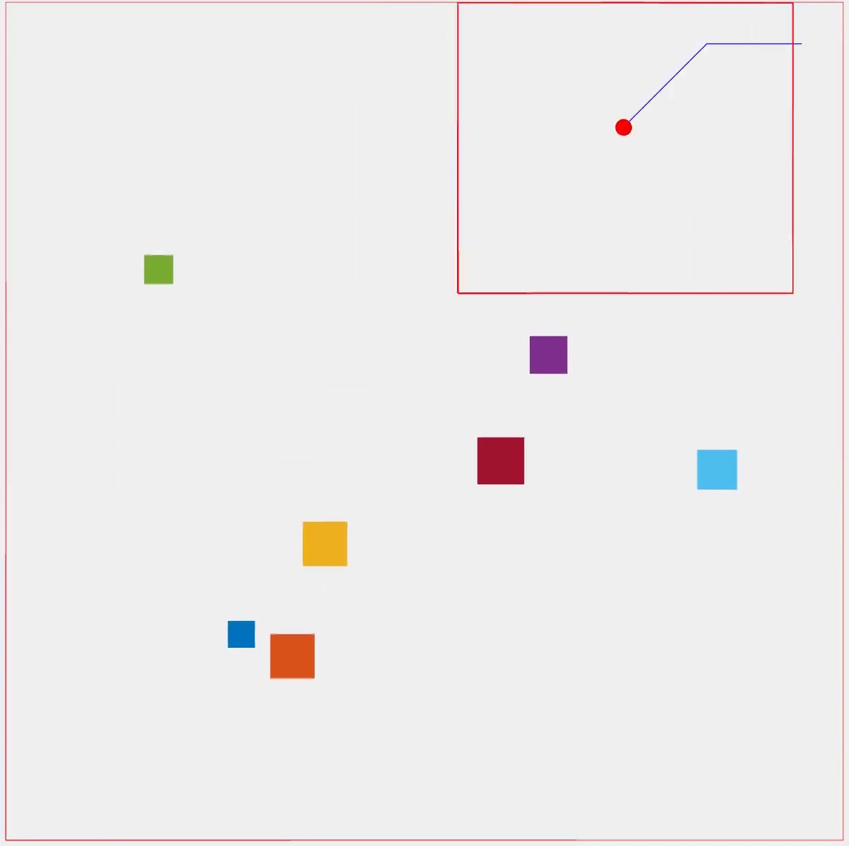
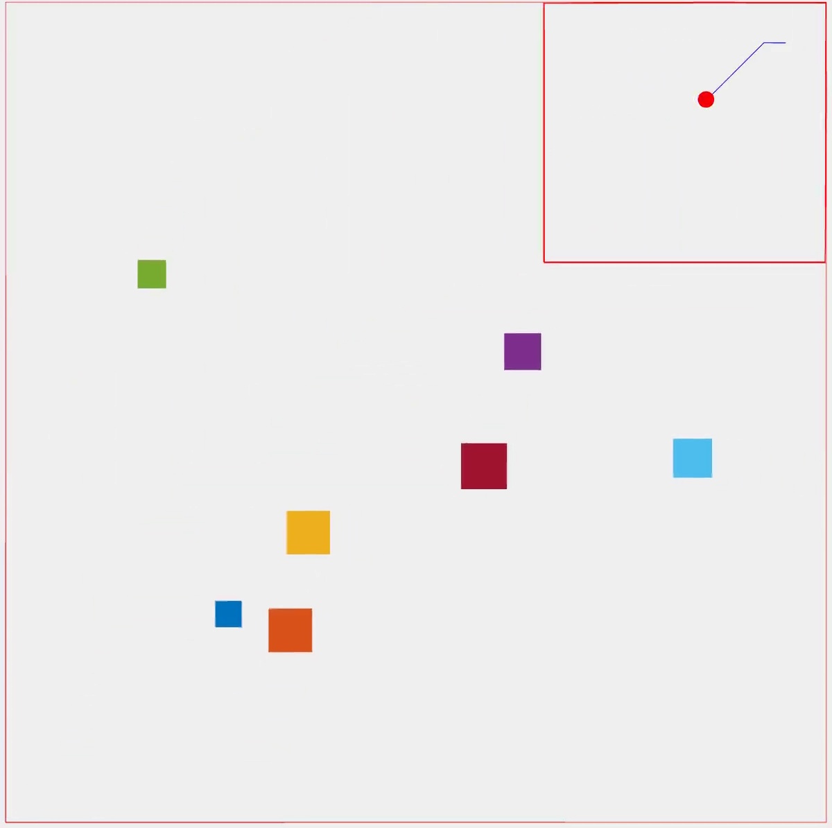
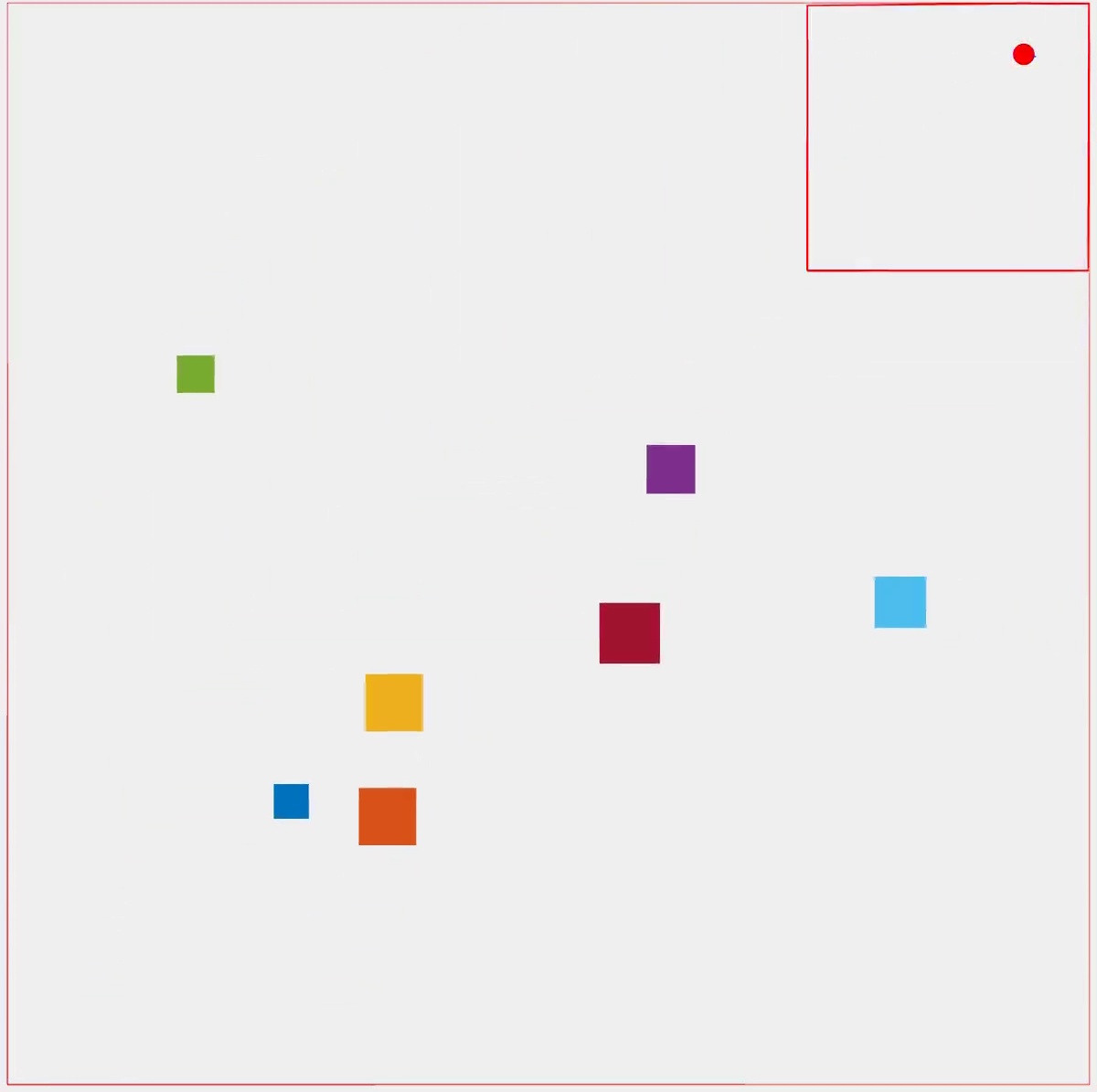
Figure 3: Snapshots from simulation of path (blue) and SCP (red polygon) found at specific time step of convex-shape dynamic obstacle avoidance (colorful squares) with a controlled robot (small red circle). The interval between each snapshot is 50 time steps and $N=20.$

Num of Obs	$N=4$	$N=12$	$N=20$	$N=20$
20	0.032s	0.100s	0.180s	$98\%$
30	0.036s	0.105s	0.193s	$90\%$
40	0.042s	0.108s	0.196s	$86\%$

TABLE I: Average computation speed at each time step (the middle three columns) and success rate (the last column) of the Alg. 1. $N$ denotes the number of horizon.

IV-B2 Avoiding Nonconvex-Shape Dynamic Obstacles

To show that our proposed algorithm works in a more complicated map, we generate 3 rotating windmills, each with 3 equal-length blades. The size of each blade measures $1*7$ and the angle between two adjacent blades is $\frac{2\pi}{3}.$ We randomly generate the constant translational speed of the blade’s geometric center within $[0,5]$, and the constant rotational speed of the blades is randomly generated within $[0,6]$. The radius of a circular unicycle is 2. Fig. 4 shows the snapshots. Additional animations are available in the video, featuring obstacles with rotation speeds ranging within $[0,12].$ In these animations, the robot can always find and follow a safe path during the simulation with $t_{\text{sim}}=600,$ even the space allowed for the robot to pass through is often very narrow.

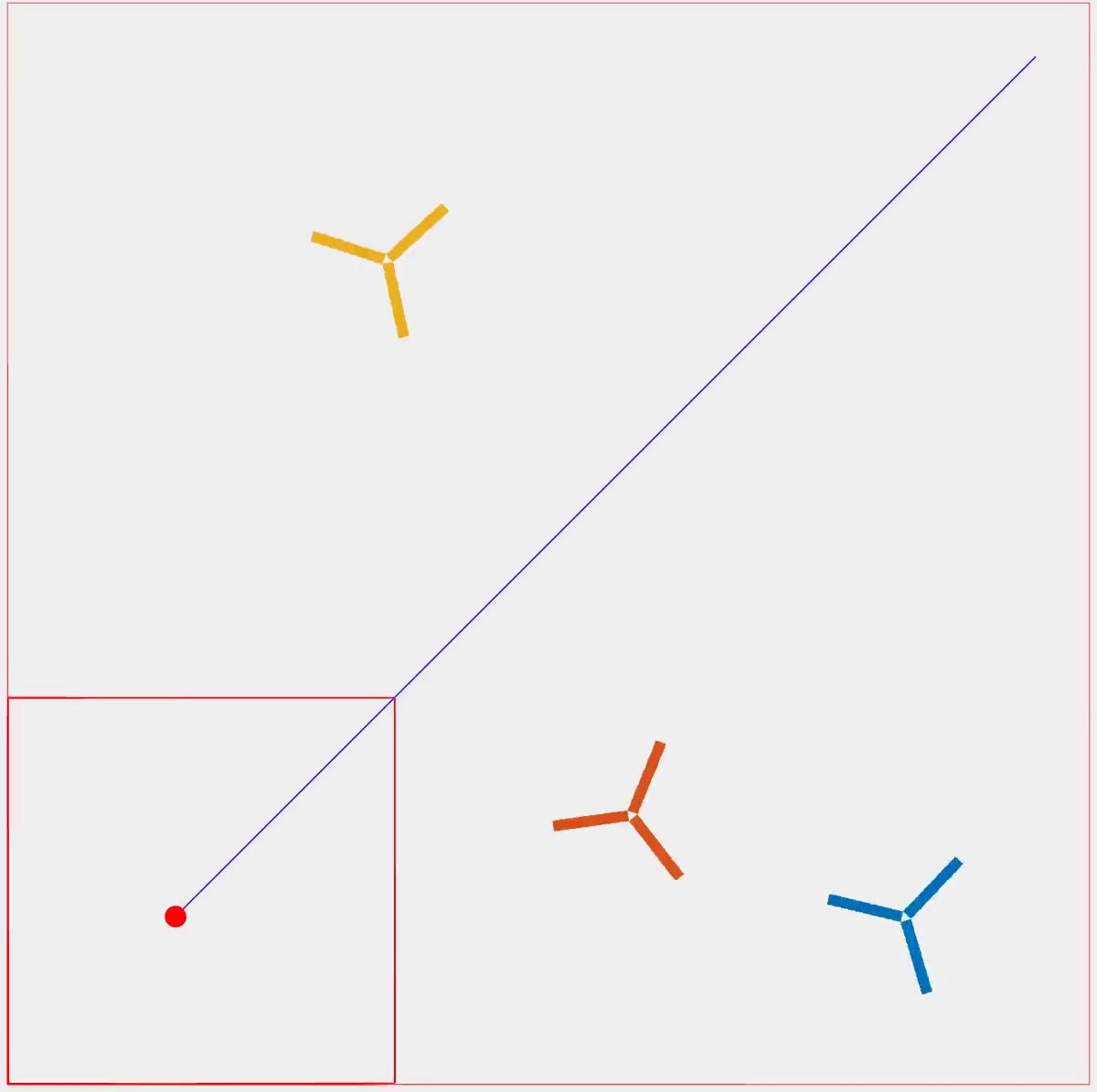
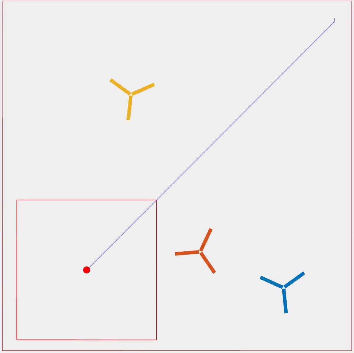
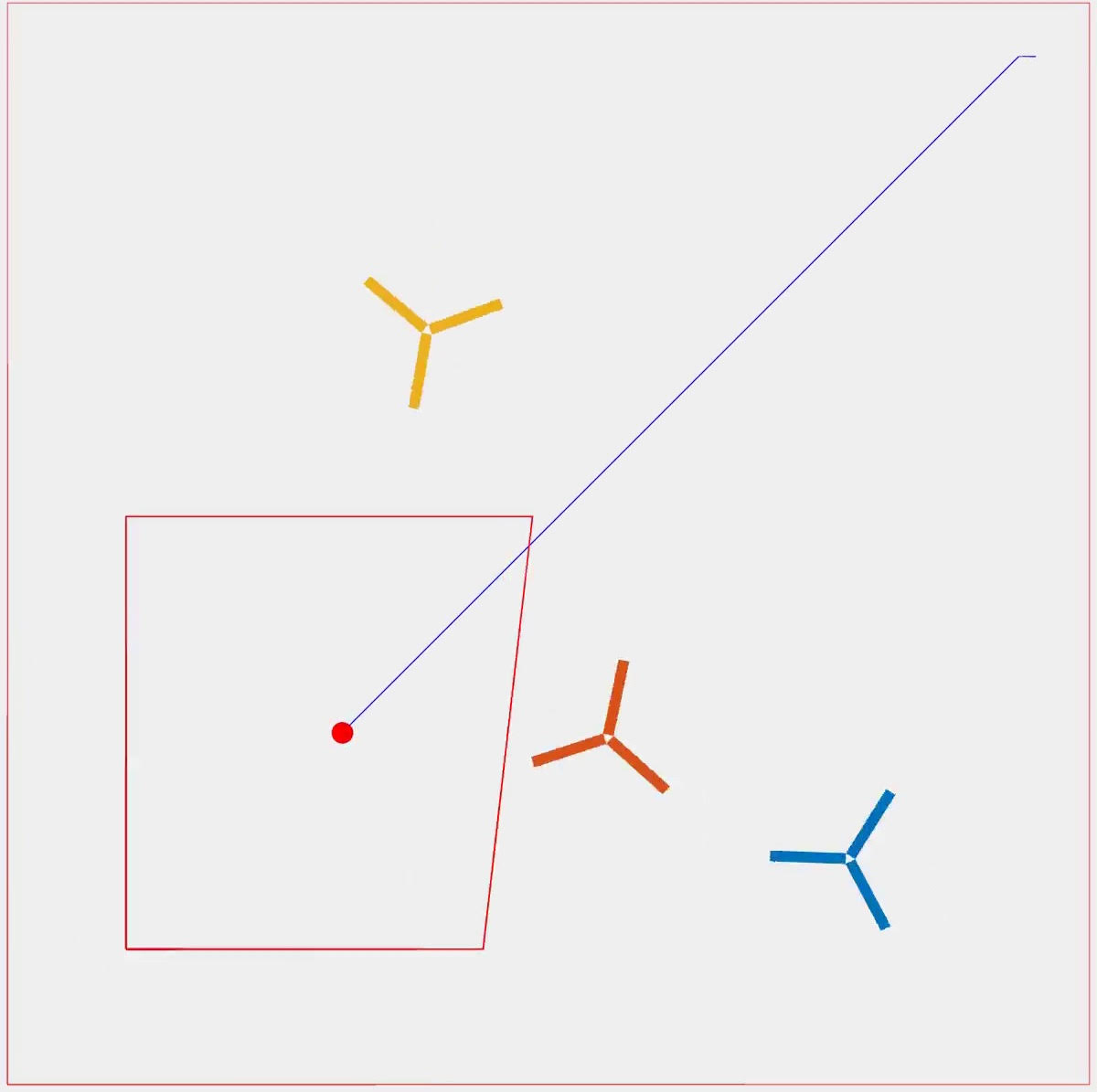
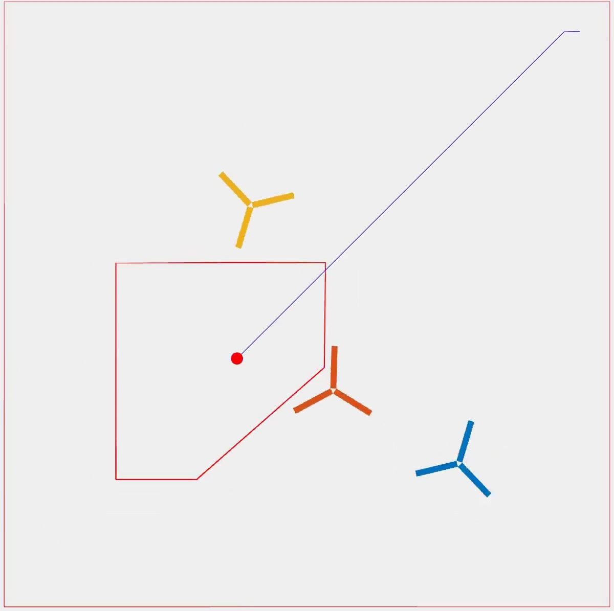
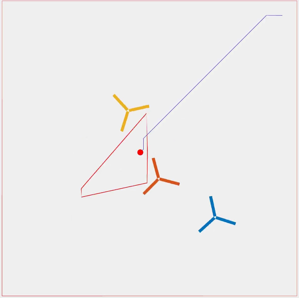
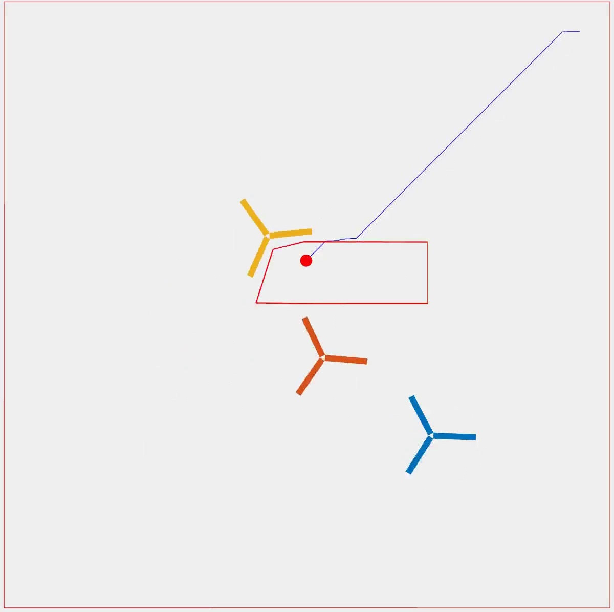
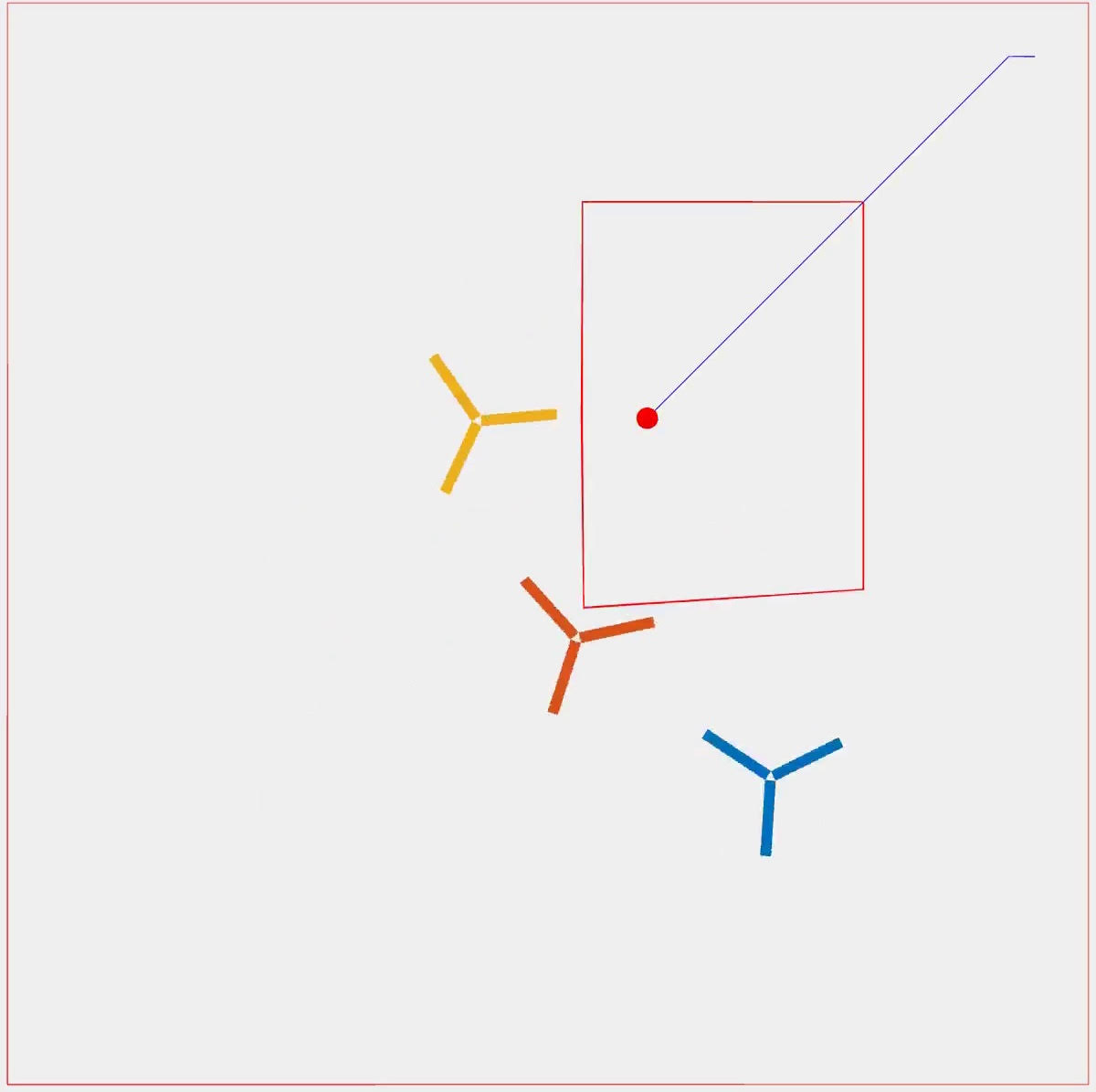
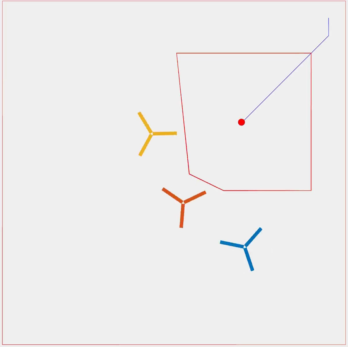
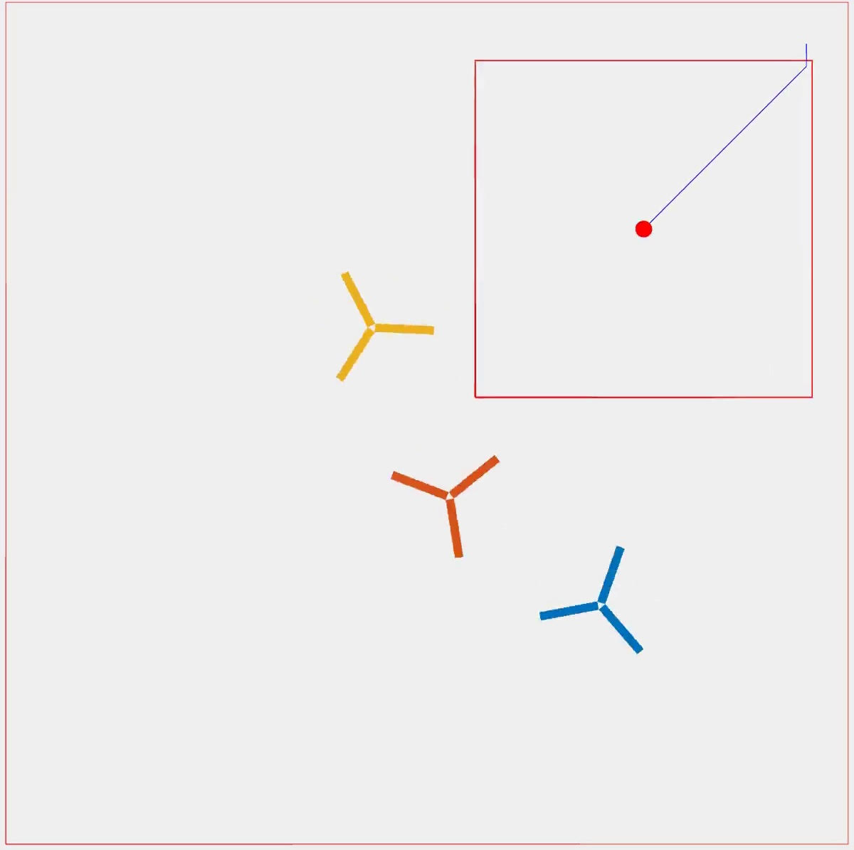
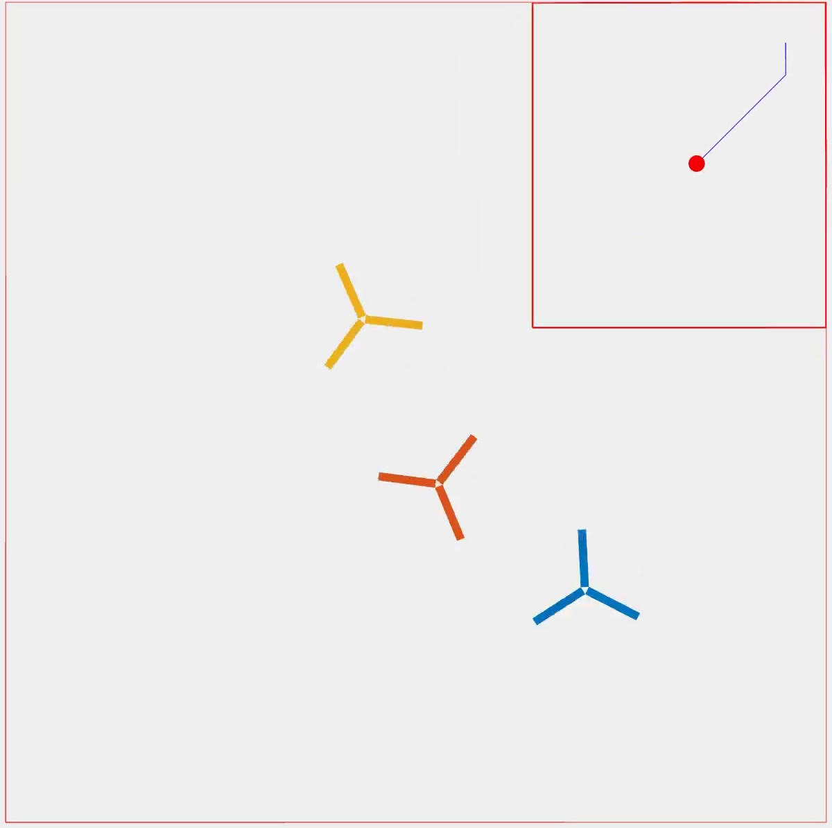
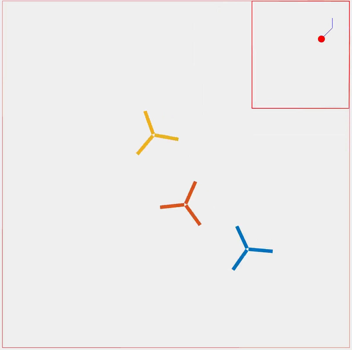
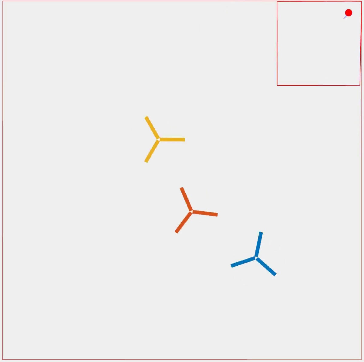
Figure 4: Snapshots from simulation of path (blue) and SCP (red polygon) found at specific time step of nonconvex-shape dynamic obstacle avoidance (colorful windmills) with a controlled robot (small red circle). The interval between each snapshot is 50 time steps and $N=20.$

V Conclusion and Future Work

We proposed an iterative convex optimization procedure using discrete-time control barrier functions for dynamic obstacle avoidance in grip maps. The proposed formulation has been shown to be applied as a rapid optimization for control and planning for general nonlinear dynamical systems. We validated our approach on navigation problems with obstacles of varying numbers, speeds, and shapes. There are still some scenarios the current method can not perfectly handle, i.e., the future information about dynamic obstacles in grid maps is unknown to us. We will address this limitation in future work.

References

• [1] A. D. Ames, J. W. Grizzle, and P. Tabuada, “Control barrier function based quadratic programs with application to adaptive cruise control,” in 53rd IEEE Conference on Decision and Control, 2014, pp. 6271–6278.
• [2] A. D. Ames, X. Xu, J. W. Grizzle, and P. Tabuada, “Control barrier function based quadratic programs for safety critical systems,” IEEE Transactions on Automatic Control, vol. 62, no. 8, pp. 3861–3876, 2016.
• [3] S. Liu, J. Zeng, K. Sreenath, and C. A. Belta, “Iterative convex optimization for model predictive control with discrete-time high-order control barrier functions,” in 2023 American Control Conference (ACC), 2023, pp. 3368–3375.
• [4] J. Zeng, Z. Li, and K. Sreenath, “Enhancing feasibility and safety of nonlinear model predictive control with discrete-time control barrier functions,” in 2021 60th IEEE Conference on Decision and Control (CDC), 2021, pp. 6137–6144.
• [5] S. Liu, M. Watterson, K. Mohta, K. Sun, S. Bhattacharya, C. J. Taylor, and V. Kumar, “Planning dynamically feasible trajectories for quadrotors using safe flight corridors in 3-d complex environments,” IEEE Robotics and Automation Letters, vol. 2, no. 3, pp. 1688–1695, 2017.
• [6] A. Agrawal and K. Sreenath, “Discrete control barrier functions for safety-critical control of discrete systems with application to bipedal robot navigation.” in Robotics: Science and Systems, vol. 13.   Cambridge, MA, USA, 2017.
• [7] J. Zeng, B. Zhang, Z. Li, and K. Sreenath, “Safety-critical control using optimal-decay control barrier function with guaranteed point-wise feasibility,” in 2021 American Control Conference (ACC), 2021, pp. 3856–3863.
• [8] R. Grandia, A. J. Taylor, A. D. Ames, and M. Hutter, “Multi-layered safety for legged robots via control barrier functions and model predictive control,” in 2021 IEEE International Conference on Robotics and Automation (ICRA), 2021, pp. 8352–8358.
• [9] H. Ma, X. Zhang, S. E. Li, Z. Lin, Y. Lyu, and S. Zheng, “Feasibility enhancement of constrained receding horizon control using generalized control barrier function,” in 2021 4th IEEE International Conference on Industrial Cyber-Physical Systems (ICPS), 2021, pp. 551–557.
• [10] Y. Xiong, D.-H. Zhai, M. Tavakoli, and Y. Xia, “Discrete-time control barrier function: High-order case and adaptive case,” IEEE Transactions on Cybernetics, pp. 1–9, 2022.
• [11] S. He, J. Zeng, and K. Sreenath, “Autonomous racing with multiple vehicles using a parallelized optimization with safety guarantee using control barrier functions,” in 2022 International Conference on Robotics and Automation (ICRA), 2022, pp. 3444–3451.
• [12] Z. Li, J. Zeng, A. Thirugnanam, and K. Sreenath, “Bridging model-based safety and model-free reinforcement learning through system identification of low dimensional linear models,” in Proceedings of Robotics: Science and Systems, 2022.
• [13] G. Paolo, I. Ferrara, and L. Magni, “Mpc for robot manipulators with integral sliding mode generation,” IEEE/ASME Transactions on Mechatronics, vol. 22, no. 3, pp. 1299–1307, 2017.
• [14] N. Scianca, D. De Simone, L. Lanari, and G. Oriolo, “Mpc for humanoid gait generation: Stability and feasibility,” IEEE Transactions on Robotics, vol. 36, no. 4, pp. 1171–1188, 2020.
• [15] T. D. Son and Q. Nguyen, “Safety-critical control for non-affine nonlinear systems with application on autonomous vehicle,” in 2019 IEEE 58th Conference on Decision and Control (CDC), 2019, pp. 7623–7628.
• [16] J. M. Eklund, J. Sprinkle, and S. S. Sastry, “Switched and symmetric pursuit/evasion games using online model predictive control with application to autonomous aircraft,” IEEE Transactions on Control Systems Technology, vol. 20, no. 3, pp. 604–620, 2012.
• [17] J. V. Frasch, A. Gray, M. Zanon, H. J. Ferreau, S. Sager, F. Borrelli, and M. Diehl, “An auto-generated nonlinear mpc algorithm for real-time obstacle avoidance of ground vehicles,” in 2013 European Control Conference (ECC), 2013, pp. 4136–4141.
• [18] A. Liniger, A. Domahidi, and M. Morari, “Optimization-based autonomous racing of 1: 43 scale rc cars,” Optimal Control Applications and Methods, vol. 36, no. 5, pp. 628–647, 2015.
• [19] X. Zhang, A. Liniger, and F. Borrelli, “Optimization-based collision avoidance,” IEEE Transactions on Control Systems Technology, vol. 29, no. 3, pp. 972–983, 2020.
• [20] D. Harabor and A. Grastien, “Online graph pruning for pathfinding on grid maps,” in Proceedings of the AAAI conference on artificial intelligence, vol. 25, no. 1, 2011, pp. 1114–1119.
• [21] M. Sun and D. Wang, “Initial shift issues on discrete-time iterative learning control with system relative degree,” IEEE Transactions on Automatic Control, vol. 48, no. 1, pp. 144–148, 2003.
• [22] B. Stellato, G. Banjac, P. Goulart, A. Bemporad, and S. Boyd, “Osqp: An operator splitting solver for quadratic programs,” Mathematical Programming Computation, vol. 12, no. 4, pp. 637–672, 2020.