Nonstandard Lagrangians and branched Hamiltonians: A brief review
Abstract
Time and again, non-conventional forms of Lagrangians have found attention in the literature. For one thing, such Lagrangians have deep connections with several aspects of nonlinear dynamics including specifically the types of the Liénard class; for another, very often the problem of their quantization opens up multiple branches of the corresponding Hamiltonians, ending up with the presence of singularities in the associated eigenfunctions. In this article, we furnish a brief review of the classical theory of such Lagrangians and the associated branched Hamiltonians, starting with the example of Liénard-type systems. We then take up other cases where the Lagrangians depend upon the velocity with powers greater than two while still having a tractable mathematical structure, while also describing the associated branched Hamiltonians for such systems. For various examples, we emphasize upon the emergence of the notion of momentum-dependent mass in the theory of branched Hamiltonians.
I Introduction
During the past few years, the study of non-conventional types of dynamical systems, in particular those which are controlled by Lagrangians that are not quadratic in the velocity has entered a new phase of intense development SW ; SW1 ; SW2 ; MCZ . Such Lagrangians lead to certain exotic Hamiltonians, commonly termed as branched Hamiltonians, that have relevance in their applicability to problems of nonlinear dynamics pertaining to autonomous differential equations bspf ; mitso , and to certain exotic quantum-mechanical models especially in the context of non-hermitian parity-time ()-symmetric schemes bender , along with their relativistic counterparts bpm .
A simple way to see how Lagrangians that are not quadratic in the velocity can lead to sensible dynamical systems is to consider the following toy model benoy ; carinena :
| (1) |
where and are real numbers satisfying , and . Notice that the Lagrangian cannot be expressed as the difference between the kinetic and potential energies; such Lagrangians shall be referred to as nonstandard. A direct computation reveals that the Euler-Lagrange equation is
| (2) |
where and . Eq. (2) is just the harmonic oscillator in the presence of linear damping. We remind the reader that there is no time-independent Lagrangian of the ‘standard’ kind from which one can reproduce Eq. (2) upon invoking the Euler-Lagrange equation444One could recover the damped oscillator from a standard Lagrangian by using a Rayleigh dissipation function goldsteincm . Alternatively, one can consider the modified Euler-Lagrange equations from the Herglotz variational problem to describe the damped oscillator herglotz . We do not consider such situations here.. There exist various other families of nonstandard Lagrangians (giving rise to different dynamical systems) which look quite different from Eq. (1); each family is endowed with their own intriguing features. However, the common theme is the existence of Lagrangians that are not quadratic in the velocity, thereby leading to a nonlinear relationship between the velocity and the momentum. This leads to the notion of branching, typically yielding the so-called Riemann-surface phase-space structure and in consequence, certain interesting topological features CZ1 .
In the classical context, the problems associated with branched Hamiltonians and the ones that are inevitably posed after their quantization, were addressed by Shapere and Wilczek SW ; SW1 ; SW2 . This has triggered off a series of papers by Curtright and Zachos CZ1 ; CZ2 ; CZ3 ; CZ4 ; CZ ; C1 which were subsequently followed up by other works in a similar direction (see for example, Refs. bspf ; bst ; agp ). It bears mention that local branching is not so sufficient to ensure
integrability. In particular, finding an integrable differential equation having
solutions that are not locally finitely branched with a finitely-sheeted Riemann surface but
not yet identified through Painlevé analysis, is in itself an interesting open problem CZ1 .
Against this background, a new class of innovations
on the description and simulations of quantum dynamics emerged in relation to the specific role played by certain models constructed appropriately. Not quite unexpectedly, Hamiltonians which are multi-valued functions of momenta confront us with some typical insurmountable ambiguities of quantization. In such cases, the underlying
Lagrangian possesses time derivatives in excess of quadratic powers (or sometimes, inverse powers). The use of
these models leads, on both classical and quantum grounds, to the necessity of a re-evaluation
of the dynamical interpretation of the momentum, which, in principle, becomes a multi-valued
function of velocity. It also needs to be pointed out that the
traditional approaches often do not always work as is the case with
certain -symmetric complex potentials possessing real spectra BagG or, on employing tractable non-local generalizations zno1 .
There have been efforts to construct simple systems with toy Lagrangians that lead to multi-valued Hamiltonian systems. Such Hamiltonians would be defined in the momentum space revealing
systems with momentum-dependent masses BGG ; agp ; brp .
In the context of nonlinear models, the Liénard system presents an intriguing feature
of the Hamiltonian in which the roles of the position and
momentum variables often get exchanged BGG ; ML . Thus, Liénard systems are of potential importance in optics DOR as well as in non-Hermitian quantum mechanics BGG ; Bag2 .
Naturally, the presence of the
damping as is the case for Liénard systems poses to be a problem whenever one tries to contemplate a quantization of the
model.
It is important to realize that the quantization is hard to tackle in the coordinate representation of the Schrödinger equation but can be straightforwardly carried out in the momentum space. Such a Hamiltonian, which has a branched character, may be interpreted to represent an effective-mass quantum
system BGG ; Roos ; ruby .
Although much has been said about the quantum-mechanical formalisms, in this paper, we focus on the classical theory, (briefly) reviewing some aspects of nonstandard Lagrangians and the associated branched Hamiltonians. The theory is exemplified by focusing on various examples which include some systems of the Liénard class, which are of great interest in the theory of dynamical systems. Apart from Liénard systems, we discuss some interesting toy Lagrangians which contain time derivatives in excess of quadratic powers, leading to branched Hamiltonians. The basic features of the theory are discussed in the light of these examples. However, we begin with a discussion on some simple nonstandard Lagrangians which can be figured out via some guesswork; we call them trial Lagrangians and they are discussed in Section II. Following this, in Section III we discuss nonstandard Lagrangians and branched Hamiltonians in the context of Liénard systems, wherein we outline a systematic derivation of the Lagrangians, provided the system admits a certain integrability condition. In Sections IV, V and VI we analyze various intriguing examples of Lagrangians in which time derivatives occur in excess of quadratic powers, while also discussing the associated Hamiltonians. We conclude with some remarks in Section VII where, in particular, a few further aspects of the problem of quantization are discussed. .
II Trial Lagrangians: Reciprocal and logarithmic kinds
Sometimes one can make educated guesses to construct plausible nonstandard Lagrangians. We cite a few examples.
Example 1 – Consider the following Lagrangian benoy ; carinena :
| (3) |
where is a well-behaved function (typically a polynomial), while and are real-valued and non-zero constant numbers. Obviously, it does not reveal the ‘standard’ form as the difference between the kinetic and potential energies. However, the Euler-Lagrange equation gives , with and , where for instance, picking gives the linearly-damped harmonic oscillator, while the choice implies and . Lagrangians of this type [Eq. (3)] are termed as reciprocal Lagrangians.
Example 2 – Consider another form of Lagrangians classified by benoy
| (4) |
where and are real-valued and non-zero constant numbers. The Euler-Lagrange equation goes as , with and . Lagrangians given by Eq. (4) are termed as logarithmic Lagrangians.
Example 3 – As another example, we point out that some equations that go as , where and are suitable functions of can be derived from (reciprocal) Lagrangians that read
| (5) |
such that . Specifically, the functions and are
| (6) |
| (7) |
However, there is a limited variety of differential equations that can be described by Lagrangians which may be guessed; in general, it is often not possible to systematically derive a Lagrangian from which the equation may emerge as the Euler-Lagrange equation. In what follows, we describe Liénard systems and demonstrate that if a certain integrability condition is satisfied, then one may systematically find nonstandard Lagrangians describing such systems.
III Liénard systems
A Liénard system is a second-order ordinary differential equation that goes as
| (8) |
where555Often it is sufficient to have . can be suitably chosen. Interesting choices for and include and , which is just the damped linear oscillator, while the choice and gives the van der Pol oscillator, known to admit limit-cycle behavior due to the particular choice of str . Another choice is and , for which we have the linearly-damped (nonlinear) Duffing oscillator. It is noteworthy that in any case with , the system exhibits non-conservative dynamics because Eq. (8) does not stay invariant under the transformation , namely, time reversal. Further, oscillatory dynamics can be obtained if is an even function and if is odd; it follows from the fact that the overall force (the second and third terms of Eq. (8)) should be odd under in order to support oscillations mic .
III.1 Cheillini condition and nonstandard Lagrangians
We now discuss a systematic derivation of nonstandard Lagrangians describing certain Liénard systems agp ; BGG . The idea is to make use of a function known as the Jacobi last multiplier which may be defined as follows whittaker . Given a second-order ordinary differential equation,
| (9) |
one defines the last multiplier as a solution of the following differential equation:
| (10) |
As has been discussed in Whittaker’s classic textbook whittaker , if a second-order differential equation such as Eq. (9) follows from the Euler-Lagrange equations, then the Lagrangian is related to the last multiplier as
| (11) |
This allows one to determine the Lagrangian function for a given second-order differential equation, provided it admits a Lagrangian formalism. For the Liénard system, a formal solution for the last multiplier is found to be
| (12) |
where is some nonlocal variable and is a suitable parameter whose significance appears in the following lemma:
Lemma 1
The Liénard equation [Eq. (8)] can be written as the following system of first-order equations:
| (13) |
where , with the parameter being determined by the following condition:
| (14) |
Proof - From Eq. (12) we have
| (15) |
which means . Simply putting , we find by differentiating with respect to , the following expression:
| (16) |
Thereafter, substituting the expression for from the previous equation and after eliminating , it follows that
| (17) |
Comparison with Eq. (8) reveals that one must choose
and . Consistency between these two choices therefore demands that the condition appearing in Eq. (14) should be fulfilled.
It is noteworthy that Eq. (14) represents what is known as the Cheillini condition, allowing one to recast the Liénard system in the form suggested in Eq. (13). Specifically, if , then Eq. (14) dictates that must satisfy the following differential equation:
| (18) |
A simple integration gives
| (19) |
where is an integration constant. This gives the functional form of so as to satisfy the Cheillini condition. In the cases where the Cheillini condition is satisfied, one can find the Lagrangian as follows:
Theorem 1
Consider a Liénard system with choices of and that satisfy the Cheillini condition. Then, the second-order differential equation can be obtained as the Euler-Lagrange equation of the Lagrangian that reads
| (20) |
Proof - If the functions and satisfy Eq. (14), then we have from Eqs. (11) and (12), the following condition:
| (21) |
Then, it follows straightforwardly by simple integration that the Lagrangian is given by Eq. (20). Clearly, a Lagrangian such as the one appearing in Eq. (20) is of the nonstandard form because there is no identification of kinetic and potential energies. It may be emphasized that not all choices of and would satisfy the Cheillini condition, meaning that such equations cannot be cast into the form of Eq. (13); an example is the van der Pol oscillator for which and . Therefore, not all Liénard systems are known to admit a Lagrangian description.
III.2 Hamiltonian aspects
Now that we are equipped with the Lagrangian that describes the Liénard system, we can move on to its Hamiltonian aspects. The conjugate momentum is found to be
| (22) |
Thus, the expression may be multi-valued, depending upon . It goes as
| (23) |
where is some function of and is a constant. Using the above form, the Hamiltonian is found to be
| (24) |
Notice that if Eq. (23) admits branching, then so does the Hamiltonian [Eq. (24)]. Below, we discuss a concrete example.
III.3 A concrete example
We discuss an example now, which will help us understand the framework discussed above. In particular, we will also encounter the notion of momentum-dependent mass BGG ; brp ; ML , a concept that has generated some interest in the recent times, especially within the quantum-mechanical framework. We consider the case where and agp ; Eq. (14) is satisfied for . We consider each case separately now.
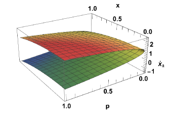
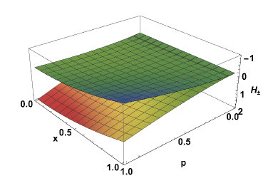
III.3.1 Case with
In the case where , we have
| (25) |
which points towards branching. Notice that branching originates from the nonlinear dependence between and in the equation . The corresponding branched Hamiltonians turn out to be
| (26) |
exhibiting two distinct branches, where . We have plotted the function in Fig. (1), while Fig. (2) shows a plot of the branched pair of Hamiltonians, . The branches coalesce at .
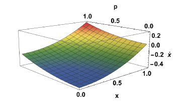
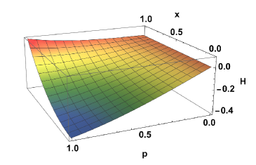
III.3.2 Case with
In the case where , we have
| (27) |
implying that there is no branching, because can be solved uniquely as a function of the momentum. A straightforward calculation reveals that the Hamiltonian turns out to be
| (28) |
wherein, there is only one branch. In Figs. (3) and (4), we have plotted and . An intriguing aspect of the Hamiltonian given in Eq. (28) is that it may be expressed as
| (29) |
This resembles a standard Hamiltonian with the roles of coordinate and momentum being interchanged; its then tempting to interpret as a momentum-dependent mass. The quantization of such systems proceeds in the momentum space, often with the notion of momentum-dependent mass (see for example, Ref. BGG ).
IV The model
Shapere and Wilczek have discussed a concrete model depicting a non-convex nature of the Lagrangian which reads SW
| (30) |
where is the velocity666Now and in subsequent discussions, we will denote . and is a coupling parameter. Corresponding to Eq. (30), the conjugate momentum is a cubic function in that is given by
| (31) |
Clearly, is not monotonic in velocity, which may lead to branching. The corresponding Hamiltonian is obtained as
| (32) |
which, like , is also a multi-valued function (with cusps) in the conjugate momentum , since each given corresponds to one or three values of as shown in Eq. (31).
Hence, for systems with a non-convex Lagrangian such as Eq. (30), the construction of the corresponding Hamiltonian in conjugate momentum variable is not unique. A similar incertitude is also encountered in cosmology models ctv ; nhm , in generalized schemes of Einstein gravity which involve topological invariants, and in theories of higher-curvature gravity ctj . We note in passing that if one is given a single-valued Lagrangian , and define it according to , rather than the usual form , and that if the or dependence is non-convex, then branched functions are always encountered, as a result of employing the Legendre transformation, despite having started with a single-valued Lagrangian or Hamiltonian function.
V A generalized class of Lagrangians and branched Hamiltonians
V.1 Velocity-independent potentials
Curtright and Zachos CZ extended the analysis of SW by considering a generalized class of non-quadratic Lagrangians that go as
| (33) |
where the traditional kinetic-energy term is replaced by a fractional function of the velocity variable , and represents a convenient local-interaction potential. The fractional powers facilitate the derivation of supersymmetric partner forms of the potential á la Witten witt . We remark that the st
root of the first term in is required to be real, and or for or , respectively.
Let us focus on the case with . Performing a Taylor expansion for near zero, we can write . While the first term is merely a constant and the second term contributes to the boundary of the action and therefore does not influence the equations of motion, the third term yields the kinetic structure:
| (34) |
Thus, for small velocities, the action results in the usual Newtonian form of the equations of motion.
On the other hand, for large velocities, we have a rather nontrivial scenario which leads (for finite, positive-integer values of ) to a non-convex function of . The curvature term corresponding to the quantity changes sign at just the point . Thus, may be interpreted as a single pair of convex functions that have been judiciously pieced together. Now, from the Lagrangian given in Eq. , the canonical momentum can be easily calculated to be
| (35) |
Inverting the relation we observe at once that the velocity variable emerges as a double-valued function of :
| (36) |
Corresponding to the two signs above, a pair branches of the Hamiltonian, namely, will appear. Specifically, for any positive-integer value of , these may be identified to be
| (37) |
From a classical perspective, in order to avoid an imaginary , one needs to address a nonnegative . This in turn implies that the slope is always positive. It is interesting to note that for the case we are led to the quantum-mechanical supersymmetric structure for the difference , which reads , in the momentum space. The associated spectral properties have been analyzed in the literature ruby ; BGG . We end our discussion on this example by noting that in the special case where , the branched Hamiltonian is , wherein it appears as if the roles of the coordinate and the momentum have been interchanged with being a momentum-dependent potential that exhibits two branches.
V.2 Velocity-dependent potentials
Lines of force can be ascertained with the help of velocity-dependent potentials which ensure that particles take to certain specified paths coff ; goldsteincm . In electrodynamics, the field vectors and can be determined given such a potential function when the trajectories of a charged particle’s motion are specified. In the present context, we proceed to set up an extended scheme where the Lagrangian depends upon a velocity-dependent potential in the manner as given by bst ; Bag2
| (38) |
where is assumed to be given in a separable form, i.e., ; here and are well-behaved functions of and , respectively. Using the standard definition of the canonical momentum, we find its form to be
| (39) |
The complexity of the right side does not facilitate an easy inversion of the above relation that would reveal the multi-valued nature of velocity in a closed, tractable form. Nevertheless, the associated branches of the Hamiltonian can be straightforwardly written down on employing the Legendre transform as
| (40) |
Unfortunately, since a Hamiltonian has to be a function of the coordinate and its corresponding canonical momentum, the generality of the form of as derived above is of little use unless we have an explicit inversion of Eq. (39) giving . We therefore have to go for the specific cases of and .
V.2.1 A special case
Indeed, the case proves to be particularly worthwhile to understand the spectral properties of the Hamiltonian. It corresponds to the Lagrangian as given by
| (41) |
A sample choice for could be bst
| (42) |
in which and are suitable real constants. The presence of the parameter scales the kinetic-energy term in the Lagrangian. The canonical momentum is now given by
| (43) |
where the quantity . We are therefore led to a pair of relations for the velocity depending on :
| (44) |
In consequence, we find two branches of the Hamiltonian which are expressible as
VI Two more classes of branched Hamiltonians
VI.1 Example 1
As an extension of Eq. (33), the following higher-power Lagrangian was proposed in bspf :
| (46) |
where we notice that the coefficient is non-negative for . The main difference from Eq. (33) is in the choice of a general
function in place of as in Eq. (33). The other point is that the inverse exponent with respect to the model of Curtright and Zachos CZ has been taken for convenience of calculus. We have omitted the explicit potential function assuming that the interaction re-appears in a more natural manner
via a suitable choice of an auxiliary free parameter and that of a nontrivial function . As long as our Lagrangian is of
a nonstandard type, we will not feel disturbed by the absence of the
explicit potential .
For this particular model, the canonical momentum reads as
| (47) |
and a simple inversion yields
| (48) |
This means, the Hamiltonian is obtained to be
| (49) |
VI.1.1 A special case
The specific case with is of interest as it allows us to easily derive the (double-valued) velocity profile which reads as
| (50) |
implying that the Hamiltonian branches out into components:
| (51) |
The nature of the two Hamiltonians depends on the sign of . Once we specify the following choice of , namely,
| (52) |
together with the choice , then upon imposing a simple translation , the Hamiltonians acquire the forms that go as
| (53) |
These are readily identifiable as a set of plausible Hamiltonians representing a nonlinear Liénard system agp ; BGG ; ML . The appearance of the coordinate-momentum coupling is noteworthy, and leads us to the notion of a momentum-dependent mass as
| (54) |
From a classical perspective, the momentum is needed to be restricted to the range to account for the physical properties of the system in the real space; this also ensures that the momentum-dependent mass is positive and finite. However, because of a branch-point singularity at , a thorough analytical study of becomes greatly involved. Observe that when , we find the coincidence of the two Hamiltonians .
VI.2 Example 2
As a final example, let us turn to an illustration where is of the reciprocal kind and is defined to be bspf
| (55) |
where is a real parameter. The canonical momentum comes out as
| (56) |
which, when inverted yields
| (57) |
The accompanying Hamiltonian corresponding to the above Lagrangian has two branches:
| (58) |
It should be remarked that as , Eq. (55) is just the trial Lagrangian given in Eq. (5), for the choice and under a suitable identification of the constant parameters. We end by noting that Eq. (58) can be expressed with a momentum-dependent mass as
| (59) |
VII Concluding remarks
In our present short review on the existence of nonstandard Lagrangians, we emphasized upon the associated branched Hamiltonians. Various different examples were discussed; in all of them, the velocity dependence of Lagrangian was not of (homogenous) degree two but contained either powers larger than two or negative powers. This resulted in a nonlinear relationship between the generalized velocity and the conjugate momentum, leading to a multi-valued behavior of the velocity when solved as a function of the momentum (and perhaps the coordinate).
We observed that in the description of Hamiltonians emerging from nonstandard Lagrangians, the notion of momentum-dependent mass is often encountered. It is then as if the coordinate of the particle played the role of momentum and vice versa, with a function of the momentum variable appearing as an ‘effective mass’ describing the system.
Such systems can be quantized straightforwardly in the momentum space BGG ; Roos ; ruby .
Naturally, this reopens a few mathematically-deeper
questions concerning their quantization. Indeed, the technicalities of canonical quantization
can be perceived as widely assessed in the literature
(see for example, Ref. kla ) wherein it is not infrequent
to encounter certain fundamental difficulties.
For example, in certain ‘anomalous’ quantum
systems with non-Hermitian Hamiltonians
supporting real eigenvalues, it has been shown that the
quantum wave functions themselves could still, in finite time, diverge eh .
Moreover, after one admits the unusual forms of the Hamiltonians
characterized, typically, by the popular
parity-time symmetry (-symmetry
– see for example, Refs. rn ; fr for a
pedagogic and introductory discussion
on such specific variants of non-self-adjoint models),
the anomalies may occur even when the
-symmetry itself remains unbroken.
Several unusual forms of the latter anomalies
may appear in
both the spectra and eigenfunctions,
materialized as the Kato’s exceptional points kat ; heiss
or the so-called spectral singularities ply . In particular, exceptional points can be regarded as a typical feature of non-Hermitian systems related to a branch-point singularity where two or more discrete eigenvalues, real or complex,
and corresponding to two different quantum states, along with their accompanying eigenfunctions, coalesce zno ; ff ; BGS .
Naturally, the possible relevance of the latter anomalies in the quantum systems controlled by the branched Hamiltonians is more than obvious. One only has to emphasize the difference between the systems characterized by the unitary and non-unitary evolution. In the former case, indeed, one is mainly interested in the description of the systems of stable bound states. In the latter setting, the scope of the theory is broader; the states are resonant and unstable in general. In the related models, one deals with Hamiltonians that are manifestly non-Hermitian and which undergo non-unitary quantum evolution; they generally represent open systems with balanced gain and loss moi ; rot1 . Exceptional points occur there as experimentally-measurable phenomena. In this connection, it is also relevant to point out the occurrence of certain theoretical anomalies like the possible breakdown of the adiabatic theorem kk , or the feature of stability-loss delay tj , etc. In all of these contexts, one encounters the possibility of interpreting branched Hamiltonians as an innovative theoretical tool admitting a coalescence of the branched pairs of operators at an exceptional point. Thus, preliminarily, let us conclude that the (related) possible innovative paths towards quantization look truly promising.
Acknowledgments
We thank Prof. Anindya Ghose Choudhury for discussions and for his interest in this work. B.B. thanks Brainware University for infrastructural support. A.G. thanks the Ministry of Education (MoE), Government of India, for financial support in the form of a Prime Minister’s Research Fellowship (ID: 1200454). M.Z. is financially supported by the Faculty of Science of UHK.
References
- (1) A. Shapere and F. Wilczek, Branched Quantization, Phys. Rev. Lett. 109, 200402 (2012).
- (2) A. Shapere and F. Wilczek, Classical Time Crystals, Phys. Rev. Lett. 109, 160402 (2012).
- (3) F. Wilczek, Quantum Time Crystals, Phys. Rev. Lett. 109, 160401 (2012).
- (4) M. Henneaux, C. Teitelboim, and J. Zanelli, Quantum mechanics for multivalued Hamiltonians, Phys. Rev. A 36, 4417 (1987).
- (5) B. Bagchi, S. Modak, P. K. Panigrahi, F. Ruzicka, and M. Znojil, Exploring branched Hamiltonians for a class of nonlinear systems, Mod. Phys. Lett. A 30, 1550213 (2015).
- (6) A. Mitsopoulos and M. Tsamparlis, Cubic first integrals of autonomous dynamical systems in E2 by an algorithmic approach, J. Math. Phys. 64, 012701 (2023).
- (7) C. M. Bender, P. E. Dorey, C. Dunning, A. Fring, D. W. Hook, H. F. Jones, S. Kuzhel, G. Lévai, and R. Tateo, PT Symmetry: In Quantum And Classical Physics, World Scientific (2019).
- (8) B. P. Mandal, B. K. Mourya, K. Ali, and A. Ghatak, PT phase transition in a (2+1)-d relativistic system, Ann. Phys. 363, 185 (2015).
- (9) A. Saha and B. Talukdar, On the non-standard Lagrangian equations, arXiv:1301.2667.
- (10) J. F. Cariñena, M. F. Rañada, and M. Santander, Lagrangian formalism for nonlinear second-order Riccati systems: One-dimensional integrability and two-dimensional superintegrability, J. Math. Phys. 46, 062703 (2005).
- (11) H. Goldstein, C. Poole, and J. Safko, Classical Mechanics, 3rd ed., Addison-Wesley (2001).
- (12) M. de León and M. Laínz, A review on contact Hamiltonian and Lagrangian systems, arXiv:2011.05579 [math-ph].
- (13) T. Curtright and C. Zachos, Evolution profiles and functional equations, J. Phys. A: Math. Theor. 42, 485208 (2009).
- (14) T. L. Curtright and C. K. Zachos, Chaotic maps, Hamiltonian flows and holographic methods, J. Phys. A: Math. Theor. 43, 445101 (2010).
- (15) T. Curtright and A. Veitia, Logistic map potentials, Phys. Lett. A 375, 276 (2011).
- (16) T. Curtright, Potentials Unbounded Below, SIGMA 7, 042 (2011).
- (17) T. L. Curtright and C. K. Zachos, Branched Hamiltonians and supersymmetry, J. Phys. A: Math. Theor. 47, 145201 (2014).
- (18) T. Curtright, The BASICs of Branched Hamiltonians, Bulg. J. Phys. 45, 102 (2018).
- (19) B. Bagchi, S. M. Kamil, T. R. Tummuru, I. Semorádová, and M. Znojil, Branched Hamiltonians for a Class of Velocity Dependent Potentials, J. Phys.: Conf. Ser. 839, 012011 (2017).
- (20) A. Ghose Choudhury and P. Guha, Branched Hamiltonians and time translation symmetry breaking in equations of the Liénard type, Mod. Phys. Lett. A 34, 1950263 (2019).
- (21) F. Bagarello, J. P. Gazeau, F. H. Szafraniec, and M. Znojil (eds.), Non-Selfadjoint Operators in Quantum Physics: Mathematical Aspects, John Wiley & Sons (2015).
- (22) M. Znojil, -symmetric model with an interplay between kinematical and dynamical non-localities, J. Phys. A: Math. Theor. 48, 195303 (2015).
- (23) B. Bagchi, A. Ghose Choudhury, and P. Guha, On quantized Liénard oscillator and momentum dependent mass, J. Math. Phys. 56, 012105 (2015).
- (24) B. Bagchi, R. Ghosh, and P. Goswami, Generalized Uncertainty Principle and Momentum-Dependent Effective Mass Schrödinger Equation, J. Phys.: Conf. Ser. 1540, 012004 (2020).
- (25) V. K. Chandrasekar, M. Senthilvelan, and M. Lakshmanan, Unusual Liénard-type nonlinear oscillator, Phys. Rev. E 72, 066203 (2005).
- (26) N. J. Doran and D. Wood, Nonlinear-optical loop mirror, Opt. Lett. 13, 56 (1988).
- (27) B. Bagchi, D. Ghosh, and T. R. Tummuru, Branched Hamiltonians for a quadratic type Liénard oscillator, J. Non. Evol. Eqns and Appl. 2018, 101 (2020).
- (28) O. von Roos, Position-dependent effective masses in semiconductor theory, Phys. Rev. B 27, 7547 (1983).
- (29) V. Chithiika Ruby, M. Senthilvelan, and M. Lakshmanan, Exact quantization of a PT-symmetric (reversible) Liénard-type nonlinear oscillator, J. Phys. A: Math. Theor. 45, 382002 (2012).
- (30) S. H. Strogatz, Nonlinear Dynamics and Chaos: With Applications to Physics, Biology, Chemistry, and Engineering, 2nd ed., CRC Press (2014).
- (31) R. E. Mickens, Truly Nonlinear Oscillations, World Scientific (2009).
- (32) E. T. Whittaker, A Treatise on the Analytical Dynamics of Particles and Rigid Bodies, Cambridge University Press (1988).
- (33) C. Armendáriz-Picón, T. Damour, and V. Mukhanov, -Inflation, Phys. Lett. B 458, 209 (1999).
- (34) N. Arkani-Hamed, H.-C. Cheng, M. Luty, and S. Mukohyama, Ghost condensation and a consistent infrared modification of gravity, JHEP 0405, 074 (2004).
- (35) C. Teitelboim and J. Zanelli, Dimensionally continued topological gravitation theory in Hamiltonian form, Class. Quant. Grav. 4, L125 (1987).
- (36) E. Witten, Dynamical breaking of supersymmetry, Nucl. Phys. B 188, 513 (1981).
- (37) M. L. Coffman, Velocity-Dependent Potentials for Particles Moving in Given Orbits, Am. J. Phys. 20, 195 (1952).
- (38) J. R. Klauder, Valid Quantization: The Next Step, Journal of High Energy Physics, Gravitation and Cosmology 8, 628 (2022).
- (39) E.-M. Graefe, H. J. Korsch, A. Rush, and R. Schubert, Classical and quantum dynamics in the (non-Hermitian) Swanson oscillator, J. Phys. A: Math. Theor. 48, 055301 (2015).
- (40) R. Novák, On the Pseudospectrum of the Harmonic Oscillator with Imaginary Cubic Potential, Int. J. Theor. Phys. 54, 4142 (2015).
- (41) F. Růžička, Hilbert Space Inner Products for -symmetric Su-Schrieffer-Heeger Models, Int. J. Theor. Phys. 54, 4154 (2015).
- (42) N. Moiseyev, Non-Hermitian Quantum Mechanics, Cambridge University Press (2011).
- (43) I. Rotter, A non-Hermitian Hamilton operator and the physics of open quantum systems, J. Phys. A: Math. Theor. 42, 153001 (2019).
- (44) T. Kato, Perturbation Theory for Linear Operators: Classics in Mathematics, Springer (1995).
- (45) W. D. Heiss, The physics of exceptional points, J. Phys. A: Math. Theor. 45, 444016 (2012).
- (46) F. Correa and M. S. Plyushchay, Spectral singularities in -symmetric periodic finite-gap systems, Phys. Rev. D 86, 085028 (2012).
- (47) M. Znojil, Exceptional points and domains of unitarity for a class of strongly non-Hermitian real-matrix Hamiltonians, J. Math. Phys. 62, 052103 (2021).
- (48) F. Bagarello and F. Gargano, Model pseudofermionic systems: Connections with exceptional points, Phys. Rev. A 89, 032113 (2014).
- (49) B. Bagchi, R. Ghosh, and S. Sen, Exceptional point in a coupled Swanson system, EPL 137, 50004 (2022).
- (50) K. Hashimoto, K. Kanki, H. Hayakawa, and T. Petrosky, Non-divergent representation of a non-Hermitian operator near the exceptional point with application to a quantum Lorentz gas, Prog. Theor. Exp. Phys. 2015, 023A02 (2015).
- (51) T. J. Milburn, J. Doppler, C. A. Holmes, S. Portolan, S. Rotter, and P. Rabl, General description of quasiadiabatic dynamical phenomena near exceptional points, Phys. Rev. A 92, 052124 (2015).