On two algebras of token graphs ††thanks: This research has been supported by AGAUR from the Catalan Government under project 2021SGR00434 and MICINN from the Spanish Government under project PID2020-115442RB-I00. The research of M. A. Fiol was also supported by a grant from the Universitat Politècnica de Catalunya with references AGRUPS-2022 and AGRUPS-2023.
Abstract
The -token graph of a graph is the graph whose vertices are the -subsets of vertices from , two of which being adjacent whenever their symmetric difference is a pair of adjacent vertices in . In this article, we describe some properties of the Laplacian matrix of and the Laplacian matrix of the -token graph of its complement . In this context, a result about the commutativity of the matrices and was given in [C. Dalfó, F. Duque, R. Fabila-Monroy, M. A. Fiol, C. Huemer, A. L. Trujillo-Negrete, and F. J. Zaragoza Martínez, On the Laplacian spectra of token graphs, Linear Algebra Appl. 625 (2021) 322–348], but the proof was incomplete, and there were some typos. Here we give the correct proof. Based on this result, and fixed the pair and the graph , we first introduce a ‘local’ algebra , generated by the pair , showing its closed relationship with the Bose-Mesner algebra of the Johnson graphs . Finally, fixed only , we present a ‘global’ algebra that contains together with the Laplacian and adjacency matrices of the -token graph of any graph on vertices.
Keywords: Token graph, Bose-Mesner algebra, Distance-regular graphs.
MSC2010: 05C10, 05C50.
1 Introduction
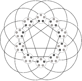
In graph theory, there are different operations that construct a ‘large’ graph from a ‘smaller’ one. Then, the question is what properties of the former can be deduced (or, at least, approximate) from the properties of the latter. One of these operations that recently received some attention in the literature is the construction of token graphs. Namely, from a given graph on vertices and an integer , we construct its token graph on vertices. The name ‘token graph’ comes from an observation in Fabila-Monroy, Flores-Peñaloza, Huemer, Hurtado, Urrutia, and Wood [9], that vertices of correspond to configurations of indistinguishable tokens placed at distinct vertices of , where two configurations are adjacent whenever one configuration can be reached from the other by moving one token along an edge from its current position to an unoccupied vertex. For example, Figure 1 shows the 2-token of the complete graph . The -token graphs are also called symmetric -th power of graphs in Audenaert, Godsil, Royle, and Rudolph [4], and -tuple vertex graphs in Alavi, Lick, and Liu [2]. Token graphs have some applications in physics. For instance, a relationship between token graphs and the exchange of Hamiltonian operators in quantum mechanics is given in Audenaert, Godsil, Royle, and Rudolph [4]. Our interest in the study of token graphs is motivated by some of their applications in mathematics and computer science: Analysis of complex networks, coding theory, combinatorial designs (by means of Johnson graphs), algebraic graph theory, enumerative combinatorics, the study of symmetric functions, etc.
We describe some interesting properties of the Laplacian matrices of and , where is the complement graph of . This leads us to reveal the closed relationship between the algebra of the pair )) with the Bose-Mesner algebra of the Johnson graphs . This paper is structured as follows. In Section 2, we give the preliminaries and background together with some known results. In particular, we introduce the family of Laplacian predistance polynomials, deriving a simple Hoffman-like condition for connectedness. The important family of distance-regular graphs known as Johnson graphs are also introduced as token graphs, together with some of their properties. In Section 3, we first recall some known properties of token graphs’ Laplacian spectra and obtain new related results. Moreover, a result concerning the commutativity of the Laplacian matrices of a graph and its complement was given in [6], but the proof was incomplete, and there were some typos. Here we give the correct proof. Sections 4 and 5 contain the main results of this paper by introducing two new algebras for token graphs, which are closely related to the Bose-Mesner algebra of Johnson graphs. More precisely, in Section 4, for fixed values and graph , the ‘local’ algebra is generated by the pair , and contains the Bose-Mesner algebra . Finally, fixed only , the ‘global’ algebra is generated by some ‘elementary’ adjacency matrices, and contains together with the Laplacian and adjacency matrices of the -token graph of any graph on vertices.
2 Preliminaries and background
In this section, we give the basic notation and definitions. Moreover, together with some known results, we also give some basic new results. Let us start with the formal definition of token graphs.
2.1 Token graphs
Let be a simple graph with vertex set and edge set . By convenience, we consider every edge constituted by two opposite arcs and . Let denote the set of vertices adjacent to , so that the minimum degree of is . For a given integer such that , the -token graph of is the graph whose vertex set consists of the -subsets of vertices of , and two vertices and of are adjacent if and only if their symmetric difference is a pair such that , , and . Then, if has vertices and edges, has vertices and edges. (Indeed, for each edge of , there are edges in .) We also use the notation , with , for a vertex of a 2-token graph. Moreover, we use for the same vertex in the figures. For convenience, we define as a singleton . Moreover, and, by symmetry, . Moreover, if is bipartite, so it is for any .
2.2 Graph spectra and orthogonal polynomials
Given a graph with adjacency matrix and spectrum
where , the predistance polynomials , introduced by Fiol and Garriga in [10], are a sequence of orthogonal polynomials, such that , with respect to the scalar product
| (1) |
normalized in such a way that
Notice that, using this norm, . We can apply the Gram-Schmidt process to to find these polynomials and normalize accordingly. The name given to them is justified because, when is a distance-regular graph, the predistance polynomials become the well-known distance polynomials that applied to yield the distance matrices, that is, .
In a similar way, we can introduce another sequence of orthogonal polynomials from the spectrum of the Laplacian matrix. Let be a graph on vertices, with Laplacian matrix and spectrum
where . The Laplacian predistance polynomials are a sequence of orthogonal polynomials, such that , with respect to the scalar product
| (2) |
normalized in such a way that
As in the previous case, the norm associated with (2) satisfies . In the following proposition, we use the (adjacency and Laplacian) predistance polynomials to give two basic characteristics of graphs, namely, regularity and connectivity. The first assertion is a reformulation of the celebrated Hoffman characterization of regularity, see [14]. The second statement is a Hoffman-type result obtained by using the Laplacian matrix (see, for example, Arsić, Cvetković, Simić, and Škarić [3, p. 19] or Van Dam and Fiol [8, p. 247]).
Proposition 2.1.
Let be a graph with adjacency matrix with distinct eigenvalues and Laplacian matrix with distinct eigenvalues. Let be its predistance polynomials, and its Laplacian predistance polynomials. Consider the sum polynomials and . Let the all- matrix. Then, the following statements hold.
-
[14] is connected and regular if and only if .
2.3 Distance-regular graphs and the Bose-Mesner algebra
Recall that a graph with diameter is distance-regular if, for any pair of vertices , the intersection parameters , , and , for , only depend on the distance , where is the set of vertices adjacent to vertex and is the set of vertices at distance from . Then, we have the intersection array
| (3) |
or quotient matrix
| (9) |
In terms of the predistance polynomials, a characterization of distance-regularity is the following. A graph with diameter and distance matrices
is distance-regular if and only if the predistance polynomials satisfy
| (10) |
In fact, as it was proved in Fiol, Garriga, and Yebra [11], the last equality in (10) involving the highest degree polynomial suffices, namely, .
A way of introducing the Bose-Mesner algebra of a graph is as follows. Let be a graph with diameter , distance matrices , and distinct eigenvalues. Consider the vector spaces
with dimensions and , respectively. Then, is an algebra with the ordinary product of matrices, known as the adjacency algebra of . Moreover, is an algebra with the entry-wise (or Hadamard product) of matrices, defined by , called the distance -algebra of . Notice that, if is regular, then . The most interesting case happens when both algebras coincide.
Theorem 2.2.
Let , , and be as above. Then, is distance-regular if and only if
| (11) |
so that is an algebra with both the ordinary product and the Hadamard product of matrices, and it is known as the Bose-Mesner algebra associated with ,
Since , the equality in (11) is equivalent to
2.4 Johnson graphs
An important class of token graphs are the Johnson graphs (see Fabila-Monroy, Flores-Peñaloza, Huemer, Hurtado, Urrutia, and Wood [9]), that correspond to the -token of the complete graph . In particular , the graph is the octahedron, and is the complement of the Petersen graph , see Figure 1.
In general, the Johnson graph is distance-transitive (and, hence, distance-regular) satisfying the following properties:
-
P1.
The Johnson graph , with , is a distance-regular graph with degree , diameter , and intersection parameters
-
P2.
The Laplacian eigenvalues (and their multiplicities ) of are
For instance, the Laplacian eigenvalues of are and .
-
P3.
Any pair of vertices are at distance , with , if and only if they share elements in common.
-
P4.
The Johnson graph is maximally connected, that is, .
3 On the Laplacian spectra of token graphs
This section deals with some properties of the Laplacian spectra of token graphs. With this aim, let be a graph on vertices. Let and denote the set of -subsets of , which is the set of vertices of the -token graph . For our purpose, it is convenient to denote by the set of all column vectors with entries such that . Let be the eigenvalues of the Laplacian matrix of a graph , with . The second smallest eigenvalue is known as the algebraic connectivity .
Given integers and , the -binomial matrix is an matrix whose rows are the characteristic vectors of the -subsets of in a given order. Thus, if the -th -subset is , then
For instance, for and , we have
By a simple counting argument, one can check that this matrix satisfies
where is the all-1 matrix, see Dalfó, Duque, Fabila-Monroy, Fiol, Huemer, Trujillo-Negrete, and Zaragoza Martínez [6].
The following result enumerate other important properties of the -binomial matrix, proved in the same paper.
Theorem 3.1 ([6]).
Let be a graph with Laplacian matrix . Let be its token graph with Laplacian . Then, the following statements hold:
-
.
-
.
-
The column space (and its orthogonal complement) of is -invariant.
-
The characteristic polynomial of divides the characteristic polynomial of . Thus, .
-
If is a -eigenvector of , then is a -eigenvector of .
-
If is a -eigenvector of such that , then is a -eigenvector of .
Concerning the Laplacian matrices of a graph and its complement, the following result was given in [6], but the proof was incomplete, and there were some typos. So, for completeness, we give here the correct proof.
Proposition 3.2 ([6]).
Let be a graph on vertices, and let be its complement. For a given , the Laplacian matrices of their -token graphs and commute:
Proof.
Let and . We want to prove that for every pair of vertices of and , respectively. To this end, we consider the different possible values of . First, note that when (see after (13) the interpretation of the entry ). Thus, we only need to consider the following three cases:
-
1.
If , that is , we have
(12) -
2.
If , we can assume that and , where and for . Moreover, without loss of generality, we can assume that in implies that in . (If not, interchange the roles of and .) Then, the different terms of the sum
(13) can be seen as ‘walks’ of length two, where the first step is done in , and the second step is done in . When we only have one step, the other corresponds to a loop in the initial or final vertex, represented as or , respectively. Each step gives , except for each loop that provides the vertex degree. We multiply the giving of both steps. This yields the following contributions to the sum:
-
First ‘add ’, and then ‘delete ’:
where , in ; and in . Thus, for each , we get a term .
-
First ‘delete ’, and then ‘add ’:
where , in ; and in . Thus, for each , we get a term .
-
First ‘change by ’, and then ‘keep ’:
where in . This corresponds to the case when and in . Then, since the second step corresponds to the diagonal entry of , this gives the term .
-
The other way around (first ‘keep ’, and then ‘change by ’) corresponds to the case when , but in (since in ). Then, this gives zero.
To summarize, since all the other possibilities give a zero term, we conclude that, when , the total value of the sum in (13) is
(14) With respect to , note that, since the involved matrices are symmetric, we can compute
Reasoning as before, the walks and (from to ) become the walks from to if we interchange these two vertices, the vertices and , and the graphs and . Then, the cases – become:
-
First ‘add ’, and then ‘delete ’:
where , in , and in . Thus, for each , we get again a term .
-
First ‘delete ’, and then ‘add ’:
where , in , and in . Thus, for each , we get a term .
-
First ‘keep ’, and then ‘change by ’:
where in . The first step corresponds to the diagonal entry of , which gives the term again.
-
The other case (first ‘change by ’, and then ‘keep ’) corresponds to , and, since , this gives zero.
Consequently, equals the same expression in (14).
-
-
3.
If , we can assume that and , where and with . Now, the non-zero entries of must correspond to some of the following cases:
-
in and in .
-
in and in .
-
in and in .
-
in and in .
Note and exclude each other, and the same happens with and . Then, at most two of these four cases can be satisfied. Let us assume that we are in some of the cases and (the other cases can be dealt with similarly). Therefore, we get the following situations:
-
First , and then :
-
First , and then :
In each case, we have the term . (Notice that, possibly, both cases hold, and then .)
Similarly, the term can be computed as:
-
First , and then :
-
First , and then :
Thus, in each case, we have again the term .
-
Finally, considering all the cases 1–3, we have that for any and , as claimed. ∎
Here, it is worth mentioning that, in general, this result does NOT hold for the respective adjacency matrices of and .
By a theorem of Frobenius, we get the following consequence.
Corollary 3.3.
The eigenvalues of and can be matched up as in such a way that the eigenvalues of any polynomial in the two matrices is the multiset of the values .
Moreover, since the Laplacian matrix of is , commutes with both and , and every eigenvalue of is the sum of one eigenvalue of and one eigenvalue of . More precisely, we can state the following result about how to pair the eigenvalues.
Proposition 3.4 ([7]).
Let and be the Laplacian matrices of and , respectively. For , let and be the eigenvalues and multiplicities of . Let be the eigenvalues in , with (that is, the non-trivial eigenvalues of ). Let be the eigenvalues in , with . Then,
| (15) |
Part of this result was obtained in Dalfó, Duque, Fabila-Monroy, Fiol, Huemer, Trujillo-Negrete, and Zaragoza Martínez [6], but they did not specify each pair of eigenvalues of and that yields the corresponding eigenvalue of . Later, Dalfó and Fiol addressed this question and established such a pairing in [7, Lemma 2.3], see the following examples.
Example 3.5.
| Spectrum | |||
|---|---|---|---|
| 0 | 0 | 0 | |
| 1 | 3 | 4 | |
| 3 | 1 | 4 | |
| 4 | 0 | 4 | |
| 3 | 3 | 6 | |
| 5 | 1 | 6 |
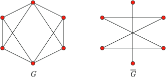
Example 3.6.
Another example is the graph on 6 vertices shown in Figure 3, together with its complement.
| Spectrum | |||
|---|---|---|---|
| 0 | 0 | 0 | |
| 2 | 4 | 6 | |
| 4 | 2 | 6 | |
| 4 | 2 | 6 | |
| 4 | 2 | 6 | |
| 6 | 0 | 6 | |
| 4 | 6 | 10 | |
| 4 | 6 | 10 | |
| 6 | 4 | 10 | |
| 6 | 4 | 10 | |
| 6 | 4 | 10 | |
| 8 | 2 | 10 | |
| 8 | 2 | 10 | |
| 8 | 2 | 10 | |
| 10 | 0 | 10 | |
| 4 | 8 | 12 | |
| 8 | 4 | 12 | |
| 8 | 4 | 12 | |
| 10 | 2 | 12 | |
| 10 | 2 | 12 |
Lemma 3.7.
Let be the -binomial matrix, and let be the distance matrices of the Johnson graph , for . Then,
| (16) |
Proof.
We know that each row of represents a vertex of , as the characteristic vector of the -subset . Then, with the row representing a vertex such that , we have that, from property P3, the vectors and have exactly common 1’s. Thus,
This completes the proof. ∎
Corollary 3.8.
The matrices , , , and commute with each other.
Proof.
Now, we only need to prove that commutes with the other matrices. Since is distance-regular, its distance matrices are polynomials of its adjacency matrix , that is, , and the same holds for because of (16). In particular, is -regular and, hence, its Laplacian matrix can be written as
| (17) |
Solving for , we conclude that can be written as a polynomial of , and, therefore, commutes with . Finally, since both and commute with , so does . ∎
4 A ‘local’ algebra of token graphs
This section introduces a new algebra generated by the Laplacian matrices and , which contains the Bose-Mesner algebra of Johnson graphs.
Let be the -subalgebra of the matrices generated by
the two commuting matrices and . Thus, consists of all -linear combinations of ‘monomials’
where and range from
0 to infinity. Note that and are naturally vector-spaces
over . Moreover, is a subspace of .
Theorem 4.1.
Let and be a graph and its complement on vertices. For some , let and be Laplacian matrices of the token graphs and , respectively. Let be the -vector space of the matrices generated by and . Then, the following statements hold:
-
is a unitary commutative algebra.
-
The Bose-Mesner algebra of the Johnson graph is a subalgebra of .
-
The dimension of is the number, say , of different pairs , for and , defined in Proposition 3.4.
-
If , then there exists a (non-unique) matrix such that
are bases of , where the ’s are the idempotents of .
Proof.
contains the identity matrix , and it is commutative since, by Proposition 3.2,
and commute.
From (17), the adjacency matrix of the Johnson graphs is . Thus, the Bose-Mesner algebra of , generated by , must be a subalgebra of .
This is because, under the hypothesis, we can construct a linear combination of and , say , such that the (symmetric) matrix
has exactly different eigenvalues. Thus, the minimal polynomial of has degree , and every matrix of has a minimal polynomial of degree at most . Thus, the dimension of
is .
This follows directly from .
Notice that, if has different eigenvalues , then its idempotents (orthogonal projections onto the -eigenspaces, see, for instance, Godsil [13, p. 27]) can be written as
∎
From and , notice that
In fact, Gerstenhaber [12], as well as Motzkin and Taussky-Todd [15], proved
independently that the variety of a commuting pair of matrices , is irreducible so that its dimension is also bounded above by the size of the matrices.
The pair generates an algebraic variety (that is, the collection of all common eigenvectors shared by the two matrices).
Example 4.2.
| 0 | 0 | 0 | 0 |
| 1 | 3 | 4 | 5 |
| 3 | 1 | 4 | 7 |
| 4 | 0 | 4 | 8 |
| 3 | 3 | 6 | 9 |
| 5 | 1 | 6 | 11 |
Then, for every matrix , there exists a polynomial such that . In particular .
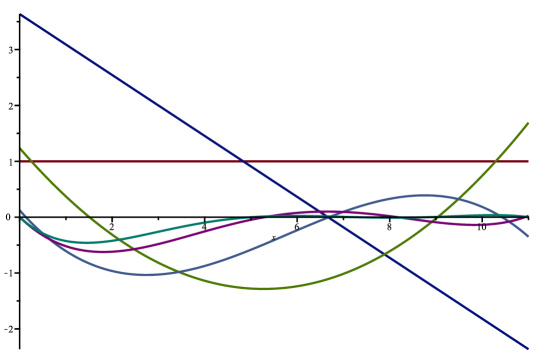
If is 1-regular (all eigenvalues are different), then any matrix that commutes with must be a polynomial in . Described differently, is already in the algebra , that is, . However, is of dimension as is 1-regular, so has dimension . The Laplacian predistance polynomials of are (see Figure 4 for a plot of them):
5 A ‘global’ algebra of token graphs
For given values of and , the ‘local’ algebra of Section 4 is constructed from the Laplacian matrices of the -token graphs of and its complement . In this section, we only fixed and present an algebra containing the Laplacian and adjacency matrices of all the -token graphs of a graph on vertices.
Let be a graph with vertices and edges. Notice that every edge of gives rise to edges in the -token graph . Indeed, we have an edge in every time there is one token moving between and , and the other tokens are in some fixed position in . In particular, each of the edges of , produces edges in the Johnson graph . This suggests the following edge-decomposition of . For every edge of , we consider the graph that consists of the single edge plus the remaining vertices of with no edges between them. Then, we get the following result.
Lemma 5.1.
-
For every edge of , the -token graph consists of independent edges plus isolated vertices.
-
The edges of the Johnson graph are the union of the edges of when runs through all the edges of . So, the edges of the -token graph of a graph are the union of the edges of when runs through all the edges of .
-
The Laplacian [adjacency] matrix [] of is the sum of the Laplacian [adjacency] matrices [] of .
-
Let [] be the Laplacian [adjacency] matrix of a spanning subgraph of . Then is the -token graph of some graph on vertices if and only if [] is the sum of the Laplacian [adjacency] matrices [] of where runs through all edges of :
(18)
Proof.
Here we only need to prove that all the edges of have no vertices in common. If is an edge of , then two any edges of are of the form , , with , , , and , where and . Thus, are different vertices of . – All the statements in these items follow from the following fact: Let be a subgraph of . Then, there exist an edge of if and only if for some edge in (and also in ). Thus, for , if and only if . Moreover, if , all the edges of with endpoint contribute with the value and, hence . The equality for the adjacency matrix is also clear. ∎
In other words, the -token graph of a graph on vertices can be seen as the sum of the -token graphs of some ‘elementary’ graphs . In terms of matrices, the Laplacian or adjacency matrices of are a linear combination, with coefficients and of the ‘elementary’ matrices or , respectively.
In particular, if a Laplacian matrix can be written as a linear combination of the matrices , , then commutes with (since is, in fact the Laplacian matrix of a -token graph, and Corollary 3.8 applies).
Theorem 5.2.
For some fixed and , let be, for , the adjacency matrices of the token graphs . Let be the -vector space of the matrices generated by the matrices . Then, the following statements hold:
-
is a unitary non-commutative algebra.
-
For any graph , the algebra of Theorem 4.1 is a subalgebra of .
-
The dimension of is , with a basis constituted by the matrices , for .
Proof.
It is clear since, if the edges and has a vertex in common, the matrices and do not commute. Using (18), we only need to prove that the Laplacian matrices , for , belong to . As corresponds to a graph with a series of independent vertices, is a diagonal matrix with 1’s in the entries corresponding to the endpoints of such edges. Then, the statement follows from the equality (see Example 5.3). No pair of matrices have a common entry , so that they are linearly independent. ∎
Example 5.3.
In the case of , with vertices , the adjacency and Laplacian matrices, indexed by the vertices of in the order , and induced by the edge are:
Concerning the Laplacian matrices, the following result shows that the algebra of Theorem 4.1 can be constructed only if the condition of commutativity in Proposition 3.2 holds.
Proposition 5.4.
Let and be, respectively, the Laplacian matrices of a spanning subgraph of and its complement with respect to . Then, and commute if and only if and are the -token graphs of some graph , on vertices, and its complement .
Proof.
If and , then we know, by Proposition 3.2, that and commute. To prove the converse, we use Corollary 3.8, by noting that and commute if and only if and do. However, if and do not commute, cannot be written as a -linear combination of some matrices , for (see the last comment after Lemma 5.1). Consequently, by the same lemma, if and do not commute, neither nor can be -token graphs. ∎
References
- [1] Y. Alavi, M. Behzad, P. Erdős, and D. R. Lick, Double vertex graphs, J. Comb. Inf. Syst. Sci. 16 (1991), no. 1, 37–50.
- [2] Y. Alavi, D. R. Lick, and J. Liu, Survey of double vertex graphs, Graphs Combin. 18 (2002) 709–715.
- [3] B. Arsić, D. Cvetković, S. K. Simić, and M. Škarić, Graph spectral techniques in computer sciences, Appl. Anal. Discrete Math. 6 (2012), no. 1, 1–30.
- [4] K. Audenaert, C. Godsil, G. Royle, and T. Rudolph, Symmetric squares of graphs, J. Combin. Theory B 97 (2007) 74–90.
- [5] W. Carballosa, R. Fabila-Monroy, J. Leaños, and L. M. Rivera, Regularity and planarity of token graphs, Discuss. Math. Graph Theory 37 (2017), no. 3, 573–586.
- [6] C. Dalfó, F. Duque, R. Fabila-Monroy, M. A. Fiol, C. Huemer, A. L. Trujillo-Negrete, and F. J. Zaragoza Martínez, On the Laplacian spectra of token graphs, Linear Algebra Appl. 625 (2021) 322–348.
- [7] C. Dalfó and M. A. Fiol, On the algebraic connectivity of token graphs, J. Algebraic Combin., accepted, 2023, https://arxiv.org/abs/2209.01030.
- [8] E. R. van Dam and M. A. Fiol, The Laplacian spectral excess theorem for distance-regular graphs, Linear Algebra Appl. 458 (2014) 245–250.
- [9] R. Fabila-Monroy, D. Flores-Peñaloza, C. Huemer, F. Hurtado, J. Urrutia, and D. R. Wood, Token graphs, Graphs Combin. 28 (2012), no. 3, 365–380.
- [10] M. A. Fiol and E. Garriga, From local adjacency polynomials to locally pseudo distance-regular graphs, J. Combin. Theory Ser. B 7I (1997) 162–183.
- [11] M. A. Fiol, E. Garriga, and J. L. A. Yebra, Locally pseudo-distance-regular graphs, J. Combin. Theory Ser. B 68 (1996) 179–205.
- [12] M. Gerstenhaber, On dominance and varieties of commuting matrices, Ann. of Math. 73 (1961) 324–348.
- [13] C. D. Godsil, Algebraic Combinatorics, Chapman and Hall, New York, 1993.
- [14] A. J. Hoffman, On the polynomial of a graph, Amer. Math. Monthly 70 (1963) 30–36.
- [15] T. Motzkin and O. Taussky-Todd, Pairs of matrices with property L. II, Trans. Amer. Math. Soc. 80 (1955) 387–401.
- [16] V. Nikiforov, The spectral radius of subgraphs of regular graphs, Electron. J. Combin. 14 (2007) #N20.