Gravitational helicity flux density from two-body systems

Jinzhuang Dong, Jiang Long and Run-Ze Yu

School of Physics, Huazhong University of Science and Technology,
Luoyu Road 1037, Wuhan, Hubei 430074, China

The helicity flux density is a novel quantity which characterizes the angular distribution of the helicity of radiative gravitons and it may be tested by gravitational wave experiments in the future. We derive a quadrupole formula for the helicity flux density due to gravitational radiation in the slow motion and the weak field limit. We apply the formula to the bound and unbound orbits in two-body systems and find that the total radiative helicity fluxes are always zero. However, the helicity flux density still has non-trivial dependence on the angle. We also find a formula for the total helicity flux by including all contributions of the higher multipoles.

1 Introduction

Gravitational wave, one of the great predictions of general relativity, has been detected several years ago [1]. It is well known that gravitational waves carry energy, linear momentum as well as angular momentum during their propagation. The energy loss due to gravitational radiation, which is governed by the famous formula [2]

$$\frac{dE}{dud\Omega}=-T(u,\Omega),\quad T(u,\Omega)=\frac{1}{32\pi G}\dot{C}_{AB}\dot{C}^{AB},$$ (1.1)

has been observed indirectly in a pulsar binary system, PSR B1913+16 by Hulse and Taylor 50 years ago [3, 4]. In this formula, the coordinate $u$ is the retarded time and $\Omega=(\theta,\phi)$ are spherical coordinates of the celestial sphere. The shear tensor $C_{AB}$ is symmetric and traceless whose time derivative $\dot{C}_{AB}=\frac{\partial}{\partial u}C_{AB}$ is the news tensor. All the indices are lowered by the metric $\gamma_{AB}$ of the unit sphere and raised by its inverse $\gamma^{AB}$. Recently, a new observable $O(u,\Omega)$, which is called helicity flux density, has been derived in the context of flat holography [5, 6]

$$O(u,\Omega)=\frac{1}{32\pi G}\dot{C}_{AB}C^{B}_{\ C}\epsilon^{CA},$$ (1.2)

where $\epsilon^{AB}$ is the Levi-Civita tensor on the unit sphere. This operator naturally arises from the generalized superrotation [7] and the requirement of the closure of the Lie algebra. The operator is defined at future null infinity $\mathcal{I}^{+}$ and obeys the flux equation

$$\frac{dH}{dud\Omega}=O(u,\Omega),$$ (1.3)

where $H$ is helicity flux across $\mathcal{I}^{+}$. At the microscopic level, the helicity flux evaluates the difference between the numbers of gravitons with left and right helicity. Therefore, the operator $O(u,\Omega)$ characterizes the rate of change of helicity flux in unit time and unit solid angle. In the context of asymptotic symmetry [2, 8, 9], the smeared operator

$$\mathcal{O}_{g}=\int dud\Omega g(\Omega)O(u,\Omega)$$ (1.4)

generates super-duality transformation [5] which rotates the gravitational electric-magnetic duality transformations locally. The super-duality transformation is also called “dual supertranslation” [10, 11, 12] in the literature and contributes to the precession of freely falling gyroscopes [13], an extension of the spin memory effect [14]. Note that the helicity flux density operator is also related to the “dual covariant mass aspect” up to a linear term [15, 16].

The formula is valid near $\mathcal{I}^{+}$ and we should relate it to the source that generates the radiation. At the linear level, assuming the source is far away from the observer, the energy loss is mainly from the variation of the quadrupole [17, 18, 19, 20]. In [21], the energy loss due to gravitational radiation has been discussed for Kepler orbits. The results have been extended to hyperbolic orbits in [22, 23, 24]. The radiation of the linear momentum and the angular momentum have been discussed in [25, 26]. See also recent development in [27, 28, 29, 30]. It is natural to ask for a parallel quadrupole formula for the helicity flux density in gravitational radiation.

This paper is organized as follows. In section 2 we will derive the quadrupole formula for the helicity flux density. In section 3, we will apply the quadrupole formula to various orbits in the two-body systems of astrophysics. We will extend the quadrupole formula by including higher multipoles in the following section and discuss our results in section 5. The details on the integrals on the unit sphere are collected in the Appendix A.

2 The quadrupole formula

In the weak field limit, the metric $g_{\mu\nu}$ around the Minkowski spacetime can be expanded as

$$g_{\mu\nu}=\eta_{\mu\nu}+h_{\mu\nu},$$ (2.1)

where $h_{\mu\nu}$ is the perturbation of the gravitational wave and $\eta_{\mu\nu}$ is the Minkowski matrix. We may define a trace-reversed tensor

$$\bar{h}_{\mu\nu}=h_{\mu\nu}-\frac{1}{2}\eta_{\mu\nu}h$$ (2.2)

with $h=\eta^{\mu\nu}h_{\mu\nu}$ the trace of $h_{\mu\nu}$. At the linear level, by imposing the Lorenz gauge $\partial^{\mu}\bar{h}_{\mu\nu}=0$, the trace-reversed perturbation can be solved by Green’s function and is determined by the stress tensor $T_{\mu\nu}$ of the source [31]

$$\bar{h}_{\mu\nu}=4G\int d^{3}\bm{x}^{\prime}\frac{T_{\mu\nu}(t-|\bm{x}-\bm{x}^{\prime}|,\bm{x}^{\prime})}{|\bm{x}-\bm{x}^{\prime}|}.$$ (2.3)

We assume the source moves slowly and the size $a$ of the source is much smaller than the distance $r=|\bm{x}|$

$$a\ll r.$$ (2.4)

As a consequence, the trace-reversed perturbation is related to the second time derivative of the quadrupole moment

$$\bar{h}_{ij}=\frac{2G}{r}\ddot{I}_{ij}(u),$$ (2.5)

where $I_{ij}$ is the quadrupole momentum tensor

$$I_{ij}(u)=\int d^{3}\bm{x}T_{00}(u,\bm{x})x^{i}x^{j}.$$ (2.6)

The symmetric traceless perturbation $h^{\text{T}}_{ij}=h_{ij}-\frac{1}{3}\delta_{ij}h$ is determined by

$$h^{\text{T}}_{ij}=\frac{2G}{r}\ddot{M}_{ij}(u),$$ (2.7)

where the reduced quadrupole momentum $M_{ij}$ is symmetric and tracelss

$$M_{ij}=I_{ij}-\frac{1}{3}\delta_{ij}I,\quad I=\delta^{kl}I_{kl}.$$ (2.8)

We may project the symmetric traceless perturbation to the symmetric traceless and transverse mode

$$h^{\text{TT}}_{ij}=\left(P_{i}^{k}P_{j}^{l}-\frac{1}{2}P_{ij}P^{kl}\right)h^{\text{T}}_{kl},$$ (2.9)

where

$$P_{ij}=\delta_{ij}-n_{i}n_{j}$$ (2.10)

is the projector and $n_{i}$ is the unit normal vector on the sphere

$$n_{i}=(\sin\theta\cos\phi,\sin\theta\sin\phi,\cos\theta).$$ (2.11)

Therefore, the shear tensor can be read out from the limit

$$C_{AB}=\lim{}_{+}rY^{i}_{A}Y^{j}_{B}h_{ij}^{\text{TT}}=2G(Y^{i}_{A}Y^{j}_{B}+\frac{1}{2}\gamma_{AB}n^{i}n^{j})\ddot{M}_{ij},$$ (2.12)

where $\lim{}_{+}$ is defined by keeping the retarded time $u$ fixed and taking the limit $r\to\infty$. The vectors $Y^{i}_{A},\ i=1,2,3$ are three conformal Killing vectors which are related to the normal vector by

$$Y^{i}_{A}=-\nabla_{A}n_{i}.$$ (2.13)

Their explicit expressions and various relevant identities can be found in [32, 33]. After some efforts, we find the following quadrupole formula for the helicity flux density

$$\frac{dH}{dud\Omega}=\frac{G}{8\pi}\dddot{M}_{ij}\ddot{M}_{kl}Q^{ijkl},$$ (2.14)

where

$$Q^{ijkl}= -\delta^{jk}\epsilon^{ilm}n_{m}+\epsilon^{ilm}n^{j}n^{k}n_{m}-\frac{1}{2}\epsilon^{klm}n^{i}n^{j}n_{m}-\frac{1}{2}\epsilon^{ijm}n^{k}n^{l}n_{m}.$$ (2.15)

Note that the last two terms contribute zero since the Levi-Civita tensor is antisymmetric while the reduced quadrupole is symmetric. Therefore, we may drop them and rewrite $Q^{ijkl}$ as

$$Q^{ijkl}=-\delta^{jk}\epsilon^{ilm}n_{m}+\epsilon^{ilm}n^{j}n^{k}n_{m}=-P^{jk}\epsilon^{ilm}n_{m}.$$ (2.16)

For a periodic system, we may also define the time average of the helicity flux density in a period $T$

$$\langle\frac{dH}{dud\Omega}\rangle=\frac{1}{T}\int_{0}^{T}du\frac{dH}{dud\Omega}=\frac{G}{8\pi}\langle\dddot{M}_{ij}\ddot{M}_{kl}\rangle Q^{ijkl}.$$ (2.17)

As a comparison, we can also reproduce the quadrupole formula for the energy flux density

$$\frac{dE}{dud\Omega}=-\frac{G}{8\pi}\dddot{M}_{ij}\dddot{M}_{kl}E^{ijkl},$$ (2.18)

where

$$E^{ijkl}=\delta^{jl}\delta^{ik}-2\delta^{ik}n^{j}n^{l}+\frac{1}{2}n^{i}n^{j}n^{k}n^{l}.$$ (2.19)

Note that the tensor $Q^{ijkl}$ contains odd numbers of $n_{i}$ in each term. Therefore, the total helicity flux would be zero

$$\frac{dH}{du}=\int d\Omega\frac{dH}{dud\Omega}=0.$$ (2.20)

It seems that there is no non-trivial helicity flux which can be found. However, the point is that the expression (2.14) is local, and it is expected to detect a non-trivial helicity flux distribution on the celestial sphere. In other words, the quantity (1.4) would be non-zero for general function $g$, characterizing the angular dependence of the helicity flux density. The quadrupole formula (2.14) is one of the main results of this paper. Another important quantity is the total helicity flux density during a time interval for generic orbits

$$\frac{dH}{d\Omega}=\int_{t_{\text{in}}}^{t_{\text{out}}}du\frac{dH}{dud\Omega}=\frac{G}{8\pi}\int_{t_{\text{in}}}^{t_{\text{out}}}du\dddot{M}_{ij}\ddot{M}_{kl}Q^{ijkl}.$$ (2.21)

3 Two-body systems

3.1 Setup

We will discuss the two-body system which is firstly studied in [21]. The masses of the two stars are denoted as $M_{1}$ and $M_{2}$ respectively and the labels 1 and 2 are used to distinguish the objects. The orbital trajectories of the two stars are

$$x_{(i)}=x_{(i)}(t),\quad y_{(i)}=y_{(i)}(t),\quad z_{(i)}=0,\quad i=1,2.$$ (3.1)

The action of this two-body system is

$$S=\int dt[\frac{1}{2}M_{1}(\dot{x}_{(1)}^{2}+\dot{y}_{(1)}^{2})+\frac{1}{2}M_{2}(\dot{x}_{(2)}^{2}+\dot{y}_{(2)}^{2})+\frac{GM_{1}M_{2}}{\sqrt{(x_{(1)}-x_{(2)})^{2}+(y_{(1)}-y_{(2)})^{2}}}]$$ (3.2)

and the equations of motion are as follows

$$\ddot{x}_{(1)} = -\frac{GM_{2}(x_{(1)}-x_{(2)})}{\left((x_{(1)}-x_{(2)})^{2}+(y_{(1)}-y_{(2)})^{2}\right)^{3/2}},$$ (3.3)

$$\ddot{y}_{(1)} = -\frac{GM_{2}(y_{(1)}-y_{(2)})}{\left((x_{(1)}-x_{(2)})^{2}+(y_{(1)}-y_{(2)})^{2}\right)^{3/2}},$$ (3.4)

$$\ddot{x}_{(2)} = \frac{GM_{1}(x_{(1)}-x_{(2)})}{\left((x_{(1)}-x_{(2)})^{2}+(y_{(1)}-y_{(2)})^{2}\right)^{3/2}},$$ (3.5)

$$\ddot{y}_{(2)} = \frac{GM_{1}(y_{(1)}-y_{(2)})}{\left((x_{(1)}-x_{(2)})^{2}+(y_{(1)}-y_{(2)})^{2}\right)^{3/2}}.$$ (3.6)

As a consequence, we find

$$M_{1}\ddot{x}_{(1)}+M_{2}\ddot{x}_{(2)}=M_{1}\ddot{y}_{(1)}+M_{2}\ddot{y}_{(2)}=0.$$ (3.7)

The two stars move around their center-of-mass which may be chosen as the origin of the Cartesian coordinate system

$$M_{1}x_{(1)}+M_{2}x_{(2)}=M_{1}y_{(1)}+M_{2}y_{(2)}=0.$$ (3.8)

The distance $D$ of the two stars is

$$D=\sqrt{(x_{(1)}-x_{(2)})^{2}+(y_{(1)}-y_{(2)})^{2}}.$$ (3.9)

Similarly, the distance between star $i$ ($i=1,2$) and the center-of-mass would be

$$D_{i}=\sqrt{x_{(i)}^{2}+y_{(i)}^{2}}.$$ (3.10)

Therefore, the relation among $D_{1},D_{2}$ and $D$ is

$$D_{1}=\frac{M_{2}}{M_{1}+M_{2}}D,\quad D_{2}=\frac{M_{1}}{M_{1}+M_{2}}D,\quad M_{1}D_{1}=M_{2}D_{2}.$$ (3.11)

We may define a new coordinate system

$$x=x_{(1)}-x_{(2)},\quad y=y_{(1)}-y_{(2)},\quad z=z_{(1)}-z_{(2)}$$ (3.12)

and then the action becomes

$$S=\int dt[\frac{1}{2}\frac{M_{1}M_{2}}{M_{1}+M_{2}}(\dot{x}^{2}+\dot{y}^{2})+\frac{GM_{1}M_{2}}{\sqrt{x^{2}+y^{2}}}].$$ (3.13)

Therefore, the motion of the two-body system is equivalent to a test particle with a reduced mass

$$\mu=\frac{M_{1}M_{2}}{M_{1}+M_{2}}$$ (3.14)

moving around a fixed object whose mass is

$$\bar{M}=M_{1}+M_{2}.$$ (3.15)

The Cartesian coordinates $(x,y)$ may be transformed to the polar coordinates $(D,\psi)$ through

$$D=r\cos\psi,\quad y=D\sin\psi.$$ (3.16)

There are several typical orbits which may be parameterized as follows.

1. Circular orbits. The two stars are separated by a constant distance

   $$D=a$$ (3.17)

   and they revolve around each other at a constant angular velocity

   $$\dot{\psi}=\sqrt{\frac{G\bar{M}}{a^{3}}}.$$ (3.18)

   The period of the orbit is

   $$T=\frac{2\pi}{\dot{\psi}}=2\pi\sqrt{\frac{a^{3}}{G\bar{M}}}.$$ (3.19)

2. Elliptic orbits. The semi-major axis and the eccentricity of the ellipse are $a$ and $e$ ($0<e<1$), respectively. Then the elliptic orbit can be parameterized as

   $$D=\frac{\epsilon}{1+e\cos\psi},\quad\epsilon=a(1-e^{2}).$$ (3.20)

   The periastron ($\psi=0$) and apoastron ($\psi=\pi$) distances are

   $$D_{p}=\frac{\epsilon}{1+e}=a(1-e),\quad D_{a}=\frac{\epsilon}{1-e}=a(1+e),$$ (3.21)

   and the time evolutions of $D$ and $\psi$ are respectively

   $$\dot{D}=\sqrt{\frac{G\bar{M}}{\epsilon}}e\sin\psi,\quad\dot{\psi}=\frac{\sqrt{G\bar{M}\epsilon}}{D^{2}}.$$ (3.22)

   The period of the orbit is

   $$T=\int_{0}^{2\pi}\frac{d\psi}{\dot{\psi}}=2\pi\sqrt{\frac{a^{3}}{G\bar{M}}},$$ (3.23)

   which is formally the same as the period of the circular orbits. After some algebra, we find the following conserved energy

   $$\frac{1}{2}\mu\dot{D}^{2}-\frac{G\bar{M}\mu}{D}=-\frac{GM_{1}M_{2}}{2a},$$ (3.24)

   which is indeed negative for any elliptic orbits.

3. Parabolic orbits. The orbital trajectory is represented by

   $$D=\frac{\epsilon}{1+\cos\psi}$$ (3.25)

   with eccentricity $e=1$. The orbit can be obtained from elliptic orbits by taking the limit $e\to 1$ while keeping $\epsilon$ finite. This is an unbound orbit and the periastron distance is

   $$D_{p}=\frac{\epsilon}{2}.$$ (3.26)

   The time evolution of the orbit is the same as (3.22) with $e=1$ and the initial/final angle $\psi_{\text{in}/\text{out}}$ is

   $$\psi_{\text{in}}=-\pi,\quad\psi_{\text{out}}=\pi.$$ (3.27)

4. Hyperbolic orbits. The orbital trajectory may be parameterized by

   $$D=\frac{\epsilon}{1+e\cos\psi},\quad\epsilon=a(e^{2}-1),$$ (3.28)

   where $a$ is the semi-major axis and the eccentricity $e$ is larger than 1 ($e>1$). The semi-major axis $a$ is related to the initial velocity $v_{\text{in}}$

   $$a=\frac{G\bar{M}}{v_{\text{in}}^{2}}$$ (3.29)

   while the eccentricity may be expressed as

   $$e=\sqrt{1+\frac{b^{2}v_{\text{in}}^{4}}{G^{2}\bar{M}^{2}}}$$ (3.30)

   with $b$ the impact parameter. This is an unbound orbit and the initial/final angle $\psi_{\text{in}/\text{out}}$ has been chosen as

   $$\psi_{\text{in}}=-\arccos\left(-\frac{1}{e}\right)\equiv-A,\quad\psi_{\text{out}}=\arccos\left(-\frac{1}{e}\right)\equiv A.$$ (3.31)

   The periastron distance is

   $$D_{p}=\frac{\epsilon}{1+e}=a(e-1)$$ (3.32)

   while the time evolution of the distance $D$ and the angle $\psi$ is still given by (3.22), except that one should replace $\epsilon$ by $\epsilon=a(e^{2}-1)$. Note that the parabolic orbits can also be obtained by taking the limit $e\to 1$ while keeping $\epsilon$ finite from the hyperbolic orbits.

3.2 Circular orbits

As an illustration, we will apply our formula to a binary system where two stars have equal mass $M$. This system can be found in the textbook [31]. The two stars are in a circular orbit in the $x$-$y$ plane and their distance is $D=2R$. The radius $R$ is extremely large such that the inner structure of the two stars can be ignored and we will treat them as two points. In the Newtonian limit, the angular frequency of the circular orbit is

$$\omega=\sqrt{\frac{GM}{4R^{3}}}.$$ (3.33)

The orbits of the two stars are

$$x_{(1)}=R\cos\omega t,\quad y_{(1)}=R\sin\omega t,\quad z_{(1)}=0,$$ (3.34)

$$x_{(2)}=-R\cos\omega t,\quad y_{(2)}=-R\sin\omega t,\quad z_{(2)}=0,$$ (3.35)

and the energy density of the system is

$$T_{00}(t,\bm{x})=M\delta(z)[\delta(x-x_{(1)})\delta(y-y_{(1)})+\delta(x-x_{(2)})\delta(y-y_{(2)})].$$ (3.36)

Therefore, the non-vanishing quadrupole of the binary system is

$$I_{11}=MR^{2}(1+\cos 2\omega u),\quad I_{22}=MR^{2}(1-\cos 2\omega u),\quad I_{12}=MR^{2}\sin 2\omega u.$$ (3.37)

The reduced quadrupole moment becomes

$$M_{11}=\frac{1}{3}MR^{2}(1+3\cos 2\omega u),$$ (3.38)

$$M_{22}=\frac{1}{3}MR^{2}(1-3\cos 2\omega u),$$ (3.39)

$$M_{33}=-\frac{2}{3}MR^{2},$$ (3.40)

$$M_{12}=M_{21}=MR^{2}\sin 2\omega u.$$ (3.41)

By calculating the second and third time derivative of the reduced quadrupole moment and substituting them into (2.17), we find the time average of the helicity flux density

$$\langle\frac{dH}{dud\Omega}\rangle =\frac{GM^{2}R^{4}\omega^{5}(7\cos\theta+\cos 3\theta)}{\pi}$$

$$=\frac{G^{7/2}M^{9/2}(7\cos\theta+\cos 3\theta)}{32\pi R^{7/2}c^{5}},$$ (3.42)

where we have inserted the velocity of light into the formula in the last step. Note that the velocity of the star 1 ( or 2) is

$$v=\sqrt{\frac{GM}{4R}},$$ (3.43)

we may rewrite the average helicity flux density as

$$\langle\frac{dH}{dud\Omega}\rangle=\frac{4}{\pi}Mc^{2}\left(\frac{v}{c}\right)^{7}(7\cos\theta+\cos 3\theta).$$ (3.44)

Obviously, it has the dimension of energy since the dimension of the helicity is the same as the angular momentum. We define the characteristic value

$$E_{c}=\frac{32}{\pi}Mc^{2}\left(\frac{v}{c}\right)^{7}=\frac{G^{7/2}M^{9/2}}{4\pi R^{7/2}c^{5}}$$ (3.45)

to represent the magnitude of the helicity flux density. For the event GW150914 [1], the mass of the two black holes are approximately the same

$$M\approx 30M_{\odot}$$ (3.46)

and their distance is estimated as

$$D=350\text{km}.$$ (3.47)

Therefore, the characteristic magnitude of the helicity flux density is

$$E_{c}\approx 3.5\times 10^{45}\text{kg}\cdot\text{m}^{2}/\text{s}^{2}\approx 3\times 10^{79}\hbar/\text{s}.$$ (3.48)

There is a huge number of gravitons radiated out. However, due to the large distance of the event ($d\approx cz/{H}_{0}\approx 380\text{Mpc}$), the gravitons are diluted when arriving at the earth. Now we will discuss the angular distribution of the helicity flux

$$h(\theta)=\frac{1}{8}(7\cos\theta+\cos 3\theta).$$ (3.49)

Some properties are listed in the following.

1. The helicity flux density is symmetric with respect to the equatorial plane. In other words, it has odd parity under transformation $\theta\to\pi-\theta$

   $$h(\pi-\theta)=-h(\theta).$$ (3.50)

2. Since the function $h(\theta)$ is parity odd, it vanishes at $\theta=\frac{\pi}{2}$

   $$h(\frac{\pi}{2})=0.$$ (3.51)

3. The helicity flux density approaches its maximum value at the north pole ($\theta=0$) and minimum value at the south pole ($\theta=\pi$)

   $$\langle\frac{dH}{dud\Omega}\rangle_{\text{max}}=E_{c},\quad\langle\frac{dH}{dud\Omega}\rangle_{\text{min}}=-E_{c}.$$ (3.52)

4. The function $h(\theta)$ is a monotonic decreasing function

   $$h^{\prime}(\theta)<0,\quad\theta\in(0,\pi).$$ (3.53)

In the figure 1, we plot the angular distribution of the helicity flux. Since the distribution is invariant by the rotation around the $z$ axis, we only draw the $\theta$ dependence in this figure.

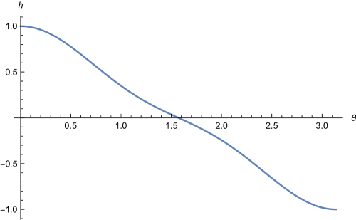
Figure 1: Angular distribution of the helicity flux. The function $h(\theta)$ is abbreviated to $h$.

3.3 Elliptic orbits

The orbital trajectories of star 1 and 2 are given by

$$x_{(1)}=D_{1}\cos\psi,\quad y_{(1)}=D_{1}\sin\psi,\quad z_{(1)}=0,$$ (3.54)

$$x_{(2)}=-D_{2}\cos\psi,\quad y_{(2)}={-}D_{2}\sin\psi,\quad z_{(2)}=0.$$ (3.55)

The energy density of the binary system can be expressed as

$$T_{00}(t,\bm{x})=M_{1}\delta(x-x_{(1)})\delta(y-y_{(1)})\delta(z)+M_{2}\delta(x-x_{(2)})\delta(y-y_{(2)})\delta(z).$$ (3.56)

Correspondingly, the non-vanishing quadrupole components are

$$I_{11}=I\cos^{2}\psi,\quad I_{22}=I\sin^{2}\psi,\quad I_{12}=I_{21}=I\sin\psi\cos\psi,$$ (3.57)

where $I$ is the trace of the quadrupole

$$I=\mu D^{2}.$$ (3.58)

The reduced quadrupole is

$$M_{ij}=I\left(\begin{array}[]{ccc}\cos^{2}\psi-\frac{1}{3}&\sin\psi\cos\psi&0\\ \sin\psi\cos\psi&\sin^{2}\psi-\frac{1}{3}&0\\ 0&0&-\frac{1}{3}\end{array}\right).$$ (3.62)

As a consequence, we find

$$\ddot{M}_{11} = \frac{G\bar{M}\mu}{\epsilon}[-\frac{2e^{2}}{3}+\frac{1}{6}e(-13\cos\psi-3\cos 3\psi)-2\cos 2\psi],$$ (3.63)

$$\ddot{M}_{22} = \frac{G\bar{M}\mu}{\epsilon}[\frac{4e^{2}}{3}+\frac{1}{6}e(17\cos\psi+3\cos 3\psi)+2\cos 2\psi],$$ (3.64)

$$\ddot{M}_{33} = -\frac{G\bar{M}\mu}{\epsilon}\frac{2}{3}e(e+\cos\psi),$$ (3.65)

$$\ddot{M}_{12} = \ddot{M}_{21}=-\frac{G\bar{M}\mu}{\epsilon}\sin\psi[-(e(\cos 2\psi+3)+4\cos\psi)]$$ (3.66)

for the second time derivative of the reduced quadrupole and

$$\dddot{M}_{11} = \frac{(G\bar{M})^{3/2}\mu}{\epsilon^{5/2}}(1+e\cos\psi)^{2}\frac{1}{3}\sin\psi(e(9\cos 2\psi+11)+24\cos\psi),$$ (3.67)

$$\dddot{M}_{22} = -\frac{(G\bar{M})^{3/2}\mu}{\epsilon^{5/2}}(1+e\cos\psi)^{2}\frac{1}{3}\sin\psi(e(9\cos 2\psi+13)+24\cos\psi),$$ (3.68)

$$\dddot{M}_{33} = \frac{(G\bar{M})^{3/2}\mu}{\epsilon^{5/2}}(1+e\cos\psi)^{2}\frac{2}{3}e\sin\psi,$$ (3.69)

$$\dddot{M}_{12} = \dddot{M}_{21}=\frac{(G\bar{M})^{3/2}\mu}{\epsilon^{5/2}}(1+e\cos\psi)^{2}\frac{1}{2}(-5e\cos\psi-3e\cos 3\psi-8\cos 2\psi)$$ (3.70)

for the third time derivative of the reduced quadrupole. We can define a time average quantity

$$G_{ij,kl}=\langle\dddot{M}_{ij}\ddot{M}_{kl}\rangle=\frac{1}{T}\int_{0}^{T}du\dddot{M}_{ij}\ddot{M}_{kl}=\frac{1}{T}\int_{0}^{2\pi}d\psi\dddot{M}_{ij}\ddot{M}_{kl}\dot{\psi}^{-1}=G_{0}g_{ij,kl},$$ (3.71)

where $G_{0}$ is

$$G_{0}=\frac{(G\bar{M})^{5/2}\mu^{2}}{a^{3/2}\epsilon^{2}}$$ (3.72)

and the non-vanishing components of $g_{ij,kl}$ are

$$g_{11,12} = g_{11,21}=\frac{1}{12}\left(-37e^{2}-48\right),$$ (3.73)

$$g_{12,11} = g_{21,11}=\frac{1}{12}\left(37e^{2}+48\right),$$ (3.74)

$$g_{12,22} = g_{21,22}=\frac{1}{12}\left(-47e^{2}-48\right),$$ (3.75)

$$g_{12,33} = g_{21,33}=\frac{5}{6}e^{2},$$ (3.76)

$$g_{22,12} = g_{22,21}=\frac{1}{12}\left(47e^{2}+48\right),$$ (3.77)

$$g_{33,12} = g_{33,21}=-\frac{5}{6}e^{2}.$$ (3.78)

Substituting the results into (2.17), the average helicity flux density is

$$\langle\frac{dH}{dud\Omega}\rangle = \frac{1}{8\pi}\frac{G^{7/2}\bar{M}^{5/2}\mu^{2}}{a^{3/2}\epsilon^{2}}g_{ij,kl}Q^{ij,kl}.$$ (3.79)

More explicitly,

$$\langle\frac{dH}{dud\Omega}\rangle = \frac{1}{4\pi}\frac{G^{7/2}\bar{M}^{5/2}\mu^{2}}{a^{3/2}\epsilon^{2}}[(7\cos\theta+\cos 3\theta)+\frac{1}{4}e^{2}\cos\theta\left(5\sin^{2}\theta\cos 2\phi+7\cos 2\theta+21\right)].$$

The result is consistent with the one in circular orbit studied in previous subsection. As the circular case, we may define the angular distribution of the helicity flux as

$$h(\theta,\phi)=\frac{1}{8}[(7\cos\theta+\cos 3\theta)+\frac{1}{4}e^{2}\cos\theta\left(5\sin^{2}\theta\cos 2\phi+7\cos 2\theta+21\right)].$$ (3.81)

Taking the limit as $e\to 0$, it is the same as the function $h(\theta)$. Therefore, it would be better to focus on the contribution from the eccentricity and define a new function

$$g(\theta,\phi)=\frac{1}{32}\cos\theta\left(5\sin^{2}\theta\cos 2\phi+7\cos 2\theta+21\right)$$ (3.82)

whose properties are shown in the following.

1. Discrete symmetry

   $$g(\pi-\theta,\phi)=-g(\theta,\phi),\quad g(\theta,\pi\pm\phi)=g(\theta,\phi).$$ (3.83)

   Therefore, the function $g(\theta,\phi)$ is still parity odd

   $$g(\pi-\theta,\pi+\phi)=-g(\theta,\phi).$$ (3.84)

2. The rotation symmetry around the $z$ axis is broken and the function $g(\theta,\phi)$ depends on $\phi$ explicitly. It is not hard to show that the maximum value of $g(\theta,\phi)$ locates at

   $$(\theta,\phi)=(0,0)\quad\text{or}\quad(0,\pi)$$ (3.85)

   with

   $$g(0,0)=g(0,\pi)=\frac{7}{8}.$$ (3.86)

   By the parity transformation, we find that the minimum value of $g(\theta,\phi)$ locates at

   $$(\theta,\phi)=(\pi,0)\quad\text{or}\quad(\pi,\pi)$$ (3.87)

   with

   $$g(\pi,0)=g(\pi,\pi)=-\frac{7}{8}.$$ (3.88)

We draw the function $g(\theta,\phi)$ on the sphere in figure 2 where

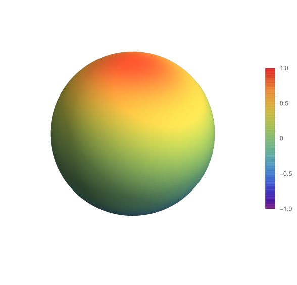
Figure 2: The function $g(\theta,\phi)$ on the sphere. We use different color to represent the value of the function. It is obvious that the red color is distributed in the north pole while the blue color in the south pole.

the angular distribution of the helicity flux is depicted by color in the figure.

We may also draw a contour map in the $\theta$-$\phi$ plane for the function $h(\theta,\phi)$. From figure 3 to figure 5, we have set $e=0.2,0.5,0.9$ respectively and draw the contour map for the function $h(\theta,\phi)$. The dependence of the axis angle $\phi$ becomes more and more important as $e$ increases.

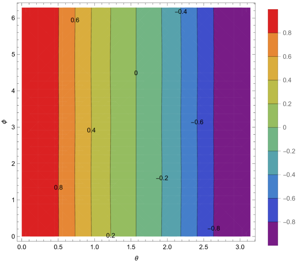
Figure 3: The contour map for the function $h(\theta,\phi)$ for small eccentricity. In this figure, we set $e=0.2$ and the function $h(\theta,\phi)$ is almost independent of $\phi$. The numbers on the contour lines are the values of the function $h(\theta,\phi)$ for the corresponding lines.

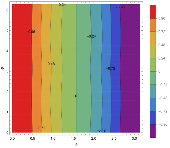
Figure 4: The contour map for the function $h(\theta,\phi)$ for intermediate eccentricity. In this figure, we set $e=0.5$ and the function $h(\theta,\phi)$ depends on $\phi$ weakly. The absolute value of $h(\theta,\phi)$ increases monotonously with increasing eccentricity.

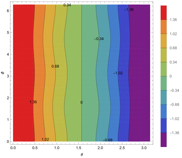
Figure 5: The contour map for the function $h(\theta,\phi)$ for large eccentricity. In this figure, we set $e=0.9$ and the function $h(\theta,\phi)$ is significantly dependent on $\phi$. The absolute value of $h(\theta,\phi)$ still increases monotonously with increasing eccentricity.

3.4 Hyperbolic orbits

We find the same reduced quadrupole (3.62) by replacing $\epsilon$ by $\epsilon=a(e^{2}-1)$. Since the hyperbolic orbit is unbound, we cannot define the time average in a period. However, we can compute the total helicity flux density by

$$\frac{dH}{d\Omega}=\int du\frac{dH}{dud\Omega}=\frac{G}{8\pi}\int_{\psi_{\text{in}}}^{\psi_{\text{out}}}d\psi\dddot{M}_{ij}\ddot{M}_{kl}Q^{ijkl}\dot{\psi}^{-1},$$ (3.89)

where the integrand is

$$\frac{G}{8\pi}\dddot{M}_{ij}\ddot{M}_{kl}Q^{ijkl}\psi^{-1}=\frac{G^{3}\bar{M}^{2}\mu^{2}}{16\pi\epsilon^{2}}g(\theta,\phi;\psi)$$ (3.90)

with

$$g(\theta,\phi;\psi) = (1+e\cos\psi)\cos\theta\times[8(3+\cos 2\theta)$$ (3.91)

$$+e\left(12(\cos 2\theta+3)\cos\psi+2\sin^{2}\theta(3\cos(2\phi-\psi)+\cos(2\phi-3\psi))\right)$$

$$+e^{2}\left((\cos 2\theta+3)(3\cos(2\psi)+1)+2\sin^{2}\theta(3\cos(2(\phi-\psi))+\cos 2\phi)\right)].$$

Therefore, the integral (3.89) is

$$\frac{dH}{d\Omega}=\frac{G^{3}\bar{M}^{2}\mu^{2}}{16\pi\epsilon^{2}}\cos\theta\kappa(\theta,\phi;A)$$ (3.92)

with

$$\kappa(\theta,\phi;A) = 2A\left(5e^{2}\sin^{2}\theta\cos 2\phi+\left(7e^{2}+8\right)\cos 2\theta+21e^{2}+24\right)$$ (3.93)

$$+\frac{1}{3}e\sin A[\sin^{2}\theta\cos 2\phi\left(4\left(3e^{2}+2\right)\cos 2A+63e\cos A+3e\cos 3A+36e^{2}+40\right)$$

$$+6(\cos 2\theta+3)\left(e^{2}\cos 2A+9e\cos A+3e^{2}+20\right)].$$

Still, the total helicity flux is zero while its angular distribution (3.92) is nontrivial. To check the consistency of our result, we continue the result to the elliptic orbits with $0<e<1$. In this case, the integral domain should be $(-\pi,\pi)$ which corresponds to $A=\pi$. Substituting $A=\pi$ into (3.92), we find the following average helicity flux density in a period

$$\langle\frac{dH}{dud\Omega}\rangle = \frac{1}{T}\frac{G^{3}\bar{M}^{2}\mu^{2}}{16\pi\epsilon^{2}}\cos\theta\kappa(\theta,\phi;\pi)$$ (3.94)

$$= \frac{G^{7/2}\bar{M}^{5/2}\mu^{2}}{16\pi a^{3/2}\epsilon^{2}}\cos\theta\left(5e^{2}\sin^{2}\theta\cos 2\phi+\left(7e^{2}+8\right)(\cos 2\theta+3)\right)$$

which is exactly the equation (LABEL:helicityelliptic).

The function $\kappa(\theta,\phi;A)$ may be separated into two parts. The first part depends linearly on $A$

$$\kappa_{1}(\theta,\phi;A)=2A\left(5e^{2}\sin^{2}\theta\cos 2\phi+\left(7e^{2}+8\right)\cos 2\theta+21e^{2}+24\right),$$ (3.95)

while the second part is a superposition of sine and cosine functions of $A$

$$\kappa_{2}(\theta,\phi;A) = \frac{1}{3}e\sin A[\sin^{2}\theta\cos 2\phi\left(4\left(3e^{2}+2\right)\cos 2A+63e\cos A+3e\cos 3A+36e^{2}+40\right)$$ (3.96)

$$+6(\cos 2\theta+3)\left(e^{2}\cos 2A+9e\cos A+3e^{2}+20\right)]$$

$$= \frac{2\sqrt{e^{2}-1}}{3e^{2}}[3\left(2e^{2}+13\right)e^{2}(\cos 2\theta+3)+\left(12e^{4}+e^{2}+2\right)\sin^{2}\theta\cos 2\phi]$$

In the high eccentricity limit, the asymptotic behaviors of $\kappa_{1}$ and $\kappa_{2}$ are

$$\kappa_{1}(\theta,\phi;A) \sim \pi e^{2}\left(5\sin^{2}\theta\cos 2\phi+7\cos 2\theta+21\right),$$ (3.97)

$$\kappa_{2}(\theta,\phi;A) \sim 4e^{3}\left(2\sin^{2}\theta\cos 2\phi+\cos 2\theta+3\right).$$ (3.98)

Therefore, the second part becomes more important than the first part in the high eccentricity limit. On the other hand, taking the limit as $e\to 1$, the second part becomes zero while the first part is still finite. To find the characteristic value of $e$ such that $\kappa_{1}\approx\kappa_{2}$, we notice that both of them reach their maximum values at the north pole

$$\kappa_{1}(0,0;A) = 8\left(7e^{2}+8\right)\arccos\left(-\frac{1}{e}\right),$$ (3.99)

$$\kappa_{2}(0,0;A) = 8\sqrt{e^{2}-1}\left(2e^{2}+13\right).$$ (3.100)

They are equal to each other at

$$e\approx e_{c}=5.3.$$ (3.101)

We separate the hyperbolic orbits into two classes according to the eccentricity, $1<e<e_{c},\ e>e_{c}$. From figure 6 to figure 8, we draw the contour map for the angular distribution of the total helicity flux for $e=1.4,\ 5$ and $10$.

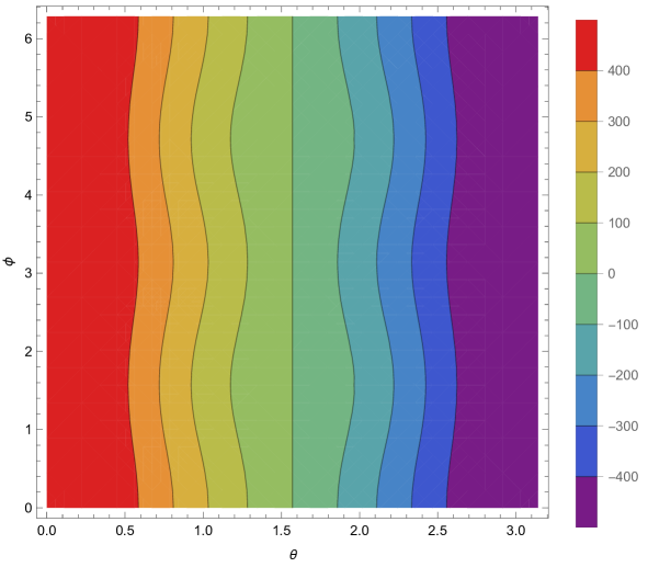
Figure 6: The angular distribution of the total helicity flux in the $\theta$-$\phi$ plane. We have set $e=1.4$ in this figure. The pattern of the contour lines is similar to the one in figure 5, though we have used a different normalization here.

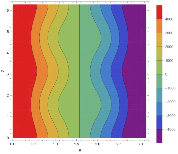
Figure 7: The angular distribution of the total helicity flux in the $\theta$-$\phi$ plane. We have set $e=5$ in this figure. The contour lines are more tortuous than the one in figure 6.

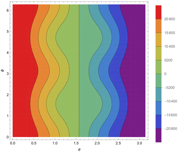
Figure 8: The angular distribution of the total helicity flux in the $\theta$-$\phi$ plane. We have set $e=10$ in this figure. The pattern of the contour lines are almost the same as one in figure 7, except that the absolute value becomes much more larger.

Note that we can also compute the total energy flux density for hyperbolic orbits

$$\frac{dE}{d\Omega}=-\frac{G}{8\pi}\int_{\psi_{\text{in}}}^{\psi_{\text{out}}}d\psi\dddot{M}_{ij}\dddot{M}_{kl}E^{ijkl}\dot{\psi}^{-1},$$ (3.102)

where the integrand is

$$-\frac{G}{8\pi}\dddot{M}_{ij}\dddot{M}_{kl}E^{ijkl}\dot{\psi}^{-1}=-\frac{G^{7/2}\bar{M}^{5/2}\mu^{2}}{512\pi\epsilon^{7/2}}p(\theta,\phi;\psi)$$ (3.103)

with

$$p(\theta,\phi;\psi) = (1+e\cos\psi)^{2}\left(-2\sin^{2}\theta\cos 2(\phi-\psi)+\cos 2\theta+3\right)$$ (3.104)

$$\times[36e^{2}\sin^{2}\theta\sin 4\psi\sin 2\phi+8\left(15e^{2}+32\right)\sin^{2}\theta\sin 2\psi\sin 2\phi+36e^{2}\sin^{2}\theta\cos 4\psi\cos 2\phi$$

$$+2\cos 2\psi\left(4\left(15e^{2}+32\right)\sin^{2}\theta\cos 2\phi+30e^{2}(\cos 2\theta+3)\right)-25e^{2}\cos 2(\theta-\phi)$$

$$-25e^{2}\cos 2(\theta+\phi)+68e^{2}\cos 2\theta+50e^{2}\cos 2\phi+204e^{2}+320e\sin^{2}\theta\sin\psi\sin 2\phi$$

$$+192e\sin^{2}\theta\sin 3\psi\sin 2\phi+192e\sin^{2}\theta\cos 3\psi\cos 2\phi$$

$$+64e\cos\psi\left(5\sin^{2}\theta\cos 2\phi+4\cos 2\theta+12\right)+128\cos 2\theta+384].$$

Therefore, the total energy flux density is

$$\frac{dE}{d\Omega}=-\frac{G^{7/2}\bar{M}^{5/2}\mu^{2}}{512\pi\epsilon^{7/2}}\eta(\theta,\phi;A)$$ (3.105)

with

$$\eta(\theta,\phi;A) = \eta_{1}(\theta,\phi;A)+\eta_{2}(\theta,\phi;A).$$ (3.106)

The first part $\eta_{1}(\theta,\phi;A)$ is proportional to $A$

$$\eta_{1}(\theta,\phi;A) = A[64(28\cos 2\theta+\cos 4\theta+35)+e^{2}\left(208\sin^{2}\theta(\cos 2\theta+3)\cos 2\phi+5416\cos 2\theta+198\cos 4\theta+6802\right)$$ (3.107)

$$+e^{4}\left(-50\sin^{4}\theta\cos 4\phi+32\sin^{2}\theta(\cos 2\theta+3)\cos 2\phi+682\cos 2\theta+\frac{51}{2}\cos 4\theta+\frac{1721}{2}\right)]$$

while the second part is

$$\eta_{2}(\theta,\phi;A) = \frac{\sqrt{e^{2}-1}}{30e^{4}}[704\sin^{4}\theta\cos 4\phi+e^{2}\left(-2912\sin^{4}\theta\cos 4\phi-320\sin^{2}\theta(\cos 2\theta+3)\cos 2\phi\right)$$

$$+e^{4}\left(4712\sin^{4}\theta\cos 4\phi+2080\sin^{2}\theta(\cos 2\theta+3)\cos 2\phi+5(22440\cos 2\theta+806\cos 4\theta+28082)\right)].$$

Unlike the total helicity flux, the total energy flux is non-vanishing

$$\Delta E = \int d\Omega\frac{dE}{d\Omega}$$

$$= -\frac{G^{7/2}\bar{M}^{5/2}\mu^{2}}{45\epsilon^{7/2}}[2\sqrt{e^{2}-1}\left(673e^{2}+602\right)+6\arccos\left(-\frac{1}{e}\right)\left(37e^{4}+292e^{2}+96\right)].$$

The result matches with the one in [23].

3.5 Parabolic orbits

For parabolic orbits, the total helicity flux density can be found by setting $e=1$ while keeping $\epsilon$ finite. Therefore, we find

$$\frac{dH}{d\Omega}=\frac{5G^{3}\bar{M}^{2}\mu^{2}}{8\epsilon^{2}}\cos\theta\left(\sin^{2}\theta\cos 2\phi+3\cos 2\theta+9\right).$$ (3.110)

The maximum value of $\frac{dH}{d\Omega}$ locates at the points

$$(\theta,\phi)=(0,0)\quad\text{or}\quad(0,\pi)$$ (3.111)

with

$$\frac{dH}{d\Omega}\Big{|}_{\text{max}}=\frac{15G^{3}\bar{M}^{2}\mu^{2}}{2\epsilon^{2}}.$$ (3.112)

Correspondingly, the minimum value of $\frac{dH}{d\Omega}$ locates at the points

$$(\theta,\phi)=(\pi,0)\quad\text{or}\quad(\pi,\pi)$$ (3.113)

with

$$\frac{dH}{d\Omega}\Big{|}_{\text{min}}=-\frac{15G^{3}\bar{M}^{2}\mu^{2}}{2\epsilon^{2}}.$$ (3.114)

4 Higher multipoles

In the previous section, we mainly focus on the contribution of the mass quadrupole. In general, there are higher multipoles contributing to the radiative fluxes. Near future null infinity, the symmetric trace free tensor can be expressed as two types of radiative multipole moments [26]

$$h_{ij}^{\text{TT}}=\frac{4G}{r}(P_{i}^{(i^{\prime}}P_{j}^{j^{\prime})}-\frac{1}{2}P_{ij}P^{i^{\prime}j^{\prime}})\sum_{\ell=2}^{\infty}\frac{n^{i(\ell-2)}}{\ell!}\left(U_{i^{\prime}j^{\prime}i(\ell-2)}-\frac{2\ell}{\ell+1}\epsilon_{i^{\prime}pq}n_{p}V_{j^{\prime}qi(\ell-2)}\right)+\mathcal{O}(r^{-2}),$$ (4.1)

where $U_{i(\ell)}$ are mass-type multipole moments and $V_{i(\ell)}$ are current-type multipole moments. Both of them are symmetric trace free and we use the notation $i(\ell)$ to indicate that the $\ell$ indices $i_{1},i_{2},\cdots,i_{\ell}$ are symmetric trace free. The radiative multipole moments are functionals of the source canonical moments $M_{i(\ell)}$ and $S_{i(\ell)}$

$$U_{i(\ell)}=M^{(\ell)}_{i(\ell)}+\mathcal{O}(G),\quad V_{i(\ell)}=S^{(\ell)}_{i(\ell)}+\mathcal{O}(G)$$ (4.2)

with

$$M^{(\ell)}_{i(\ell)}\equiv\frac{d^{\ell}}{du^{\ell}}M_{i(\ell)},\quad S^{(\ell)}_{i(\ell)}\equiv\frac{d^{\ell}}{du^{\ell}}S_{i(\ell)}.$$ (4.3)

The higher order post-Newtonian corrections to the radiative multipole moments are known and we refer the reader to [34]. The shear tensor may be found as

$$C_{AB}=4GP_{AB}^{ij}\sum_{\ell=2}^{\infty}\frac{n^{i(\ell-2)}}{\ell!}\left(U_{iji(\ell-2)}-\frac{2\ell}{\ell+1}\epsilon_{ipq}n_{p}V_{jqi(\ell-2)}\right),$$ (4.4)

where

$$P_{AB}^{ij}=Y^{i^{\prime}}_{A}Y^{j^{\prime}}_{B}(P^{i}_{(i^{\prime}}P^{j}_{j^{\prime})}-\frac{1}{2}P^{ij}P_{i^{\prime}j^{\prime}})=Y_{A}^{(i}Y_{B}^{j)}-\frac{1}{2}\gamma_{AB}P^{ij}.$$ (4.5)

Correspondingly, the helicity flux density is

$$O(u,\Omega)=\frac{1}{32\pi G}\dot{C}_{AB}C^{B}_{\ C}\epsilon^{CA}$$

$$= \frac{G}{2\pi}P^{iji^{\prime}j^{\prime}}\sum_{\ell,\ell^{\prime}=2}^{\infty}\frac{n^{i(\ell-2)}}{\ell!}\frac{n^{i^{\prime}(\ell^{\prime}-2)}}{\ell^{\prime}!}\left(\dot{U}_{iji(\ell-2)}-\frac{2\ell}{\ell+1}\epsilon_{ipq}n_{p}\dot{V}_{jqi(\ell-2)}\right)\left(U_{i^{\prime}j^{\prime}i^{\prime}(\ell^{\prime}-2)}-\frac{2\ell^{\prime}}{\ell^{\prime}+1}\epsilon_{i^{\prime}p^{\prime}q^{\prime}}n_{p^{\prime}}V_{j^{\prime}q^{\prime}i^{\prime}(\ell^{\prime}-2)}\right),$$

where the rank 4 tensor $P^{iji^{\prime}j^{\prime}}$ is

$$P^{iji^{\prime}j^{\prime}}=P^{ij}_{AB}P^{i^{\prime}j^{\prime}B}_{\hskip 19.91684ptC}\epsilon^{CA}=-\frac{1}{4}(\epsilon^{ij^{\prime}m}P^{ji^{\prime}}+\epsilon^{ii^{\prime}m}P^{jj^{\prime}}+\epsilon^{ji^{\prime}m}P^{ij^{\prime}}+\epsilon^{jj^{\prime}m}P^{ii^{\prime}})n_{m}.$$ (4.7)

The angular distribution of the helicity flux is given by the previous formula. As a consequence, we may find the total radiative rate of the helicity flux

$$\frac{dH}{du}=\int d\Omega\frac{dH}{dud\Omega}=\int d\Omega O(u,\Omega)=\frac{G}{2\pi}\sum_{\ell=2}^{\infty}\frac{\ell+2}{(2\ell+1)!!\ell!(\ell-1)}[\dot{U}_{i(\ell)}V_{i(\ell)}-\dot{V}_{i(\ell)}U_{i(\ell)}].$$ (4.8)

We have used the integrals of the product of the symmetric trace free tensors on the unit sphere which can be found in the Appendix A. As a consistency check, we also compute the energy flux density operator

$$T(u,\Omega) = \frac{G}{4\pi}(P^{ii^{\prime}}P^{jj^{\prime}}+P^{ij^{\prime}}P^{ji^{\prime}}-P^{ij}P^{i^{\prime}j^{\prime}})$$

$$\times\sum_{\ell,\ell^{\prime}=2}^{\infty}\frac{n^{i(\ell-2)}}{\ell!}\frac{n^{i^{\prime}(\ell^{\prime}-2)}}{\ell^{\prime}!}\left(\dot{U}_{iji(\ell-2)}-\frac{2\ell}{\ell+1}\epsilon_{ipq}n_{p}\dot{V}_{jqi(\ell-2)}\right)\left(\dot{U}_{i^{\prime}j^{\prime}i^{\prime}(\ell^{\prime}-2)}-\frac{2\ell^{\prime}}{\ell^{\prime}+1}\epsilon_{i^{\prime}p^{\prime}q^{\prime}}n_{p^{\prime}}\dot{V}_{j^{\prime}q^{\prime}i^{\prime}(\ell^{\prime}-2)}\right).$$

Therefore, the total energy flux is

$$\frac{dE}{du} = -\int d\Omega T(u,\Omega)$$ (4.10)

$$= -\frac{G}{4\pi}\sum_{\ell=2}^{\infty}\frac{(\ell+1)(\ell+2)}{(2\ell+1)!!\ell!\ell(\ell-1)}[\dot{U}_{i(\ell)}\dot{U}_{i(\ell)}+\left(\frac{2\ell}{\ell+1}\right)^{2}\dot{V}_{i(\ell)}\dot{V}_{i(\ell)}],$$

which is exactly the one in [34].

5 Discussion

In this work, we have derived the quadrupole formula (2.14) for helicity flux density in gravitational radiation and apply it to the two-body systems in the slow motion and weak field limit. In all case, the total helicity flux on the sphere is zero while its angular distribution is still non-trivial. For elliptical orbits, we compute the average helicity flux density (LABEL:helicityelliptic) in a period. For parabolic or hyperbolic orbits, we also compute the total helicity flux density during the deflection process. We extend the formula to (4.8) by including the higher multipoles. There are various extensions which deserve study in the future.

1. In the framework of post-Newtonian(PN) expansion, the radiative multipole moments can be expressed as functionals of the source canonical moments [34]. The PN computation of the energy, linear momentum and angular momentum fluxes have been explored to higher PN orders [35]. There are various new effects in higher PN orders, including the radiation reaction correction of the orbits [36, 37, 38, 39, 40], hereditary effects [41, 42, 43] and so on [44]. It would be better to include the higher order corrections in (4.2) to improve the PN expansion of the helicity flux density.

2. In electromagnetic theory, there is a similar helicity flux operator in the context of Carrollian holography [45]. There are already some discussion on the physical consequence of this electromagnetic helicity flux in [46]. The method presents here can be extended to the Maxwell field and one may expect a similar dipole formula for the helicity flux.

3. In this work, we have discussed the helicity flux density for the orbits in Newtonian mechanics. However, in general relativity, the timelike orbits in the out event horizon region in a general Kerr background has been classified [47] in the EMRI limit and the orbits are much more richer. It would be interesting to discuss the helicity flux density for each type of orbits.

4. For real astrophysical systems, the compact stars are extended objects which have internal structure that contribute to the radiative gravitational waves. The problem such as two coalescing neutron stars [48], the black-hole-neutron-star collisions[49] and the intermediate mass-ratio coalescences [50] are interesting topics to study since the helicity flux density may also encodes the information of the internal structure of neutron stars.

Acknowledgments. The work of J.L. was supported by NSFC Grant No. 12005069.

Appendix A Integrals on the unit sphere

In this appendix, we will introduce the necessary details on the symmetric trace free Cartesian tensors and their integrals on the unit sphere. The $\ell$-th symmetric trace free Cartesian tensor is defined as

$$n^{j(\ell)}=n^{j_{1}\cdots j_{\ell}}=n^{j_{1}}\cdots n^{j_{\ell}}-\text{traces},$$ (A.1)

where $n^{j}$ is the unit normal vector on the unit sphere. More explicitly [26],

$$n^{j(\ell)}=\sum_{p=0}^{\lfloor\ell/2\rfloor}a(p;\ell)\delta^{(j_{1}j_{2}}\cdots\delta^{j_{2p-1}j_{2p}}n^{j_{2p+1}}\cdots n^{j_{\ell})}$$ (A.2)

with

$$a(p;\ell)=(-1)^{p}\frac{\ell!(2\ell-2p-1)!!}{2^{p}p!(\ell-2p)!(2\ell-1)!!}.$$ (A.3)

Here the round brackets $(\cdots)$ means that the indices inside the brackets are symmetrized with normalization 1. For example,

$$T^{(ij)}=\frac{1}{2}(T^{ij}+T^{ji}).$$ (A.4)

For each fixed $\ell$, there are $2\ell+1$ independent symmetric trace free Cartesian tensors $n^{j(\ell)}$ which are related to the $\ell$-th spherical harmonic function $Y_{\ell,m},m=-\ell,-\ell+1,\cdots,\ell$ by a linear transformation. The properties of the Cartesian tensors $n^{j(\ell)}$ are shown in the following.

1. Parity. The spherical coordinates of the sphere is denoted as

   $$\Omega=(\theta,\phi).$$ (A.5)

   Under the inverse transformation that sends the point $\Omega$ to its antipodal point $\Omega^{P}$,

   $$P:\Omega\to\Omega^{P}=(\pi-\theta,\pi+\phi),$$ (A.6)

   the normal vector $n^{j}(\Omega)$ flips a sign

   $$n^{j}\to-n^{j}.$$ (A.7)

   As a consequence, the Cartesian tensor $n^{j(\ell)}$ is parity even for $\ell$ even and parity odd for $\ell$ odd respectively

   $$P(n^{j(\ell)})=(-1)^{\ell}n^{j(\ell)}.$$ (A.8)

2. Orthogonality. For two Cartesian tensors $n^{i(\ell)}$ and $n^{j(\ell^{\prime})}$, the integral of their products on the unit sphere is

   $$\frac{1}{4\pi}\int d\Omega n^{i(\ell)}n^{j(\ell^{\prime})}=\frac{\ell!}{(2\ell+1)!!}\Delta^{i(\ell),j(\ell)}\delta_{\ell,\ell^{\prime}}.$$ (A.9)

   It vanishes for $\ell\not=\ell^{\prime}$ and $\Delta^{i(\ell),j(\ell)}$ is the so-called isotropic Cartesian tensor [51]. The isotropic Cartesian tensor $\Delta^{i(\ell),j(\ell)}$ is doubly symmetric traceless in the sense that

   $$\Delta^{i_{1}\cdots i_{\ell},j_{1}\cdots j_{\ell}}=\Delta^{(i_{1}\cdots i_{\ell}),j_{1}\cdots j_{\ell}}=\Delta^{i_{1}\cdots i_{\ell},(j_{1}\cdots j_{\ell})},\quad\Delta^{i_{1}\cdots i_{\ell},j_{1}\cdots j_{\ell}}\delta_{i_{1}i_{2}}=\Delta^{i_{1}\cdots i_{\ell},j_{1}\cdots j_{\ell}}\delta_{j_{1}j_{2}}=0.$$ (A.10)

   The explicit form may be found by combining the fundamental integral on the unit sphere [26]

   $$\frac{1}{4\pi}\int d\Omega n^{j_{1}}\cdots n^{j_{\ell}}=\left\{\begin{array}[]{cc}0&\ell\ \text{odd},\\ \frac{1}{\ell+1}\delta_{(j_{1}j_{2}}\cdots\delta_{j_{\ell-1}j_{\ell})}&\ell\ \text{even}\end{array}\right.$$ (A.13)

   and the equation (A.2), the result is [52]

   $$\Delta^{i(\ell),j(\ell)}=\sum_{p,q}a(p,q;\ell)\delta^{(i_{1}i_{2}}\cdots\delta^{i_{2p-1}i_{2p}}X_{p,q}^{i_{2p+1}\cdots i_{\ell}),(j_{2q+1}\cdots j_{\ell}}\delta^{j_{1}j_{2}}\cdots\delta^{j_{2q-1}j_{2q})},$$ (A.14)

   where $X^{i_{1}\cdots i_{\ell},j_{1}\cdots j_{\ell}}_{0,0}$ is the doubly symmetric rank $2\ell$ tensor which is constructed by Kronecker signature

   $$X^{i_{1}\cdots i_{\ell},j_{1}\cdots j_{\ell}}_{0,0}=X^{i_{1}\cdots i_{\ell},j_{1}\cdots j_{\ell}}=\frac{1}{\ell!}\sum_{\pi\in S_{\ell}}\delta^{i_{1}j_{\pi(1)}}\cdots\delta^{i_{\ell}j_{\pi(\ell)}}$$ (A.15)

   with $S_{\ell}$ the group of the permutations of the first $\ell$ natural numbers. Obviously, it is symmetric for the same type of indices

   $$X^{i_{1}\cdots i_{\ell},j_{1}\cdots j_{\ell}}=X^{(i_{1}\cdots i_{\ell}),j_{1}\cdots j_{\ell}}=X^{i_{1}\cdots i_{\ell},(j_{1}\cdots j_{\ell})}.$$ (A.16)

   The tensor $X_{p,q}^{i_{2p+1}\cdots i_{\ell},j_{2q+1}\cdots j_{\ell}}$ is found by taking the traces $p$ and $q$ times for the $i$ and $j$ indices, respectively

   $$X_{p,q}^{i_{2p+1}\cdots i_{\ell},j_{2q+1}\cdots j_{\ell}}=\delta_{i_{1}i_{2}}\cdots\delta_{i_{2p-1}i_{2p}}X^{i_{1}\cdots i_{\ell},j_{1}\cdots j_{\ell}}_{0,0}\delta_{j_{1}j_{2}}\cdots\delta_{j_{2q-1}j_{2q}}.$$ (A.17)

   The coefficient $a(p,q;\ell)$ is the product of $a(p;\ell)$ and $a(q;\ell)$

   $$a(p,q;\ell)=a(p;\ell)a(q;\ell).$$ (A.18)

   By definition, the isotropic Cartesian tensor $\Delta^{i(\ell),j(\ell)}$ is invariant under the exchange of indices $i(\ell)$ and $j(\ell)$

   $$\Delta^{i(\ell),j(\ell)}=\Delta^{j(\ell),i(\ell)},$$ (A.19)

   and it may be regarded as a projector which projects any rank $\ell$ tensor to its symmetric trace free part

   $$A^{i(\ell)}=\Delta^{i(\ell),j_{1}\cdots j_{\ell}}A^{j_{1}\cdots j_{\ell}}.$$ (A.20)

   In particular,

   $$n^{i(\ell)}=\Delta^{i(\ell),i_{1}^{\prime}\cdots i_{\ell}^{\prime}}n^{i_{1}^{\prime}}\cdots n^{i_{\ell}^{\prime}}=\Delta^{i(\ell),i^{\prime}(\ell)}n^{i^{\prime}(\ell)}.$$ (A.21)

3. Completeness relation. For two Cartesian tensors $n^{i(\ell)}$ with different arguments, we have the summation

   $$\frac{1}{4\pi}\sum_{\ell=0}^{\infty}\frac{(2\ell+1)!!}{\ell!}n^{i(\ell)}(\Omega)n^{i(\ell)}(\Omega^{\prime})=\delta(\Omega-\Omega^{\prime}).$$ (A.22)

   To prove this relation, we need the completeness relation of spherical harmonic functions

   $$\sum_{\ell=0}^{\infty}\sum_{m=-\ell}^{\ell}Y_{\ell,m}(\Omega)Y^{*}_{\ell,m}(\Omega^{\prime})=\delta(\Omega-\Omega^{\prime}).$$ (A.23)

   With the addition theorem of the spherical harmonic function

   $$P_{\ell}(\cos\gamma)=\frac{4\pi}{2\ell+1}\sum_{m=-\ell}^{\ell}Y_{\ell,m}(\Omega)Y^{*}_{\ell,m}(\Omega^{\prime}),$$ (A.24)

   we may rewrite the relation (A.23) as

   $$\frac{1}{4\pi}\sum_{\ell=0}^{\infty}(2\ell+1)P_{\ell}(\cos\gamma)=\delta(\Omega-\Omega^{\prime}).$$ (A.25)

   Note that $\gamma$ is the angle between the two normal vectors $\bm{n}=\bm{n}(\Omega)$ and $\bm{n}^{\prime}=\bm{n}(\Omega^{\prime})$

   $$\bm{n}\cdot\bm{n}^{\prime}=\cos\gamma.$$ (A.26)

   The last ingredient is the addition theorem [51] associated with the symmetric trace free tensor $n^{i(\ell)}$

   $$P_{\ell}(\cos\gamma)=\frac{(2\ell-1)!!}{\ell!}n^{i(\ell)}(\Omega)n^{i(\ell)}(\Omega^{\prime}).$$ (A.27)

   Substituting (A.27) into (A.25), we find the completeness relation (A.22) for the symmetric trace free tensors $n^{i(\ell)}$. With the completeness relation, we may expand functions on the unit sphere as

   $$f(\Omega)=f_{i(\ell)}n^{i(\ell)}(\Omega)$$ (A.28)

   where $f_{i(\ell)}$ is symmetric trace free

   $$f_{i(\ell)}=\frac{1}{4\pi}\frac{(2\ell+1)!!}{\ell!}\int d\Omega f(\Omega)n^{i(\ell)}(\Omega).$$ (A.29)

   For spherical harmonic function,

   $$Y_{\ell,m}(\Omega)=\mathscr{Y}^{\ell,m}_{j(\ell)}n^{j(\ell)},$$ (A.30)

   we have

   $$\mathscr{Y}^{\ell,m}_{j(\ell)}=\frac{1}{4\pi}\frac{(2\ell+1)!!}{\ell!}\int d\Omega Y_{\ell,m}(\Omega)n^{j(\ell)}(\Omega).$$ (A.31)

4. Clebsch-Gordan tensors. Similar to the definition of Clebsch-Gordan coefficients, the Clebsch-Gordan tensors are defined by the integral of three symmetric trace free tensors $n^{i(\ell)}$

   $$\Delta^{i(\ell_{1}),j(\ell_{2}),k(\ell_{3})}=\frac{1}{4\pi}\int d\Omega\ n^{i(\ell_{1})}n^{j(\ell_{2})}n^{k(\ell_{3})}.$$ (A.32)

   After some efforts, we find

   $$\Delta^{i(\ell_{1}),j(\ell_{2}),k(\ell_{3})}=m_{h_{1},h_{2},h_{3}}\Delta^{i(h_{2})\bar{i}(h_{3}),i^{\prime}(h_{2})\bar{i}^{\prime}(h_{3})}\Delta^{j(h_{1})\bar{j}(h_{3}),j^{\prime}(h_{1})\bar{i}^{\prime}(h_{3})}\Delta^{k(h_{1})\bar{k}(h_{2}),j^{\prime}(h_{1})i^{\prime}(h_{2})}\Theta_{h_{1}}\Theta_{h_{2}}\Theta_{h_{3}}.$$ (A.33)

   Here the symbol $\Theta_{h}$ is similar to the step function. It equals to 1 for non-negative integers and 0 otherwise

   $$\Theta_{h}=\left\{\begin{array}[]{cc}1&h=0,1,2,\cdots,\\ 0&\text{others}.\end{array}\right.$$ (A.36)

   The value of the coefficient $m_{h_{1},h_{2},h_{3}}$ is

   $$m_{h_{1},h_{2},h_{3}}=\frac{\ell_{1}!\ell_{2}!\ell_{3}!}{h_{1}!h_{2}!h_{3}!(\ell_{1}+\ell_{2}+\ell_{3}+1)!!}.$$ (A.37)

   To prove the formula (A.33), we may use the identity (A.21) and the integral (A.13)

   $$\Delta^{i(\ell_{1}),j(\ell_{2}),k(\ell_{3})} = \frac{1}{4\pi}\Delta^{i(\ell_{1}),i^{\prime}(\ell_{1})}\Delta^{j(\ell_{2}),j^{\prime}(\ell_{2})}\Delta^{k(\ell_{3}),k^{\prime}(\ell_{3})}\int d\Omega n^{i^{\prime}_{1}}\cdots n^{i^{\prime}_{\ell_{1}}}n^{j^{\prime}_{1}}\cdots n^{j^{\prime}_{\ell_{2}}}n^{k^{\prime}_{1}}\cdots n^{k^{\prime}_{\ell_{3}}}$$ (A.38)

   $$= \frac{1}{(\ell_{1}+\ell_{2}+\ell_{3}+1)!!}\Delta^{i(\ell_{1}),i^{\prime}(\ell_{1})}\Delta^{j(\ell_{2}),j^{\prime}(\ell_{2})}\Delta^{k(\ell_{3}),k^{\prime}(\ell_{3})}\delta_{(i_{1}^{\prime}i_{2}^{\prime}}\cdots\delta_{k^{\prime}_{\ell_{3}-1}k^{\prime}_{\ell_{3}})}.$$

   In the second step, we have assumed the summation $\ell_{1}+\ell_{2}+\ell_{3}$ is even. Since $\Delta^{i(\ell_{1}),j(\ell_{2}),k(\ell_{3})}$ is triplely symmetric traceless

   $$\Delta^{i(\ell_{1}),j(\ell_{2}),k(\ell_{3})}=\Delta^{i_{1}\cdots i_{\ell_{1}},j(\ell_{2}),k(\ell_{3})}=\Delta^{i(\ell_{1}),j_{1}\cdots j_{\ell_{2}},k(\ell_{3})}=\Delta^{i(\ell_{1}),j(\ell_{2}),k_{1}\cdots k_{\ell_{3}}},$$ (A.39)

   $$\Delta^{i_{1}i_{2}\cdots i_{\ell_{1}},j(\ell_{2}),k(\ell_{3})}\delta_{i_{1}i_{2}}=\Delta^{i(\ell_{1}),j_{1}\cdots j_{\ell_{2}},k(\ell_{3})}\delta_{j_{1}j_{2}}=\Delta^{i(\ell_{1}),j(\ell_{2}),k_{1}\cdots k_{\ell_{3}}}\delta_{k_{1}k_{2}}=0,$$ (A.40)

   the non-trivial contributions are from the contractions among $(i^{\prime}j^{\prime}),(j^{\prime}k^{\prime})$ or $(k^{\prime}i^{\prime})$ indices. In other words, we may split the indices as

   $$i(\ell_{1})=i(h_{2})\bar{i}(h_{3}),\quad j(\ell_{2})=j(h_{1})\bar{j}(h_{3}),\quad k(\ell_{3})=k(h_{1})\bar{k}(h_{2}).$$ (A.41)

   Then the number of contractions between $i^{\prime}$ and $j^{\prime}$ indices is $h_{3}$, and so on. It follows that

   $$\ell_{1}=h_{2}+h_{3},\quad\ell_{2}=h_{1}+h_{3},\quad\ell_{3}=h_{1}+h_{2}.$$ (A.42)

   The constants $h_{1},h_{2},h_{3}$ are fixed to

   $$h_{1}=\frac{\ell_{2}+\ell_{3}-\ell_{1}}{2},\quad h_{2}=\frac{\ell_{1}+\ell_{3}-\ell_{2}}{2},\quad h_{3}=\frac{\ell_{1}+\ell_{2}-\ell_{3}}{2}.$$ (A.43)

   Therefore,

   $$\Delta^{i(\ell_{1}),j(\ell_{2}),k(\ell_{3})} = \frac{1}{(\ell_{1}+\ell_{2}+\ell_{3}+1)!!}\Delta^{i(h_{2})\bar{i}(h_{3}),i^{\prime}(h_{2})\bar{i}^{\prime}(h_{3})}\Delta^{j(h_{1})\bar{j}(h_{3}),j^{\prime}(h_{1})\bar{j}^{\prime}(h_{3})}\Delta^{k(h_{1})\bar{k}(h_{2}),k^{\prime}(h_{1})\bar{k}(h_{2})}$$

   $$\times C_{\ell_{1}}^{h_{1}}C_{\ell_{2}}^{h_{2}}C_{\ell_{3}}^{h_{3}}h_{1}!h_{2}!h_{3}!\delta^{i_{1}^{\prime}\bar{k}_{1}^{\prime}}\cdots\delta^{i_{h_{2}}^{\prime}\bar{k}_{h_{2}}^{\prime}}\delta^{\bar{i}^{\prime}_{1}\bar{j}_{1}^{\prime}}\cdots\delta^{\bar{i}^{\prime}_{h_{3}}\bar{j}^{\prime}_{h_{3}}}\delta^{j_{1}^{\prime}k_{1}^{\prime}}\cdots\delta^{j^{\prime}_{h_{1}}k^{\prime}_{h_{1}}}\Theta_{h_{1}}\Theta_{h_{2}}\Theta_{h_{3}}$$

   $$= m_{h_{1},h_{2},h_{3}}\Delta^{i(h_{2})\bar{i}(h_{3}),i^{\prime}(h_{2})\bar{i}^{\prime}(h_{3})}\Delta^{j(h_{1})\bar{j}(h_{3}),j^{\prime}(h_{1})\bar{i}^{\prime}(h_{3})}\Delta^{k(h_{1})\bar{k}(h_{2}),j^{\prime}(h_{1})i^{\prime}(h_{2})}\Theta_{h_{1}}\Theta_{h_{2}}\Theta_{h_{3}}.$$

   In the first step, the factor $C_{\ell_{1}}^{h_{1}}C_{\ell_{2}}^{h_{2}}C_{\ell_{3}}^{h_{3}}h_{1}!h_{2}!h_{3}!$ is the number of terms which contribute to the contractions.

In the following, we will use the previous properties to compute several integrals which are relevant to work. We expand the functions $f(\Omega),\ g(\Omega),\ h(\Omega)$ with the symmetric trace free Cartesian tensors

$$f(\Omega)=f_{i(\ell)}n^{i(\ell)},\quad g(\Omega)=g_{i(\ell)}n^{i(\ell)},\quad h(\Omega)=h_{i(\ell)}n^{i(\ell)},$$ (A.45)

and the corresponding integral properties on the unit sphere as follows

1. The product of $f(\Omega)$ and $g(\Omega)$

   $$\frac{1}{4\pi}\int d\Omega f(\Omega)g(\Omega)=\frac{1}{4\pi}\int d\Omega f_{i(\ell)}n^{i(\ell)}g_{j(\ell^{\prime})}n^{j(\ell^{\prime})}=\frac{\ell!}{(2\ell+1)!!}f_{i(\ell)}g_{i(\ell)}.$$ (A.46)

   $$\frac{1}{4\pi}\int d\Omega f(\Omega)g(\Omega)h(\Omega)=\Delta^{i(\ell_{1}),j(\ell_{2}),k(\ell_{3})}f_{i(\ell_{1})}g_{j(\ell_{2})}h_{k(\ell_{3})}$$ (A.47)

   $$= m_{h_{1},h_{2},h_{3}}f_{i(h_{2})\bar{i}(h_{3})}g_{j(h_{1})\bar{j}(h_{3})}h_{k(h_{1})\bar{k}(h_{2})}\Theta_{h_{1}}\Theta_{h_{2}}\Theta_{h_{3}}.$$

   The result is consistent with the one in [27]. See also similar discussions in [53].

In the total helicity flux, the integrand separates into four parts, $\dot{U}U,\dot{U}V,\dot{V}U$ and $\dot{V}V$. We will discuss them term by term.

1. $\dot{U}U$ terms. Their contributions to the total helicity flux are always zero. We will take the integral

   $$I_{1}=\frac{1}{4\pi}\int d\Omega\epsilon^{ij^{\prime}m}\delta^{ji^{\prime}}n_{m}n^{i(\ell-2)}n^{i^{\prime}(\ell^{\prime}-2)}\dot{U}_{iji(\ell-2)}U_{i^{\prime}j^{\prime}i^{\prime}(\ell^{\prime}-2)}$$ (A.48)

   as an example. Note that the integral is actually

   $$I_{1}=\frac{1}{4\pi}\int d\Omega\epsilon^{ij^{\prime}m}n_{m}n^{i(\ell-2)}n^{i^{\prime}(\ell^{\prime}-2)}\dot{U}_{iji(\ell-2)}U_{jj^{\prime}i^{\prime}(\ell^{\prime}-2)}.$$ (A.49)

   After the integrating on the sphere, the index $m$ is either equal to $i^{\prime}_{k},\ k=1,2,\cdots,\ell-2$ or equal to $j_{k},\ k=1,2,\cdots,\ell^{\prime}-2$. However, since the Levi-Civita tensor is antisymmetric and $U_{i(\ell)}$ is symmetric trace free, the result is always zero.

2. $\dot{V}V$ terms. Their contributions to the total helicity flux are also zero. We will take the integral

   $$I_{2}=\frac{1}{4\pi}\int d\Omega\epsilon^{ij^{\prime}m}n^{j}n^{i^{\prime}}n_{m}n^{i(\ell-2)}n^{i^{\prime}(\ell^{\prime}-2)}\epsilon_{ipq}n_{p}\dot{V}_{jqi(\ell-2)}\epsilon_{i^{\prime}p^{\prime}q^{\prime}}n_{p^{\prime}}V_{j^{\prime}q^{\prime}i^{\prime}(\ell^{\prime}-2)}$$ (A.50)

   as an example. The integral is zero due to the antisymmetric property of Levi-Civita tensor

   $$\epsilon_{i^{\prime}p^{\prime}q^{\prime}}n_{i^{\prime}}n_{p^{\prime}}=0.$$ (A.51)

3. $\dot{U}V$ and $\dot{V}U$ terms. We may choose the integral

   $$I_{3}=\frac{1}{4\pi}\int d\Omega\epsilon^{ij^{\prime}m}\delta^{ji^{\prime}}n_{m}n^{i(\ell-2)}n^{i^{\prime}(\ell^{\prime}-2)}\dot{U}_{iji(\ell-2)}\epsilon_{i^{\prime}p^{\prime}q^{\prime}}n_{p^{\prime}}V_{j^{\prime}q^{\prime}i^{\prime}(\ell^{\prime}-2)}$$ (A.52)

   as an example. Due to the identity

   $$\epsilon_{ij^{\prime}m}\epsilon_{i^{\prime}p^{\prime}q^{\prime}}=\delta_{ii^{\prime}}\delta_{j^{\prime}p^{\prime}}\delta_{mq^{\prime}}+\delta_{ip^{\prime}}\delta_{j^{\prime}q^{\prime}}\delta_{mi^{\prime}}+\delta_{iq^{\prime}}\delta_{j^{\prime}i^{\prime}}\delta_{mp^{\prime}}-\delta_{ii^{\prime}}\delta_{j^{\prime}q^{\prime}}\delta_{mp^{\prime}}-\delta_{ip^{\prime}}\delta_{j^{\prime}i^{\prime}}\delta_{mq^{\prime}}-\delta_{iq^{\prime}}\delta_{j^{\prime}p^{\prime}}\delta_{mi^{\prime}},$$ (A.53)

   we may simplify the integral to

   $$I_{3} = \frac{1}{4\pi}\int d\Omega n_{m}n_{p^{\prime}}n^{i(\ell-2)}n^{i^{\prime}(\ell^{\prime}-2)}\dot{U}_{ii^{\prime}i(\ell-2)}V_{j^{\prime}q^{\prime}i^{\prime}(\ell^{\prime}-2)}(\delta_{iq^{\prime}}\delta_{j^{\prime}i^{\prime}}\delta_{mp^{\prime}}-\delta_{ip^{\prime}}\delta_{j^{\prime}i^{\prime}}\delta_{mq^{\prime}}-\delta_{iq^{\prime}}\delta_{j^{\prime}p^{\prime}}\delta_{mi^{\prime}})$$ (A.54)

   $$= (m_{\ell-2}-2m_{\ell-1})\dot{U}_{i(\ell)}V_{i(\ell)},$$

   where

   $$m_{\ell}=\frac{\ell!}{(2\ell+1)!!}.$$ (A.55)

References

- [1] LIGO Scientific, Virgo Collaboration, B. P. Abbott et al., “Observation of Gravitational Waves from a Binary Black Hole Merger,” Phys. Rev. Lett. 116 (2016), no. 6, 061102, 1602.03837.
- [2] H. Bondi, M. G. J. van der Burg, and A. W. K. Metzner, “Gravitational waves in general relativity. 7. Waves from axisymmetric isolated systems,” Proc. Roy. Soc. Lond. A 269 (1962) 21–52.
- [3] R. A. Hulse and J. H. Taylor, “Discovery of a pulsar in a binary system,” Astrophys. J. Lett. 195 (1975) L51–L53.
- [4] J. H. Taylor and J. M. Weisberg, “A new test of general relativity - Gravitational radiation and the binary pulsar PSR 1913+16,” Astrophysical Journal 253 (Feb., 1982) 908–920.
- [5] W.-B. Liu and J. Long, “Symmetry group at future null infinity III: Gravitational theory,” JHEP 10 (2023) 117, 2307.01068.
- [6] W.-B. Liu and J. Long, “Holographic dictionary from bulk reduction,” Phys. Rev. D 109 (2024), no. 6, L061901, 2401.11223.
- [7] M. Campiglia and A. Laddha, “Asymptotic symmetries and subleading soft graviton theorem,” Phys. Rev. D 90 (2014), no. 12, 124028, 1408.2228.
- [8] R. K. Sachs, “Gravitational Waves in General Relativity. VIII. Waves in Asymptotically Flat Space-Time,” Proceedings of the Royal Society of London Series A 270 (Oct., 1962) 103–126.
- [9] G. Barnich and C. Troessaert, “Symmetries of asymptotically flat 4 dimensional spacetimes at null infinity revisited,” Phys. Rev. Lett. 105 (2010) 111103, 0909.2617.
- [10] H. Godazgar, M. Godazgar, and C. N. Pope, “New dual gravitational charges,” Phys. Rev. D 99 (2019), no. 2, 024013, 1812.01641.
- [11] H. Godazgar, M. Godazgar, and C. N. Pope, “Tower of subleading dual BMS charges,” JHEP 03 (2019) 057, 1812.06935.
- [12] H. Godazgar, M. Godazgar, and M. J. Perry, “Asymptotic gravitational charges,” Phys. Rev. Lett. 125 (2020), no. 10, 101301, 2007.01257.
- [13] A. Seraj and B. Oblak, “Precession Caused by Gravitational Waves,” Phys. Rev. Lett. 129 (2022), no. 6, 061101, 2203.16216.
- [14] S. Pasterski, A. Strominger, and A. Zhiboedov, “New Gravitational Memories,” JHEP 12 (2016) 053, 1502.06120.
- [15] L. Freidel and D. Pranzetti, “Gravity from symmetry: duality and impulsive waves,” JHEP 04 (2022) 125, 2109.06342.
- [16] L. Freidel, D. Pranzetti, and A.-M. Raclariu, “Higher spin dynamics in gravity and w1+ celestial symmetries,” Phys. Rev. D 106 (2022), no. 8, 086013, 2112.15573.
- [17] A. Einstein, “Approximative Integration of the Field Equations of Gravitation,” Sitzungsber. K. Preuss. Akad. Wiss. 1 (1916) 688.
- [18] A. Einstein, “On gravitational waves,” Sitzungsber. K. Preuss. Akad. Wiss. 1 (1918) 154.
- [19] L. D. Landau, The classical theory of fields, vol. 2. Butterworth-Heinemann, 1980.
- [20] K. S. Thorne, C. W. Misner, and J. A. Wheeler, Gravitation. Princeton University Press, 2017.
- [21] P. C. Peters and J. Mathews, “Gravitational radiation from point masses in a Keplerian orbit,” Phys. Rev. 131 (1963) 435–439.
- [22] R. O. Hansen, “Post-Newtonian Gravitational Radiation from Point Masses in a Hyperbolic Kepler Orbit,” Phys.Rev.D 5 (Feb., 1972) 1021–1023.
- [23] M. Turner, “Gravitational radiation from point-masses in unbound orbits: Newtonian results.,” The Astrophysical Journal 216 (Sept., 1977) 610–619.
- [24] S. Capozziello, M. De Laurentis, F. De Paolis, G. Ingrosso, and A. Nucita, “Gravitational waves from hyperbolic encounters,” Mod. Phys. Lett. A 23 (2008) 99–107, 0801.0122.
- [25] P. C. Peters, “Gravitational Radiation and the Motion of Two Point Masses,” Physical Review 136 (Nov., 1964) 1224–1232.
- [26] K. S. Thorne, “Multipole Expansions of Gravitational Radiation,” Rev. Mod. Phys. 52 (1980) 299–339.
- [27] G. Compère, R. Oliveri, and A. Seraj, “The Poincaré and BMS flux-balance laws with application to binary systems,” JHEP 10 (2020) 116, 1912.03164.
- [28] L. Blanchet, G. Compère, G. Faye, R. Oliveri, and A. Seraj, “Multipole expansion of gravitational waves: from harmonic to Bondi coordinates,” JHEP 02 (2021) 029, 2011.10000.
- [29] L. Blanchet, G. Compère, G. Faye, R. Oliveri, and A. Seraj, “Multipole expansion of gravitational waves: memory effects and Bondi aspects,” JHEP 07 (2023) 123, 2303.07732.
- [30] S. Siddhant, A. M. Grant, and D. A. Nichols, “Higher memory effects and the post-Newtonian calculation of their gravitational-wave signals,” 2403.13907.
- [31] S. M. Carroll, Spacetime and geometry. Cambridge University Press, 2019.
- [32] W.-B. Liu and J. Long, “Symmetry group at future null infinity: Scalar theory,” Phys. Rev. D 107 (2023), no. 12, 126002, 2210.00516.
- [33] A. Li, W.-B. Liu, J. Long, and R.-Z. Yu, “Quantum flux operators for Carrollian diffeomorphism in general dimensions,” JHEP 11 (2023) 140, 2309.16572.
- [34] L. Blanchet, “Gravitational Radiation from Post-Newtonian Sources and Inspiralling Compact Binaries,” Living Rev. Rel. 17 (2014) 2, 1310.1528.
- [35] D. Bini, T. Damour, and A. Geralico, “Radiated momentum and radiation reaction in gravitational two-body scattering including time-asymmetric effects,” Phys. Rev. D 107 (2023), no. 2, 024012, 2210.07165.
- [36] T. Damour and N. Deruelle, “General relativistic celestial mechanics of binary systems. I. The post-Newtonian motion.,” Annales de L’Institut Henri Poincare Section (A) Physique Theorique 43 (Jan., 1985) 107–132.
- [37] T. Damour and N. Deruelle, “Radiation Reaction and Angular Momentum Loss in Small Angle Gravitational Scattering,” Phys. Lett. A 87 (1981) 81.
- [38] T. Damour and G. Schaefer, “Higher Order Relativistic Periastron Advances and Binary Pulsars,” Nuovo Cim. B 101 (1988) 127.
- [39] G. Schäfer and N. Wex, “Second post-Newtonian motion of compact binaries,” Physics Letters A 174 (Mar., 1993) 196–205.
- [40] R.-M. Memmesheimer, A. Gopakumar, and G. Schaefer, “Third post-Newtonian accurate generalized quasi-Keplerian parametrization for compact binaries in eccentric orbits,” Phys. Rev. D 70 (2004) 104011, gr-qc/0407049.
- [41] L. Blanchet and T. Damour, “Tail Transported Temporal Correlations in the Dynamics of a Gravitating System,” Phys. Rev. D 37 (1988) 1410.
- [42] L. Blanchet and T. Damour, “Hereditary effects in gravitational radiation,” Phys. Rev. D 46 (1992) 4304–4319.
- [43] L. Blanchet and G. Schaefer, “Gravitational wave tails and binary star systems,” Class. Quant. Grav. 10 (1993) 2699–2721.
- [44] L. Blanchet, “Gravitational radiation from post-Newtonian sources and inspiralling compact binaries,” Living Rev. Rel. 9 (2006) 4.
- [45] W.-B. Liu and J. Long, “Symmetry group at future null infinity II: Vector theory,” JHEP 07 (2023) 152, 2304.08347.
- [46] B. Oblak and A. Seraj, “Orientation memory of magnetic dipoles,” Physical Review D 109 (2024), no. 4, 044037.
- [47] G. Compère, Y. Liu, and J. Long, “Classification of radial Kerr geodesic motion,” Phys. Rev. D 105 (2022), no. 2, 024075, 2106.03141.
- [48] J. P. A. Clark and D. M. Eardley, “Evolution of close neutron star binaries.,” Astrophys. J. 215 (July, 1977) 311–322.
- [49] J. M. Lattimer and D. N. Schramm, “Black-hole-neutron-star collisions,” Astrophys. J. Lett. 192 (1974) L145.
- [50] B. Chen, G. Compère, Y. Liu, J. Long, and X. Zhang, “Spin and Quadrupole Couplings for High Spin Equatorial Intermediate Mass-ratio Coalescences,” Class. Quant. Grav. 36 (2019), no. 24, 245011, 1901.05370.
- [51] S. Hess, Tensors for physics. Springer, 2015.
- [52] W.-B. Liu, J. Long, and X.-H. Zhou, “Quantum flux operators in higher spin theories,” 2311.11361.
- [53] G. Faye, L. Blanchet, and B. R. Iyer, “Non-linear multipole interactions and gravitational-wave octupole modes for inspiralling compact binaries to third-and-a-half post-Newtonian order,” Class. Quant. Grav. 32 (2015), no. 4, 045016, 1409.3546.