Phase transition in the EM scheme of an SDE driven by $\alpha$-stable noises with $\alpha\in(0,2]$

Abstract.

We study in this paper the EM scheme for a family of well-posed critical SDEs with the drift $-x\log(1+\left|x\right|)$ and $\alpha$-stable noises. Specifically, we find that when the SDE is driven by a rotationally symmetric $\alpha$-stable processes with $\alpha=2$ (i.e. Brownian motion), the EM scheme is bounded in the $L^{2}$ sense uniformly w.r.t. the time. In contrast, if the SDE is driven by a rotationally symmetric $\alpha$-stable process with $\alpha\in(0,2)$, all the $\beta$-th moments, with $\beta\in(0,\alpha)$, of the EM scheme blow up. This demonstrates a phase transition phenomenon as $\alpha\uparrow 2$. We verify our results by simulations.

1. Introduction

The following stochastic differential equation (SDE) on $\mathbb{R}^{d}$ has been extensively studied for several decades:

(1.1) $$\,\mathrm{d}X_{t}=f(X_{t})\,\mathrm{d}t+g(X_{t})\,\mathrm{d}L_{t}\ ,\quad X_{0}=x_{0},$$

where $x_{0}\in\mathbb{R}^{d}$, $f:\mathbb{R}^{d}\to\mathbb{R}^{d},g:\mathbb{R}^{d}\to\mathbb{R}^{d\times d}$ satisfy certain regularity conditions, and the process $(L_{t},t\geqslant 0)$ is a $d$-dimensional, rotationally invariant $\alpha$-stable Lévy process with $\alpha\in(0,2]$. We refer to the books [1, 36, 38] for systematic accounts on SDEs driven by Lévy processes and to [2, 3, 5, 6, 7, 8, 16, 17, 19, 20, 30, 10, 18, 40] for more recent developments.

The Euler-Maruyama (EM) scheme of SDE (1.1) has also been studied by many authors, see [29, 30, 22, 41, 13, 42, 14, 39, 32, 4, 33]. In particular, when $f$ is Lipschitz and $g$ is bounded Lipschitz, by a standard method for proving the existence and uniqueness of SDE’s strong solution, it can be shown that the EM scheme in a finite time interval $[0,T]$ strongly converges to (1.1), see for instance [26, 35, 1, 38, 36].

It is well known that, even though a (stochastic) dynamics system is well posed, its numerical schemes may blow up, see [29, 30, 24, 23, 8]. In particular, for SDE (1.1) with a Brownian motion noise, i.e., $\alpha=2$, if the drift coefficient $f$ is a polynomial like $-x|x|^{\theta}$ with $\theta>0$, it has a unique strong solution with finite exponential moment. In contrast, its EM scheme has a blowing-up $L^{p}(\mathbb{P})$ norm with $p\geqslant 1$ as the step size $\eta\rightarrow 0$, see for instance [24, 23, 25]. When the driven noise is an $\alpha$-stable process with $\alpha\in(0,2)$, due to the heavy tailed property of stable distribution, one may expect that the corresponding EM scheme will blow up. One of the main motivation of the present paper is to verify this conjecture.

In this paper, we shall mainly consider SDE (1.1) with a special non-Lipschitz drift $-x\log(1+|x|)$, which lies at the boundary between the cases $-x|x|^{\theta}$ and $-x$. To the best of our knowledge, the behavior of the EM scheme has not been studied. Our main results, Theorems 1.1–1.3, show that the EM scheme is uniformly bounded for $\alpha=2$, but blows up for $\alpha\in(0,2)$. This demonstrates a phase transition as $\alpha\uparrow 2$.

1.1. The drift $-x\log(1+|x|)$ and $\alpha\in(0,2]$: phase transition

In order to demonstrate our idea, we assume for simplicity that $g(x)=I_{d}$ with $I_{d}$ being $d\times d$ identity matrix. We expect that our results can be extended to the case in which $g$ is bounded Lipschitz and nondegenerate.

Let us consider the following SDE on $\mathbb{R}^{d}$:

(1.2) $$\,\mathrm{d}X_{t}=-X_{t}\log(1+\left|X_{t}\right|)\,\mathrm{d}t+\,\mathrm{d}L_{t}\ ,\quad X_{0}=x_{0},$$

where $L_{t}$ is a $d$-dimensional rotationally symmetric $\alpha$-stable Lévy process with $\alpha\in(0,2]$. Thanks to the dissipation of the drift term, we can show by a standard method that SDE (1.2) admits a unique strong solution, see Appendix 6 below.

The Euler-Maruyama (EM) scheme of SDE (1.2) is give by: for $k\in\mathbb{Z}_{+}$,

(1.3) $$Y_{k+1}=Y_{k}-\eta Y_{k}\log(1+\left|Y_{k}\right|)+(L_{(k+1)\eta}-L_{k\eta}),\quad Y_{0}=x_{0},$$

where $\eta>0$ is the step size. We shall show that for $\alpha\in(0,2)$, the above EM scheme $({Y_{n}},n\geq 1)$ blows up in $L^{\beta}(\mathbb{P})$ for any $\beta\in(0,2)$ as $\eta\rightarrow 0$; while for $\alpha=2$, i.e. $L_{t}$ is a standard $d$-dimensional Brownian motion, $({Y_{n}},n\geq 1)$ is uniformly bounded in $L^{2}(\mathbb{P})$. This demonstrates a phase transition as $\alpha\uparrow 2$.

We start with the following theorem for the case of $\alpha=2$.

Theorem 1.1.

Consider the EM scheme (1.3) with $\alpha=2$, i.e. the driven noise is Brownian motion. Then, for any fixed initial value $x_{0}$, there exist constants $\eta_{0}\leqslant\min\{(1+\left|x_{0}\right|)^{-2},\mathrm{e}^{-5}\}$ and $C>0$ such that for all $\eta\in(0,\eta_{0}]$,

(1.4) $$\sup_{m\geqslant 0}\mathbb{E}\left|Y_{m}\right|^{2}\leqslant C.$$

Next we consider the case $\alpha\in(0,2)$, in which $(L_{t},t\geqslant 0)$ is a rotationally symmetric $\alpha$-stable process, which will be denoted by $(Z_{t},t\geqslant 0)$. We refer to [37] for comprehensive account on Lévy processes, stable and more generally, infinitely divisible distributions. See also [16, 31, 28] for more recent developments.

It is known (cf. e.g., [37, Theorem 14.3] or [10, 27]) that the Lévy measure $\nu$ of the process $(Z_{t},t\geqslant 0)$ is

$$\nu(\,\mathrm{d}z)=\frac{C_{d,\alpha}}{\left|z\right|^{d+\alpha}}\,\mathrm{d}z,$$

where constant $C_{d,\alpha}$ is given by

(1.5) $$C_{d,\alpha}=\alpha 2^{\alpha-1}\pi^{-\frac{d}{2}}\cdot\frac{\Gamma\big{(}({d+\alpha})/{2}\big{)}}{\Gamma\big{(}1-{\alpha}/{2}\big{)}}.$$

Even though, for a general $\alpha\in(0,2)$, the transition density function $p_{\alpha}(t,x)$ of the $\alpha$-stable processes $(Z_{t},t\geqslant 0)$ does not have an explicit expression, many of its analytic or asymptotic properties have been known. In particular, it follows from [9, Theorem 2.1] that $p_{\alpha}(t,x)$ satisfies

(1.6) $$K(d,\alpha)^{-1}\frac{t}{(t^{1/\alpha}+\left|x\right|)^{d+\alpha}}\leqslant p_{\alpha}(t,x)\leqslant K(d,\alpha)\frac{t}{(t^{1/\alpha}+\left|x\right|)^{d+\alpha}},\quad x\in\mathbb{R},$$

where $K(d,\alpha)\geqslant 1$ is a constant depending on $d$ and $\alpha$.

By the Lévy-Itô decomposition (cf. [37, Chapter 4] or [1, Chapter 2]), there exists a Poisson random measure $P(\,\mathrm{d}t,\,\mathrm{d}z)$ such that

$$\,\mathrm{d}Z_{t}=\int_{\{\left|z\right|\geqslant 1\}}zP(\,\mathrm{d}t,\,\mathrm{d}z)+\int_{\{\left|z\right|<1\}}z\widetilde{P}(\,\mathrm{d}t,\,\mathrm{d}z),$$

where $\widetilde{P}(\,\mathrm{d}t,\,\mathrm{d}z)=P(\,\mathrm{d}t,\,\mathrm{d}z)-\,\mathrm{d}t\ \nu(\,\mathrm{d}z)$ is the compensated Poisson random measure. Due to the lack of explicit representation for the probability density of the $\alpha$-stable noise $Z_{(n+1)\eta}-Z_{n\eta}$, the numerical simulation becomes complicated and computationally expensive. Hence, one often does not use the scheme (1.3) directly in practice, see [34, 12] for further discussions. Since the $\alpha$-stable distribution and the Pareto distribution with parameter $\alpha$ have the same tail behavior and the stable central limit theorem (see, e.g. [15, 21]), we can replace the stable noise $Z_{(n+1)\eta}-Z_{n\eta}$ with i.i.d. random variables with the Pareto distribution. More precisely, for any fixed time $T>0$, the EM approximation for the SDE (1.2), denoted by mappings $\widetilde{Y}_{k}:\Omega\to\mathbb{R}^{d}$, is given by

(1.7) $$\widetilde{Y}_{k+1}=\widetilde{Y}_{k}-\eta\widetilde{Y}_{k}\log\left(1+\big{|}\widetilde{Y}_{k}\big{|}\right)+\frac{1}{\sigma}\eta^{1/\alpha}\widetilde{Z}_{k+1},\quad\widetilde{Y}_{0}:=x_{0},$$

for all $k\in\left\{0,1,\ldots,n-1\right\}$, $n\in\mathbb{N}$, where $\sigma^{\alpha}=\alpha/(s_{d-1}C_{d,\alpha})$ with $C_{d,\alpha}$ defined by (1.5), $\{\widetilde{Z}_{k},k=1,2,\dotsc\}$ is a sequence of i.i.d. Pareto-distributed random variables, and the density function $p(z)$ of the Pareto distribution is given by

(1.8) $$p(z)=\frac{\alpha}{s_{d-1}|z|^{\alpha+d}}\mathbbm{1}_{(1,\infty)}(|z|).$$

Here, $s_{d-1}=2\pi^{\frac{d}{2}}/\Gamma(\frac{d}{2})$ represents the surface area of the unit sphere $\mathbb{S}^{d-1}\subseteq\mathbb{R}^{d}$.

The following theorem describes the limiting behavior of the EM schemes (1.3) and (1.7) when $\alpha\in(0,2)$. In Theorems 1.2 and 1.3, $\kappa_{\alpha}$ and $\delta_{\alpha}$ are the constants, depending on $\alpha$, given in Lemmas 2.2 and 2.3 below.

Theorem 1.2.

Let $\alpha\in(0,2)$, $\beta\in(0,\alpha)$, $T\in(0,\infty)$ be constants and let $\eta=\frac{T}{n}$ be the step size.

$(\mathrm{i})$ For the EM scheme (1.3), define $K_{1}=2(\mathrm{e}^{\delta_{\alpha}/\beta}+2)/T$. We assume that $T$ and $n$ are large enough such that

$$\frac{T}{n}\leqslant 1,\quad K_{1}<\frac{\delta_{\alpha}-\log\delta_{\alpha}}{\alpha-\beta},\quad\mathrm{e}^{nK_{1}}\geqslant\left|x_{0}\right|\big{(}1+\log(1+\left|x_{0}\right|)\big{)}.$$

Then, there exist a constant $C>0$ and a sequence of non-empty events $\Omega_{n}\subseteq\Omega$, $n\in\mathbb{N}$ with

$$\mathbb{P}(\Omega_{n})\geqslant\frac{C\mathrm{e}^{-\alpha nK_{1}}}{n\delta_{\alpha}^{n}}\quad\text{and}\quad\left|Y_{n}(\omega)\right|\geqslant\exp\left\{nK_{1}+(n-1)\frac{\delta_{\alpha}}{\beta}\right\}$$

for all $\omega\in\Omega_{n}$ and all $n\in\mathbb{N}$ large enough. Consequently, we have

$$\lim_{n\to\infty}\mathbb{E}\left|Y_{n}\right|^{\beta}=\infty.$$

$(\mathrm{ii})$ For the EM scheme (1.7), define $K_{2}=2(\mathrm{e}^{\kappa_{\alpha}/\beta}+2/\sigma)/T$. We assume that $T$ and $n$ are large enough such that

$$\frac{T}{n}\leqslant 1,\quad K_{2}<\frac{\kappa_{\alpha}-\log\kappa_{\alpha}}{\alpha-\beta},\quad\mathrm{e}^{nK_{2}}\geqslant\left|x_{0}\right|\big{(}1+\log(1+\left|x_{0}\right|)\big{)}.$$

Then, there exist a constant $C>0$ and a sequence of non-empty events $\widetilde{\Omega}_{n}\subseteq\Omega$, $n\in\mathbb{N}$ with

$$\mathbb{P}(\widetilde{\Omega}_{n})\geqslant\frac{C\mathrm{e}^{-\alpha nK_{2}}}{n\kappa_{\alpha}^{n}}\quad\text{and}\quad\big{|}{\widetilde{Y}_{n}(\omega)}\big{|}\geqslant\exp\left\{nK_{2}+(n-1)\frac{\kappa_{\alpha}}{\beta}\right\}$$

for all $\omega\in\widetilde{\Omega}_{n}$ and all $n\in\mathbb{N}$ large enough. Consequently, we have

$$\lim_{n\to\infty}\mathbb{E}\big{|}{\widetilde{Y}_{n}}\big{|}^{\beta}=\infty.$$

1.2. The polynomial growth drift and $\alpha\in(0,2)$: blow up

By the same method for showing Theorem 1.2, we can also prove that the EM scheme of SDE (1.1) blows up if the drift has a $p$-order polynomial growth with $p>1$. More precisely, we assume that $f(x)$ and $g(x)$ in SDE (1.1) satisfy the following condition: There exist constants $\gamma>\lambda>1$ and $H\geqslant 1$ such that

(A) $$\max\{\left|f(x)\right|,\left|g(x)\right|\}\geqslant\frac{1}{H}\left|x\right|^{\gamma},\text{ and },\min\{\left|f(x)\right|,\left|g(x)\right|\}\leqslant H\left|x\right|^{\lambda}$$

for all $\left|x\right|\geqslant H$.

Assumption (A) is similar to the condition in [24, Theorem 1]. The EM scheme of the corresponding SDE is

(1.9) $${Y}_{k+1}={Y}_{k}+\eta f\big{(}{Y}_{k}\big{)}+g\big{(}{Y}_{k}\big{)}(Z_{(k+1)\eta}-Z_{k\eta}),\quad{Y}_{0}=x_{0},$$

with step size $\eta=\frac{T}{n}$ and $k\in\{0,1,\dotsc,n-1\}$. In practice, it is easier to consider the following EM scheme:

(1.10) $$\widetilde{Y}_{k+1}=\widetilde{Y}_{k}+\eta f\big{(}\widetilde{Y}_{k}\big{)}+\frac{1}{\sigma}\eta^{1/\alpha}g\big{(}\widetilde{Y}_{k}\big{)}\widetilde{Z}_{k+1},\quad\widetilde{Y}_{0}=x_{0},$$

where $\{\widetilde{Z}_{k},k=1,2,\dotsc\}$ are i.i.d. Pareto distributed random variables.

The following theorem shows that for any $T>0$, both EM schemes (1.9) and (1.10) blow up as $\eta\rightarrow 0$.

Theorem 1.3.

Consider SDE (1.1) under the assumption that $L_{t}$ is a standard $d$-dimensional rotationally invariant $\alpha$-stable process with $\alpha\in(0,2)$. We assume that (A) holds and $g(x_{0})\neq 0$. Let $T>0$ be an arbitrary number and $\eta=\frac{T}{n}$. Then, there exists a constant $c>1$ such that

$(\mathrm{i})$ for the standard EM scheme (1.9), there exists a sequence of non-empty events $\Omega_{n}\subseteq\Omega$, $n\in\mathbb{N}$ such that $\mathbb{P}(\Omega_{n})\geqslant cn^{-c}\delta_{\alpha}^{-n}$. Furthermore, $\left|Y_{n}(\omega)\right|\geqslant 2^{\lambda^{n-1}}$ for all $\omega\in\Omega_{n}$ and all $n\in\mathbb{N}$;

$(\mathrm{ii})$ for the EM scheme (1.10), there exists a sequence of non-empty events $\widetilde{\Omega}_{n}\subseteq\Omega$, $n\in\mathbb{N}$ such that $\mathbb{P}(\widetilde{\Omega}_{n})\geqslant cn^{-c}\kappa_{\alpha}^{-n}$. Furthermore, $\big{|}{\widetilde{Y}_{n}(\omega)}\big{|}\geqslant 2^{\lambda^{n-1}}$ for all $\omega\in\widetilde{\Omega}_{n}$ and all $n\in\mathbb{N}$.

Consequently, for any $\beta\in(0,\alpha)$, we have

$$\lim_{n\to\infty}\mathbb{E}\left|Y_{n}\right|^{\beta}=\infty,\ \text{ and },\ \lim_{n\to\infty}\mathbb{E}\big{|}{\widetilde{Y}_{n}}\big{|}^{\beta}=\infty.$$

The structure of this paper is outlined as follows: We introduce some useful auxiliary lemmas in the following section. In Section 3, we will prove Theorem 1.1. The proofs of Theorems 1.2 and 1.3 are presented in Section 4. In Section 5, we provide numerical simulations that illustrate the convergence and divergence of EM schemes for $d=1$. Finally, in Appendix 6, we establish the existence and uniqueness of the strong solution of SDE (1.2).

2. Preliminary and Auxiliary Lemmas

To prove Theorem 1.1, we will make use of the following lemmas. Since the proof of Lemma 2.1 is elementary, it is omitted.

Lemma 2.1.

If $N$ follows a standard Gaussian distribution, then for any constants $b\geqslant a\geqslant 0$, there exists a constant $C$ such that

(2.1) $$\mathbb{P}(a\leqslant\left|N\right|\leqslant b)\leqslant C(b-a)\mathrm{e}^{-\frac{a^{2}}{2}}.$$

As for the Pareto distribution with parameter $\alpha\in(0,2)$, we have the following lemma.

Lemma 2.2.

Suppose that random vector $\widetilde{Z}:\Omega\to\mathbb{R}^{d}$ satisfies Pareto distribution, then for all $z\in(1,\infty)$ we have

(2.2) $$\mathbb{P}(|\widetilde{Z}|\geqslant z)=\frac{1}{z^{\alpha}}$$

and there exists a constant $\kappa_{\alpha}\geqslant 1$ such that

(2.3) $$\mathbb{P}(z\leqslant|\widetilde{Z}|\leqslant 2z)=\frac{1}{\kappa_{\alpha}z^{\alpha}},$$

where constant $\kappa_{\alpha}=2^{\alpha}/(2^{\alpha}-1)$ which only depends on $\alpha$.

Proof of Lemma 2.2.

For all $z\in(1,\infty)$, and $\alpha\in(0,2)$, we have

$$\mathbb{P}(|\widetilde{Z}|\geqslant z)=\int_{z}^{\infty}\frac{\alpha r^{d-1}}{r^{\alpha+d}}\mathrm{d}r\int_{\mathbb{S}^{d-1}}\frac{1}{s_{d-1}}\mathrm{d}S=\frac{1}{z^{\alpha}}.$$

Similarly, we have

$$\mathbb{P}(z\leqslant|\widetilde{Z}|\leqslant 2z)=\left(1-\frac{1}{2^{\alpha}}\right)\frac{1}{z^{\alpha}}.$$

Taking $\kappa_{\alpha}=2^{\alpha}/(2^{\alpha}-1)$ gives (2.3). ∎

In addition, thanks to inequality (1.6), we also have the following lemma.

Lemma 2.3.

Let $Z:\Omega\to\mathbb{R}^{d}$ be a standard $d$-dimensional rotationally invariant $\alpha$-stable distribution with $\alpha\in(0,2)$. Then for all $z\in(1,\infty)$, we have

(2.4) $$\mathbb{P}(\left|Z\right|\geqslant z)\geqslant\frac{s_{d-1}}{2^{d+\alpha}K(d,\alpha)}\cdot\frac{1}{z^{\alpha}},$$

and there exists a constant $\delta_{\alpha}\geqslant 1$ depending on $d$ and $\alpha$ such that for all $z\in(1,\infty)$,

(2.5) $$\mathbb{P}(z\leqslant\left|Z\right|\leqslant 2z)\geqslant\frac{1}{\delta_{\alpha}z^{\alpha}}.$$

where $\delta_{\alpha}=\frac{2^{d+\alpha}\alpha K(d,\alpha)}{s_{d-1}}\left(1-\frac{1}{2^{\alpha}}\right)^{-1}$ with $s_{d-1}=2\pi^{\frac{d}{2}}/\Gamma(\frac{d}{2})$, and $K(d,\alpha)$ is in (1.6).

Proof.

2.3 The proof is analogous to that of Lemma 2.2. For all $z\in(1,\infty)$, by applying inequality (1.6), we obtain

$$\begin{split}\mathbb{P}(\left|Z\right|\geqslant z)&\geqslant\frac{1}{K(d,\alpha)}\int_{\left|x\right|\geqslant{z}}\!\!\frac{\,\mathrm{d}x}{(1+\left|x\right|)^{d+\alpha}}\\ &\geqslant\frac{s_{d-1}}{2^{d+\alpha}K(d,\alpha)}\int_{z}^{\infty}\!\!\frac{\,\mathrm{d}r}{r^{\alpha+1}}=\frac{s_{d-1}}{2^{d+\alpha}\alpha K(d,\alpha)}\cdot\frac{1}{z^{\alpha}},\end{split}$$

where the second inequality is due to $\left|x\right|\geqslant z>1$. Similarly,

$$\mathbb{P}(z\leqslant\left|Z\right|\leqslant 2z)\geqslant\frac{s_{d-1}}{2^{d+\alpha}\alpha K(d,\alpha)}\left(1-\frac{1}{2^{\alpha}}\right)\cdot\frac{1}{z^{\alpha}}=\frac{1}{\delta_{\alpha}z^{\alpha}}.$$

We complete the proof. ∎

3. EM scheme in the case of $\alpha=2$

In this section, we prove Theorem 1.1. It is easy to see that the EM scheme of (1.2) can be written as

(3.1) $$Y_{k+1}=Y_{k}-Y_{k}\log(1+\left|Y_{k}\right|)\eta+\sqrt{\eta}{N_{k+1}},\quad Y_{0}=x_{0},\quad k=0,1,2,\dotsc,$$

where $\{N_{k},k\geqslant 1\}$ represents a sequence of i.i.d. standard Gaussian random variables and, for each $k\geq 0$, $N_{k+1}$ is independent of $(Y_{j},j\leqslant k)$.

Proof of Theorem 1.1.

Let $n\in\mathbb{N}$ be arbitrary. Denote

$$A_{0}=\Big{\{}\omega\in\Omega:\ \sup_{1\leqslant m\leqslant n}\left|N_{m}(\omega)\right|\in\left[0,\left|\log\eta\right|^{2}\right)\Big{\}}.$$

We make the following claim, whose proof will be postponed.

(3.2) $$\sup_{1\leqslant m\leqslant n}\left|Y_{m}(\omega)\right|\leqslant\eta^{-1/2}\left|\log\eta\right|^{2},\ \ \ \ \omega\in A_{0},$$

and, for all $p\geqslant 2$, there exists a constant $C_{p}$ such that

(3.3) $$\mathbb{E}\left[\sup_{1\leqslant m\leqslant n}|Y_{m}|^{p}\mathbbm{1}_{A^{c}_{0}}\right]\leqslant C_{p}.$$

Let us prove (1.4) first. It follows from (3.2) and (3.3) that

(3.4) $$\begin{split}&\mathrel{\phantom{=}}\mathbb{E}\left[\left|Y_{m}\right|^{2}\log^{2}\big{(}1+\left|Y_{m}\right|\big{)}\right]\\ &=\mathbb{E}\left[\left|Y_{m}\right|^{2}\log^{2}\big{(}1+\left|Y_{m}\right|\big{)}\mathbbm{1}_{A_{0}}\right]+\mathbb{E}\left[\left|Y_{m}\right|^{2}\log^{2}\big{(}1+\left|Y_{m}\right|\big{)}\mathbbm{1}_{A^{c}_{0}}\right]\\ &\leqslant\log^{2}\big{(}1+\eta^{-1/2}\left|\log\eta\right|^{2}\big{)}\mathbb{E}\left|Y_{m}\right|^{2}+C\\ &\leqslant 4|\log\eta|^{2}\mathbb{E}\left|Y_{m}\right|^{2}+C,\end{split}$$

where $C$ can be taken as $C_{p}$ in (3.3) with $p=3$, and the last inequality is by $1+\eta^{-1/2}\left|\log\eta\right|^{2}\leqslant\eta^{-2}$ for $\eta\leqslant\frac{1}{4}$. On the other hand,

(3.5) $$\begin{split}\mathbb{E}\big{[}|Y_{m}|^{2}\log(1+|Y_{m}|)\big{]}&\geqslant\mathbb{E}\big{[}|Y_{m}|^{2}\log(1+|Y_{m}|)\mathbbm{1}_{\{|Y_{m}|\geqslant 2\}}\big{]}\\ &\geqslant\mathbb{E}\big{[}|Y_{m}|^{2}\mathbbm{1}_{\{|Y_{m}|\geqslant 2\}}]\\ &\geqslant\mathbb{E}|Y_{m}|^{2}-4.\end{split}$$

By (3.1), (3.4) and (3.5), we see that for all $0\leqslant m<n$ and $\eta\leqslant\mathrm{e}^{-5}$,

$$\mathbb{E}\left|Y_{m+1}\right|^{2} =\mathbb{E}\left|Y_{m}\right|^{2}-2\eta\mathbb{E}\left[\left|Y_{m}\right|^{2}\log(1+|Y_{m}|)\right]+d\eta+\eta^{2}\mathbb{E}\left[\left|Y_{m}\right|^{2}\log^{2}\big{(}1+\left|Y_{m}\right|\big{)}\right]$$

$$\leqslant\mathbb{E}\left|Y_{m}\right|^{2}-2\eta\mathbb{E}\left[\left|Y_{m}\right|^{2}\right]+(d+8)\eta+\eta^{2}\left[4\left|\log\eta\right|^{2}\mathbb{E}\left|Y_{m}\right|^{2}+C\right]$$

$$\leqslant\big{[}1-2\eta+4\eta^{2}\left|\log\eta\right|^{2}\big{]}\mathbb{E}\left|Y_{m}\right|^{2}+C\eta$$

$$\leqslant\mathrm{e}^{-\eta}\mathbb{E}\left|Y_{m}\right|^{2}+C\eta$$

$$\leqslant\mathrm{e}^{-(m+1)\eta}\left|x_{0}\right|^{2}+C\sum_{k=1}^{m+1}\eta\mathrm{e}^{(k-(m+1))\eta}$$

$$\leqslant\left|x_{0}\right|^{2}+C\mathrm{e}^{-(m+1)\eta}\int_{0}^{(m+1)\eta}\mathrm{e}^{x}\,\mathrm{d}x\leqslant\left|x_{0}\right|^{2}+C.$$

Since $n\in\mathbb{N}$ is arbitrary, (1.4) in Theorem 1.1 clearly holds true.

It remains to show (3.2) and (3.3). For proving (3.2), let $m_{0}=\min\{1\leqslant m\leqslant n:\left|Y_{m}\right|>\eta^{-1/2}\left|\log\eta\right|^{2}\}$ and consider

(3.6) $$Y_{m_{0}}=Y_{m_{0}-1}\big{(}1-\eta\log(1+\left|Y_{m_{0}-1}\right|)\big{)}+\sqrt{\eta}N_{m_{0}}.$$

It is easy to check that as $\eta\leqslant\mathrm{e}^{-5}$

$$\eta\log\big{(}1+\eta^{-1/2}\left|\log\eta\right|^{2}\big{)}\leqslant 1.$$

Since $\left|x_{0}\right|\leqslant\eta^{-\frac{1}{2}}$, (3.2) holds for $m=0$. If $2\left|Y_{m_{0}-1}\right|\leqslant\eta^{-1/2}\left|\log\eta\right|^{2}$, then it follows from (3.6) that for every $\omega\in A_{0}$,

$$\left|Y_{m_{0}}\right|\leqslant\frac{1}{2}\eta^{-1/2}\left|\log\eta\right|^{2}+\sqrt{\eta}\left|\log\eta\right|^{2}\leqslant\eta^{-1/2}\left|\log\eta\right|^{2}.$$

If $2\left|Y_{m_{0}-1}\right|>\eta^{-1/2}\big{(}\left|\log\eta\right|^{2}\big{)}$, due the definition of $m_{0}$, we have

$$\left|Y_{m_{0}}\right| \leqslant\left|Y_{m_{0}-1}\right|\big{(}1-\eta\log(1+{\left|Y_{m_{0}-1}\right|})\big{)}+\sqrt{\eta}\left|N_{m_{0}}\right|$$

$$\leqslant\eta^{-1/2}\left|\log\eta\right|^{2}\Big{[}1-\eta\log\big{(}1+\eta^{-1/2}\left|\log\eta\right|^{2}/2\big{)}\Big{]}+\sqrt{\eta}\left|\log\eta\right|^{2}$$

$$\leqslant\eta^{-1/2}\left|\log\eta\right|^{2}.$$

The last inequality follows from $\eta^{-1/2}\left|\log\eta\right|^{2}\geqslant 2\mathrm{e}$ for all $\eta\leqslant\mathrm{e}^{-2}$. Hence, $m_{0}$ doesn’t exist and claim (3.2) holds.

In order to prove (3.3), we split $A^{c}_{0}$ into the following disjoint events:

$$A_{1} =\Big{\{}\omega\in\Omega:\ \sup_{1\leqslant m\leqslant n}\left|N_{m}(\omega)\right|\in\left[\left|\log\eta\right|^{2},\eta^{-1}\right)\Big{\}};$$

$$A_{k} =\Big{\{}\omega\in\Omega:\ \sup_{1\leqslant m\leqslant n}\left|N_{m}(\omega)\right|\in\left[({k-1}){\eta^{-1}},{k}{\eta^{-1}}\right)\Big{\}},\quad 2\leqslant k\leqslant\lceil\mathrm{e}^{\frac{1}{2\eta}}\rceil=:k_{0};$$

$$B_{k} =\Big{\{}\omega\in\Omega:\ \sup_{1\leqslant m\leqslant n}\left|N_{m}(\omega)\right|\in\left[{k}{\eta^{-1}}\mathrm{e}^{\frac{1}{2\eta}},({k+1}){\eta^{-1}}\mathrm{e}^{\frac{1}{2\eta}}\right)\Big{\}},\quad 1\leqslant k<\infty.$$

Firstly, under $\left|Y_{0}\right|=\left|x_{0}\right|\leqslant{\eta}^{-\frac{1}{2}}$, we verify that for every $1\leqslant k\leqslant\lceil\mathrm{e}^{\frac{1}{2\eta}}\rceil$,

(3.7) $$\sup_{1\leqslant m\leqslant n}\left|Y_{m}(\omega)\right|\leqslant\frac{k}{\eta^{3/2}}\ ,\quad\omega\in A_{k}.$$

Even though this is similar to the proof of (3.2), we still give the detail here for completeness. Notice that $\eta\log\big{(}1+k/(2\eta)\big{)}<\eta\log\big{(}1+(\mathrm{e}^{\frac{1}{2\eta}}+1)/(2\eta)\big{)}<1$. Let $m_{0}=\min\{1\leqslant m\leqslant n:\left|Y_{m}\right|>(k+1)/\eta\}$. If $2\left|Y_{m_{0}-1}\right|\leqslant k\eta^{-\frac{3}{2}}$, then, due to $\eta\leqslant\mathrm{e}^{-5}\leqslant\frac{1}{2}$,

$$\left|Y_{m_{0}}\right|\leqslant\left|Y_{m_{0}-1}\right|+\sqrt{\eta}\left|N_{m_{0}}\right|\leqslant\frac{k}{2\eta^{3/2}}+\frac{k}{\sqrt{\eta}}\leqslant\frac{k}{\eta^{3/2}}.$$

On the other hand, if $2\left|Y_{m_{0}-1}\right|>k\eta^{-\frac{3}{2}}$, then

$$\left|Y_{m_{0}}\right| \leqslant\left|Y_{m_{0}-1}\right|\big{(}1-\eta\log(1+k/(2\eta^{3/2}))\big{)}+\sqrt{\eta}\left|N_{m_{0}}\right|$$

$$\leqslant\frac{k}{\eta^{3/2}}(1-\eta)+\frac{k}{\sqrt{\eta}}\leqslant\frac{k}{\eta^{3/2}},$$

where the second inequality comes from the definition of $m_{0}$ and $\eta\leqslant 2^{-2/3}$. Hence, $m_{0}$ doesn’t exist and the claim (3.7) holds. Besides, Lemma 2.1 yields that

$$\mathbb{P}(A_{1}) \leqslant C\left(\frac{1}{\eta}-\left|\log\eta\right|^{2}\right)\mathrm{e}^{-\left|\log\eta\right|^{2}/2}\leqslant{C}\eta^{\frac{\left|\log\eta\right|}{2}-1},$$

$$\mathbb{P}(A_{k}) \leqslant Cn\cdot\frac{1}{\eta}\mathrm{e}^{-\frac{(k-1)^{2}}{2\eta^{2}}}\leqslant\frac{C}{\eta^{2}}\mathrm{e}^{-\frac{(k-1)^{2}}{2\eta^{2}}},\quad\forall\ 2\leqslant k\leqslant\lceil\mathrm{e}^{\frac{1}{2\eta}}\rceil.$$

It follows that for any $p\geqslant 1$, there is some positive constant $C_{p}^{\prime}$ not depending on $\eta$ such that

(3.8) $$\sum_{k=1}^{k_{0}}\mathbb{E}\left[\sup_{0\leqslant m\leqslant n}\left|Y_{m}\right|^{p}\mathbbm{1}_{A_{k}}\right] \leqslant\frac{C}{\eta^{3p/2}}\cdot\eta^{\frac{\left|\log\eta\right|}{2}-1}+\frac{C}{\eta^{2}}\sum_{k=2}^{\infty}\frac{k^{p}}{\eta^{3p/2}}\mathrm{e}^{-\frac{(k-1)^{2}}{2\eta^{2}}}$$

$$\leqslant C+2^{p}C\sum_{k=1}^{\infty}\left(\frac{k}{\eta}\right)^{\frac{3p}{2}+2}\mathrm{e}^{-\frac{1}{2}\left(\frac{k}{\eta}\right)^{2}}$$

$$\leqslant C+2^{p}C\int_{\lfloor\frac{1}{\eta}\rfloor-1}^{\infty}y^{\frac{3p}{2}+2}\mathrm{e}^{-\frac{y^{2}}{2}}\,\mathrm{d}y\leqslant C_{p}^{\prime},$$

Here the second inequality holds since one can find $\eta\leqslant\mathrm{e}^{-(3p+2)}$ such that $\frac{\left|\log n\right|}{2}-\frac{3p+2}{2}\geqslant 0$ and the fact $(k+1)^{p}\leqslant(2k)^{p}$ for any $k\geqslant 1$ and any fixed $p\geqslant 1$. Besides, $\int_{z}^{\infty}z^{q}\mathrm{e}^{-z^{2}/2}\,\mathrm{d}z<\infty$ for any $q,z>0$ yields the last inequality.

On the event $B_{k}$, due to EM scheme (3.1) and $\left|Y_{0}\right|=\left|x_{0}\right|<\eta^{-\frac{1}{2}}$, we have

$$\left|Y_{1}\right|\leqslant\left|Y_{0}\right|(1+\eta\log(1+\left|Y_{0}\right|))+\sqrt{\eta}\left|N_{1}\right|\leqslant\frac{2(k+1)}{\sqrt{\eta}}\mathrm{e}^{\frac{1}{2\eta}},$$

where the last inequality comes from $\eta^{-\frac{1}{2}}+\sqrt{\eta}\log(1+\eta^{-\frac{1}{2}})\leqslant\eta^{-\frac{1}{2}}\mathrm{e}^{\frac{1}{2\eta}}$ as $\eta\leqslant\frac{1}{2}$. Furthermore, for $\left|Y_{2}\right|$ we have

$$\left|Y_{2}\right| \leqslant\left|Y_{1}\right|(1+\eta\log(1+\left|Y_{1}\right|))+\sqrt{\eta}\left|N_{2}\right|$$

$$\leqslant\frac{2(k+1)}{\sqrt{\eta}}(1+k)\mathrm{e}^{\frac{1}{2\eta}}+\frac{(k+1)}{\sqrt{\eta}}\mathrm{e}^{\frac{1}{2\eta}}$$

$$\leqslant\left[2(k+1)^{2}+(k+1)\right]\frac{1}{\sqrt{\eta}}\mathrm{e}^{\frac{1}{2\eta}}$$

Hence, by induction, we obtain that for each $k\geqslant 1$,

(3.9) $$\left|Y_{m}\right|\leqslant\left[2(k+1)^{m}+(k+1)^{m-1}+\cdots+(k+1)\right]\frac{1}{\sqrt{\eta}}\mathrm{e}^{\frac{1}{2\eta}}:=a_{m}\frac{1}{\sqrt{\eta}}\mathrm{e}^{\frac{1}{2\eta}}.$$

Hence, due to $a_{m}\leqslant 2m(k+1)^{m}$ and $\eta=O(\frac{1}{n})$, we have

$$\sup_{1\leqslant m\leqslant n}\left|Y_{m}\right|\leqslant\frac{2C}{\eta^{3/2}}(k+1)^{\frac{T}{\eta}}\mathrm{e}^{\frac{1}{2\eta}}.$$

Besides, applying Lemma 2.1 again,

$$\mathbb{P}(B_{k})\leqslant\frac{C}{\eta}\mathrm{e}^{-\frac{1}{2}\left(\frac{k}{\eta}\mathrm{e}^{1/(2\eta)}\right)^{2}},\quad\forall\ k\geqslant 1.$$

Due to similar argument (3.8) for any $p\geqslant 1$, there exists a constant $C_{p}^{\prime\prime}$ not depending on $\eta$ such that

(3.10) $$\sum_{k=1}^{\infty}\mathbb{E}\left[\sup_{0\leqslant m\leqslant n}\!\left|Y_{m}\right|^{p}\mathbbm{1}_{B_{k}}\right]\!\!\leqslant\!\frac{2^{p}C^{p+1}}{\eta^{(3p+2)/2}}\sum_{k=1}^{\infty}{(k+1)^{\frac{pC}{\eta}}}\mathrm{e}^{\frac{p}{2\eta}}\cdot\mathrm{e}^{-\frac{1}{2}\left(\frac{k}{\eta}\mathrm{e}^{1/(2\eta)}\right)^{2}}\leqslant\!C_{p}^{\prime\prime}.$$

In sum, equations (3.8) and (3.10)yield that there exists a constant $C_{p}$ not depending on $\eta$ such that

$$\mathbb{E}\left[\sup_{1\leqslant m\leqslant n}|Y_{m}|^{p}\mathbbm{1}_{A^{c}_{0}}\right]\leqslant\sum_{k=1}^{k_{0}}\mathbb{E}\left[\sup_{0\leqslant m\leqslant n}\!\left|Y_{m}\right|^{p}\mathbbm{1}_{A_{k}}\right]+\sum_{k=1}^{\infty}\mathbb{E}\left[\sup_{0\leqslant m\leqslant n}\!\left|Y_{m}\right|^{p}\mathbbm{1}_{B_{k}}\right]\leqslant C_{p}\ ,$$

that is, (3.3) holds. And we complete the proof. ∎

4. EM scheme in the case of $\alpha\in(0,2)$

In this section, we prove Theorems 1.2 and 1.3.

Proof of Theorem 1.2.

We only prove Part $(\mathrm{ii})$ of the theorem in detail, since Part $(\mathrm{i})$ can be shown in a similar way by replacing the estimates in Lemma 2.2 with the ones in Lemma 2.3.

Recall the formulations of (1.7):

$$\widetilde{Y}_{k+1}=\widetilde{Y}_{k}-\eta\widetilde{Y}_{k}\log\left(1+\big{|}\widetilde{Y}_{k}\big{|}\right)+\frac{1}{\sigma}\eta^{1/\alpha}\widetilde{Z}_{k+1},\quad\widetilde{Y}_{0}:=x_{0},$$

where $\eta=\frac{T}{n}$ for all $k=,0,1,\dotsc,n-1$, and the definition of $K_{2}$ in the theorem:

$$K_{2}=\frac{2}{T}\left(\mathrm{e}^{\kappa_{\alpha}/\beta}+\frac{2}{\sigma}\right),$$

for any fixed time $T>0$, where $\kappa_{\alpha}$ is given in Lemma 2.2. Due to $\eta=\frac{T}{n}\leqslant 1$, it is easy to check that

(4.1) $$\eta\cdot nK_{2}-\frac{2(1+\eta)}{\sigma}\eta^{1/\alpha}-1=2\mathrm{e}^{\kappa_{\alpha}/\beta}-1+\frac{4}{\sigma}(1-\eta^{1/\alpha})\geqslant\mathrm{e}^{\kappa_{\alpha}/\beta}.$$

We will apply this equation repeatedly. Consider a sequence of events $\widetilde{\Omega}_{n}\subseteq\Omega$, $n\in\mathbb{N}$, defined by

(4.2) $$\widetilde{\Omega}_{n}:=\Bigg{\{}\omega\in\Omega\ \bigg{|} \big{|}\widetilde{Z}_{k}(\omega)\big{|}\in\left[1+\eta,2+2\eta\right],\ \forall k=2,\cdots,n\ ;$$

$$\quad\frac{\eta^{1/\alpha}}{\sigma}\big{|}\widetilde{Z}_{1}(\omega)\big{|}\geqslant\left|x_{0}\right|\big{(}1+\log(1+\left|x_{0}\right|)\big{)}+\exp\{nK_{2}\}\Bigg{\}}.$$

For all $\omega\in\widetilde{\Omega}_{n}$, we verify by induction that the following holds:

(4.3) $$\big{|}{\widetilde{Y}_{m}(\omega)}\big{|}\geqslant\exp\left\{\frac{\kappa_{\alpha}}{\beta}(m-1)+nK_{2}\right\},\quad\forall\ m=1,\dotsc,n.$$

If $m=1$, the triangle inequality yields that

$$\mathrel{\phantom{=}}\big{|}{\widetilde{Y}_{1}(\omega)}\big{|}=\big{|}{x_{0}-x_{0}\log(1+\left|x_{0}\right|)+\frac{\eta^{1/\alpha}}{\sigma}\widetilde{Z}_{1}(\omega)}\big{|}$$

$$\geqslant\frac{\eta^{1/\alpha}}{\sigma}\big{|}{\widetilde{Z}_{1}(\omega)}\big{|}-\left|x_{0}\right|\big{(}1+\log(1+\left|x_{0}\right|)\big{)}\geqslant\exp\{nK_{2}\}.$$

When $m=2$, we have

$$\big{|}{\widetilde{Y}_{2}(\omega)}\big{|} \geqslant\eta\big{|}{\widetilde{Y}_{1}(\omega)}\big{|}\log\left(1+\big{|}{\widetilde{Y}_{1}(\omega)}\big{|}\right)-\frac{\eta^{1/\alpha}}{\sigma}\big{|}{\widetilde{Z}_{2}(\omega)}\big{|}-\big{|}{\widetilde{Y}_{1}(\omega)}\big{|}$$

$$\geqslant\big{|}{\widetilde{Y}_{1}(\omega)}\big{|}\cdot\left[\eta\log\left(\big{|}{\widetilde{Y}_{1}(\omega)}\big{|}\right)-\frac{\eta^{1/\alpha}}{\sigma}\big{|}{\widetilde{Z}_{2}(\omega)}\big{|}-1\right]$$

$$\geqslant\exp\{nK_{2}\}\cdot\left[\eta\cdot nK_{2}-\frac{2(1+\eta)}{\sigma}\eta^{1/\alpha}-1\right]\geqslant\exp\left\{\frac{\kappa_{\alpha}}{\beta}+nK_{2}\right\}.$$

The second inequality is a consequence to $\big{|}\widetilde{Y}_{1}(\omega)\big{|}\geqslant 1$. And the third inequality arises from $\big{|}\widetilde{Y}_{1}(\omega)\big{|}\geqslant\mathrm{e}^{nK_{2}}$ and $\big{|}\widetilde{Z}_{2}(\omega)\big{|}\leqslant 2(1+\eta)$ for all $\omega\in\widetilde{\Omega}_{n}$. The last inequality follows from (4.1). Therefore, (4.3) holds for $m=2$.

For the induction step $k\to k+1$, we assume that (4.3) holds for $\ell=1,\cdots,k$. In particular, $\big{|}\widetilde{Y}_{\ell}(\omega)\big{|}\geqslant\exp\{nK_{2}\}\geqslant 1$ for all $\ell=1,\cdots,k$ and all $\omega\in\widetilde{\Omega}_{n}$. Analogous with the case of $m=2$, we have

$$\big{|}{\widetilde{Y}_{k+1}(\omega)}\big{|} \geqslant\eta\big{|}{\widetilde{Y}_{k}(\omega)}\big{|}\log\left(1+\big{|}{\widetilde{Y}_{k}(\omega)}\big{|}\right)-\frac{\eta^{1/\alpha}}{\sigma}\big{|}{\widetilde{Z}_{k+1}(\omega)}\big{|}-\big{|}{\widetilde{Y}_{k}(\omega)}\big{|}$$

$$\geqslant\big{|}{\widetilde{Y}_{k}(\omega)}\big{|}\cdot\left[\eta\log\left(\big{|}{\widetilde{Y}_{k}(\omega)}\big{|}\right)-\frac{\eta^{1/\alpha}}{\sigma}\big{|}{\widetilde{Z}_{k+1}(\omega)}\big{|}-1\right]$$

$$\geqslant\exp\left\{\frac{\kappa_{\alpha}}{\beta}(k-1)+nK_{2}\right\}\cdot\left[\eta\cdot nK_{2}-\frac{2\eta^{1/\alpha}}{\sigma}(1+\eta)-1\right]$$

$$\geqslant\exp\left\{\frac{\kappa_{\alpha}}{\beta}k+nK_{2}\right\}.$$

The third inequality arises from $\big{|}\widetilde{Y}_{k}(\omega)\big{|}\geqslant\exp\{\frac{\kappa_{\alpha}}{\beta}(k-1)+nK_{2}\}$ and $\big{|}\widetilde{Z}_{k+1}(\omega)\big{|}\leqslant 2(1+\eta)$ for all $\omega\in\widetilde{\Omega}_{n}$. The last inequality follows from inequality (4.1). Therefore, claim (4.3) holds. In particular, for all $n\in\mathbb{N},$

(4.4) $$\big{|}{\widetilde{Y}_{n}(\omega)}\big{|}\geqslant\exp\left\{(n-1)\frac{\kappa_{\alpha}}{\alpha}+nK_{2}\right\},\quad\forall\ \omega\in\widetilde{\Omega}_{n}.$$

Next, we establish a lower bound for the probability of $\widetilde{\Omega}_{n}$ by using Lemma 2.2. Firstly, we have

$$\mathrel{\phantom{=}}\mathbb{P}\left(\frac{\eta^{\frac{1}{\alpha}}}{\sigma}\left|\widetilde{Z}_{1}(\omega)\right|\geqslant\left|x_{0}\right|\big{(}1+\log(1+\left|x_{0}\right|)\big{)}+\exp\left\{nK_{2}\right\}\right)$$

$$\geqslant\frac{\eta}{\sigma^{\alpha}}\cdot\Big{(}\left|x_{0}\right|\big{(}1+\log(1+\left|x_{0}\right|)\big{)}+\exp\left\{nK_{2}\right\}\Big{)}^{-\alpha}$$

$$\geqslant\frac{T}{2\sigma^{\alpha}}\cdot\left(\frac{\left|x_{0}\right|^{\alpha}\big{(}1+\log(1+\left|x_{0}\right|)\big{)}^{\alpha}}{\exp\{\alpha nK_{2}\}}+1\right)^{-1}\cdot\frac{1}{n}\exp\{-\alpha nK_{2}\},$$

where the last inequality comes from $(a+b)^{\alpha}\leqslant 2(a^{\alpha}+b^{\alpha})$ for all $a,b>0$ and $\alpha\in(0,2)$. Besides, Lemma 2.2 also yields that for all $k=2,\dotsc,n$,

$$\mathbb{P}\left(\big{|}{\widetilde{Z}_{k}(\omega)}\big{|}\in\left[1+\eta,2+2\eta\right]\right)\geqslant\frac{1}{\kappa_{\alpha}}\left(1+\eta\right)^{-\alpha}.$$

Thus, combining condition $\mathrm{e}^{nK_{2}}\geqslant\left|x_{0}\right|\big{(}1+\log(1+\left|x_{0}\right|)\big{)}$ for sufficiently large $n$,

(4.5) $$\mathbb{P}\big{(}\widetilde{\Omega}_{n}\big{)} \geqslant\frac{T}{4\sigma^{\alpha}}\cdot\frac{1}{n}\exp\left\{-\alpha nK_{2}\right\}\cdot\frac{1}{\kappa_{\alpha}^{n}}\left(1+\frac{T}{n}\right)^{-\alpha n}\geqslant C\cdot\frac{\mathrm{e}^{-\alpha nK_{2}}}{n\kappa_{\alpha}^{n}}$$

holds for some constant $C>0$ independent of $n$. Hence, combining equation (4.4) with (4.5) leads to

$$\mathbb{E}\left[\big{|}\widetilde{Y}_{n}\big{|}^{\beta}\right] \geqslant\mathbb{E}\left[\big{|}\widetilde{Y}_{n}\big{|}^{\beta}\mathbbm{1}_{\widetilde{\Omega}_{n}}\right]\geqslant\mathbb{P}\big{(}\widetilde{\Omega}_{n}\big{)}\cdot\exp\big{\{}\kappa_{\alpha}(n-1)+\beta nK_{2}\big{\}}$$

$$\geqslant\frac{C}{n}\cdot\left(\frac{\exp\{\beta K_{2}+\kappa_{\alpha}-\alpha K_{2}\}}{\kappa_{\alpha}}\right)^{n}.$$

Condition $K_{2}<(\kappa_{\alpha}-\log\kappa_{\alpha})/(\alpha-\beta)$ implies $\mathrm{e}^{\beta K_{2}+\kappa_{\alpha}-\alpha K_{2}}>\kappa_{\alpha}$. Consequently, we can obtain that

(4.6) $$\lim\limits_{n\to\infty}\mathbb{E}\big{|}\widetilde{Y}_{n}\big{|}^{\beta}=\infty,\quad\forall\ \beta\in(0,\alpha).$$

The proof is completed. ∎

Next, we prove Theorem 1.3.

Proof of Theorem 1.3.

Again, we only provide a proof for Part (ii) and omit details for proving Part (i). Recall (1.10) and that that functions $f$ and $g$ satisfy Assumption (A). For all $n\in\mathbb{N}$, define $r_{n}$ as

(4.7) $$r_{n}:=\max\Bigg{\{}2,H, \left(\frac{4H}{\eta}+\frac{4H^{2}}{\eta\sigma}\big{(}1+\eta\big{)}\eta^{1/\alpha}\right)^{\frac{1}{\gamma-\lambda}},$$

$$\qquad\left(\sigma H\big{(}2+H\eta\big{)}\big{(}1+\eta\big{)}^{-1}\eta^{-\frac{1}{\alpha}}\right)^{\frac{1}{\gamma-\lambda}}\Bigg{\}}\in[2,\infty).$$

where $\eta=\frac{T}{n}$. The third term of the right hand side ensures that

(4.8) $$\frac{\eta}{2H}r_{n}^{\gamma-\lambda}\geqslant 2+\frac{2H}{\sigma}\left(1+\eta\right)\eta^{\frac{1}{\alpha}},$$

and the last term ensures

(4.9) $$\frac{1}{\sigma H}(1+\eta)\eta^{\frac{1}{\alpha}}r_{n}^{\gamma-\lambda}\geqslant 2+H\eta.$$

Both equations will be used below.

Since $g(x_{0})\neq 0$, there exists a constant $M\geqslant 1$ such that $\left|g(x_{0})\right|\geqslant M^{-1}$ and $\left|x_{0}\right|+T\left|f(x_{0})\right|\leqslant M$. And we consider the events $\widetilde{\Omega}_{n}\subseteq\Omega$ for all $n\in\mathbb{N}$ defined as

(4.10) $$\widetilde{\Omega}_{n}:=\bigg{\{}\omega\in\Omega\ \Big{|} \big{|}\widetilde{Z}_{k}(\omega)\big{|}\in\big{[}1+\eta,2+2\eta\big{]},\forall k=2,\dotsc,n;$$

$$\quad\qquad\frac{\eta^{1/\alpha}}{\sigma}\big{|}\widetilde{Z}_{1}(\omega)\big{|}\geqslant M(r_{n}+M)\bigg{\}}.$$

We claim that for every $\omega\in\widetilde{\Omega}_{n}$ and $m\in\left\{1,2,\cdots,n\right\}$,

(4.11) $$|\widetilde{Y}_{m}(\omega)|\geqslant r_{n}^{\lambda^{(m-1)}}.$$

By induction, in the base case $m=1$, the triangle inequality leads to

$$\big{|}\widetilde{Y}_{1}(\omega)\big{|}= \big{|}x_{0}+\eta f(x_{0})+\frac{\eta^{1/\alpha}}{\sigma}g(x)\widetilde{Z}_{1}(\omega)\big{|}$$

$$\geqslant \frac{\eta^{1/\alpha}}{\sigma}\left|g(x_{0})\right|\big{|}{\widetilde{Z}_{1}(\omega)}\big{|}-|x_{0}|-\eta\left|f(x_{0})\right|$$

$$\geqslant \frac{\eta^{1/\alpha}}{M\sigma}\big{|}{\widetilde{Z}_{1}(\omega)}\big{|}-M\geqslant\frac{M(r_{n}+M)}{M}-M\geqslant r_{n},$$

which follows from the definition (1.10) of $\widetilde{Y}_{1}$ and (4.10) of $\widetilde{\Omega}_{n}$. For the induction step $m\to m+1$, We assume that equation (4.11) holds for $k\in\left\{1,2,\cdots,m\right\}$. In particular, we can obtain $|\widetilde{Y}_{k}(\omega)|\geqslant r_{n}\geqslant H\geqslant 1$. Additionally, the EM scheme (1.10) yields that

(4.12) $$\big{|}\widetilde{Y}_{m+1}(\omega)\big{|}= \Big{|}\widetilde{Y}_{m}(\omega)+\eta f\big{(}\widetilde{Y}_{m}(\omega)\big{)}+\frac{\eta^{1/\alpha}}{\sigma}g\big{(}\widetilde{Y}_{m}(\omega)\big{)}\widetilde{Z}_{m+1}(\omega)\Big{|}$$

$$\geqslant \Big{|}\eta f\big{(}\widetilde{Y}_{m}(\omega)\big{)}+\frac{\eta^{\frac{1}{\alpha}}}{\sigma}g\big{(}\widetilde{Y}_{m}(\omega)\big{)}\widetilde{Z}_{m+1}(\omega)\Big{|}-\big{|}\widetilde{Y}_{m}(\omega)\big{|}$$

$$\geqslant \max\left\{\eta\left|f\big{(}\widetilde{Y}_{m}(\omega)\big{)}\right|,\left|g\big{(}\widetilde{Y}_{m}(\omega)\big{)}\right|\left|\frac{\eta^{1/\alpha}}{\sigma}\widetilde{Z}_{m+1}(\omega)\right|\right\}$$

$$-\min\left\{\eta\left|f\big{(}\widetilde{Y}_{m}(\omega)\big{)}\right|,\left|g\big{(}\widetilde{Y}_{m}(\omega)\big{)}\right|\left|\frac{\eta^{1/\alpha}}{\sigma}\widetilde{Z}_{m+1}(\omega)\right|\right\}-\big{|}\widetilde{Y}_{m}(\omega)\big{|},$$

where we have repeatedly used the triangle inequality. Since $\big{|}\widetilde{Z}_{m+1}(\omega)\big{|}\in[1+\eta,2+2\eta]$ for all $\omega\in\widetilde{\Omega}_{n}$, we notice that

(4.13) $$\mathrel{\phantom{\geq}}\max\left\{\eta\left|f\big{(}\widetilde{Y}_{m}(\omega)\big{)}\right|,\left|g\big{(}\widetilde{Y}_{m}(\omega)\big{)}\right|\left|\frac{\eta^{1/\alpha}}{\sigma}\widetilde{Z}_{m+1}(\omega)\right|\right\}$$

$$\geqslant\max\left\{\eta\left|f\big{(}\widetilde{Y}_{m}(\omega)\big{)}\right|,\frac{(1+\eta)\eta^{1/\alpha}}{\sigma}\left|g\big{(}\widetilde{Y}_{m}(\omega)\big{)}\right|\right\},$$

and

(4.14) $$\mathrel{\phantom{\geq}}\min\left\{\eta\left|f\big{(}\widetilde{Y}_{m}(\omega)\big{)}\right|,\left|g\big{(}\widetilde{Y}_{m}(\omega)\big{)}\right|\left|\frac{\eta^{1/\alpha}}{\sigma}\widetilde{Z}_{m+1}(\omega)\right|\right\}$$

$$\leqslant\min\left\{\eta\left|f\big{(}\widetilde{Y}_{m}(\omega)\big{)}\right|,\frac{2(1+\eta)\eta^{1/\alpha}}{\sigma}\left|g\big{(}\widetilde{Y}_{m}(\omega)\big{)}\right|\right\},$$

If $\alpha\in(1,2)$, we have $\frac{\eta}{2}\leqslant\frac{1}{\sigma}(1+\eta)\eta^{1/\alpha}$ for sufficiently large $n$. By the definition of $\sigma$, we know that $\sigma\leqslant 2$ as $\alpha=1$. Thus $\frac{\eta}{2}\leqslant\frac{1}{\sigma}(1+\eta)\eta$ if $\alpha=1$. Consequently, it follows from (4.12), (4.13) and (4.14) that for $\alpha\in[1,2)$,

$$\big{|}\widetilde{Y}_{m+1}(\omega)\big{|}\geqslant \frac{\eta}{2}\max\left\{\left|f\big{(}\widetilde{Y}_{m}(\omega)\big{)}\right|,\left|g\big{(}\widetilde{Y}_{m}(\omega)\big{)}\right|\right\}$$

$$-\frac{2(1+\eta)\eta^{1/\alpha}}{\sigma}\min\left\{\left|f\big{(}\widetilde{Y}_{m}(\omega)\big{)}\right|,\left|g\big{(}\widetilde{Y}_{m}(\omega)\big{)}\right|\right\}-\big{|}\widetilde{Y}_{m}(\omega)\big{|}$$

$$\geqslant \frac{\eta}{2H}\big{|}\widetilde{Y}_{m}(\omega)\big{|}^{\gamma}-\frac{2H}{\sigma}(1+\eta)\eta^{\frac{1}{\alpha}}\big{|}\widetilde{Y}_{m}(\omega)\big{|}^{\lambda}-\big{|}\widetilde{Y}_{m}(\omega)\big{|}^{\lambda}$$

$$= \big{|}\widetilde{Y}_{m}(\omega)\big{|}^{\lambda}\left[\frac{\eta}{2H}\big{|}\widetilde{Y}_{m}(\omega)\big{|}^{\gamma-\lambda}-\frac{2H}{\sigma}(1+\eta)\eta^{\frac{1}{\alpha}}-1\right]$$

$$\geqslant \big{|}\widetilde{Y}_{m}(\omega)\big{|}^{\lambda}\left[\frac{\eta}{2H}\,r_{n}^{\gamma-\lambda}-\frac{2H}{\sigma}(1+\eta)\eta^{\frac{1}{\alpha}}-1\right]$$

$$\geqslant \big{|}\widetilde{Y}_{m}(\omega)\big{|}^{\lambda},$$

where the first inequality comes from Assumption (A) and the last inequality follows from inequality (4.8). On that other hand, in the case of $\alpha\in(0,1)$, we have $\frac{2}{\sigma}(1+\eta)\eta^{1/\alpha}\leqslant\eta$ for $n$ large enough. Then, a similar argument leads to

$$\big{|}\widetilde{Y}_{m+1}(\omega)\big{|} \geqslant\big{|}\widetilde{Y}_{m}(\omega)\big{|}^{\lambda}\left[\frac{(1+\eta)\eta^{1/\alpha}}{\sigma H}r_{n}^{\gamma-\lambda}-H\eta-1\right]\geqslant\big{|}\widetilde{Y}_{m}(\omega)\big{|}^{\lambda},$$

where the last inequality follows from (4.9). Hence, the induction hypothesis yields that for all $\alpha\in(0,2)$

$$\big{|}\widetilde{Y}_{m+1}(\omega)\big{|}\geqslant\big{|}\widetilde{Y}_{m}(\omega)\big{|}^{\lambda}\geqslant\left(r_{n}^{\lambda^{m-1}}\right)^{\lambda}=r_{n}^{\lambda^{m}}.$$

This proves the claim (4.11). In particular, since $r_{n}\geqslant 2$, we obtain

(4.15) $$\big{|}\widetilde{Y}_{n}(\omega)\big{|}\geqslant r_{n}^{\lambda^{n-1}}\geqslant 2^{\lambda^{n-1}},\quad\forall\ \omega\in\widetilde{\Omega}_{n},\ \text{and}\ n\in\mathbb{N}$$

Furthermore, by applying Lemma 2.2, we derive the following lower bound for the probability of $\widetilde{\Omega}_{n}$,

$$\mathbb{P}(\widetilde{\Omega}_{n})= \mathbb{P}\left(\left|\frac{\eta^{1/\alpha}}{\sigma}\widetilde{Z}_{1}\right|\geqslant M(r_{n}+M)\right)\prod_{k=2}^{n}\mathbb{P}\left(\left|\widetilde{Z}_{k}\right|\in\big{[}1+\eta,2+2\eta\big{]}\right)$$

$$\geqslant \mathbb{P}\left(\big{|}\widetilde{Z}_{1}\big{|}\geqslant\frac{\sigma M(r_{n}+M)}{\eta^{1/\alpha}}\right)\!\!\left[\mathbb{P}\left(\big{|}\widetilde{Z}_{1}\big{|}\in\big{[}1+\eta,2+2\eta\big{]}\right)\right]^{n}$$

$$\geqslant \frac{T}{n\kappa_{\alpha}^{n}}\left[\frac{1}{\sigma M(r_{n}+M)}\right]^{\alpha}\left(1+\frac{T}{n}\right)^{-\alpha n}.$$

Thus, there exists a constant $c\in(1,\infty)$ such that

(4.16) $$\mathbb{P}(\widetilde{\Omega}_{n})\geqslant cn^{-c}\kappa_{\alpha}^{-n}$$

for all sufficiently large $n$.

Combining equations (4.15) with (4.16) gives that for any $\beta\in(0,\alpha)$

(4.17) $$\lim\limits_{n\to\infty}\mathbb{E}\left[\big{|}\widetilde{Y}_{n}\big{|}^{\beta}\right] \geqslant\lim\limits_{n\to\infty}\mathbb{E}\left[\big{|}\widetilde{Y}_{n}\big{|}^{\beta}\mathbbm{1}_{\widetilde{\Omega}_{n}}\right]\geqslant\lim\limits_{n\to\infty}\left[\mathbb{P}[\widetilde{\Omega}_{n}]\,r_{n}^{\beta\lambda^{(n-1)}}\right]$$

$$\geqslant\lim\limits_{n\to\infty}\big{(}cn^{-c}\kappa_{\alpha}^{-n}\big{)}\cdot 2^{\beta\lambda^{n-1}}=\infty.$$

For proving Part $(\mathrm{i})$ of Theorem 1.3, we can employ a similar approach to the EM scheme . Define the parameter $r_{n}$ as in (4.7) but without including the term $\sigma$. We consider a sequence of events $\Omega_{n}$ defined by

$${\Omega}_{n}:=\bigg{\{}\omega\in\Omega\ \Big{|} \big{|}{Z}_{k}(\omega)\big{|}\in\big{[}1+\eta,2+2\eta\big{]},\forall k=2,\dotsc,n;$$

$$\quad\qquad{\eta^{1/\alpha}}\big{|}{Z}_{1}(\omega)\big{|}\geqslant M(r_{n}+M)\bigg{\}}.$$

Then, an argument similar to that for Part (ii) and Lemma 2.3 yield the desired conclusion. The proof is completed. ∎

5. Simulations

In this section, we present some numerical simulations that illustrate the convergence and divergence of EM scheme for $d=1$.

Firstly, we consider SDE (1.2) with $\alpha=2$ and the corresponding EM scheme (3.1). We set the time interval $t\in[0,T]$ with $T=10$ and $100$. For both time intervals, we take initial values $Y_{0}$ of $1$, $5$ and $10$ respectively. And set step size $\eta$ to $0.001$ as $T=10$, and to $0.01$ as $T=100$. Besides, we set $n=\frac{T}{\eta}=10\,000$ for each case. More precisely, Figures 1 and 2 below illustrate the simulations of the EM scheme for the second absolute moment $\mathbb{E}\left|Y_{k}\right|^{2}$ over the range $0\leqslant k\leqslant n$ with iteration steps $n=10000$ and initial values of $Y_{0}=1$, $5$, and $10$. In each figure, the blue line corresponds to $Y_{0}=1$, the green to $Y_{0}=5$, and the red to $Y_{0}=10$.

Figure 1. As $T=10$, simulations values of the second absolute moment $\mathbb{E}\left|Y_{k}\right|^{2}$ for the EM scheme (3.1) with initial $Y_{0}=1,5,10$, $\eta=0.001$ and iteration steps $n=10\,000$, $0\leqslant k\leqslant n$.

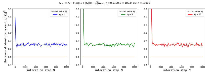
Figure 2. As $T=100$, simulations values of the second absolute moment $\mathbb{E}\left|Y_{k}\right|^{2}$ for the EM scheme (3.1) with initial $Y_{0}=1,5,10$, $\eta=0.01$ and iteration steps $n=10\,000$, $0\leqslant k\leqslant n$.

Figures 1 and 2 indicate that $\{\mathbb{E}\left|Y_{k}\right|^{2},k\leqslant n\}$ are bounded and has a clear decreasing trend with respect to $0\leqslant k\leqslant n$ for each initial value and step size.

For SDE (1.2) with $\alpha\in(0,2)$ and the corresponding EM scheme (1.7), due to the condition of $K_{2}$ in the proof of Theorem 1.2, we choose $T=100$ here. And we consider three cases, that is, $\alpha=0.5,1.0$, and $1.5$. For each case, we let $\beta$ be $\frac{\alpha}{8}$, $\frac{\alpha}{4}$ and $\frac{\alpha}{2}$. The simulated values of the $\beta$-th moment of $\widetilde{Y}_{n}$ in these cases are listed in Tables 1, 2, and 3.

Table 1. Simulated values of the absolute moment for the EM scheme (1.7) with $T=100$, $\alpha=0.50$ and $n=\{100,105,110,\dotsc,145\}$.

$n$	$\mathbb{E}|{\widetilde{Y}_{n}}|^{{\alpha}/{8}}$	$\mathbb{E}|{\widetilde{Y}_{n}}|^{{\alpha}/{4}}$	$\mathbb{E}|{\widetilde{Y}_{n}}|^{{\alpha}/{2}}$
$100$	$1.8\times 10^{13}$	$6.2\times 10^{26}$	$3.8\times 10^{55}$
$105$	$6.5\times 10^{13}$	$1.3\times 10^{28}$	$4.7\times 10^{57}$
$110$	$2.8\times 10^{14}$	$3.0\times 10^{29}$	$3.6\times 10^{60}$
$115$	$1.2\times 10^{15}$	$5.4\times 10^{30}$	$1.6\times 10^{63}$
$120$	$5.5\times 10^{15}$	$1.3\times 10^{32}$	$4.3\times 10^{65}$
$125$	$2.4\times 10^{16}$	$2.1\times 10^{33}$	$1.7\times 10^{68}$
$130$	$1.1\times 10^{17}$	$4.5\times 10^{34}$	$1.3\times 10^{71}$
$135$	$1.5\times 10^{18}$	$\infty$	$\infty$
$140$	$\infty$	$\infty$	$\infty$
$145$	$\infty$	$\infty$	$\infty$

Table 2. Simulated values of the absolute moment for the EM scheme (1.7) with $T=100$, $\alpha=1.0$ and $n=\{100,105,110,\dotsc,145\}$.

$n$	$\mathbb{E}|{\widetilde{Y}_{n}}|^{{\alpha}/{8}}$	$\mathbb{E}|{\widetilde{Y}_{n}}|^{{\alpha}/{4}}$	$\mathbb{E}|{\widetilde{Y}_{n}}|^{{\alpha}/{2}}$
$100$	$3.8\times 10^{25}$	$7.1\times 10^{52}$	$2.2\times 10^{109}$
$105$	$7.7\times 10^{26}$	$1.5\times 10^{55}$	$2.3\times 10^{112}$
$110$	$1.3\times 10^{28}$	$1.1\times 10^{58}$	$5,4\times 10^{117}$
$115$	$2.7\times 10^{29}$	$2.2\times 10^{60}$	$2.7\times 10^{124}$
$120$	$4.6\times 10^{30}$	$1.3\times 10^{63}$	$6.3\times 10^{128}$
$125$	$9.2\times 10^{31}$	$3.9\times 10^{65}$	$1.2\times 10^{135}$
$130$	$1.7\times 10^{33}$	$2.9\times 10^{68}$	$2.1\times 10^{141}$
$135$	$2.9\times 10^{34}$	$3.7\times 10^{71}$	$1.9\times 10^{145}$
$140$	$5.9\times 10^{35}$	$1.8\times 10^{73}$	$\infty$
$145$	$\infty$	$\infty$	$\infty$

Table 3. Simulated values of the absolute moment for the EM scheme (1.7) with $T=100$, $\alpha=1.5$ and $n=\{100,105,110,\dotsc,145\}$.

$n$	$\mathbb{E}|{\widetilde{Y}_{n}}|^{{\alpha}/{8}}$	$\mathbb{E}|{\widetilde{Y}_{n}}|^{{\alpha}/{4}}$	$\mathbb{E}|{\widetilde{Y}_{n}}|^{{\alpha}/{2}}$
$100$	$8.7\times 10^{37}$	$8.4\times 10^{77}$	$7.0\times 10^{158}$
$105$	$5.8\times 10^{39}$	$5.6\times 10^{83}$	$7.8\times 10^{168}$
$110$	$3.9\times 10^{41}$	$3.7\times 10^{86}$	$6.9\times 10^{174}$
$115$	$2.7\times 10^{43}$	$1.4\times 10^{90}$	$2.1\times 10^{182}$
$120$	$2.9\times 10^{45}$	$6.0\times 10^{93}$	$4.6\times 10^{192}$
$125$	$1.9\times 10^{47}$	$2.4\times 10^{97}$	$1.8\times 10^{200}$
$130$	$3.3\times 10^{49}$	$4.8\times 10^{101}$	$8.7\times 10^{207}$
$135$	$4.7\times 10^{51}$	$7.2\times 10^{104}$	$7.1\times 10^{215}$
$140$	$2.9\times 10^{53}$	$2.5\times 10^{111}$	$9.2\times 10^{219}$
$145$	$\infty$	$\infty$	$\infty$

From Tables 1, 2, and 3, we observe that the simulated values of the absolute moments of $\widetilde{Y}_{n}$ increase with respect to number of iteration $n$. In addition, they suggest that, for smaller values of $\alpha\in(0,1)$, lager values of time $T$ should be chosen due to constant $\kappa_{\alpha}=(2^{\alpha}/(2^{\alpha}-1))$ in Lemma 2.2. Consequently, these tables indicate that the behavior of the absolute $\frac{\alpha}{2}$-th moment varies with respected to $\alpha$ if we choose a fixed time $T$.

6. Appendix: The existence and uniqueness of strong solution

Since the diffusion coefficient function $f(x)=-x\log(1+|x|)$ in SDE (1.2) is only locally Lipschitz and satisfies the local growth condition in [1], Theorem 6.2.11 in [1] implies that (1.2) has a unique local solution. The following theorem strengthens this result by proving the existence and uniqueness of strong global solution of SDE (1.2).

Theorem 6.1.

SDE (1.2) has an unique strong global solution. Moreover, if $\alpha=2$, we have

$$\mathbb{E}|X_{t}|^{2}<\infty,\quad\forall\ t>0;$$

if $\alpha\in(0,2)$, then for every $\beta\in(0,\alpha)$,

$$\mathbb{E}|X_{t}|^{\beta}<\infty,\quad\forall\ t>0.$$

By adopting the argument in [11, Section 1.6], we can show the theorem for the case of $\alpha=2$. This argument can be extended to prove the theorem for the case of $\alpha\in(0,2)$. However, we have not been able to find a proof in the literature. For completeness, we provide a proof of Theorem 6.1.

Since the coefficient function $f(x)=-x\log(1+\left|x\right|)$ is a local Lipschitz function, For every $n\in\mathbb{N}_{+}$, we define the following truncated function $f_{n}(x)$ on $\mathbb{R}^{d}$ by

$$f_{n}(x)=\begin{cases}-x\log(1+\left|x\right|),\ \ \ \ &\left|x\right|\leqslant n;\\ \ -x\log(1+n),&\left|x\right|>n.\end{cases}$$

Proof.

By the definition of $f_{n}(x)$, it can been verified that $f_{n}(x)$ is a global Lipschitz function with linear growth. Hence, [1, Theorem 6.2.3] implies that the SDE

(6.1) $$\,\mathrm{d}X_{n,t}=f_{n}(X_{n,t})\,\mathrm{d}t+\,\mathrm{d}L_{t}$$

has a unique strong solution $F_{n}$, and

$$X_{n}(t,x,\omega):=F_{n}(x,\omega)(t).$$

Define a stopping time $\tau_{n}$ as

$$\tau_{n}=\inf\left\{t\geqslant 0:\left|X_{n,t}\right|\geqslant n\right\},\quad n\geqslant 2.$$

By the definition of $f_{n}(x)$, we have

$$\left\langle x,f_{n}(x)\right\rangle =-\left|x\right|^{2}\log(1+\left|x\right|)\mathbbm{1}_{[0,n]}(\left|x\right|)-\log(1+n)\left|x\right|^{2}\mathbbm{1}_{(n,\infty)}(\left|x\right|)$$

$$=-\left|x\right|^{2}\log(1+\left|x\right|)\big{(}\mathbbm{1}_{[0,\mathrm{e}-1]}(\left|x\right|)+\mathbbm{1}_{(\mathrm{e}-1],n}(\left|x\right|)\big{)}-\left|x\right|^{2}\mathbbm{1}_{(n,\infty)}(\left|x\right|)$$

$$\leqslant-\left|x\right|^{2}+1.$$

In the case of $\alpha\in(0,2)$, we define function $V(x):\mathbb{R}^{d}\to\mathbb{R}$ as

$$V_{\beta}(x)=\left(1+\left|x\right|^{2}\right)^{\beta/2},\quad\beta\in(0,\alpha).$$

Then we have

$$\nabla V_{\beta}(x) =\frac{\beta x}{(1+\left|x\right|^{2})^{1-\beta/2}}\ ,$$

$$\nabla^{2}V_{\beta}(x) =\frac{\beta\ {I}_{d}}{(1+\left|x\right|^{2})^{1-\beta/2}}+\frac{\beta(\beta-2)xx^{\prime}}{(1+\left|x\right|^{2})^{2-\beta/2}}\ ,$$

where $I_{d}$ is the identity matrix in $\mathbb{R}^{d\times d}$. Hence, for all $x\in\mathbb{R}^{d}$, we have $\left|x\right|^{\beta}\leqslant V_{\beta}(x)\leqslant 1+\left|x\right|^{\beta}$ and

$$\left|\nabla V_{\beta}(x)\right|\leqslant\beta\left|x\right|^{\beta-1},\quad\left\|\nabla^{2}V_{\beta}(x)\right\|_{\operatorname{HS}}\leqslant\beta(3-\beta)\sqrt{d}.$$

Besides, the following also holds for all $x\in\mathbb{R}^{d}$

$$\left\langle\nabla V_{\beta}(x),f_{n}(x)\right\rangle=\frac{\beta\left\langle x,f_{n}(x)\right\rangle}{(1+\left|x\right|^{2})^{1-\beta/2}}\leqslant-\beta V_{\beta}(x)+2\beta.$$

Itô’s formula yields that

(6.2) $$V_{\beta}(X_{n,t}) =V_{\beta}(x)+\int_{0}^{t}\left\langle\nabla V_{\beta}(X_{n,s}),f_{n}(X_{n,s})\right\rangle\,\mathrm{d}s$$

$$+ \int_{0}^{t}\int_{\left|z\right|<1}\left[V_{\beta}(X_{n,s}+z)-V_{\beta}(X_{n,s})\right]\widetilde{P}(\,\mathrm{d}s,\,\mathrm{d}z)$$

$$+ \int_{0}^{t}\int_{\left|z\right|\geqslant 1}\left[V_{\beta}(X_{n,s}+z)-V_{\beta}(X_{n,s})\right]P(\,\mathrm{d}s,\,\mathrm{d}z)$$

$$+ \int_{0}^{t}\int_{\left|z\right|<1}\left[V_{\beta}(X_{n,s}+z)-V_{\beta}(X_{n,s})-\left\langle\nabla V_{\beta}(X_{n,s}),z\right\rangle\right]\frac{C_{d,\alpha}\,\mathrm{d}z\,\mathrm{d}s}{\left|z\right|^{d+\alpha}}.$$

Before estimating $\mathbb{E}V_{\beta}(X_{n,t})$, we compute the following. If $\alpha\in(1,2)$, we let $\beta\in(1,\alpha)$, then we have that for any $x\in\mathbb{R}^{d}$

$$\mathrel{\phantom{=}}\int_{\mathbb{R}^{d}\backslash\{0\}}\left[V_{\beta}(x+z)-V_{\beta}(x)-\left\langle\nabla V_{\beta}(x),z\right\rangle\mathbbm{1}_{(0,1)}(\left|z\right|)\right]\frac{\,\mathrm{d}z}{\left|z\right|^{d+\alpha}}$$

$$=\int_{\left|z\right|\geqslant 1}\int_{0}^{1}\left\langle\nabla V_{\beta}(x+sz),z\right\rangle\frac{\,\mathrm{d}s\,\mathrm{d}z}{\left|z\right|^{d+\alpha}}+\int_{\left|z\right|<1}\int_{0}^{1}\int_{0}^{s}\left\langle\nabla^{2}V_{\beta}(x+uz),zz^{\prime}\right\rangle_{\mathrm{HS}}\frac{\,\mathrm{d}u\,\mathrm{d}s\,\mathrm{d}z}{\left|z\right|^{d+\alpha}}$$

$$\leqslant\beta\int_{\left|z\right|\geqslant 1}(\left|x\right|^{\beta-1}\left|z\right|+\left|z\right|^{\beta})\frac{\,\mathrm{d}z}{\left|z\right|^{d+\alpha}}+\beta(3-\beta)\sqrt{d}\int_{\left|z\right|<1}\left|z\right|^{2}\frac{\,\mathrm{d}z}{\left|z\right|^{d+\alpha}}$$

$$=\beta s_{d-1}\left(\frac{\left|x\right|^{\beta-1}}{\alpha-1}+\frac{1}{\alpha-\beta}\right)+\frac{\beta(3-\beta)s_{d-1}\sqrt{d}}{2(2-\alpha)}.$$

On the other hand, for $\alpha\in(0,1]$, we use the inequality $(a+b)^{\beta}\leqslant a^{\beta}+b^{\beta}$, where $\beta\in(0,1)$ and $a,b>0$, to derive

$$\mathrel{\phantom{=}}\int_{\left|z\right|\geqslant 1}\left[V_{\beta}(x+z)-V_{\beta}(x)\right]\frac{\,\mathrm{d}z}{\left|z\right|^{d+\alpha}}\leqslant\int_{\left|z\right|\geqslant 1}\left[1+\left|x+z\right|^{\beta}-\left|x\right|^{\beta}\right]\frac{\,\mathrm{d}z}{\left|z\right|^{d+\alpha}}$$

$$\leqslant\int_{\left|z\right|\geqslant 1}\frac{1+\left|z\right|^{\beta}}{\left|z\right|^{d+\alpha}}\,\mathrm{d}z=\frac{(2\alpha-\beta)s_{d-1}}{\alpha(\alpha-\beta)}.$$

Thus, an argument similar to that for the case $\alpha\in(1,2)$ implies that for $\alpha\in(0,1]$ and $\beta\in(0,\alpha)$,

$$\mathrel{\phantom{=}}\int_{\mathbb{R}^{d}\backslash\{0\}}\left[V_{\beta}(x+z)-V_{\beta}(x)-\left\langle\nabla V_{\beta}(x),z\right\rangle\mathbbm{1}_{(0,1)}(\left|z\right|)\right]\frac{\,\mathrm{d}z}{\left|z\right|^{d+\alpha}}$$

$$\leqslant\frac{(2\alpha-\beta)s_{d-1}}{\alpha(\alpha-\beta)}+\frac{\beta(3-\beta)s_{d-1}\sqrt{d}}{2(2-\alpha)}.$$

By combining the above inequalities with equation (6.2), we obtain that

$$\frac{\,\mathrm{d}\mathbb{E}V_{\beta}(X_{n,t})}{\,\mathrm{d}t} =\mathbb{E}[\left\langle\nabla V_{\beta}(X_{n,t}),f_{n}(X_{n,t})\right\rangle]$$

(6.3) $$+C_{d,\alpha} \mathbb{E}\left[\int_{\mathbb{R}^{d}\backslash\{0\}}[V_{\beta}(X_{n,t}+z)-V_{\beta}(z)-\left\langle\nabla V_{\beta}(X_{n,t}),z\right\rangle\mathbbm{1}_{(0,1)}(\left|z\right|)]\frac{\,\mathrm{d}z}{\left|z\right|^{d+\alpha}}\right]$$

$$\leqslant-\beta\mathbb{E}V_{\beta}(X_{n,t})+c_{1}\big{[}\mathbb{E}V_{\beta}(X_{n,t})^{\frac{\beta-1}{\beta}}\mathbbm{1}_{(1,2)}(\alpha)+\mathbbm{1}_{(0,1]}(\alpha)\big{]}+c_{2}$$

$$\leqslant-C_{1}\mathbb{E}V_{\beta}(X_{n,t})+C_{2},$$

where the first inequality follows from $\left|x\right|^{\beta-1}\leqslant V_{\beta}(x)^{(\beta-1)/\beta}$ as $\beta>1$, the second inequality from Hölder’s inequality, and $c_{1},c_{2},C_{1},C_{2}$ are constants independent of $t$ and $n$. Hence, for any $\alpha\in(0,2)$, the differential inequality (6) leads to

(6.4) $$\mathbb{E}V_{\beta}(X_{n,t})\leqslant V_{\beta}(x_{0})\mathrm{e}^{-C_{1}t}+C_{2}/C_{1}\leqslant C,\quad\forall\ t\geqslant 0.$$

Due to the definition of $V_{\beta}(x)$, we know that

$$V_{\beta}(X_{n,\tau_{n}})\geqslant(n^{2}+1)^{\frac{\beta}{2}},$$

then for any $T>0$, (6.4) and Markov’s inequality lead to

$$(n^{2}+1)^{\frac{\beta}{2}}\mathbb{P}(\tau_{n}\leqslant T)\leqslant\mathbb{E}\left[V_{\beta}(X_{n,\tau_{n}})\mathbbm{1}_{\tau_{n}\leqslant T}\right]\leqslant C.$$

Let $n\to\infty$, we obtain

$$\mathbb{P}(\lim_{n\to\infty}\tau_{n}\leqslant T)=0,$$

This and the arbitrariness of $T$ imply

(6.5) $$\lim_{n\to\infty}\tau_{n}=\infty.$$

As a result, (6.5) yields that $\forall x\in\mathbb{R}^{d},t\geqslant 0$,

$$X(t,x,\omega)=\lim_{n\to\infty}X_{n}(t,x,\omega)$$

exists and is continuous with respect to $(t,x)$, which is a solution of SDE (1.2). On the other hand, let $X(t)$ and $Y(t)$ be solutions with the same initial value $x$. Define

$$\gamma_{n}=\inf\{t:\left|X(t)\right|\geqslant n\},\quad\theta_{n}=\inf\{t:\left|Y(t)\right|\geqslant n\}.$$

Then, we have

$$X(\gamma_{n}\land\theta_{n}\land t)-Y(\gamma_{n}\land\theta_{n}\land t)=\int_{0}^{t}f_{n}(X(\gamma_{n}\land\theta_{n}\land s))-f_{n}(Y(\gamma_{n}\land\theta_{n}\land s))\,\mathrm{d}s,$$

which implies that

$$\mathrel{\phantom{=}}\mathbb{E}\left|X(\gamma_{n}\land\theta_{n}\land t)-Y(\gamma_{n}\land\theta_{n}\land t)\right|$$

$$\leqslant\left\|f_{n}\right\|_{\operatorname{Lip}}\int_{0}^{t}\mathbb{E}\left|X(\gamma_{n}\land\theta_{n}\land s)-Y(\gamma_{n}\land\theta_{n}\land s)\right|\,\mathrm{d}s.$$

Then by Grönwall’s inequality, we have that

$$\mathbb{E}\left|X(\gamma_{n}\land\theta_{n}\land t)-Y(\gamma_{n}\land\theta_{n}\land t)\right|=0,\quad\forall\ t\geqslant 0,$$

which implies that $X(t)=Y(t)$ on $t\leqslant\gamma_{n}\land\theta_{n}$. Then, let $n\to\infty$, we have $\gamma_{n}\land\theta_{n}\to\infty,a.s.$. Hence, $X(t)=Y(t),a.s.$ for all $t\geqslant 0$.

Finally, for the moment estimation, by the same argument for bounding $\mathbb{E}V_{\beta}(X_{n,t})$, we can establish that $\mathbb{E}V_{\beta}(X_{t})\leqslant C$ for all $t>0$, where $C>0$ is a constant not depending on $t$. This implies that $\mathbb{E}\left|X_{t}\right|^{\beta}\leqslant\mathbb{E}V_{\beta}(X_{t})\leqslant C$ for all $\beta\in(0,\alpha)$ and $t>0$. This completes the proof. ∎

References

- [1] David Applebaum. Lévy processes and stochastic calculus, volume 116 of Cambridge Studies in Advanced Mathematics. Cambridge University Press, Cambridge, second edition, 2009.
- [2] Ari Arapostathis, Hassan Hmedi, Guodong Pang, and Nikola Sandrić. Uniform polynomial rates of convergence for a class of Lévy-driven controlled SDEs arising in multiclass many-server queues. In Modeling, stochastic control, optimization, and applications, volume 164 of IMA Vol. Math. Appl., pages 1–20. Springer, Cham, 2019.
- [3] Khaled Bahlali, Antoine Hakassou, and Youssef Ouknine. A class of stochastic differential equations with super-linear growth and non-Lipschitz coefficients. Stochastics, 87(5):806–847, 2015.
- [4] Jianhai Bao, Xing Huang, and Chenggui Yuan. Convergence rate of Euler-Maruyama scheme for SDEs with Hölder-Dini continuous drifts. J. Theoret. Probab., 32(2):848–871, 2019.
- [5] Jianhai Bao and Jian Wang. Coupling approach for exponential ergodicity of stochastic Hamiltonian systems with Lévy noises. Stochastic Process. Appl., 146:114–142, 2022.
- [6] Jianhai Bao, George Yin, and Chenggui Yuan. Two-time-scale stochastic partial differential equations driven by -stable noises: averaging principles. Bernoulli, 23(1):645–669, 2017.
- [7] Jianhai Bao and Chenggui Yuan. Comparison theorem for stochastic differential delay equations with jumps. Acta Appl. Math., 116(2):119–132, 2011.
- [8] Jianhai Bao and Chenggui Yuan. Stochastic population dynamics driven by Lévy noise. J. Math. Anal. Appl., 391(2):363–375, 2012.
- [9] R. M. Blumenthal and R. K. Getoor. Some theorems on stable processes. Trans. Amer. Math. Soc., 95:263–273, 1960.
- [10] Björn Böttcher, René Schilling, and Jian Wang. Lévy matters. III, volume 2099 of Lecture Notes in Mathematics. Springer, Cham, 2013. Lévy-type processes: construction, approximation and sample path properties, With a short biography of Paul Lévy by Jean Jacod, Lévy Matters.
- [11] Sandra Cerrai. Second order PDE’s in finite and infinite dimension, volume 1762 of Lecture Notes in Mathematics. Springer-Verlag, Berlin, 2001. A probabilistic approach.
- [12] J. M. Chambers, C. L. Mallows, and B. W. Stuck. A method for simulating stable random variables. J. Amer. Statist. Assoc., 71(354):340–344, 1976.
- [13] Peng Chen, Chang-Song Deng, René L. Schilling, and Lihu Xu. Approximation of the invariant measure of stable SDEs by an Euler-Maruyama scheme. Stochastic Process. Appl., 163:136–167, 2023.
- [14] Peng Chen, Xinghu Jin, Yimin Xiao, and Lihu Xu. Approximation of the invariant measure for stable SDE by the Euler-Maruyama scheme with decreasing step-sizes. arXiv preprint arXiv:2310.05390, 2023.
- [15] Peng Chen, Ivan Nourdin, Lihu Xu, and Xiaochuan Yang. Multivariate stable approximation in Wasserstein distance by Stein’s method. arXiv preprint arXiv:1911.12917, 2019.
- [16] Zhen-Qing Chen and Xicheng Zhang. Heat kernels and analyticity of non-symmetric jump diffusion semigroups. Probab. Theory Related Fields, 165(1-2):267–312, 2016.
- [17] Thanh Dang and Lingjiong Zhu. Euler-Maruyama schemes for stochastic differential equations driven by stable Lévy processes with i.i.d. stable components. arXiv preprint arXiv:2402.12502, 2024.
- [18] Changsong Deng, Rene L Schilling, and Lihu Xu. Wasserstein- distance between SDEs driven by Brownian motion and stable processes. arXiv preprint arXiv:2302.03372, 2023.
- [19] Zhao Dong, Feng-Yu Wang, and Lihu Xu. Irreducibility and asymptotics of stochastic Burgers equation driven by -stable processes. Potential Anal., 52(3):371–392, 2020.
- [20] Shizan Fang and Tusheng Zhang. A class of stochastic differential equations with non-Lipschitzian coefficients: pathwise uniqueness and no explosion. C. R. Math. Acad. Sci. Paris, 337(11):737–740, 2003.
- [21] Peter Hall. Two-sided bounds on the rate of convergence to a stable law. Z. Wahrsch. Verw. Gebiete, 57(3):349–364, 1981.
- [22] Desmond J. Higham, Xuerong Mao, and Andrew M. Stuart. Strong convergence of Euler-type methods for nonlinear stochastic differential equations. SIAM J. Numer. Anal., 40(3):1041–1063, 2002.
- [23] Desmond J. Higham, Xuerong Mao, and Andrew M. Stuart. Exponential mean-square stability of numerical solutions to stochastic differential equations. LMS J. Comput. Math., 6:297–313, 2003.
- [24] Martin Hutzenthaler, Arnulf Jentzen, and Peter E. Kloeden. Strong and weak divergence in finite time of Euler’s method for stochastic differential equations with non-globally Lipschitz continuous coefficients. Proc. R. Soc. Lond. Ser. A Math. Phys. Eng. Sci., 467(2130):1563–1576, 2011.
- [25] Martin Hutzenthaler, Arnulf Jentzen, and Peter E. Kloeden. Divergence of the multilevel Monte Carlo Euler method for nonlinear stochastic differential equations. Ann. Appl. Probab., 23(5):1913–1966, 2013.
- [26] Ioannis Karatzas and Steven E. Shreve. Brownian motion and stochastic calculus, volume 113 of Graduate Texts in Mathematics. Springer-Verlag, New York, second edition, 1991.
- [27] Panki Kim and Renming Song. Stable process with singular drift. Stochastic Process. Appl., 124(7):2479–2516, 2014.
- [28] Panki Kim, Renming Song, and Zoran Vondraček. Heat kernels of non-symmetric jump processes: beyond the stable case. Potential Anal., 49(1):37–90, 2018.
- [29] Peter E. Kloeden and Eckhard Platen. Numerical solution of stochastic differential equations, volume 23 of Applications of Mathematics (New York). Springer-Verlag, Berlin, 1992.
- [30] Franziska Kühn and René L. Schilling. Strong convergence of the Euler-Maruyama approximation for a class of Lévy-driven SDEs. Stochastic Process. Appl., 129(8):2654–2680, 2019.
- [31] Wei Liu, Renming Song, and Longjie Xie. Gradient estimates for the fundamental solution of Lévy type operator. Adv. Nonlinear Anal., 9(1):1453–1462, 2020.
- [32] Xuerong Mao and Lukasz Szpruch. Strong convergence and stability of implicit numerical methods for stochastic differential equations with non-globally Lipschitz continuous coefficients. J. Comput. Appl. Math., 238:14–28, 2013.
- [33] Olivier Menoukeu Pamen and Dai Taguchi. Strong rate of convergence for the Euler-Maruyama approximation of SDEs with Hölder continuous drift coefficient. Stochastic Process. Appl., 127(8):2542–2559, 2017.
- [34] John P. Nolan. Univariate stable distributions: models for heavy tailed data. Springer Series in Operations Research and Financial Engineering. Springer, Cham, 2020.
- [35] Bernt Ø ksendal. Stochastic differential equations. Universitext. Springer-Verlag, Berlin, sixth edition, 2003. An introduction with applications.
- [36] Daniel Revuz and Marc Yor. Continuous martingales and Brownian motion, volume 293 of Grundlehren der mathematischen Wissenschaften [Fundamental Principles of Mathematical Sciences]. Springer-Verlag, Berlin, 1991.
- [37] Ken-iti Sato. Lévy processes and infinitely divisible distributions, volume 68 of Cambridge Studies in Advanced Mathematics. Cambridge University Press, Cambridge, revised edition, 2013. Translated from the 1990 Japanese original.
- [38] Rong Situ. Theory of stochastic differential equations with jumps and applications. Mathematical and Analytical Techniques with Applications to Engineering. Springer, New York, 2005. Mathematical and analytical techniques with applications to engineering.
- [39] Bahram Tarami and Mohsen Avaji. Convergence of Euler-Maruyama method for stochastic differential equations driven by -stable Lévy motion. Journal of Mathematical Extension, 12(3):33–54, 2018.
- [40] Jian Wang. On the exponential ergodicity of Lévy-driven Ornstein-Uhlenbeck processes. J. Appl. Probab., 49(4):990–1004, 2012.
- [41] Chenggui Yuan and Xuerong Mao. Convergence of the Euler-Maruyama method for stochastic differential equations with Markovian switching. Math. Comput. Simulation, 64(2):223–235, 2004.
- [42] Chenggui Yuan and Xuerong Mao. A note on the rate of convergence of the Euler-Maruyama method for stochastic differential equations. Stoch. Anal. Appl., 26(2):325–333, 2008.