Modeling Sustainable City Trips: Integrating CO2 Emissions, Popularity, and Seasonality into Tourism Recommender Systems

Abstract.

In an era of information overload and complex decision-making processes, Recommender Systems (RS) have emerged as indispensable tools across diverse domains, particularly travel and tourism. These systems simplify trip planning by offering personalized recommendations that consider individual preferences and address broader challenges like seasonality, travel regulations, and capacity constraints. The intricacies of the tourism domain, characterized by multiple stakeholders, including consumers, item providers, platforms, and society, underscore the complexity of achieving balance among diverse interests. Although previous research has focused on fairness in Tourism Recommender Systems (TRS) from a multistakeholder perspective, limited work has focused on generating sustainable recommendations.

Our paper introduces a novel approach for assigning a sustainability indicator (SF index) for city trips accessible from the users’ starting point, integrating CO₂ emission analysis, destination popularity, and seasonal demand. Our methodology involves comprehensive data gathering on transportation modes and emissions, complemented by analyses of destination popularity and seasonal demand. A user study validates our index, showcasing its practicality and efficacy in providing well-rounded and sustainable city trip recommendations. Our findings contribute significantly to the evolution of responsible tourism strategies, harmonizing the interests of tourists, local communities, and the environment while paving the way for future research in responsible and equitable tourism practices.

1. Introduction

Recommender Systems (RS) provide tailored content to individual preferences, spanning diverse domains like e-commerce, social media, news, and more, effectively managing information to prevent overload (Abdollahpouri et al., 2020). In travel and tourism, RS is pivotal in simplifying trip planning by providing personalized recommendations for destinations, accommodations, activities, and more (Isinkaye et al., 2015). However, this is a particularly challenging domain due to the influence of dynamic factors such as seasonality and travel regulations (Balakrishnan and Wörndl, 2021), as well as constraints related to capacity-limited resources such as airline seats, hotel rooms, and event tickets (Abdollahpouri and Burke, 2021).

Traditionally, RS focused on delivering accurate user recommendations, but in practice, they function as a convergence point for multiple stakeholders, making it a multistakeholder scenario (Abdollahpouri et al., 2020). Recognizing the interests of all stakeholders becomes crucial in this dynamic. Our stakeholder classification, inspired by Balakrishnan and Wörndl (2021), identifies four key categories: consumers, item providers, platform, and society, aligning with common touristic recommendation scenarios. Despite this seemingly straightforward categorization, real-world stakeholder relationships are often more intricate. Each stakeholder is vested in the traveler’s journey, and optimizing consumer recommendations can yield benefits for all involved parties (Abdollahpouri et al., 2020). Complexities arise as the goals of one stakeholder may clash with another, leading to inevitable trade-offs (Jannach and Bauer, 2020). Thus, achieving fairness in Tourism Recommender Systems (TRS) requires adopting a multistakeholder approach, acknowledging stakeholders’ interdependence and balancing their objectives.

Tourism’s impact goes beyond active participants, affecting the local environment and businesses and profoundly influencing the balance of nature. Constructing a fair TRS involves recommending sustainable options and fostering responsible tourism practices. World Tourism Organization and United Nations Development Programme define sustainable tourism as ”tourism that takes full account of its current and future economic, social and environmental impacts, addressing the needs of visitors, the industry, the environment, and host communities”  (Gössling, 2017). Achieving sustainability in tourism requires interventions at various levels, including municipal policies and regulations (Werthner et al., 2015). However, measuring sustainability at destinations poses a significant challenge, impeding effective decision-making, management, and meeting destination needs (Fernández and Rivero, 2009). A destination’s sustainability is crucial for long-term competitiveness and visitor satisfaction, not solely determined by arrival numbers or bed nights (Irem et al., 2017).

Regulating tourist numbers is a crucial intervention to manage the impact of tourism, and this is where a well-designed TRS can play a vital role. Such a system proves particularly beneficial in addressing the twin challenges of overtourism and undertourism, both on the rise due to factors like low-cost aviation, affordable transportation, social media influence, and platforms like Airbnb  (Gowreesunkar and Vo Thanh, 2020). Overtourism, witnessed in popular destinations like Venice, Barcelona, Rome, and Dubrovnik, poses threats to historic preservation, the environment, residents, and overall tourist experiences, making it challenging to find reasonably priced housing in these cities (Dastgerdi and De Luca, 2023; Dodds and Butler, 2019). Conversely, undertourism, prevalent in under-explored destinations, results from a lack of infrastructure, publicity, and accessibility. Both scenarios have adverse consequences. For instance, the recent COVID-19 pandemic highlighted the adverse effects of undertourism, causing significant disruptions to the tourism and hotel industries (Galí, 2022). To address these issues, a TRS must be designed to provide responsible recommendations, considering the interests of all stakeholders. These systems should advocate for sustainable tourism practices, promoting responsible tourism while offering personalized suggestions to users. This involves recommendations encouraging tourists to visit destinations with minimal environmental impact, promoting less popular yet attractive locations, and balancing the tourist load uniformly throughout the year. In the context of this paper, we use the terms sustainability and responsibility interchangeably.

A substantial amount of research has been conducted on developing fair recommendation systems that consider the interests of all stakeholders involved in tourism  (Rahmani et al., 2022; Shen et al., 2021; Weydemann et al., 2019; Wu et al., 2021). However, there has been limited focus on generating sustainable recommendations (Banerjee et al., 2023). This paper delves into the concept of modeling Societal Fairness or S-Fairness, emphasizing the impact of tourism on individuals not directly involved, such as residents, environment, etc. (Banerjee, 2023). These stakeholders often encounter challenges such as rising housing prices, environmental pollution, and traffic congestion due to heightened tourism activities in their vicinity.

In the context of tourism, a destination is characterized by ”a country, state, region, city, or town that is actively marketed or markets itself as an appealing place for tourists to visit” (Beirman, 2020). For this paper, we designate destinations as a compilation comprising the 200 most densely populated European cities. Our focus is on assisting travelers seeking vacation recommendations for visiting these cities from their respective starting points. We propose a method to measure sustainability at destinations relative to the users’ starting point by assigning a composite S-Fairness index (SF index) to all cities accessible from the users’ initial location.

To mitigate the adverse effects on the environment and society, we identify three key factors in the calculation of the SF index:

• Destinations with environmentally friendly travel options, minimizing CO₂ emissions incurred during the travel to the destination.

• Suggesting less popular yet attractive destinations.

• Choosing destinations with lower demand during the specific month.

Our approach is designed to assist travelers in making more sustainable travel choices. As depicted in Figure 1, an example user interface shows the top travel recommendations from Munich (Germany) for July. The SF index is featured in the top right corner, accompanied by its components, including emissions, travel time for each mode of transport, aggregated popularity, and seasonal demand of each city for the month. Such an application can assist users in making informed decisions. A lower overall index for a city indicates a more environmentally friendly travel option from the user’s starting point. This paper delves into the methodology behind collecting the information in the figure. Showcasing the SF index for analyzing specific tourist destinations provides a concrete perspective on their sustainability status, encouraging responsible tourism practices crucial for the well-being of communities and the environment.

To this end, our work makes the following contributions:

• Defining the concept of sustainability and its elements within a city trip recommender system.

• Collecting and examining data on transportation CO₂ emissions, as well as determining popularity and seasonality indices for cities. This involves assigning a composite SF index to cities based on a specific starting point and month of travel.

• Executing a user study to explore fundamental travel trade-offs and ascertain the SF index weights.

• Verifying the effectiveness of our newly introduced SF index through an additional user study to assess its appropriateness.

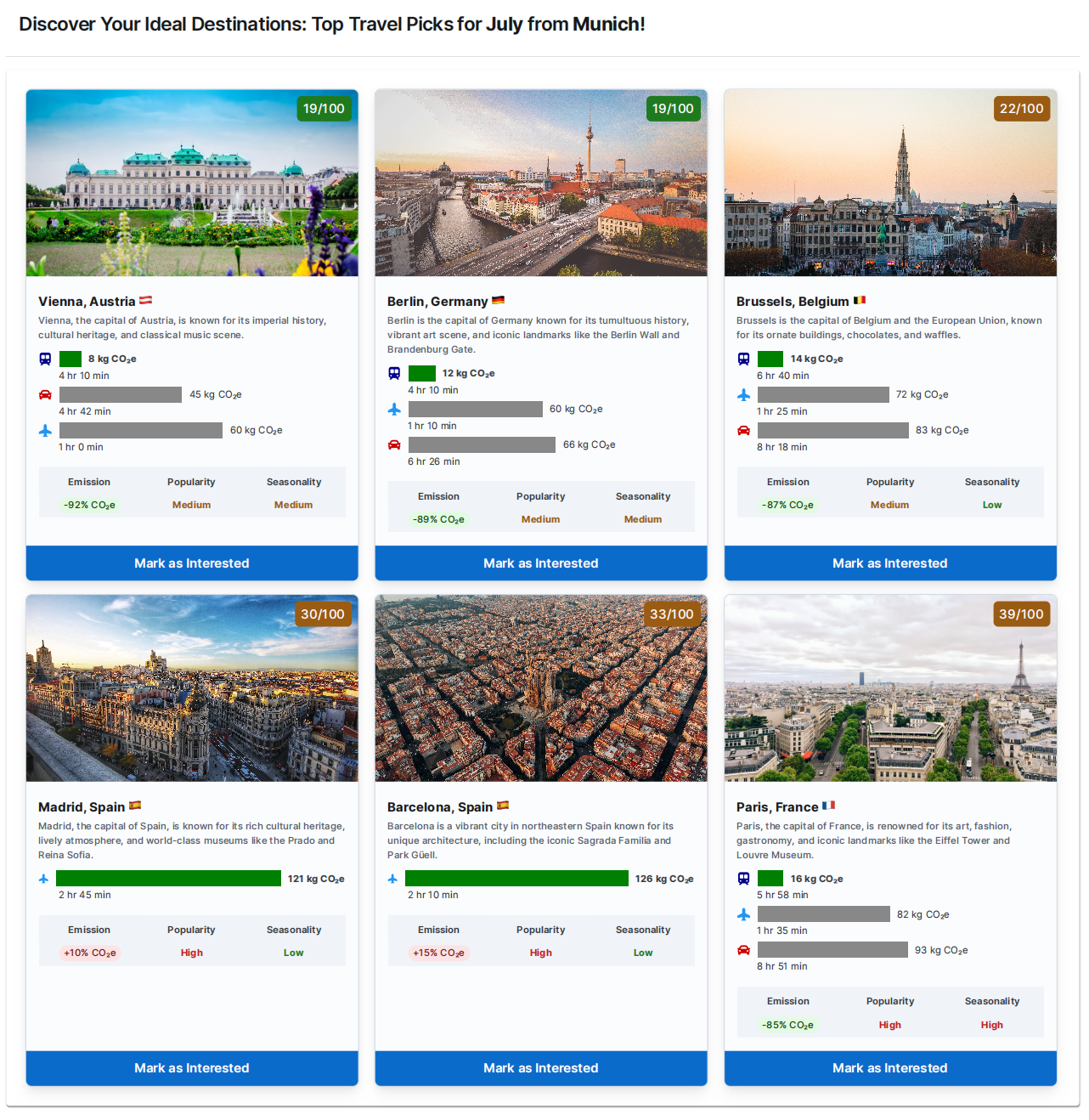
Figure 1. An example user interface showing top travel recommendations from Munich, Germany, for July while highlighting the S-Fairness index in the top right corner

Our paper is structured as follows: Section 2 reviews prior research on city trip recommendations and sustainability promotion. In Section 3, we detail methodologies for calculating transportation-related CO₂ emissions.  Section 4 outlines methods for estimating city popularity and data collection.  Section 5 explores seasonal demand for the destinations.  Section 6 presents findings from a user study on factors influencing destination choices and openness to sustainable tourism recommendations, offering empirical insights. In Section 7, we elucidate the concept of Societal Fairness, assign the relevant indices, and subsequently validate our index through a dedicated user study. Finally, Section 8 concludes the paper, summarizing key findings and suggesting future studies in sustainable tourism and city trip planning.

2. Related Work

In the context of this study, related work encompasses two dimensions: city trip recommendations and sustainable recommendations, often referred to as S-Fairness. This reflects the evolving paradigm in recommender systems where personalization and user preference in city trip recommendations are increasingly integrated with the broader and critical perspective of sustainability and societal fairness.

City trip recommender systems have traditionally focused on modeling user preferences to deliver personalized recommendations. Techniques like collaborative filtering are prevalent, leveraging users’ past activities, similarities with other users, and network-based preferences (Lu et al., 2012; Dadoun et al., 2019; Massimo and Ricci, 2019). Constraints defined by users, such as budget or time preferences, are also critical components in tailoring travel packages (Xie et al., 2010; Lim et al., 2015). However, challenges like the cold start problem and data sparsity have led to the adoption of content-based approaches. These approaches construct domain models using relevant features for tourism, often derived from expert opinions, literature, or data-driven methods (Liu et al., 2011; Pu et al., 2020). While expert-driven models offer nuanced insights, their cost and complexity necessitate complementing them with diverse data sources, such as Location-based Social Networks (LBSNs) for venue data (Lu et al., 2012; Dadoun et al., 2019).

Sustainable tourism is a complex concept such that defining objectives and indicators for a sustainable TRS can be complicated. Ko (2005) claim that concerns on sustainability vary between destinations, hence dimensions for sustainability along with the methodology and data gathering should be particular to the destination. In respond to this approach the issue of comparability arises, where meaningful insights from comparing measurement between destination can’t be done since the sets of indicators are different. To address this, Cernat and Gourdon (2012) formulate the Sustainable Tourism Benchmarking Tool (STBT) comprises 54 indicators along seven dimensions (assets, activities, linkages, leakages, sustainability, attractiveness, and infrastructure). The interactions of these indicators are then tested on 75 countries but only perform well in Indonesia, Malaysia, and Thailand, where the data for most indicators is available. Conversely, Hoffmann et al. (2022) took a fully data-driven approach by analyzing data from TripAdvisor to make sense of the sustainability measurement between hotels with the sustainable label granted by the platform and those without. The study conducts unsupervised statistical learning to classify sustainable hotels by their features. The model results in significantly higher performance compared to random draw but the explainability of the model is not adequate. For instance, it is shown that larger hotels are more likely to be sustainable but it can’t be inferred as explicitly causal. It is heavily noted that the model can only be used as a probabilistic estimate to label sustainable destinations. Such methods might reveal relevant aspects of sustainability as well as solve the comparability issue however it is constrained by the completeness of the dataset and hard to generalize beyond the determined item space.

Irem et al. (2017) argues that it is more feasible to analyze existing sustainable tourism indicators than to introduce new measures lacking in direct practical applicability. Gorantla and Bansal (2023) adopt the Circles of Sustainability framework to describe how sustainable a city is. It measures sustainability along four domains –– ecology, economics, politics, and culture, with seven subdomains under each domain. The study then consolidates different data sources for each subdomain, which in the end used to calculate the sustainability index calculator. The sustainability index is calculated by summing up all the subdomain scores with equal weights and then normalizing them. Although the algorithm is simple, it gives a good outlook on the sustainability of a city compared to the others. Irem et al. (2017) proposes implementing data envelopment analysis (DEA) on existing tourism information systems to model destination competitiveness. DEA allows one to identify the efficiency of a destination, as well as benchmark it to another destination to give clues on which aspects can be improved. These studies show that it is possible to adopt existing frameworks into a partial model of city sustainability. The utility function, for instance, the sustainability index, can be calculated using the model and is useful to nudge policymakers and city developers to improve specific aspects of the city.

While numerous studies explore the quantification of sustainability in tourism, there is a notable scarcity of their application within recommender systems in this domain. Sustainable recommender system seeks to create a balance across economic, environmental, and social dimensions which is essential for creating a resilient ecosystem (Gorantla and Bansal, 2023). One can initiate the integration of features that capture user interest while simultaneously promoting sustainability. In the work by Herzog et al. (2019), attributes such as air quality, greenery, traffic, and pollution are employed to model the appeal of a travel route. The research demonstrates that tourists exhibit a preference for visually appealing routes, even if they entail longer travel distances Indirectly, the recommender system improves the distribution of tourists by suggesting less congested routes, also serving as a nudge to cities to develop more attractive alternative routes.

However, a sustainable recommender system should not be fully user-centric. The tourism industry involves different stakeholders, including consumers, providers, platforms, and society, thus it is natural for sustainable RS to implement a multistakeholder approach. Merinov et al. (2022) introduces a multistakeholder model that not only considers user preferences but also the occupancy level of the destination. In another study by Patro et al. (2020), the multi-objective model focuses on providers’ sustainability by maintaining their exposure while also preventing overcrowding. Pachot et al. (2021) added local authorities as stakeholders, with economic growth, productive resilience, prioritizing basic necessities, and greener production as its objective. In a recent examination of multistakeholder fairness within tourism recommender systems, it became apparent that existing studies predominantly concentrate on provider and consumer stakeholders. Surprisingly, the societal aspect, despite bearing significant impacts from tourism, is often overlooked as a stakeholder (Banerjee et al., 2023).

Our methodology differs from the state-of-the-art in terms of data collection and analysis techniques. We employ a combination of qualitative insights from participant feedback and quantitative data from various sources. This approach allows for a more nuanced understanding of tourist behavior and preferences, leading to more effective recommendations for city trip planning that align with S-Fairness principles.

3. Destinations, Transportation, and Emission Estimations

One of the crucial sustainability indicators in tourism, pertinent for city tourism policymakers, encompasses factors such as CO₂ emissions associated with travel to/from the city, the mix of transportation modes chosen by guests, the average distance covered by travelers to reach their destination, and the average length of stay, as highlighted by Önder et al. (2017). For example, longer-distance trips that necessitate air travel between cities tend to incur higher emissions, posing a more significant environmental impact than shorter trips feasible with public transport like trains. Conversely, a short-distance trip by car may result in more emissions than a train.

This paper adopts the estimation of greenhouse gases (GHG) emitted by various transportation modes to indicate the trip’s environmental responsibility concerning the travelers’ starting point. We examine the trade-off between travel times, transportation modes, their respective emissions, and the associated costs. Our approach encourages travelers to opt for public transport, particularly for shorter to medium-distance destinations. Ultimately, we assign an emission trade-off indicator $\mathit{Z(c_{i})}$ to each city $\mathit{c_{i}}$ reachable from the user’s point of origin. Analyzing trade-off values provides insights into user behavior, enabling the formulation of effective policies. These policies might include strategies to improve travel time on routes with lower emissions but higher costs. A lower $\mathit{Z(c_{i})}$ indicates a more environmentally friendly and responsible tourism approach.

Subsequent sections delve into detailed discussions on these aspects.

3.1. Extracting Destinations

In our scenario, a traveler is seeking a suitable city to visit for vacation from a specified starting location. The initial step involves collecting data on potential destinations for city trips. The experimental evaluation has been conducted on diverse datasets. Our item space comprises 200 European cities or destinations, spanning across 43 countries, chosen due to Europe’s extensive connectivity through various modes of transportation—flights, rail, and road—making it a prominent destination for tourism.

Data for European cities is sourced from the world cities database (World Cities Database, 2023), filtering for cities in Europe within latitudes 35°N to 72°N and longitudes 25°W to 65°E, with a population exceeding 100,000. The top 200 most populated cities, each featuring at least one airport, are selected. In our data, Moscow followed by Istanbul has the highest population, Ancona, and Klagenfurt have the lowest. Subsequently, we calculate transportation emissions for travel to each city using three modes — flights, driving, and rail where applicable as explained below. Figure 2 illustrates the geographical dispersion of the 200 European cities, each possessing at least one airport. It also shows the subset of cities specifically chosen for in-depth examination regarding driving and train connections in this study.

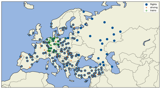
Figure 2. The geographical distribution of 200 European cities with at least one airport is depicted in blue, cities prioritized for driving highlighted in orange, and those considered for their train networks shown in green

3.2. Data Gathering: Transportation

3.2.1. Flights

In obtaining flight information, a major step involves associating cities with their respective airport details and IATA  codes. We gathered data from the Flugzeuginfo.net  website, aligning the information with our city list. Notably, cities featuring multiple international airports were also incorporated into the dataset. This resulted in a compilation of 222 unique airports across 200 cities. 14 cities with more than one airport, including Baku, Berlin, Copenhagen, Hamburg, Istanbul, London, Lyon, Madrid, Milan, Minsk, Moscow, Paris, Rome, and Stockholm were also modeled.

We established connections between airports $\mathit{a_{1}}$ and $\mathit{a_{2}}$, corresponding to cities $\mathit{c_{1}}$ and $\mathit{c_{2}}$, respectively. A dedicated connection was established for each unique route between the two cities, resulting in 16,261 unique one-way routes. It is important to clarify that the calculation of unique routes did not account for connections to return, although data for return connections was also gathered. Subsequently, each connection served as input for querying Google Flights , allowing us to extract detailed information. We prioritized the best departing flight options based on criteria such as travel time and number of stops for each trip, focusing on economy class. The gathered data included information on flight carriers, departure and arrival timings, the number of stops, and the duration of the flights.

We classified each route based on the Eurocontrol’s  definition for distances, segmenting them into four categories: very short haul, short haul, medium haul, and long haul. Specifically, very short-haul flights covered less than 500 km, short-haul flights ranged from 500 to 1,500 km, medium-haul flights spanned 1,500 to 4,000 km, and long-haul flights exceeded 4,000 km in flying distance. The scraped data from Google Flights lacked information on the distances between the two cities. Therefore, we employed the Great Circle Distance (GCD) (Wikipedia, 2023a, b) measurement to calculate the distances for each route. As indicated in Table 1, our dataset predominantly comprised short-haul and medium-haul flights, with a comparatively smaller number of long-haul flights.

We observed specific distance and duration patterns among different city pairs in analyzing various flight categories. Examples include Copenhagen to Malmö, showcasing the minimum distance in very short-haul flights, and Paris to Stuttgart having the minimum distance in short-haul flights. For medium-haul flights, Adana to Podgorica exhibited the minimum distance, while Ufa to Sevilla presented the maximum. In long-haul flights, Erzincan to Braga showed the minimum distance, while Baku to Nantes recorded the maximum. For a detailed overview of the numerical aspects, including minimum, maximum, and mean values for travel time, distances, and emissions (CO₂e) in each category, please refer to Table 1.

3.2.2. Driving

We assume that driving between cities is not viable when the distance is above 1,000 kilometers, so we eliminate the longer connections between city pairs. This refinement yielded 10,056 unique (two-way) connections spanning 200 European cities. We derived the driving distance and travel time for these connections using two prominent data sources.

Initially, we leveraged the Google Maps Routes API  in the eco-friendly mode to acquire the most fuel-efficient driving distance and time, factoring in real-time traffic conditions. However, due to cost constraints for larger datasets and limited availability in some countries, we obtained details for 4,718 unique one-way routes.

Subsequently, we utilized the Open Source Routing Machine (OSRM) API  in driving mode to compute the driving distance and time between connections. OSRM, an open-source routing engine, relies on OpenStreetMap  data, providing information for all 1056 connections in our dataset. The overview of both datasets can be found in Table 1.

Both datasets contained data regarding distance, travel time, and specific route details between two cities. Furthermore, the Google Maps Routes API offered an estimate of the fuel consumption for each route. Upon conducting a comparative analysis, it was observed that Google and OSRM demonstrated a mean absolute percentage difference of 5.63% in their respective distance calculations. This divergence may be ascribed to the different methodologies employed by Google and OSRM in estimating distances, considering factors such as routes and traffic conditions. It is essential to note that this paper does not explore the accuracy assessment of each data source.

3.2.3. Trains

The railway network across Europe exhibits a diverse and country-specific management infrastructure. Unfortunately, no open-source API or standardized pan-European platform would enable us to aggregate data seamlessly from various railway networks. Consequently, our approach relied on country-specific rail networks, focusing on Germany due to easier data accessibility. We utilized web scraping techniques on the Bahn.Expert website to gather the necessary information. This platform uses the Deutsche Bahn APIs  to provide valuable insights into past and present data on trains and stations, particularly for Deutsche Bahn (DB) or German trains (Clasen, 2020). For instance, users can search for specific train lines and review all stops on a selected day along its route. Additionally, the website offers information on schedules and real-time data for the arrival and departure of trains.

In our data collection process, our primary emphasis was on three prominent long-distance train categories in Germany— Intercity (IC), EuroCity (EC), and Intercity-Express (ICE). This focus was chosen because these categories encompass most of the major cities in Germany and extend to significant cities in neighboring countries, including Amsterdam, Vienna, Basel, Brussels, and others as illustrated in Figure 2. The stations chosen for data extraction encompassed major locations in Germany such as Berlin, Dortmund, Erfurt, Frankfurt, Hamburg, Hannover, Karlsruhe, Köln, Mannheim, München, Nürnberg, and Stuttgart. As depicted in Figure 2, the dataset includes 566 unique stations, reflecting the wide geographical coverage of the resulting train network. With 26,390 trips and 386,367 observations, the dataset provides a detailed view of connections and train stops. This dataset comprises 64 EC, 106 IC, and 63 ICE train lines, ensuring a thorough representation. The data collection period extended from January 1, 2023, to May 31, 2023, providing a robust timeframe for capturing diverse train travel patterns and facilitating thorough analyses.

We chose to focus on the data from DB, as it offers valuable insights into connections with major cities in Germany and neighboring countries. However, it’s important to note that our methodologies are adaptable and can be extended to incorporate data from other train providers across different European regions.

Table 1. Summary of data sources and basic statistics for calculating emissions upon arrival at the destination along with the CO₂e  values used for each category

Mode	Data Sources	Category	# Unique Routes	Distance (km)			Travel Time (hrs)			CO2e (g/km)
				Min	Mean	Max	Min	Mean	Max
Flights	Google Flights	Very Short Haul	1,617	30.46	331.68	499.70	1.08	6.79	50.25	155
		Short-Haul	7,086	501.34	995.33	1,499.78	1.08	7.21	83.17	110
		Medium-Haul	7,450	1,500.42	2292.91	3,986.05	2.03	10.82	53.75	75
		Long-Haul	108	4,004.87	4,317.96	4,986.29	8.33	18.41	55.25	95
Driving	Google Maps API	–	4,718	47.24	851.51	2,440.34	0.77	10.14	35.24	96
	OSRM API	–	5,028	43.67	917.03	2,967.52	0.72	11.08	37.67
Trains	Deutsche Bahn	ICEs	104	116.17	524.75	849.67	2.10	6.85	10.88	24
		ICs	144	24.51	236.86	672.77	0.68	3.66	9.27
		ECs	101	30.77	350.17	779.25	0.68	5.95	14.15

3.3. Estimation of Emissions from Transportation Modes

The emission of greenhouse gases (GHGs) from transportation plays a pivotal role in contributing to environmental damage, serving as a significant driver of climate change and environmental degradation. Greenhouse gases, such as water vapor, carbon dioxide (CO₂), methane (CH₄), nitrous oxide (N₂O), and ozone (O₃), are atmospheric gases that absorb and re-emit heat, thereby maintaining the Earth’s atmosphere at a warmer temperature (Lashof and Ahuja, 1990). Among these, CO₂ is the most prevalent greenhouse gas emitted by human activities, both in quantity and its overall impact on global warming. While the term ”CO₂” is occasionally used as a shorthand reference for all greenhouse gases, this can lead to confusion. In this paper, we use ”carbon dioxide equivalent” or ”CO₂e,” collectively referring to multiple greenhouse gases as suggested by Brander and Davis (2012).

While there were discrepancies among individual studies regarding the exact emissions per kilometer, the overall consensus indicates that short-distance flights have a higher environmental impact. In contrast, trains and public transport significantly reduce CO₂ emissions. Our modeling employs an average approach, in line with the above consensus. Table 1 presents a summary of values used for CO₂e calculations across various transportation modes. The subsequent sections provide a detailed exploration of the emission calculation process and our assumptions for each mode of transportation.

3.3.1. Flights

Responsibility for aviation greenhouse gas emissions involves addressing several complexities. An additional challenge arises from the variability in passenger occupancy rates among aircraft. While some planes are full of charter passengers, others may operate with less than half of their seats occupied, particularly during scheduled flights. This discrepancy may necessitate considering a higher rate of CO₂ emissions for those flying in partly empty aircraft. Additionally, individuals traveling in Business Class or First Class contribute to a higher share of CO₂ emissions, as highlighted by Carbon Independent (2023).

In its analysis of CO₂ emissions from commercial aviation, the International Council on Clean Transportation (ICCT) offers a detailed breakdown of the carbon intensity, measured in grams of CO₂ emitted per passenger kilometer, highlighting variations based on flight distance (Graver et al., 2019). This variability stems from the fact that take-off demands a considerably higher energy input than a flight’s cruise phase. Consequently, for very short flights, the additional fuel required for take-off becomes more substantial when contrasted with the more fuel-efficient cruise phase. The ICCT also observes that shorter flights often involve less fuel-efficient aircraft. For an overview of various methods used to estimate greenhouse gas (GHG) emissions in the aviation sector, the study by Iken and Aguessy (2022) provides valuable insights.

Google Flights calculate emissions per person using various factors, including the GCD between origin and destination airports, aircraft type, fuel burn, and flight occupancy following the Tier 3 methodology for emission estimates outlined by the European Environment Agency (EEA) (Google, 2019). However, the calculation results in a per-passenger CO₂e  contribution, which can be misleading compared to the overall fuel consumption for the entire journey. To facilitate a fair comparison with alternative transportation modes, such as rail and driving, we adopt a distance-based estimation model proposed by Graver et al. (2019) for standard economy class flights. Table 1 displays the distinct CO₂e values applied to three flight categories, categorized according to the covered distance. We also add an extra 9% correctional adjustment factor to the great-circle distance to account for delays and indirect flight paths, as noted by DEFRA (2007).

3.3.2. Driving

Estimating driving emissions involves several factors: elevation, car model, fuel type, car size, number of occupants, and traffic conditions (Ghosh et al., 2020). Driving alone in a car, particularly one running on fossil fuels, contributes more emissions than carpooling or using an electric vehicle. Additionally, route variations, traffic, time of day, distance, and travel time can lead to variable GHG emissions. In our simplified scenario, we consider a small gasoline-powered car occupied by a single person, and we calculate the estimates based on the distance for both Google and OSRM data. To calculate the CO₂e for the given route, we utilize the per-kilometer emission estimation from Ian Tiseo (2023), which is set at 96 grams per kilometer.

The Google data also included fuel consumption estimates, allowing us to derive the CO₂e values. We also compute the fuel consumption-based CO₂e for the Google data, with an emission rate of 2.3 kilograms of CO₂ per liter of gasoline (Hilali and Belmaghraoui, 2019). The mean absolute difference percentage of 10.90 between CO₂e values calculated from per-kilometer distance and those derived from fuel consumption estimates for the Google data indicates moderate variability or discrepancy between the two methods. Additional analysis or investigation is required to comprehend the factors contributing to this difference. However, delving into this aspect is beyond the scope of this paper. To maintain simplicity and ensure standardization in the estimation calculation, we adopt distance-based estimates as listed in Table 1 computed for the minimum distance returned by either the Google or the OSRM data.

3.3.3. Trains

Much like other modes of transportation discussed earlier, train emissions can vary depending on the type of fuel used. In Europe, where electric trains are prevalent, emissions are considerably lower than diesel-powered counterparts. However, reported values exhibit discrepancies even within Europe’s predominantly electric rail network. For instance, Statista UK cites 41 grams of CO₂e  per kilometer (Ian Tiseo, 2023), while Deutsche Bahn reports 32 grams of CO₂e per passenger kilometer (Statista Research Department, 2023b). Our estimations are based on values obtained for trains from Larsson and Kamb (2022), specifying 24 grams of CO₂ per kilometer. We acknowledge the inherent challenges in establishing a universally accurate emission figure for this context.

3.4. Estimating the Transportation trade-offs

The values representing the trade-off between emissions, travel time, and cost are relevant in pinpointing users with stronger pro-environmental attitudes and formulating effective policies. We utilize the propensity function $\mathit{Z(c_{i})}$ for city $\mathit{c_{i}}$, as suggested by Aziz and Ukkusuri (2014), to compute the trade-off among travel time ($TT$), CO₂ emissions ($EM$), and cost across all available transportation modes when selecting a trip, as outlined below:

(1) $$\mathit{Z(c_{i})}=\alpha_{TT}\cdot\tau_{TT}({\mathit{c_{i}}})+\alpha_{EM}\cdot\tau_{EM}({\mathit{c_{i}}})+\alpha_{Cost}\cdot\tau_{Cost}({\mathit{c_{i}}})\$$

In this equation, $\alpha_{j}$ represents the weight associated with each element, $\tau_{j}({\mathit{c_{i}}})$ signifies the normalized trade-off score associated with each element for the city, where $j\in\{TT,EM,Cost\}$.

Modeling transportation costs presents challenges due to their variability influenced by external factors such as booking timing and method. Consequently, we have chosen to incorporate estimation methods into our study. In the case of calculating flight costs to reach a destination, we leverage per kilometer estimates provided by Rome2Rio (2018) for the top 200 airlines and their respective domestic and international flights. Our approach involves mapping the airline’s per kilometer price, specifically when booked four weeks in advance, to the international and domestic categories based on whether the destination is within the same country or a different country, respectively. We acknowledge the challenges in mapping costs for multi-carrier airlines, limiting our current model to direct flights or those with a single airline. While these estimates may not be entirely precise, they serve as a useful tool for cost modeling.

For train travel, utilizing data from Deutsche Bahn, we adopt the estimation provided by Euronews (2023), setting the cost at 0.14 euros per kilometer for tickets booked four weeks in advance. When it comes to driving, we determine costs based on estimations of the average cost per kilometer of fuel for the country where the journey originates. To achieve this, we utilize data from European Commission – Alternative Fuels Observatory (2022) for country-specific petrol price estimations. While recognizing the approximations and potential deviations from actual costs, our robust methodology provides a flexible framework for assessing transportation costs, with potential enhancements through future research exploring real-time price extraction for each trip and transportation mode.

Our paper focuses on data involving up to three transportation modes between cities. We compute trade-offs in travel time, emissions, and cost for each trip across all available transportation modes. To ensure consistency, we normalize time (in hours), emissions (in kilograms), and costs (in euros) across all modes between values 0 and 1 using min-max normalization (Patro and Sahu, 2015). This normalization also yields relative values, facilitating comparisons across different transportation modes. Mathematically, the normalized trade-off for each element can be calculated as follows:

(2) $$N_{j}({\mathit{c_{i}}})=\frac{V_{j}^{(i)}-\min(V^{(i)})}{\max(V^{(i)})-\min(V^{(i)})}$$

Where $V^{(i)}=\{V_{TT}^{(i)},V_{EM}^{(i)},V_{Cost}^{(i)}\}$ is the set of factors across all modes of transportation involved in the emissions score trade-off for a trip. In this context, each element of $\tau_{j}({\mathit{c_{i}}})$ varies between 0 and 1. Zero signifies the most favorable alternative, whereas one indicates the least favorable one. We learn the weights $\alpha_{TT}$, $\alpha_{EM}$ and $\alpha_{Cost}$ from the user study explained in Section 6.

By examining trade-off values, we can gain insights into user behavior and formulate effective policies, such as implementing strategies to enhance travel time on routes with lower emissions and higher costs. The lower the $\mathit{Z(c_{i})}$ for a city $\mathit{c_{i}}$ , the less damaging it is to visit that city from the users’ point of origin and thus more fair from a societal perspective. However, it is crucial to recognize that the interpretation is context-sensitive, emphasizing that travel time, emissions, and costs are not interchangeable variables. The model specifically informs us about the trade-off involved in travel decision-making for sampled users, considering factors like trip duration, emission, and context.

4. Tourist Destination Popularity

Cities frequently grapple with the challenges of overcrowding caused by tourism, impacting residents’ daily lives and leading to effects such as elevated housing prices, intensified traffic, and increased congestion (Camarda and Grassini, 2003; Gowreesunkar and Vo Thanh, 2020). If not managed properly, overcrowding can drive the anti-tourism movement by locals who are concerned about their life quality (Seraphin et al., 2018). One of the initial efforts to mitigate overcrowding is de-tourism, where local governments promote alternative destinations to places that are already overcrowded (San Tropez, 2020). For example, The City of Venice website recommends less popular routes packaged as ”authentic experiences” to promote sustainable tourism. Furthermore, San Tropez (2020) proposes social marketing where other stakeholders such as tourism enterprises and publishing companies also participate in showcasing these alternative destinations. Therefore, when suggesting sustainable destinations from a specific city, it becomes pivotal to consider well-known options in the vicinity and explore the hidden gems or lesser-known cities that attract fewer tourists. This approach is designed to distribute the tourist load more evenly among cities.

The collective popularity of a destination significantly shapes its overall appeal, influencing the preferences and decisions of tourists. Examining online presence, encompassing factors like search interest on platforms such as Google and engagement on social media, provides valuable insights into tourists’ active pursuit of information about a destination (Weng et al., 2022). According to the research conducted by Pan et al. (2007), a substantial 83% of tourists utilize Google Images for destination-related searches before embarking on their travels. Tasci and Gartner (2007) discovered that online images are pivotal in shaping tourists’ perceptions of a destination and influencing their travel decisions.

Moreover, user-generated content, including reviews, ratings, and the abundance of aesthetic attractions or points of interest, significantly enhances a destination’s overall popularity. In our study, we assess popularity across three dimensions: the prevalence of city images searched on Google (GT), the number of points of interest (POI) at a destination, and various forms of user-generated content (UGC), such as reviews and photos. These components serve as proxies for popularity, and a strong correlation between the number of reviews and attractions indicates a highly popular destination. The collected data is normalized to derive a popularity index for each city.

The city’s popularity index can be incorporated into a recommender system, aiding users in decision-making and promoting the selection of destinations with lower popularity. This integration not only diversifies recommendations but also aligns with the principles of sustainable tourism, emphasizing the equitable distribution of economic benefits and mitigating overcrowding. As illustrated in Figure 1, the prioritization of cities with medium popularity indices over those with higher indices is evident in our top recommendations.

4.1. Data Gathering

To estimate the popularity of a city, we gathered data from two prominent sources — Tripadvisor and Google Trends. The sections below delve into the details of the data-gathering process.

Table 2. Table summarizing different data sources and their basic statistics used for calculating the popularity index for a city

Data Sources	Attributes		Statistics
			Min	Mean	SD	Max
Tripadvisor	POI	# Attractions	5.0	683.80	1,338.59	8,999
	UGC	Total # Reviews & Opinions	217	302,935.5	853,071.2	7,099,844
		# Attraction Reviews	0	74,058.54	212,555.9	1,795,447
		# Attraction Photos	0	56,214.04	140,800.1	1,019,360
Google Trends	GT	Images	0	13.70	5.90	100

4.1.1. Tripadvisor

Tripadvisor is a popular online platform aggregating user-generated reviews and ratings for travel-related entities, such as accommodations, restaurants, and attractions. To estimate the popularity of cities, we utilized web scraping techniques on the Tripadvisor platform to gather key metrics such as the total number of reviews, number of attractions, reviews on attractions, and photos for attractions for each of the 200 European cities that we had gathered in Section 3.1.

Exploratory data analysis revealed that London has the highest number of attractions, totaling 8,999, while Agri in Turkey reports the fewest attractions. Regarding user-generated content, London leads with the maximum count, whereas Siirt has the minimum number of reviews and opinions. Additionally, London tops the charts in attraction reviews and photos. The information for attraction reviews and photos is unavailable for Thessaloniki, Trabzon, Arkhangelsk, and Canakkale on Tripadvisor. The cities with the maximum number of attractions, reviews, opinions, and photos are consistently London, Paris, and Rome. Conversely, Siirt, Mus, and Agri in Turkey have the minimum review counts, while Agri, Batman, and Siirt in Turkey report the fewest attractions. Table 2 summarizes the basic statistics of the Tripadvisor data.

The data reveals a striking similarity between attraction review lists and photo counts. To validate our hypotheses, we conducted a correlation analysis examining the relationship between the overall reviews and opinions, the number of attraction reviews, and the number of attraction photos at each destination. The analysis revealed an exceptionally strong correlation, exceeding 0.90. Additionally, a T-Test (Eisenhart, 1979) was performed to assess the significance of this correlation, and the results confirmed its statistical significance. Therefore, we consider a combined count of reviews and opinions for a particular city for our popularity index, serving as a proxy for all the user-generated content elements.

4.1.2. Google Trends

Search engines like Google, Yahoo, or Bing serve as primary information sources on the internet, with Google holding the highest usage percentage at 67% and approximately 5.9 billion daily searches (Önder and Gunter, 2016). Google Trends  aggregates search data, offering users insights into trending topics and the popularity of specific search terms globally.

We used Pytrends  to collect weekly data from Google Trends (GT) within the travel category for the year 2022. Focused worldwide and on English-language search results, GT normalizes search data to facilitate comparisons between terms. This normalization involves dividing each data point by the total searches within its corresponding geography and time range, ensuring relative popularity comparisons and preventing biases toward regions with higher search volumes. The resulting values are scaled from 0 to 100, reflecting a topic’s proportion to all searches. It’s important to note that regions with the same search interest for a term may not always share the same total search volumes.

To gain deeper insights into the data, we conducted a correlation analysis between the GT and Tripadvisor data, focusing specifically on POI and UGC components for the respective cities. Surprisingly, the analysis revealed a notably low correlation but was statistically significant. This suggests that the patterns in Google search trends for cities, as measured by image searches, do not strongly align with the popularity of attractions and user-generated content on Tripadvisor. Therefore, we treat GT as a distinct entity in our popularity index estimation, recognizing its divergence from other indicators.

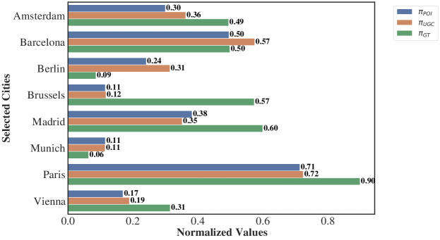
Figure 3. Bar plot showing the normalized values of the popularity index components for selected cities

4.2. Estimating Destination Popularity

Quantifying a city’s popularity is complex due to its multifaceted nature. In this paper, we propose a method to define city popularity based on metrics derived from Tripadvisor and the GT data as explained above in Section 4.1. The popularity index $\rho(c_{i})$ of a city $\mathit{c_{i}}$ is expressed as a weighted sum of various popularity components —- $\pi_{POI}$, $\pi_{UGC}$, and $\pi_{GT}$ denoting the points of interest, number of reviews and opinions available on Tripadvisor and google trends index for the last one year respectively for a city $\mathit{c_{i}}$. To ensure consistency, we employ min-max normalization (Patro and Sahu, 2015), as depicted in Equation 2, to standardize all component values within the range of 0 to 1.  Figure 3 displays the normalized values of various components constituting the popularity index for a chosen group of cities. The contrast in popularity is evident, with larger cities like Paris and Barcelona grappling with overtourism, while Munich and Berlin, comparatively less popular, showcase a distinct difference. Based on this, we define the popularity index $\rho(c_{i})$ for the city $\mathit{c_{i}}$ as follows:

(3) $$\rho(c_{i})=\beta_{POI}\cdot\pi_{POI}+\beta_{UGC}\cdot\pi_{UGC}+\beta_{GT}\cdot\pi_{GT}$$

Where $\beta_{j}$ for $j\in\{POI,UGC,GT\}$ are the weights assigned to each component of the popularity index. We derive the weights, $\beta_{j}$, for the popularity index components through a user study, as detailed in Section 6. This process involves determining the quantitative contributions of factors within the popularity elements to the overall popularity index, relying on user preferences and perceptions. By adopting this user-driven approach, the assigned weights for each component reflect user opinions and behaviors, thereby incorporating a human-centered dimension into the calculation of city popularity.

We aim to recommend destinations with a lower popularity index $\rho(c_{i})$, fostering a balanced distribution of tourist traffic, even in less popular yet attractive places. This approach seeks to mitigate the issue of overtourism at popular destinations.

5. Seasonal Destination Demand

The personalized recommendation algorithms in online platforms frequently highlight certain destinations, resulting in seasonal concentration of tourists. This pattern of recommendation can inadvertently lead to less-visited destinations remaining unnoticed. Consequently, the information presented online tends to direct visitors to these highlighted destinations, particularly in peak seasons, which can lead to temporary but significant increases in visitor numbers during specific times of the year (Gowreesunkar and Vo Thanh, 2020). TRS can intervene in this issue by redirecting tourists to less crowded destinations and avoiding peak seasons, thereby ensuring a consistent distribution of tourists throughout the year across all seasons.

Without specific data on destination demand, we employ city seasonality metrics as a proxy measure to assess its popularity among tourists at different times throughout the year. Cities can exhibit diverse patterns, with some having a singular peak, others featuring two peaks, and some maintaining a steady stream of tourists year-round (Butler, 1998; Corluka, 2019).

When considering the causes of seasonality in tourism, literature primarily distinguishes between natural and institutional causes. Natural causes are predominantly related to climatic conditions and are particularly evident in certain forms of tourism, such as summer vacation tourism. However, for example, health and business tourism tend to be more resistant to the natural causes of seasonality. Institutional causes are linked to written and non-written norms and customs that dictate social practices, including school holidays, state holidays, or specific festivities (Suštar and Ažić, 2020).

Our objective is to attribute a seasonal demand index to each city for a given month, providing an estimation of its appeal to tourists. The aim is to recommend destinations with lower seasonality indices, ensuring a consistent tourist presence throughout the year or balancing tourist loads across different destinations. As illustrated in Figure 1, the user interface provides recommendations tailored to a chosen time frame, such as a particular month. However, it’s important to differentiate between the data used for these recommendations: while the popularity index offers an aggregated view of a destination’s appeal over the entire year, the seasonality index, on the other hand, provides a more nuanced, month-by-month analysis. This distinction is essential for travelers planning their trips. The popularity index, although helpful, might not fully capture the unique characteristics or visitor trends of a destination in a specific month. In contrast, the seasonality index, with its monthly granularity, offers a more accurate representation of what a traveler can expect during their chosen travel period.

5.1. Data Gathering

To gauge the seasonal variations in tourist activity, we explore monthly visitor counts and bednight statistics from TourMIS and financial seasonality indicators, such as the average daily rates (ADR) from Airbnb. The ensuing sections elaborate on these data-gathering processes.

Table 3. Table summarizing different data sources and their basic statistics for calculating the destination’s seasonality index

Data Source	Attributes		Statistics
			# Cities	Min	Mean	SD	Max
TourMIS	NFIs	AVC	64	489	192,125.56	293,783.60	2,188,497
		BN	69	1,163	415,708.25	675,550.57	5,260,073
Airbnb	FI	ADR	45	68.09	316.88	418.63	2013.13

5.1.1. TourMIS

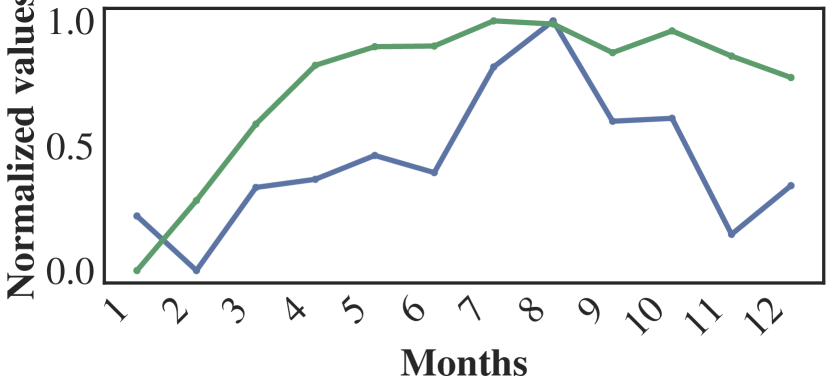
(a) Amsterdam

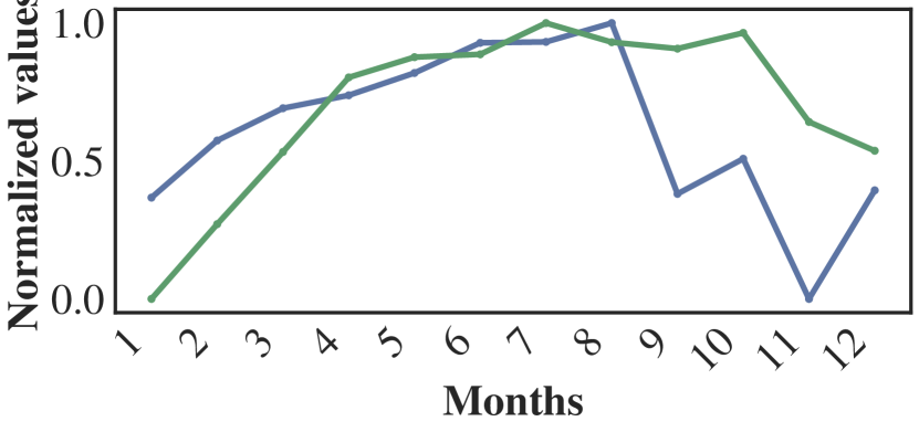
(b) Barcelona

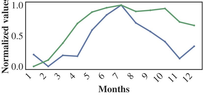
(c) Berlin

(d) Brussels

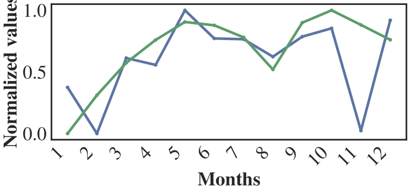
(e) Madrid

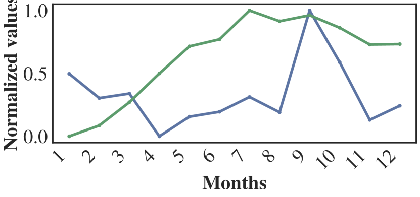
(f) Munich

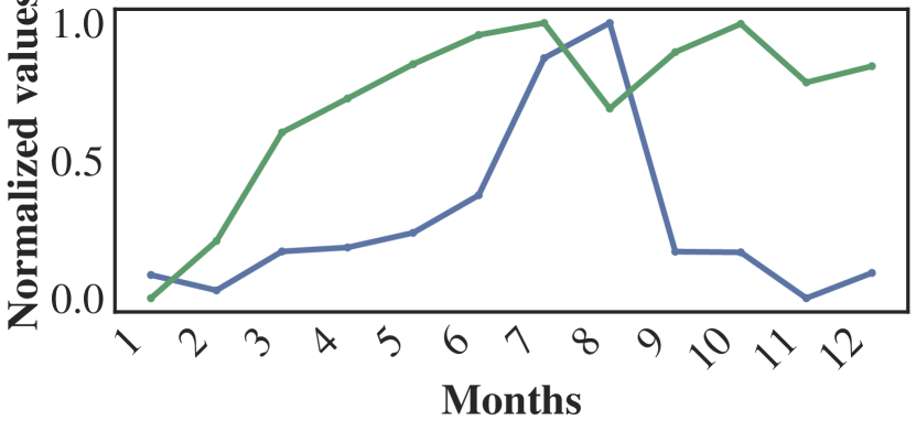
(g) Paris

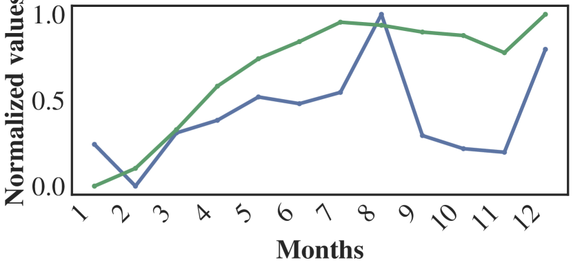
(h) Vienna

Figure 4. Visualization of the normalized monthly arrival visitor count (AVC) represented in green and monthly average listing price on Airbnb in blue for selected cities

TourMIS , a tourism marketing information system, offers complimentary and electronically accessible market research data to aid management decisions. Supported by the regional, national, and international tourist industry, TourMIS provides up-to-date tourism statistics and analyses, including arrivals and bed nights, for informed decision-making (Wöber, 2003). The monthly arrival visitor count (AVC), encompassing both foreign and domestic data, and the number of bed nights (BN) for European cities in 2022 are considered in our analysis. The dataset includes information for 65 cities regarding AVC and 70 cities for BN, with an overlap of 63 cities. Leveraging this data, we estimate the footfall in cities for respective months.

Exploratory data analyses on the TourMIS data revealed that a minimum AVC of 489.0 was recorded in January for the city of Eisenstadt, while Paris recorded a maximum AVC of 2,188,497 in July as evident from Table 3. Similarly, Eisenstadt, Austria documented the minimal number of bednights for January, while Paris still accounted for the maximum number in July. These insights illuminate the dynamic nature of tourism, showcasing the fluctuating visitor counts and bednights across various months and cities. Notably, the data suggests heightened touristic activity during the summer compared to winter.

We performed correlation analyses on the bednights (BN) and monthly AVC data from TourMIS. The results unveiled a consistently strong correlation (¿0.98) for each month among cities where data for both variables were available. To determine if this correlation trend holds for the entire population of cities, we carried out a T-Test (Eisenhart, 1979) with a significance level (p) of 0.05. The test yielded significant results, indicating sufficient evidence to conclude that the correlation significantly differs from zero in the population. Therefore, for our subsequent calculations, we exclusively consider the AVC numbers. It’s important to acknowledge that our approach utilizes absolute figures for AVC without normalizing them by the sizes of the cities. Although attempts were made to normalize for city sizes, the outcomes were heavily skewed towards small cities. We believe that our method accurately reflects the seasonal demands of smaller cities, which often feature numerous attractions.

5.1.2. Airbnb

To quantify the impact of financial indicators like average daily rate (ADR) on seasonality, we leverage the calendar.csv dataset sourced from Inside Airbnb . This dataset includes details on the availability and daily pricing of all listed accommodations within a city. Our analysis focuses on the latest data from September 2023 and covers a one-year duration for 45 European cities.

A foundational exploratory analysis of the data is presented in Table 3. In February, the lowest ADR was observed in Riga, while Oslo reported the highest ADR in July. These findings affirm the presence of seasonal demand variations across months, with increased demand in the summer, and align with the economic disparities between the cities (Statista Research Department, 2023a).  Figure 4 illustrates the normalized monthly AVC in green and the monthly average listing price on Airbnb in blue for selected cities. A positive correlation is observed between the two in most cases, except for Brussels. Specific peaks in Munich’s accommodation prices during October are representative of Oktoberfest, while generally, prices are elevated in the summer months, followed by a gradual decline in the winter months. Additionally, we applied standard correlation metrics to analyze the relationship between AVC and the average price of Airbnb listings for each city every month. The results consistently show a positive correlation for most cities except Brussels. This deviation in Brussels can be attributed to more business travelers (Santos and Cincera, 2018).

Despite these observed correlations, the correlation coefficients for each month across all cities were negatively correlated and statistically insignificant. Consequently, we opted to include the Average Daily Rate (ADR) values of the cities for each month as a separate component in our analysis of the financial indicators of tourism demand.

5.2. Estimating Seasonal Demand

In literature, the Gini coefficient stands out as a widely employed tool for assessing tourism seasonality (Þórhallsdóttir and Ólafsson, 2017; Suštar and Ažić, 2020; Ferrante et al., 2018). This coefficient offers distinct advantages, including its ability to consider distribution asymmetry, relative insensitivity to extreme values, and an indication of stability in the distribution of overnight stays within a single year (Suštar and Ažić, 2020). In our paper, the Gini coefficient serves as a numerical metric quantifying the level of inequality in the distribution (Gini, 1921). Derived from the Lorenz curve, which illustrates the cumulative frequency of ranked observations starting from the lowest number (Gastwirth, 1972), the Gini coefficient provides a comprehensive measure for the demand of the destination at a particular time of the year. The analytical formula frequently used for Gini coefficient calculation, applied in this paper, is expressed as (Gastwirth, 1972; Þórhallsdóttir and Ólafsson, 2017):

(4) $$G=\frac{2}{n}\sum_{i=1}^{n}(x_{i}-y_{i})$$

where

$$\begin{split}&n=\text{the number of fractiles, months, weeks, days, or other units}\\ &x_{i}=\text{the rank of fractiles, for example, }\\ &\quad\frac{1}{12},\frac{2}{12},\ldots\text{ when using months, or when using weeks }\\ &\quad\frac{1}{52},\frac{2}{52},\ldots,\text{ or days }\frac{1}{365},\frac{2}{365},\ldots,\text{ etc. So }x_{i}=\frac{i}{n}\\ &y_{i}=\text{the cumulated fractiles in the Lorenz curve}\\ \end{split}$$

In the context of seasonal tourism demand, studies suggest that the average room price is one of the pivotal business performance indicators in the hotel industry (Israeli, 2002; O’Neill and Carlbäck, 2011; Pine and Phillips, 2005). We calculate the seasonality Gini index for a city using Gini Coefficients derived from non-financial and financial indicators, as described by Suštar and Ažić (2020). Non-financial indicators consist of monthly counts of arriving visitors (AVC) from TourMIS, while financial indicators involve the Average Daily Rate (ADR) computed from Airbnb listings. The Gini coefficient values for each indicator span from zero to one, with zero signifying a complete lack of seasonality and seems to be an active or equal distribution of volumes all year round, and a Gini coefficient of one indicates complete seasonality, i.e., the total volume is registered in one single month (Suštar and Ažić, 2020). Gini coefficients are computed annually for AVC, while monthly calculations are performed for ADR.

As illustrated in  Figure 4, the monthly average prices of listings exhibit significant fluctuations depending on the city and month. Therefore, it is advisable to model these fluctuations daily to enhance the precision of our estimations. Similarly, if data is available daily or weekly granularity, the AVC numbers could be modeled at those levels for more accurate analyses. The aggregated seasonality index $\sigma(c_{i}^{j})$  across all indicators for a city $c\_{i}$ for month $j$ for can be calculated as follows:

(5) $$\sigma(c_{i}^{j})=\Gamma_{AVC}\cdot G_{AVC}^{(i)}+\Gamma_{ADR}\cdot G_{ADR}^{(i)(j)}$$

Where $\Gamma_{k}$ where $k\in\{AVC,ADR\}$ represents the weights as derived from the user study. We aim to recommend cities with lower $\sigma(c_{i}^{j})$, ensuring a consistent tourist presence throughout the year or balancing tourist loads across different destinations.

From a selected list of cities common in all datasets, we calculate the Gini coefficients for the AVC and ADR, presenting the results in Table 4. Madrid exhibits the least seasonality in AVC, suggesting consistent demand throughout the year, while Munich registers the highest seasonality. Additionally, Brussels displays minimal seasonality in ADR (close to 0), and Munich exhibits maximum ADR seasonality in September and October. The heightened seasonality in Munich’s AVC and ADR can also be attributed to the annual Oktoberfest event occurring in September (Herrmann and Herrmann, 2014).

Table 4. Gini coefficients illustrating the seasonality indicators in selected citiesThe bold notations highlight the maximum Gini indices for ADR in the city, while the italicized and underlined ones denote the minimum

City	$G_{AVC}$	$G_{ADR}$
		Jan	Feb	Mar	Apr	May	Jun	July	Aug	Sep	Oct	Nov	Dec
Amsterdam	0.146	0.033	0.010	0.019	0.017	0.014	0.011	0.044	0.014	0.063	0.060	0.026	0.047
Barcelona	0.115	0.040	0.108	0.051	0.027	0.026	0.026	0.008	0.025	0.029	0.025	0.026	0.097
Berlin	0.158	0.028	0.019	0.020	0.015	0.026	0.051	0.046	0.026	0.040	0.022	0.018	0.056
Brussels	0.116	0.023	0.015	0.020	0.025	0.008	0.009	0.006	0.008	0.081	0.046	0.028	0.064
Madrid	0.079	0.037	0.024	0.041	0.028	0.045	0.028	0.025	0.020	0.059	0.055	0.037	0.073
Munich	0.188	0.013	0.008	0.029	0.010	0.020	0.036	0.033	0.032	0.138	0.049	0.009	0.033
Paris	0.100	0.017	0.007	0.012	0.008	0.013	0.009	0.139	0.150	0.078	0.039	0.013	0.044
Vienna	0.184	0.058	0.016	0.032	0.020	0.024	0.021	0.015	0.101	0.062	0.031	0.027	0.101

6. User Perception of Sustainable City Trips

To explore how the users perceive sustainability when looking for city trip recommendations, we conducted an inclusive user study involving participants with diverse travel experiences and preferences. This method was selected as a key approach to unravel the intricacies of decision-making, providing valuable insights into various facets of the process, as established by prior research (Wilson, 1981). By directly engaging real-world participants in simulated scenarios, our aim was to discern how tourists assess different aspects of a city trip, negotiate trade-offs, align preferences with sustainable tourism practices, and assign weights to criteria in their decision-making.

6.1. User Study Design

The primary objective of our user study was to gain a deeper understanding of the factors influencing individuals’ decisions when selecting a city for vacation and their receptiveness to sustainable recommendations for tourism destinations. Respondents were prompted to imagine planning their next vacation to another European city and identify the most crucial factors influencing their choice of destination. Only a limited set of personal demographic questions pertaining to the users’ age, gender, and nationality were asked to preserve the participants’ privacy.

The questionnaire was designed using Qualtrics Experience Management Software , an online survey platform. We recruited participants through the online crowdsourcing platform Prolific , renowned for its efficacy in subject recruitment for the scientific community (Palan and Schitter, 2018). With a focus on European participants who listed travel as one of their hobbies, the questionnaire, designed in English, was distributed to 200 individuals through Prolific’s advanced pre-screening options. To ensure gender diversity, the preset distribution aimed for an equal representation of 50% males and 50% females. Demographic analyses of the survey data indicated that 33.8% of the participants fell within the 25-34 age group, followed by 24.3% in the 18-24 age group, and the remaining were above the age of 35.

6.2. Transportation Sustainability Concerns

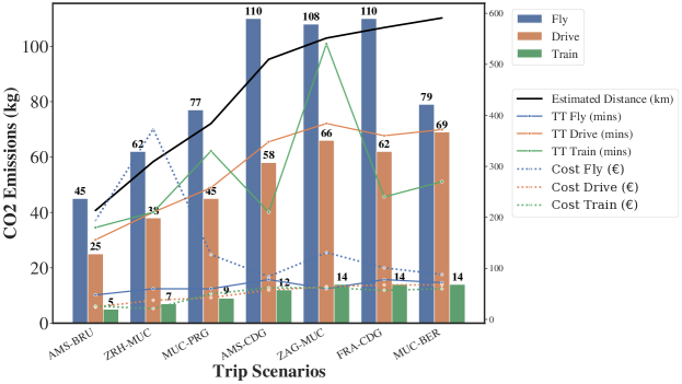
Figure 5. CO₂e, travel time (TT), estimated distance, and cost as shown to the users for each trip scenario, separated by transportation mode. Each city in every trip scenario is denoted by its respective IATA code

Participants were presented with seven distinct scenarios, elaborated in Figure 5. These scenarios illustrated trips between cities involving diverse modes of transportation—–such as train, flight, and driving with the intention of gauging their inclination towards making sustainable choices when selecting their mode of transport. We estimated costs associated with one-way nonstop flight and train connections up to a maximum distance of 500 kilometers using the estimations from Rome2Rio (2018), projected for approximately one month in advance. We approximated the cost of driving based on the estimates from European Commission – Alternative Fuels Observatory (2022) for a petrol car. The CO₂e estimations, tailored to each mode of transportation, were computed based on the values in Table 1.

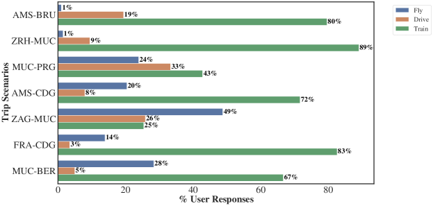
Figure 6. Distribution of user responses (%) for different transport modes in various trip scenarios. Each city in every trip scenario is denoted by its respective IATA code

Figure 6 provides a summary of the mode distribution for various city pairs, indicating the percentages of user responses for different transportation modes (train, drive, and fly). Key takeaways include preferences for specific modes for each trip, reflecting the distribution of travel choices considering the associated distances. Notably, train travel dominates in several instances, with variations depending on the city pairs and their distances. The percentages of user responses offer insights into the preferred transportation modes for different travel scenarios.

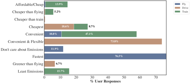
Figure 7. Reasonings provided by respondents when choosing modes of transport across all trips

We delved into the reasons behind selecting trade-offs for various transportation modes in each trip scenario, as illustrated in Figure 7. Our analysis reveals notable insights from survey responses. For train travel, a significant 47.1% of respondents prioritize convenience, while 15.65% emphasize selecting the mode with the least CO₂ emissions. Affordability is a critical factor for 13.91% of participants, and 8.70% opt for the cheapest option available. Additionally, 5.22% favor trains over flights for cost considerations. In contrast, driving is primarily chosen for its convenience and flexibility, with an overwhelming 73.81% of respondents highlighting this aspect. Affordability remains a factor, as 18.57% opt for the cheapest driving option. Some respondents (6.67%) perceive driving as environmentally better than flying. Flying, chosen by 76.53% for its speed, also reflects a segment (11.91%) indifferent to CO₂ emissions. The findings underline the multifaceted nature of decision-making, encompassing convenience, environmental concerns, and cost considerations across different transportation modes. These findings align with the outcomes presented by Avogadro et al. (2021). They similarly indicate a preference for public transport over flying for shorter distances.

6.3. Understanding Tradeoffs

The user study also aimed to explore the various trade-offs associated with trip planning. Participants were presented with Likert Scale (Joshi et al., 2015) statements from ”not at all important” to ”extremely important” to gauge their agreement levels to the following statements:

• Importance of presence of off-season discounts.

• Climate at the destination.

• Cost savings by traveling during off-season.

• Visiting the city during its best travel time, even during the peak tourist season.

• Overall attractiveness of the destination.

• The destination in terms of unique attractions, points of interest, etc., even if that means they are very popular.

• Cities that are widely popular, even if they might be crowded.

The analysis of user responses, as depicted in Figure 8, provides insights into the trade-offs users are willing to make when considering various attributes in travel decision-making. Notably, for the attribute ”popular but crowded,” a minimal percentage (2.99%) strongly agreed, while the majority (31.34%) agreed. Conversely, for the attribute ”attractive but popular”, a significant proportion (55.22%) agreed, indicating a higher tolerance for popularity in the pursuit of attractiveness. The consideration of ”overall attractiveness” saw 51.24% in agreement. Respondents expressed varying opinions on the ”visiting in peak season”, with 1.99% strongly disagreeing and 33.83% expressing disagreement. Furthermore, factors such as ”off-season cost savings”, ”Climate at the destination” during the time of travel, and ”off-season discounts” revealed nuanced preferences, with notable percentages in agreement (51.74%, 37.31%, 39.30%, respectively) and distinct proportions holding dissenting views. These results contribute valuable insights into the multifaceted considerations influencing users’ travel preferences.

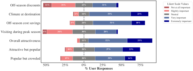
Figure 8. Figure showing the degree of importance of the various factors during a trip decision-making process

7. Societal Fairness

This section delves into quantifying S-Fairness, a pivotal element in examining city trip recommendations. Societal Fairness (S-Fairness) involves ensuring the fair distribution of tourism benefits and impacts among a spectrum of stakeholders, encompassing not only travelers, item providers, and platforms but also non-participating entities such as residents, locals, and the environment (Banerjee, 2023; Banik et al., 2023).

To assess Societal Fairness (S-Fairness) across diverse destinations, our methodology integrates insights from established data sources and incorporates findings from an extensive user study, providing a thorough perspective. We define the S-Fairness index (SF index) by quantifying the overall impact of a destination on both the environment and society concerning the user’s starting point.

7.1. Defining the S-Fairness Index

Each destination $\mathit{c_{i}}$ during the month $j$ accessible from the user’s origin is assigned an SF index, denoted as $\psi(c_{i}^{j})$. This index is determined through a weighted combination of three essential indicators—

• emissions trade-off indicator $\mathit{Z(c_{i})}$ from Section 3 with its normalized weight represented by $\alpha$

• popularity index $\rho(c_{i})$ from Section 4 with its normalized weight denoted as $\beta$

• seasonality index $\sigma(c_{i}^{j})$ from Section 5 with its normalized weight represented by $\Gamma$.

The formulation is expressed as:

(6) $$\psi(c_{i}^{j})=\alpha\cdot Z(c_{i})+\beta\cdot\rho(c_{i})+\Gamma\cdot\sigma(c_{i}^{j})$$

Here, $\psi(c_{i}^{j})$ falls within the range of zero to one, where a higher index signifies a more adverse impact on society. The allocation of weights to these indicators reflects the significance of considering emissions, popularity, and seasonality in evaluating the societal fairness of a destination. This approach, integrating both quantitative and user-centered perspectives, strengthens the effectiveness of our S-Fairness indicator.

7.2. Learning Weights of the Indicators

Here, we aim to gauge the respondents’ perceived importance of various factors influencing their selection of travel destinations. In the user study described in Section 6.1, the participants were also prompted to allocate maximum weightage among travel time, CO₂ footprint, and cost when determining transportation to their destination, aligning with the coefficients outlined in the calculation of the emissions trade-off indicator $\mathit{Z(c_{i})}$ in  Equation 1. They also provided insights into the significance of factors like points of interest counts, Google image search values, and the total number of Tripadvisor reviews and opinions, detailed in the estimation of the popularity index $\rho(c_{i})$ in Equation 3, to determine the popularity of a city. They also indicated the importance of costs associated with available accommodation and crowd levels in the city during their visit, aligning with the coefficients of the seasonality index in Equation 5. This aimed to shed light on the impact of seasonality on the decision-making process.

Finally, the participants were prompted to assess the influence of various factors on their decision-making process to estimate the weights associated with the combined S-Fairness index $\psi(c_{i}^{j})$, as illustrated in Equation 6. They were explicitly asked about the impact of factors such as having a lower CO₂ footprint, opting for a less famous city, and avoiding the busiest time of the year when making travel decisions. All the responses were gathered using a 5-point Likert Scale.

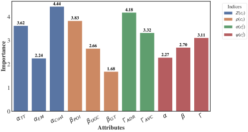
Figure 9. Distribution of the absolute values of weights, obtained through the weighted average of Likert scale results

We calculated weighted averages on Likert scales, spanning from ”not important at all”, having a minimum weight of 1, to ”extremely important”, with a maximum weight of 5, enabling us to identify patterns in the composite scores. The Distribution of the absolute values of these weights, obtained through the weighted average of Likert scale results, are shown in  Figure 9. Additionally, we applied min-max normalization (Patro and Sahu, 2015) to normalize these averages within each category, enabling us to gauge their relative significance in their respective categories. These normalized weights offer valuable insights into participants’ preferences and priorities, shedding light on the factors that significantly influence their decision-making when choosing travel destinations. After incorporating the normalized weights, the expressions for the emissions trade-off indicator, popularity index, and seasonality index can be revised as follows:

(7) $$\mathit{Z(c_{i})}=0.352\cdot\tau_{TT}({\mathit{c_{i}}})+0.218\cdot\tau_{EM}({\mathit{c_{i}}})+0.431\cdot\tau_{Cost}({\mathit{c_{i}}})$$

(8) $$\rho(c_{i})=0.469\cdot\pi_{POI}+0.325\cdot\pi_{UGC}+0.206\cdot\pi_{GT}$$

(9) $$\sigma(c_{i}^{j})=0.443\cdot G_{AVC}^{(i)}+0.557\cdot G_{ADR}^{(i)(j)}$$

Combining the weighted formulations presented in Equation 7, Equation 8, and Equation 9, we obtain the updated values for the S-Fairness index $\psi(c_{i}^{j})$ as follows:

(10) $$\psi(c_{i}^{j})=0.281\cdot\mathit{Z(c_{i})}+0.334\cdot\rho(c_{i})+0.385\cdot\sigma(c_{i}^{j})$$

The weights here represent the importance assigned to different attributes within each category. Notably, in the emission trade-off category $\mathit{Z(c_{i})}$, the highest weight is given to the cost attribute ($\alpha_{Cost}$), indicating that users prioritize the cost factor when evaluating emission scores. In the popularity category $\rho(c_{i})$, the points of interest ($\beta_{POI}$) attribute carries the highest weight, suggesting that users prioritize locations with significant points of interest. However, in the S-Fairness index category $\psi(c_{i}^{j})$, the weight distribution is relatively balanced among the attributes $\alpha$, $\beta$, and $\Gamma$, indicating a more equitable consideration of these factors. These weights provide insights into user preferences, highlighting the relative importance of different attributes within each category. The normalized weights further emphasize the relative significance of characteristics within their respective categories, aiding in understanding user priorities and preferences in decision-making.

Figure 10 shows the distribution of the weighted seasonality indices for selected cities. It captures the pronounced peaks in monthly seasonality for Munich in September and Paris in July/August as shown in Table 4. We did not plot the weighted popularity scores as they were similar to the results in Figure 3.

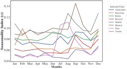
Figure 10. Distribution of the weighted seasonality index for selected cities

The composite S-Fairness index $\psi(c_{i}^{j})$ assigned to each city $\mathit{c_{i}}$ for the month $j$ signifies the extent of negative environmental impact associated with traveling to the city from users’ starting points. A lower value of $\psi(c_{i}^{j})$ indicates a more environmentally friendly choice and lesser harm caused. Our objective is to encourage individuals to visit cities with lower S-Fairness indices relative to their starting points, aiming to minimize the adverse effects of tourism on the environment and promote sustainable and responsible tourism practices.

7.3. Validating S-Fairness Index

The validation of the S-Fairness index is a pivotal part of our study. Here, we detail the process undertaken for this validation, highlighting how the index performs in real-world scenarios and reflects a balance between tourist preferences and sustainable practices.

To evaluate the effectiveness of our SF indices, we conducted a user study involving a gender-balanced sample of 200 European residents with a listed interest in travel on Prolific. Participants were presented with the Figure 1 from Section 1, featuring the top travel destinations from Munich for July. The study showcased six European cities, each accompanied by a photograph and a brief overview. Featured cities include Vienna, Berlin, Brussels, Madrid, Barcelona, and Paris. Each destination is accompanied by travel time information by train and plane from Munich, carbon emissions for each mode of transport, and three indices, Emission, Popularity, and Seasonality, with qualitative ratings such as ”Medium” or ”High” for trade-off understanding. In this scenario, cities within the top 5 percentile of their respective popularity and seasonality indices are categorized as high, those in the top 50 percentile as medium, and the rest as low.

An overall SF index out of 100 is assigned to each city (derived by multiplying our SF index from Section 7.2 by 100), representing its overall sustainability status concerning the starting point, Munich. Vienna and Berlin score 19/100, being the most sustainable options from Munich, followed by Brussels 22/100. Madrid 30/100, Barcelona 33/100, and Paris 39/100 are the least sustainable options at the end of the list. The interface aims to assist users in choosing a travel destination based on sustainability, popularity metrics, and personal interest. The presented SF indices indicate the preference for sustainable destinations. Through the interface, users will also have the option to choose their preferred mode of transport, and the SF index value will be updated accordingly.

Following the presentation, participants were tasked with expressing their opinions on the provided statements using a 5-point Likert Scale (Joshi et al., 2015) ranging from ”strongly disagree” to ”strongly agree”. The statements covered the following aspects:

• The assigned SF index scores accurately reflect the sustainability of the showcased city destinations.

• Cities with lower SF index scores are perceived as more appealing for travel.

• SF indices are deemed helpful in facilitating informed decisions about preferred travel destinations.

The results are depicted in Figure 11, revealing a generally positive reception to the SF index as a sustainability indicator. A majority of users (72%) expressed neutrality or agreement. The ”low SF index, better appeal” metric showed a similar trend, with 71% ranging from neutral to solid agreement, suggesting that a lower SF index correlates with higher user appeal. The ”overall helpful metric” received the most positive responses, with 77.5% ranging from neutral to solid agreement on its usefulness. Overall, there is a trend of approval across all metrics, with even the least favorable response showing a majority of users being neutral to strongly agreeing on the value of the metrics. In conclusion, the metrics presented in the study are well-received by most users.

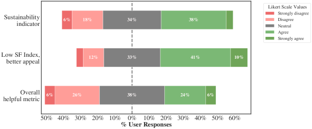
Figure 11. Results of the user study to validate the usefulness of the SF index, showing a mostly positive response

8. Conclusion

In conclusion, our research introduces a novel approach for assigning a sustainability indicator (SF index) for city trips accessible from the users’ starting point, integrating CO₂ emission analysis, destination popularity, and seasonal demand. Our methodology, validated through a user study, showcases the practicality and effectiveness of the model in providing well-rounded and sustainable city trip suggestions. Our findings indicate that while there is a general awareness of sustainability, tourists often prioritize convenience and personal preferences over sustainable choices. This gap highlights the need for more effective communication and education strategies to promote S-Fairness in city trip planning.

This work lays the groundwork for significant enhancements in TRS. While Figure 1 serves as an illustrative user interface, the potential of this work extends to the development of a practical application. Such an application could present destinations and their SF indices, incorporating up to date information like real-time connectivity and cost considerations. Moreover, it could integrate additional metrics such as accommodation availability and environmental factors like climate and air quality indices. This integration, coupled with user preferences, would enable the provision of real-time recommendations that align with sustainability principles and individual user preferences.

Additionally, as depicted in Figure 1, destinations are currently ordered by the SF index. However, in practical scenarios, users may prefer sorting destinations by factors such as emissions, popularity, and seasonality, given their varying importance to different individuals. Introducing a user interface that allows sorting and filtering by the individual components while making the associated trade-offs explicit would enhance the flexibility of the application. Similarly, the current representation of popularity and seasonality labels (e.g., low, medium, or high) in Figure 1 could be refined through discrete categories to offer meaningful and actionable insights, contributing to a more user-friendly and informative interface. We intend to delve deeper into the communication of sustainable recommendations to users as part of our future research.

In summary, our study marks an essential stride towards a new era in sustainable tourism. It paves the way for a system that combines environmentally sensitive travel suggestions with travelers’ evolving needs and preferences.

References

- (1)
- Abdollahpouri et al. (2020) Himan Abdollahpouri, Gediminas Adomavicius, Robin Burke, Ido Guy, Dietmar Jannach, Toshihiro Kamishima, Jan Krasnodebski, and Luiz Pizzato. 2020. Multistakeholder recommendation: Survey and research directions. User Modeling and User-Adapted Interaction 30, 1 (2020), 127–158. https://doi.org/10.1007/s11257-019-09256-1
- Abdollahpouri and Burke (2021) Himan Abdollahpouri and Robin Burke. 2021. Multistakeholder recommender systems. In Recommender systems handbook. Springer, 647–677. https://doi.org/10.1007/978-1-0716-2197-4_17
- Avogadro et al. (2021) Nicolò Avogadro, Mattia Cattaneo, Stefano Paleari, and Renato Redondi. 2021. Replacing short-medium haul intra-European flights with high-speed rail: Impact on CO2 emissions and regional accessibility. Transport Policy 114 (2021), 25–39. https://doi.org/10.1016/j.tranpol.2021.08.014
- Aziz and Ukkusuri (2014) HM Abdul Aziz and Satish V Ukkusuri. 2014. Exploring the trade-off between greenhouse gas emissions and travel time in daily travel decisions: Route and departure time choices. Transportation Research Part D: Transport and Environment 32 (2014), 334–353. https://doi.org/10.1016/j.trd.2014.07.016
- Balakrishnan and Wörndl (2021) Gokulakrishnan Balakrishnan and Wolfgang Wörndl. 2021. Multistakeholder Recommender Systems in Tourism. Proc. Workshop on Recommenders in Tourism (RecTour 2021) (2021).
- Banerjee (2023) Ashmi Banerjee. 2023. Fairness and Sustainability in Multistakeholder Tourism Recommender Systems. In Proceedings of the 31st ACM Conference on User Modeling, Adaptation and Personalization (Limassol, Cyprus) (UMAP ’23). ACM, New York, NY, USA, 274–279. https://doi.org/10.1145/3565472.3595607
- Banerjee et al. (2023) Ashmi Banerjee, Paromita Banik, and Wolfgang Wörndl. 2023. A review on individual and multistakeholder fairness in tourism recommender systems. Frontiers in big Data 6 (2023), 1168692. https://doi.org/10.3389/fdata.2023.1168692
- Banik et al. (2023) Paromita Banik, Ashmi Banerjee, and Wolfgang Wörndl. 2023. Understanding User Perspectives on Sustainability and Fairness in Tourism Recommender Systems. In UMAP’23 Adjunct: Adjunct Proceedings of the 31st ACM Conference on User Modeling, Adaptation and Personalization (UMAP ’23) (Limassol, Cyprus). ACM, New York, NY, USA, 8. https://doi.org/10.1145/3563359.3597442
- Beirman (2020) David Beirman. 2020. Restoring tourism destinations in crisis: A strategic marketing approach. Routledge.
- Brander and Davis (2012) Matthew Brander and Gary Davis. 2012. Greenhouse gases, CO2, CO2e, and carbon: What do all these terms mean. Econometrica, White Papers (2012).
- Butler (1998) Richard Butler. 1998. Seasonality in tourism: Issues and implications. The Tourist Review 53, 3 (1998), 18–24. https://doi.org/10.1108/eb058278
- Camarda and Grassini (2003) D Camarda and L Grassini. 2003. Environmental impacts of tourism. Conference on the Relationships between Global Trades and Local Resources in the Mediterranean Region, 2002/04, Rabat (Morocco) (2003), 263–270.
- Carbon Independent (2023) Carbon Independent. 2023. Carbon Independent - Reducing your carbon footprint. https://www.carbonindependent.org/22.html
- Cernat and Gourdon (2012) Lucian Cernat and Julien Gourdon. 2012. Paths to success: Benchmarking cross-country sustainable tourism. Tourism Management 33, 5 (Oct. 2012), 1044–1056. https://doi.org/10.1016/j.tourman.2011.12.007
- Clasen (2020) Thies Clasen. 2020. Bahn Expert. https://bahn.expert/
- Corluka (2019) Goran Corluka. 2019. Tourism seasonality–an overview. Journal of Business Paradigms 4, 1 (2019), 21–43.
- Dadoun et al. (2019) Amine Dadoun, Raphaël Troncy, Olivier Ratier, and Riccardo Petitti. 2019. Location Embeddings for Next Trip Recommendation. In Companion Proceedings of The 2019 World Wide Web Conference (WWW ’19). ACM. https://doi.org/10.1145/3308560.3316535
- Dastgerdi and De Luca (2023) Ahmadreza Shirvani Dastgerdi and Giuseppe De Luca. 2023. A post-pandemic look at short-term tourist accommodations and World Heritage Site management. Journal of Tourism and Cultural Change (2023), 1–12. https://doi.org/10.1080/14766825.2022.2164502
- DEFRA (2007) DEFRA. 2007. Act on CO2 Calculator: Public Trial Version Data, Methodology and Assumptions Paper. http://www.defra.gov.uk/environment/climatechange/uk/individual/pdf/actonco2-calc-methodology.pdf
- Dodds and Butler (2019) Rachel Dodds and Richard Butler. 2019. The phenomena of overtourism: A review. International Journal of Tourism Cities 5, 4 (2019), 519–528. https://doi.org/10.1108/IJTC-06-2019-0090
- Eisenhart (1979) Churchill Eisenhart. 1979. On the transition from” Student’s” z to” Student’s” t. American Statistician (1979), 6–10. https://doi.org/10.1080/00031305.1979.10482643
- Euronews (2023) Euronews. 2023. Rail Fares Across Europe: The Countries with the Most Expensive Train Tickets. https://www.euronews.com/travel/2023/01/09/rail-fares-across-europe-the-countries-with-the-most-expensive-train-tickets
- European Commission – Alternative Fuels Observatory (2022) European Commission – Alternative Fuels Observatory. 2022. Fuel Price Comparison. https://alternative-fuels-observatory.ec.europa.eu/consumer-portal/fuel-price-comparison
- Fernández and Rivero (2009) Juan Ignacio Pulido Fernández and Marcelino Sánchez Rivero. 2009. Measuring tourism sustainability: proposal for a composite index. Tourism Economics 15, 2 (2009), 277–296. https://doi.org/10.5367/000000009788254377
- Ferrante et al. (2018) Mauro Ferrante, Giovanni L Lo Magno, and Stefano De Cantis. 2018. Measuring tourism seasonality across European countries. Tourism Management 68 (2018), 220–235. https://doi.org/10.1016/j.tourman.2018.03.015
- Galí (2022) Núria Galí. 2022. Impacts of COVID-19 on local tour guides. Journal of Tourism and Cultural Change 20, 6 (2022), 788–805. https://doi.org/10.1080/14766825.2022.2046016
- Gastwirth (1972) Joseph L Gastwirth. 1972. The estimation of the Lorenz curve and Gini index. The review of economics and statistics (1972), 306–316. https://doi.org/10.2307/1937992
- Ghosh et al. (2020) RK Ghosh, Arnab Bhattacharyya, et al. 2020. Eco-Routing Using Open Street Maps. arXiv preprint arXiv:2011.13556 (2020). https://doi.org/10.48550/arXiv.2011.13556
- Gini (1921) Corrado Gini. 1921. Measurement of inequality of incomes. The economic journal 31, 121 (1921), 124–125. https://doi.org/10.2307/2223319
- Google (2019) Google. 2019. Google Travel Impact Model. Google Developers. https://developers.google.com/travel/impact-model
- Gorantla and Bansal (2023) Ramesh Gorantla and Srividya Bansal. 2023. Towards a Sustainability Index Calculator for Smart Cities. In Companion Proceedings of the ACM Web Conference 2023. 715–722. https://doi.org/10.1145/3543873.3587683
- Gössling (2017) Stefan Gössling. 2017. Tourism, information technologies and sustainability: an exploratory review. Journal of Sustainable Tourism 25, 7 (2017), 1024–1041.
- Gowreesunkar and Vo Thanh (2020) Vanessa Gaitree Gowreesunkar and Tan Vo Thanh. 2020. Between overtourism and under-tourism: Impacts, implications, and probable solutions. Overtourism: Causes, implications and solutions (2020), 45–68. https://doi.org/10.1007/978-3-030-42458-9_4
- Graver et al. (2019) Brandon Graver, Kevin Zhang, and Dan Rutherford. 2019. Emissions from commercial aviation, 2018. In International Council on Clean Transportation. International Council on Clean Transportation.
- Herrmann and Herrmann (2014) Roland Herrmann and Oliver Herrmann. 2014. Hotel roomrates under the influence of a large event: The Oktoberfest in Munich 2012. International Journal of Hospitality Management 39 (2014), 21–28. https://doi.org/10.1016/j.ijhm.2014.01.006
- Herzog et al. (2019) Daniel Herzog, Sherjeel Sikander, and Wolfgang Wörndl. 2019. Integrating Route Attractiveness Attributes into Tourist Trip Recommendations. In Companion Proceedings of The 2019 World Wide Web Conference (WWW ’19). ACM. https://doi.org/10.1145/3308560.3317052
- Hilali and Belmaghraoui (2019) Miloudi Hilali and Walid Belmaghraoui. 2019. Contribution to the study of polluting emissions on the environment and anti-pollution standards in diesel and gasoline engines. Journal of Industrial Pollution Control (2019).
- Hoffmann et al. (2022) Felix J. Hoffmann, Fabian Braesemann, and Timm Teubner. 2022. Measuring sustainable tourism with online platform data. EPJ Data Science 11, 1 (July 2022). https://doi.org/10.1140/epjds/s13688-022-00354-6
- Ian Tiseo (2023) Ian Tiseo. 2023. Carbon footprint of travel per kilometer by mode of transport. https://www.statista.com/statistics/1185559/carbon-footprint-of-travel-per-kilometer-by-mode-of-transport/
- Iken and Aguessy (2022) N Iken and FX Aguessy. 2022. Calculating the Greenhouse Gas Emissions of Flights: A Comparative Study of Existing Protocols. In IOP Conference Series: Earth and Environmental Science, Vol. 952. IOP Publishing, 012002. https://doi.org/10.1088/1755-1315/952/1/012002
- Irem et al. (2017) Ã Irem, WÃ Karl, Bozana Zekan, et al. 2017. Towards a sustainable urban tourism development in Europe. Tourism Economics 23, 2 (2017), 243–259.
- Isinkaye et al. (2015) F.O. Isinkaye, Y.O. Folajimi, and B.A. Ojokoh. 2015. Recommendation systems: Principles, methods and evaluation. Egyptian Informatics Journal 16, 3 (2015), 261–273. https://doi.org/10.1016/j.eij.2015.06.005
- Israeli (2002) Aviad A Israeli. 2002. Star rating and corporate affiliation: their influence on room price and performance of hotels in Israel. International Journal of Hospitality Management 21, 4 (2002), 405–424. https://doi.org/10.1016/S0278-4319(02)00037-3
- Jannach and Bauer (2020) Dietmar Jannach and Christine Bauer. 2020. Escaping the McNamara Fallacy: Toward More Impactful Recommender Systems Research. Ai Magazine 41 (12 2020), 79–95. https://doi.org/10.1609/aimag.v41i4.5312
- Joshi et al. (2015) Ankur Joshi, Saket Kale, Satish Chandel, and D Kumar Pal. 2015. Likert scale: Explored and explained. British journal of applied science & technology 7, 4 (2015), 396–403.
- Ko (2005) Tae Gyou Ko. 2005. Development of a tourism sustainability assessment procedure: a conceptual approach. Tourism management 26, 3 (2005), 431–445. https://doi.org/10.1016/j.tourman.2003.12.003
- Larsson and Kamb (2022) Jörgen Larsson and Anneli Kamb. 2022. Methodology Report. Technical Report. Chalmers University of Technology and KTH Royal Institute of Technology. https://travelco2.com/met/methodology-report-travelco2.pdf
- Lashof and Ahuja (1990) Daniel A Lashof and Dilip R Ahuja. 1990. Relative contributions of greenhouse gas emissions to global warming. Nature 344, 6266 (1990), 529–531. https://doi.org/10.1038/344529a0
- Lim et al. (2015) Kwan Hui Lim, Jeffrey Chan, Christopher Leckie, and Shanika Karunasekera. 2015. Personalized tour recommendation based on user interests and points of interest visit durations. In Twenty-Fourth International Joint Conference on Artificial Intelligence.
- Liu et al. (2011) Qi Liu, Yong Ge, Zhongmou Li, Enhong Chen, and Hui Xiong. 2011. Personalized travel package recommendation. In 2011 IEEE 11th international conference on data mining. IEEE, 407–416. https://doi.org/10.1109/ICDM.2011.118
- Lu et al. (2012) Eric Hsueh-Chan Lu, Ching-Yu Chen, and Vincent S. Tseng. 2012. Personalized trip recommendation with multiple constraints by mining user check-in behaviors. In Proceedings of the 20th International Conference on Advances in Geographic Information Systems (SIGSPATIAL’12). ACM. https://doi.org/10.1145/2424321.2424349
- Massimo and Ricci (2019) David Massimo and Francesco Ricci. 2019. Clustering users’ pois visit trajectories for next-poi recommendation. In Information and Communication Technologies in Tourism 2019: Proceedings of the International Conference in Nicosia, Cyprus, January 30–February 1, 2019. Springer, 3–14. https://doi.org/10.1007/978-3-030-05940-8_1
- Merinov et al. (2022) Pavel Merinov, David Massimo, and Francesco Ricci. 2022. Sustainability driven Recommender Systems. CEUR Workshop Proceedings 3177 (2022).
- Önder and Gunter (2016) Irem Önder and Ulrich Gunter. 2016. Forecasting tourism demand with Google Trends for a major European city destination. Tourism Analysis 21, 2-3 (2016), 203–220. https://doi.org/10.3727/108354216X14559233984773
- Önder et al. (2017) Irem Önder, Karl Wöber, and Bozana Zekan. 2017. Towards a sustainable urban tourism development in Europe: the role of benchmarking and tourism management information systems–A partial model of destination competitiveness. Tourism Economics 23, 2 (2017), 243–259. https://doi.org/10.1177/1354816616656247
- Þórhallsdóttir and Ólafsson (2017) Gyða Þórhallsdóttir and Rögnvaldur Ólafsson. 2017. A method to analyse seasonality in the distribution of tourists in Iceland. Journal of Outdoor Recreation and Tourism 19 (2017), 17–24. https://doi.org/10.1016/j.jort.2017.05.001
- O’Neill and Carlbäck (2011) John W O’Neill and Mats Carlbäck. 2011. Do brands matter? A comparison of branded and independent hotels’ performance during a full economic cycle. International Journal of Hospitality Management 30, 3 (2011), 515–521. https://doi.org/10.1016/j.ijhm.2010.08.003
- Pachot et al. (2021) Arnault Pachot, Adélaïde Albouy-Kissi, Benjamin Albouy-Kissi, and Frédéric Chausse. 2021. Multiobjective recommendation for sustainable production systems. MORS workshop held in conjunction with the 15th ACM Conference on Recommender Systems (RecSys), 2021 (Sept. 2021). https://hal.science/hal-03349092
- Palan and Schitter (2018) Stefan Palan and Christian Schitter. 2018. Prolific. ac—A subject pool for online experiments. Journal of Behavioral and Experimental Finance 17 (2018), 22–27. https://doi.org/10.1016/j.jbef.2017.12.004
- Pan et al. (2007) Bing Pan, Tanya MacLaurin, and John C Crotts. 2007. Travel blogs and the implications for destination marketing. Journal of travel research 46, 1 (2007), 35–45. https://doi.org/10.1177/0047287507302378
- Patro et al. (2020) Gourab K Patro, Abhijnan Chakraborty, Ashmi Banerjee, and Niloy Ganguly. 2020. Towards safety and sustainability: designing local recommendations for post-pandemic world. In Fourteenth ACM conference on recommender systems. 358–367. https://doi.org/10.1145/3383313.3412251
- Patro and Sahu (2015) SGOPAL Patro and Kishore Kumar Sahu. 2015. Normalization: A preprocessing stage. arXiv preprint arXiv:1503.06462 (2015). https://doi.org/10.48550/arXiv.1503.06462
- Pine and Phillips (2005) Ray Pine and Paul Phillips. 2005. Performance comparisons of hotels in China. International Journal of Hospitality Management 24, 1 (2005), 57–73. https://doi.org/10.1016/j.ijhm.2004.04.004
- Pu et al. (2020) Zihao Pu, Hongyu Du, Sizhe Yu, and Duanyu Feng. 2020. Improved Tourism Recommendation System. In Proceedings of the 2020 12th International Conference on Machine Learning and Computing (ICMLC 2020). ACM. https://doi.org/10.1145/3383972.3384074
- Rahmani et al. (2022) Hossein A. Rahmani, Yashar Deldjoo, and Tommaso Di Noia. 2022. The role of context fusion on accuracy, beyond-accuracy, and fairness of point-of-interest recommendation systems. Expert Systems with Applications 205 (06 2022), 117700. https://doi.org/10.1016/j.eswa.2022.117700
- Rome2Rio (2018) Rome2Rio. 2018. 2018 Global Flight Price Ranking. https://www.rome2rio.com/labs/2018-global-flight-price-ranking/
- San Tropez (2020) Monyq G. K. San Tropez. 2020. ABC of Overtourism Education. Springer International Publishing, 287–318. https://doi.org/10.1007/978-3-030-42458-9_16
- Santos and Cincera (2018) Anabela Santos and Michele Cincera. 2018. Tourism demand, low cost carriers and European institutions: The case of Brussels. Journal of transport geography 73 (2018), 163–171. https://doi.org/10.1016/j.jtrangeo.2018.04.026
- Seraphin et al. (2018) Hugues Seraphin, Paul Sheeran, and Manuela Pilato. 2018. Over-tourism and the fall of Venice as a destination. Journal of Destination Marketing & Management 9 (2018), 374–376. https://doi.org/10.1016/j.jdmm.2018.01.011
- Shen et al. (2021) Qijie Shen, Wanjie Tao, Jing Zhang, Hong Wen, Zulong Chen, and Quan Lu. 2021. SAR-Net: A Scenario-Aware Ranking Network for Personalized Fair Recommendation in Hundreds of Travel Scenarios. In Proceedings of the 30th ACM International Conference on Information & Knowledge Management. 4094–4103. https://doi.org/10.1145/3459637.3481948
- Statista Research Department (2023a) Statista Research Department. 2023a. House Price to Income Ratio in Europe. https://www.statista.com/statistics/1106669/house-price-to-income-ratio-europe/
- Statista Research Department (2023b) Statista Research Department. 2023b. Verkehrsmittel Bahn - Statista. https://de.statista.com/themen/6800/verkehrsmittel-bahn/#topicOverview
- Suštar and Ažić (2020) Natali Suštar and Marina Laškarin Ažić. 2020. Measuring tourism seasonality across selected Mediterranean countries. KnE Social Sciences (2020), 216–229. https://doi.org/10.18502/kss.v4i1.5990
- Tasci and Gartner (2007) Asli DA Tasci and William C Gartner. 2007. Destination image and its functional relationships. Journal of travel research 45, 4 (2007), 413–425. https://doi.org/10.1177/0047287507299569
- Weng et al. (2022) Jin Weng, Jiaying Xiao, and Larry Yu. 2022. Local Demand, Quality of Place, and Urban Tourism Competitiveness. Frontiers in Psychology 12 (2022), 817805. https://doi.org/10.3389/fpsyg.2021.817805
- Werthner et al. (2015) Hannes Werthner, Aurkene Alzua-Sorzabal, Lorenzo Cantoni, Astrid Dickinger, Ulrike Gretzel, Dietmar Jannach, Julia Neidhardt, Birgit Pröll, Francesco Ricci, Miriam Scaglione, et al. 2015. Future research issues in IT and tourism: A manifesto as a result of the JITT workshop in June 2014, Vienna. Information Technology & Tourism 15 (2015), 1–15. https://doi.org/10.1007/s40558-014-0021-9
- Weydemann et al. (2019) Leonard Weydemann, Dimitris Sacharidis, and Hannes Werthner. 2019. Defining and measuring fairness in location recommendations. In Proceedings of the 3rd ACM SIGSPATIAL international workshop on location-based recommendations, geosocial networks and geoadvertising. 1–8. https://doi.org/10.1145/3356994.3365497
- Wikipedia (2023a) Wikipedia. 2023a. Great Circle Distance. https://en.wikipedia.org/wiki/Great-circle_distance
- Wikipedia (2023b) Wikipedia. 2023b. Haversine formula. https://en.wikipedia.org/wiki/Haversine_formula
- Wilson (1981) Tom D Wilson. 1981. On user studies and information needs. Journal of documentation 37, 1 (1981), 3–15. https://doi.org/10.1108/eb026702
- Wöber (2003) Karl W. Wöber. 2003. Information Supply in Tourism Management by Marketing Decision Support Systems. Tourism Management 24 (2003), 241–255. https://doi.org/10.1016/S0261-5177(02)00071-7
- World Cities Database (2023) World Cities Database. 2023. World Cities Database. https://simplemaps.com/data/world-cities
- Wu et al. (2021) Yao Wu, Jian Cao, Guandong Xu, and Yudong Tan. 2021. Tfrom: A two-sided fairness-aware recommendation model for both customers and providers. In Proceedings of the 44th International ACM SIGIR Conference on Research and Development in Information Retrieval. 1013–1022. https://doi.org/10.1145/3404835.3462882
- Xie et al. (2010) Min Xie, Laks V.S. Lakshmanan, and Peter T. Wood. 2010. Breaking out of the box of recommendations: from items to packages. In Proceedings of the fourth ACM conference on Recommender systems (RecSys ’10). ACM. https://doi.org/10.1145/1864708.1864739