Negative radiation pressure in the abelian Higgs model
Abstract
Interactions of small-amplitude monochromatic plane waves with domain walls in (1+1) dimensional abelian Higgs model with a sextic potential were studied. The effective force exerted on a domain wall was derived from a linearized equation and compared with numerical simulations of the original model. It was shown that the domain walls always accelerate in one direction, regardless of the direction of the incoming wave. This implies that in some cases an effect called negative radiation pressure is observed, i.e. instead of pushing, the wave pulls the soliton.
keywords:
solitons , negative radiation pressure , domain walls , field theory[first]organization=Institute of Theoretical Physics, Jagiellonian University, addressline=Lojasiewicza 11, city=Krakow, postcode=30-348, country=Poland
1 Introduction
Solitons are a subject of extensive experimental and theoretical studies in many areas of physics, such as condensed matter physics [1], nuclear physics [2], Bose–Einstein condensates [3], nonlinear optics [4], cosmology [5], particle physics [6] and more. Kinks [7], also called domain walls 111Strictly speaking, a kink is a soliton in (1+1) dimensional spacetime, while a domain wall is a higher-dimensional object [7]. However, since we are interested in interactions of a domain wall with waves perpendicular to it, and neglect its shape across other directions, we can treat the domain wall as a kink embedded in more dimensions and use the names interchangeably., are one of the simplest (1+1) dimensional topological solitons [8], existing in scalar field theories such as sine-Gordon, , , double sine-Gordon [9], Christ–Lee [10] and many other models. Due to their simplicity, they are often studied in various scenarios, e.g. kink-antikink collisions [9, 11, 12, 13, 14, 15, 16, 17]. Domain wall solutions are also present in some gauge theories, especially in (1+1) dimensional version of the Abelian Higgs model [18, 19, 20, 21]. In this paper, we use this model, albeit with a sextic potential instead of a usually used quartic potential, in order to research the interaction of domain walls with a radiation consisting of small-amplitude plane waves.
Usually, when a plane wave is scattered on a soliton, it pushes the soliton in the direction of propagation: we refer to this as the positive radiation pressure (PRP). However, it has been shown that, in some systems, the incoming plane wave can exert a pulling force on the soliton. This effect is called a negative radiation pressure (NRP) and was found in many models, including kinks in model [22, 23], domain walls in model [24, 25], vortices in Gross–Pitaevskii model [26], dark-bright solitons in coupled nonlinear Schrödinger equations [27] and other [28, 29]. Different mechanisms are responsible for this effect. For example, in the model the nonlinear coupling creates a double frequency wave, which, combined with the reflectionlessness in the linear order, exerts NRP. However, a more common mechanism involves transfer of energy from slower to faster modes mainly in the linear order, due to two different dispersion relations of these modes. This can be realized by using two coupled fields (see PhysRevE.109.014228 [27, 28]), non-topological solitons rotating in phase (such as Q-balls), or by asymmetry of the solitons (see ROMANCZUKIEWICZ2017295 [24]). The latter mechanism is responsible for NRP in the model studied in this paper: in such a case, waves exert PRP or NRP, depending on the side from which they come.
In this letter, we study NRP exerted on a domain wall. We consider monochromatic plane waves in the gauge field, oscillating only in one direction orthogonal to the direction of propagation, which allows us to reduce the problem to (1+1) dimensions. The incoming waves are treated as linear perturbations of the domain wall, which gives a good description, provided their amplitude is sufficiently small. The slowly moving domain wall, on the other hand, is approximated as a Newtonian particle. Effective force derived from these assumptions can then be compared with numerical solutions of a partial differential equation (PDE) describing the full theory.
The paper is organized as follows. In Sec. 2 the considered model, its domain wall solution, and the conserved charges are presented. Then, in Sec. 3 small perturbations of the domain wall are considered, and the -matrix for scattering on the soliton is computed. These results are applied in Sec 4 to compute the effective force exerted by a radiation on a domain wall. Finally, the effective force is compared with the numerical simulations in Sec. 5.
2 The model
Let us consider the Higgs model, i.e. a complex scalar field in (3+1) dimensions coupled with an abelian gauge field :
| (1) |
where , . However, we will use a sextic potential
| (2) |
instead of a commonly used quartic potential. The vacua in this model form a union of a circle and a point . More precisely, and . Due to this structure, topological defects (solitons) are present: our focus will be on domain walls, interpolating between and . It is, however, worth mentioning, that the theory has also vortices with a winding number as a topological charge. The well-known Higgs mechanism is present in this model: at the vacuum , after fixing the phase of the scalar field, the vector field admits mass .
We are interested in a special case of simple solutions, which can be derived from a restricted (1+1) dimensional model, obtained from the (3+1) dimensional theory with the following assumptions. First, let the gauge field have nonvanishing component only in the direction perpendicular to , and denote it . Second, fix the phase of the scalar field, making it real, and assume that the scalar fields depends only on the coordinate and time, i.e. . Then, the full theory (1) reduces to a (1+1) dimensional restricted model
| (3) |
The simplified equations of motion are
| (4) |
where
| (5) |
Looking for static solutions with , we obtain the second order ordinary differential equation (ODE)
| (6) |
with the known domain wall (kink) solution
| (7) |
It is worth noting that the domain wall also obeys the first order ODE
| (8) |
Interactions of the static solutions with both scalar and vector fields can be studied. The interactions of the domain walls with a radiation in the scalar field without the gauge potential were studied in ROMANCZUKIEWICZ2017295 [24]. In this paper, we focus on small waves in the gauge field instead.
Finally, we can derive the conservation laws in the simplified model. Using the Noether theorem, the energy-momentum tensor can be obtained:
| (9) |
and the total energy and momentum are
| (10) |
Then, from the conservation law
| (11) |
we conclude that the change of the total momentum in time depends only on the asymptotic form of , namely
| (12) |
3 Linearized equations
In order to study the interactions of solitons with a radiation, we consider small perturbations around the domain wall:
| (13) |
where and are small real parameters. After substitution to (4), the equations for and in the leading order separate, and since we are interested only in interactions with gauge field waves in the linear regime, we put . Then, we can separate the variables:
| (14) |
obtaining a linear Schrödinger-like equation
| (15) |
with an effective potential
| (16) |
We are interested in the scattering modes, which asymptotically are plane waves propagating from the left to the right or vice versa. Such solutions have a wavenumber at and
| (17) |
at . Therefore, we are looking for solutions and , such that
| (18) |
where describes a wave moving from to , is a wave moving in the opposite direction, and are elements of the so-called -matrix. Importantly, the waves at are not propagating if . The wavenumber (17) can be understood as a gauge field acquiring mass at vacuum due to the Higgs mechanism.
The solutions with the asymptotics discussed above can be found exactly:
| (19) |
where
| (20) |
This allows us to find the values of the -matrix elements, and especially their moduli squared:
| (21) |
which will be used in the computation of the effective force exerted on the domain wall.
4 Effective dynamics
To study the domain wall dynamics for low velocities, the wall can be approximated as a Newtonian particle. More precisely, we assume that its shape remains constant and treat its center position as a function of time, obeying
| (22) |
Let be the total momentum of the boosted domain wall with a velocity . Using equation (10), we obtain the effective mass:
| (23) |
The effective force is
| (24) |
where is the total momentum of the domain wall and the scattered wave, and means the average over the period of the oscillations.
Now we can present the specific results describing the interaction between the domain wall and the radiation. We assume that a sinusoidal plane wave of the form
| (25) |
is scattered on a soliton, when is the asymptotic form of or from the equation (18) and the amplitude is sufficiently small, in order to use the linear regime. Then, applying equation for the time derivative of the total momentum (12) and the formula for the effective force (24) to the setup consisting of a domain wall and the sinusoidal wave (25), the respective effective forces are obtained:
| (26) |
Substituting the explicit formulas (21), we get
| (27) |
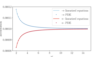
Both forces are always positive (or zero), regardless of the direction of the incoming wave. This means that if the wave is coming from the left, we observe the positive radiation pressure (PRP) and when it is coming from the right, we see the negative radiation pressure (NRP). For :
| (28) |
which is not surprising, since then also and the waves on both sides become more similar to each other. For waves with different directions behave differently:
| (29) |
5 Numerical results
To check the validity of the approximate effective forces (27), the equations (4) were solved numerically, and the results were compared. The initial condition was the domain wall and the ‘wave train’
| (30) |
for the wave going from left to right or
| (31) |
for the wave propagating from right to left, where , are group velocities and with . The RK4 method was used, with space and time steps and respectively. Accelerations were measured by fitting the quadratic function to the position of the soliton in the time range to .
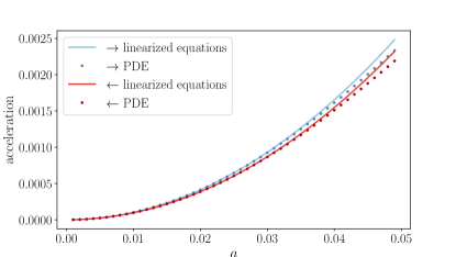
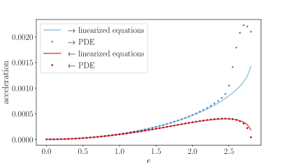
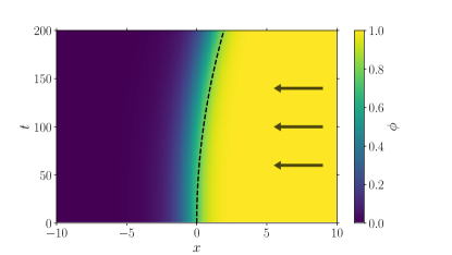
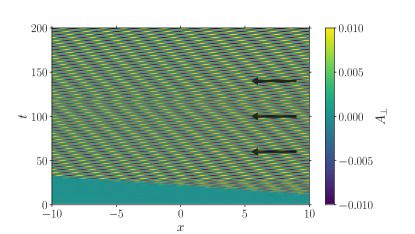
The results, presented in figures 1, 2 and 3, agree well with the approximate formulas derived from the linearized equations. An example of the soliton evolution with NRP can be seen in the figure 4. As expected, the accuracy of the approximation drops for larger amplitudes (Fig. 2), and charges (Fig. 3), due to the nonlinear effects.
6 Conclusions
Using the linearized Newtonian approximation and numerical simulations, we have shown that the domain walls always accelerate towards vacuum. Therefore, we observe both PRP and NRP, depending on the direction of the incoming wave. This behavior is very similar to the one observed in the model without a gauge field [24], and we expect that it would play a similar role in multikink collisions, although it requires further study.
Another possibility for further research would be to study oscillons and their interactions with kinks. Oscillons can play an important role in many physical processes and have interesting, nontrivial dynamics, and moreover, they can store enough energy to bounce back kinks [30]. Furthermore, radiation pressure exerted on more complicated topological solitons, i.e. vortices, can be studied in this model.
Observation of negative radiation pressure in (1+1) abelian Higgs model with a sextic potential is yet another indication that this phenomenon is widespread in theoretical physics. Although the results of this paper are not applicable to experiments directly, the studied system can be understood as an important simple toy model, expanding the mathematical tools needed to find NRP in nature.
Acknowledgements
This work has been supported by the Priority Research Area under the program Excellence Initiative – Research University at the Jagiellonian University in Kraków. The author would also like to express the gratitude to Tomasz Romańczukiewicz for useful discussions.
References
- [1] A R Bishop. Solitons in condensed matter physics. Physica Scripta, 20(3-4):409, sep 1979.
- [2] Nicholas S Manton. Skyrmions: A theory of nuclei. World Scientific, 2022.
- [3] D J Frantzeskakis. Dark solitons in atomic Bose–Einstein condensates: from theory to experiments. Journal of Physics A: Mathematical and Theoretical, 43(21):213001, may 2010.
- [4] Boris A Malomed. Variational methods in nonlinear fiber optics and related fields. Progress in optics, 43(71), 2002.
- [5] T W B Kibble. Topology of cosmic domains and strings. Journal of Physics A: Mathematical and General, 9(8):1387, aug 1976.
- [6] Péter Forgács and Árpád Lukács. Stabilization of semilocal strings by dark scalar condensates. Phys. Rev. D, 95:035003, Feb 2017.
- [7] Tanmay Vachaspati. Kinks and Domain Walls: An Introduction to Classical and Quantum Solitons. Cambridge University Press, 2006.
- [8] Nicholas Manton and Paul Sutcliffe. Topological Solitons. Cambridge Monographs on Mathematical Physics. Cambridge University Press, 2004.
- [9] David K. Campbell, Michel Peyrard, and Pasquale Sodano. Kink-antikink interactions in the double sine-Gordon equation. Physica D: Nonlinear Phenomena, 19(2):165–205, 1986.
- [10] N. H. Christ and T. D. Lee. Quantum expansion of soliton solutions. Phys. Rev. D, 12:1606–1627, Sep 1975.
- [11] Tadao Sugiyama. Kink-Antikink Collisions in the Two-Dimensional Model. Progress of Theoretical Physics, 61(5):1550–1563, 05 1979.
- [12] David K. Campbell, Jonathan F. Schonfeld, and Charles A. Wingate. Resonance structure in kink-antikink interactions in theory. Physica D: Nonlinear Phenomena, 9(1):1–32, 1983.
- [13] Roy H. Goodman and Richard Haberman. Kink-antikink collisions in the equation: The n-bounce resonance and the separatrix map. SIAM Journal on Applied Dynamical Systems, 4(4):1195–1228, 2005.
- [14] A. Alonso Izquierdo, J. Queiroga-Nunes, and L. M. Nieto. Scattering between wobbling kinks. Phys. Rev. D, 103:045003, Feb 2021.
- [15] N. S. Manton, K. Oleś, T. Romańczukiewicz, and A. Wereszczyński. Collective coordinate model of kink-antikink collisions in theory. Phys. Rev. Lett., 127:071601, Aug 2021.
- [16] C. Adam, N. S. Manton, K. Oles, T. Romanczukiewicz, and A. Wereszczynski. Relativistic moduli space for kink collisions. Phys. Rev. D, 105:065012, Mar 2022.
- [17] C. Adam, D. Ciurla, K. Oles, T. Romanczukiewicz, and A. Wereszczynski. Relativistic moduli space and critical velocity in kink collisions. Phys. Rev. E, 108:024221, Aug 2023.
- [18] G.C. Katsimiga, F.K. Diakonos, and X.N. Maintas. Classical dynamics of the Abelian Higgs model from the critical point and beyond. Physics Letters B, 748:117–124, 2015.
- [19] S. Raby and A. Ukawa. Instantons in (1 + 1)-dimensional abelian gauge theories. Phys. Rev. D, 18:1154–1173, Aug 1978.
- [20] P. Forgács and Z. Horváth. Topology and saddle points in field theories. Physics Letters B, 138(5):397–401, 1984.
- [21] Glennys R. Farrar and John W. McIntosh. Scattering from a domain wall in a spontaneously broken gauge theory. Phys. Rev. D, 51:5889–5904, May 1995.
- [22] Tomasz Romańczukiewicz. Interaction between kink and radiation in model. Acta Phys. Polon. B, 35:523–540, 2004.
- [23] Peter Forgács, Árpád Lukács, and Tomasz Romańczukiewicz. Negative radiation pressure exerted on kinks. Phys. Rev. D, 77:125012, 2008.
- [24] Tomasz Romańczukiewicz. Could the primordial radiation be responsible for vanishing of topological defects? Physics Letters B, 773:295–299, 2017.
- [25] Patrick Dorey, Kieran Mersh, Tomasz Romańczukiewicz, and Yasha Shnir. Kink-antikink collisions in the model. Phys. Rev. Lett., 107:091602, Aug 2011.
- [26] Péter Forgács, Árpád Lukács, and Tomasz Romańczukiewicz. Plane waves as tractor beams. Phys. Rev. D, 88:125007, Dec 2013.
- [27] Dominik Ciurla, Péter Forgács, Árpád Lukács, and Tomasz Romańczukiewicz. Negative radiation pressure in Bose-Einstein condensates. Phys. Rev. E, 109:014228, Jan 2024.
- [28] Tomasz Romańczukiewicz. Negative radiation pressure in case of two interacting fields. Acta Phys. Polon. B, 39:3449–3462, 2008.
- [29] R.D. Yamaletdinov, T. Romańczukiewicz, and Y.V. Pershin. Manipulating graphene kinks through positive and negative radiation pressure effects. Carbon, 141:253–257, 2019.
- [30] Patrick Dorey, Anastasia Gorina, Tomasz Romańczukiewicz, and Yakov Shnir. Collisions of weakly-bound kinks in the christ-lee model. Journal of High Energy Physics, 2023(9), September 2023.