compat=1.0.0
Identifying the transverse and longitudinal modes of the and mesons through their angular dependent decay modes
Abstract
Observing the mass shifts of chiral partners will provide invaluable insight into the role of chiral symmetry breaking in the generation of hadron masses. Because both the and mesons have vacuum widths smaller than 100 MeV, they are ideal candidates for realizing mass shift measurements. On the other hand, the different momentum dependence of the longitudinal and transverse modes smear the peak positions. In this work, we analyze the angular dependence of the two-body decays of both the and . It is found that the longitudinal and transverse modes of the can be isolated by observing the pseudoscalar decay in either the forward or perpendicular directions, respectively. For the decaying into a vector meson and a pseudoscalar meson, one can accomplish the same goal by further observing the polarization of the vector meson through its angular dependence on the two pseudoscalar meson decay.
I Introduction
Understanding the generation of hadron masses stands as one of the fundamental puzzles in Quantum Chromodynamics (QCD). It is widely believed that spontaneous chiral symmetry breaking Nambu:1961tp ; Nambu:1961fr partly contributes to the generation of hadronic masses Hatsuda:1985eb ; Brown:1991kk ; Hatsuda:1991ez ; Leupold:2009kz . Experiments conducted worldwide have aimed to observe the mass shift of hadrons at finite temperatures or densities Hayano:2008vn ; JPARC:2023quf ; Metag:2017yuh ; Ohnishi:2019cif ; Salabura:2020tou . This is because chiral symmetry is expected to be partially restored in the initial stages of relativistic heavy ion collisions and in nuclear matter probed by nuclear target experiments, respectively.
In particular, the J-PARC E16 experiment JPARC:2023quf ; Aoki:2023qgl will pursue the observation of the mass shift of the meson through pairs emanating from pA collisions. This measurement will be complemented by the J-PARC E88 experiment Sako , which aims to measure the meson through its decay. The is expected to be a particularly sensitive probe, as its vacuum width is small, meaning that any width increase in the medium will not be significant enough to disrupt experimental reconstruction of the peak position Gubler:2024day .
On the other hand, to isolate the effect of chiral symmetry restoration in a medium, the transformation of chiral partners towards degeneracy would be a critical experimental signal. This inevitably leads us to study the system as they appear to be the only realistically observable chiral partners, of which both have small vacuum widths Lee:2019tvt ; Song:2018plu .
The existence of the spin degrees of freedom, however, makes the situation more complicated, as both vector and axial vector mesons will have different responses depending on their spin orientation with respect to their motion relative to the medium. This effect is dominated by non-chiral symmetry-breaking effects Lee:2023ofg , but it will cause the longitudinal and transverse modes to diverge for larger momenta, obscuring the peak position Lee:1997zta ; Kim:2019ybi .
In a recent publication Park:2022ayr , we have shown that the longitudinal and transverse modes of the meson can be discriminated by analyzing the angular dependence of its two-body decay. In particular, the and decays can be used as complementary measurements.
In this work, we analyze the angular dependence of the two-body decays of both the and . As we will show, the longitudinal and transverse modes of the , or any other vector meson such as the (which decays from ) can be isolated by observing the pseudoscalar decay in either the forward or perpendicular directions, respectively. For the decaying into a vector meson and a pseudoscalar meson, one can accomplish the same goal by further observing the polarization of the vector meson as discussed before.
The paper is organized as follows. In Sec.II, we introduce the relevant effective interaction Lagrangians and estimate the coupling constants for each decay. Then we study a spin-1 particle state with a superposition of three different helicities and discuss how the general angular distribution is connected to the spin density matrix. We furthermore point out that the same result can be obtained using the helicity formalism. We then summarize our discussion in Section.III. More details regarding the calculations are provided in the appendices.
II (Axial)Vector meson decay rate
In this section, we will introduce the basic kinematics of the two-body decay channels, along with phenomenological Lagrangians describing the interactions between the relevant particles, and estimate the corresponding hadronic coupling constants. We closely analyze the decay channels and , both of which will be denoted as . For the decays, we study and . Here denotes a pseudoscalar meson while and denote a vector meson and an axial vector meson, respectively. In the decay, we will denote and as polar and azimuthal angles of one of the decay products, measured in the center of mass (c.m.) frame (see Fig. 1). The z-axis is defined to align with the momentum direction of the initial particle in the Lab frame.
We assume that the initial (axial)vector meson is a superposition of the different helicity states (: transverse polarization, : longitudinal polarization) with respective amplitudes . We can hence express the general (axial)vector meson state as
| (1) |
The spin density matrix is defined using the coefficients and reads
| (2) |
The trace of the spin density matrix is normalized to 1: . For a transversely polarized (axial)vector meson, the meson spin component will be , thus . In contrast, if the meson is longitudinally polarized, and . The density matrix of an unpolarized meson has diagonal entries of 1/3, specifically .
II.1 and decay
The phenomenological interaction Lagrangians of the vector meson with two pseudoscalar mesons used in this work, are adapted from Ref.Sung:2021myr and given as
| (3) | |||
| (4) |
are isomultiplets, their matrix representation being listed in Appendix A. All the masses of isomultiplets are isospin averaged using the PDG data Workman:2022ynf , giving MeV, MeV, MeV and MeV. Similarly, in order to evaluate the coupling constants and , we use the partial decay width from the PDG Workman:2022ynf . The initial spin average involves a total of 3 degrees of freedom. For , depending on the isospin, the decay modes are and . For the decay, they are and . Therefore, after summing over the initial isospin components, the average is obtained by dividing by a factor of 3 for and 4 for . The respective widths are then obtained as
where
is the momentum of the two produced particles in the c.m. frame, while stands for the mass of the initial particle. For the decay, is taken to be one of the outgoing mesons. For the decay, is the mass of the produced vector-meson. From the partial decay width of the initial vector-meson, we can obtain the coupling strength of each decay channel. The resultant coupling constants of the respective interaction Lagrangians are listed in Table 1.
Assuming that the initial vector-meson is in the general configuration of Eq. (1), we can obtain the general angular distribution as Schilling:1969um
| (6) |
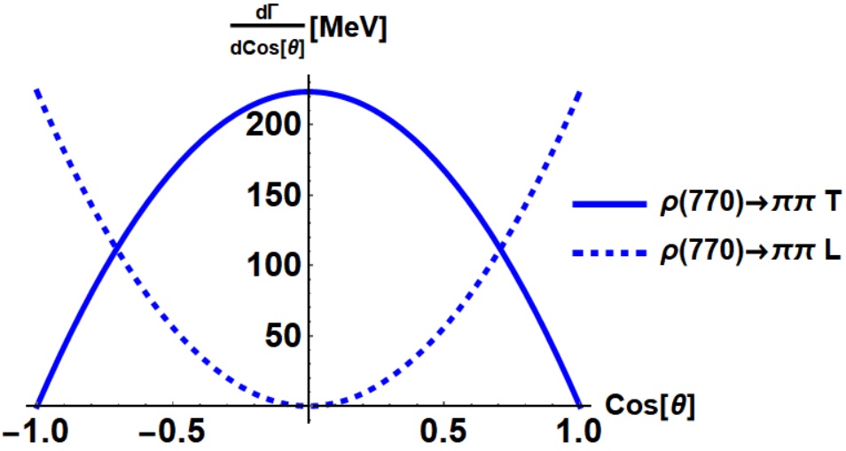
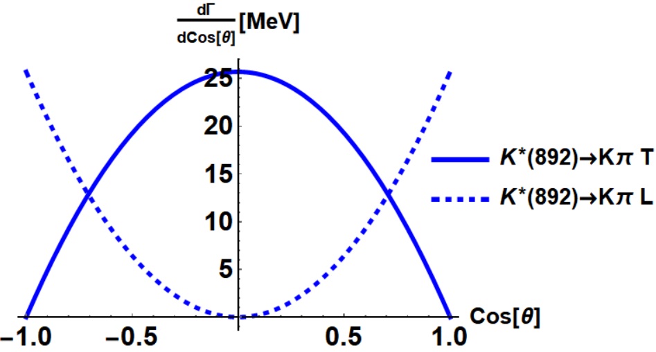
where and are as before the polar and azimuthal angles of the outgoing daughter particle. The details of this calculation are given in the Appendix B. Integrating over , we acquire the polar distribution as
| (7) |
If we substitute , becomes the decay distribution of a transversely polarized vector meson, while for , we get its longitudinal counterpart. These results agree with the result derived using polarization tensor Park:2022ayr .
| Decay | ||||
|---|---|---|---|---|
| (MeV) | ||||
II.2 and decay
The Lagrangian characterizing the coupling between the axial vector meson and a vector and pseudoscalar meson Sung:2021myr is given as
| (8) |
The matrix representation of the field is given in Appendix A.
As before, we first compute the partial decay widths using the above interactions, giving
The partial decay widths of the decay channels are taken from the PDG Workman:2022ynf . Following the same procedure as in the previous subsection, the angular dependence of the decay distribution is obtained as
| (10) | |||
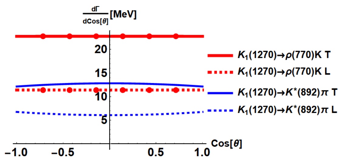
Integrating over , we again get the polar angle distribution
| (11) | |||
The angular dependence of this distribution is shown in Fig. 3. Unfortunately, unlike the case shown in Fig. 2, one can not isolate the different initial polarization by looking at different decay angles, which can be understood from the suppression factor ( () appearing in the second term in the large bracket of Eq. (11).
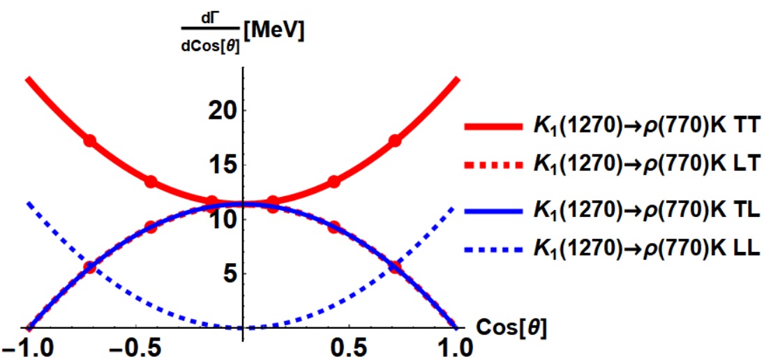
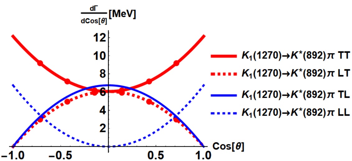
To overcome this, it is however possible to measure the polarization of the final vector-meson by again using the angular distribution as shown in Fig. 2. Then, there are a total of four possible combinations of initial and final vector-meson polarizations. Each decay amplitude is listed below.
| (12) | ||||
The first and second subscripts of ( or ) here represent the polarization of an initial and final vector-meson, respectively. The corresponding results are shown in Fig. 4. As can be seen there, once we measure the transverse component of the final vector meson for both decay modes, one can isolate the transverse component by looking at the forward or backward direction. Conversely, when we measure the longitudinal component of the final vector meson, one can isolate the longitudinal component by again looking at the forward or backward direction. The improvement compared to the situation shown in Fig. 3 is clear.
II.3 Helicity basis and Wigner -matrix
So far, we have computed the general angular decay distribution by using the respective interaction Lagrangian for each decay channel. Here, we shall see that the same angular distribution is reproduced by taking advantage of the helicity formalism. As the basic ingredient, we need the Wigner -matrix and the density matrix of an initial (axial)vector-meson. The convention for the Wigner -matrix is adopted from that of Ref. Chung:1971ri and devanathan2005angular . The helicity basis for a massive particle is labeled by its momentum and helicity and is obtained by a boost along -direction from the rest state followed by the rotation described by an Euler angle .
| (13) |
By applying a Wigner -matrix, we rotate the density matrix so that the quantization axis rotates from the -axis to align with the direction of momentum of an outgoing particle, specified by the angles and .
| (14) |
Here, , where and are the helicities of the daughter particles of mass and , respectively. here stands for the interaction Hamiltonian for each helicity component of corresponding decay, which we can calculate from the interaction Lagrangians given before. More details regarding this calculation are explained in Appendix C.
III Summary and Conclusions
In this work, we have shown that one can isolate the initial longitudinal and transverse modes of the and from observing the decay angles and polarizations of their decay particles. In particular, for , this is possible by measuring the decay angle distributions of the outgoing pseudoscalar mesons. For , one furthermore needs to determine the polarization of the outgoing vector meson to disentangle the longitudinal and transverse modes.
Such a measurement should be feasible in a future J-PARC experiment. This will help to reduce the uncertainty of the mass shift measurement of these two particles in nuclear matter. Once this is realized, the chiral partner nature of and may be experimentally confirmed, which will bring us one step closer to understanding the role of chiral symmetry breaking and restoration to the generation of hadron masses.
Acknowledgments
This work was supported by the Samsung Science and Technology Foundation under Project No. SSTF-BA1901-04, and by the Korea National Research Foundation under grant No. 2023R1A2C3003023 and No. 2023K2A9A1A0609492411, JSPS KAKENHI Grants No. JP19KK0077, No. JP20K03940, No. JP21H00128, No. JP21H00128, and No. JP21H01102, for the Promotion of Science (JSPS). The work was also supported by the REIMEI project of JAEA under the title “Studying the origin of hadron masses through the behavior of vector mesons in nuclear matter from theory and experiment”.
Appendix A Effective interaction Lagrangian
, and isodoublet matrices are defined as
| (15) |
Direct matrix multiplication yields the interaction Lagrangian as
| (16) | ||||
| (17) | ||||
| (18) | ||||
Appendix B Disentangling the polarizations of a vector-meson using the polarization tensor and vector
We will in this appendix discuss two methods to disentangle the contributions of different polarization components of vector mesons to their decay amplitudes. The first one makes use of the polarization tensor and can only be used for purely transversely or longitudinally polarized vector/axial-vector mesons. The second more general method uses the polarization vector and can be applied to an arbitrary spin configuration. For the first method, we first need to define the polarization tensors as
| (19) |
Contracting these polarization tensors with the decay amplitude, we can disentangle its transverse and longitudinal parts. and here stand for the energy and momentum of the considered vector/axial-vector meson. In what follows, we will display the decay as an example of and the decay as an example of . The same method can also be applied to and , respectively. The decay amplitudes for the two cases are obtained as
| (20) | ||||
Contracting these with the above polarization tensors, taking the final spin sum (if applicable), we get
| (21) |
and
| (22) |
The different factors 2 and 1 appearing in the fist terms within the large brackets in Eq. (22) are due to the different degeneracy factors of the two transverse and one longitudinal modes for a massive spin-1 particle.
Let us next move on to the second method, in which we can further study the contributions of the different helicity states and their mixing. The polarization vectors of the initial particle in its own rest frame for each helicity state are given as
| (23) |
where is the general polarization vector (that will be more explicitly discussed further below) with being the particle momentum and its helicity. Taking the absolute square of the invariant amplitude
| (24) |
yields the general angular distribution which can be expressed as
| (25) |
where is defined in Eq. (2).
For the decay, we also need the polarization vector of the produced vector-meson in the rest frame of the initial axial vector-meson, which is obtained by an inverse Lorentz boost along -axis followed by an Euler rotation . here rotates the object about the -axis by an angle of , followed by a rotation around the -axis by an angle of , and finally followed by an angle of around the -axis. The polarization vectors of the produced vector-meson in the c.m. frame are then obtained as
| (26) |
here is the energy of the produced vector-meson in the c.m. frame. The general angular distribution is calculated as
| (27) | ||||
| (28) | ||||
Appendix C More details about the helicity formalism
The two-body decay process is considered starting from a definite angular momentum state of in the mother particle rest frame, decaying into two particle helicity state , where and are the relative momenta and helicity difference, respectively, between the two decaying particles denoted with subscripts 1 and 2. The notation and derivation of this section are adapted from Ref. Chung:1971ri .
C-1 One particle state
First, we study the single-particle canonical and helicity states. The canonical state is defined as a state labeled by its momentum, total angular momentum and its -component. A general canonical state with arbitrary momentum pointing in the , direction is then constructed by first inversely rotating the particle such that it aligns with the z-axis, followed by a Lorentz boost in the z-direction, and finally a rotation back into the momentum direction of the particle with polar angles ,
| (29) |
where is a Lorentz boost along the -axis. When the particle is at rest, the canonical state transforms under rotation as
| (30) |
where is a linear representation of a rotation operator Chung:1971ri .
The helicity state is labeled by the momentum, total angular momentum and helicity. It is similarly constructed by firstly Lorentz boosting the rest state (which is here defined such that is the eigenstate of the z-component of the angular momentum, it is thus the same as with ). along the z-axis followed by a rotation such that the momentum points into the direction specified by the polar angles and . We thus have
| (31) |
The relation between canonical and helicity states is given as
| (32) |
We here choose our normalization to be Lorentz invariant, such that
| (33) |
C-2 Two particle state
By definition, the two particle helicity state is a tensor product of two one particle states in the c.m. frame,
| (34) |
We next derive the relation between the two particle helicity state and a state of definite angular momentum . Here, and denote the total angular momentum and its projection onto the -axis of the initial particle, respectively. We assume that the above general two particle helicity state, with the momentum of one particle specified by the angles in the c.m. frame, is related to the total angular momentum state by a coefficient as
| (35) |
Let us here derive an explicit expression for . The standard helicity state is defined for the state where ,
| (36) |
In the standard state, particle 2 is heading towards the negative -direction, thus its projection on the -axis is . Therefore, total angular momentum projection . By a definition of two particle helicity state, it can also be viewed as a state which is rotated from the standard state. Hence,
| (37) |
where we have in the last line made use of the fact that a state of definite angular momentum behaves the same way as given in Eq. (30). Making use of proper orthogonality relations of the states and and properties of the rotation matrix (see for example Ref. Chung:1971ri for more details), we obtain as
| (38) |
and, comparing Eq. (35) with the last line of Eq. (37), we finally have
| (39) |
where again .
C-3 Two body decay amplitude
The two body decay amplitude is a transition amplitude from a definite angular momentum state of the initial particle to a two particle helicity state of the daughter particles in the c.m. frame. The transition amplitude from to is given as below,
| (40) |
where Eq. (39) and angular momentum conservation was used in the second line. here stands for the interaction Hamiltonian describing the decay. Making use of the fact that this is a scalar quantity, the matrix element cannot depend on , but only on the rotational invariants , and . We will hence denote it as in what follows.
If we specify the initial state as superposition of the different quantum numbers, specifically and in analogy to Eq. (2) define the spin density matrix as , the normalized angular distribution of this decay can be given as , where is the decay width of the initial particle. We hence obtain
| (41) |
For the decay, only the matrix element is needed, and the angular decay distribution is therefore automatically fixed only from the rotation matrix , given in Eq. (13). As a result, we obtain
| (42) | ||||
which agrees with Eq. (6).
On the other hand, for the decay, the three matrix elements , and need to be considered. Confining us here to strong and thus parity conserving decay, we can make use of the symmetry property of and are hence left with two independent terms, which have to be determined from a specific interaction Hamiltonian. In this work, it can be easily obtained from the interaction Lagrangian given in Eq. (8) and . Next, we compute the transition amplitude of Eq. (40) using the polarization vectors given in Appendix B. To determine the relative strength of the two terms, we only need two independent transition amplitudes, with with an outgoing vector particle carrying a different helicity . Specifically, we have
| (43) |
and
| (44) |
Comparing this with Eq. (40), we note that
| (45) |
and
| (46) |
This is sufficient to derive the angular distribution of the decay as
| (47) | ||||
which agrees with Eq. (10).
References
- (1) Y. Nambu and G. Jona-Lasinio, Phys. Rev. 122, 345-358 (1961).
- (2) Y. Nambu and G. Jona-Lasinio, Phys. Rev. 124, 246-254 (1961).
- (3) T. Hatsuda and T. Kunihiro, Phys. Rev. Lett. 55, 158 (1985).
- (4) G. E. Brown and M. Rho, Phys. Rev. Lett. 66, 2720 (1991).
- (5) T. Hatsuda and S. H. Lee, Phys. Rev. C 46, no. 1, R34 (1992).
- (6) S. Leupold, V. Metag and U. Mosel, Int. J. Mod. Phys. E 19, 147 (2010).
- (7) For review see, R. S. Hayano and T. Hatsuda, Rev. Mod. Phys. 82, 2949 (2010).
- (8) M. Ichikawa et al., “Commissioning Runs of J-PARC E16 Experiment,” Acta Phys. Polon. Supp. 16, no.1, 143 (2023).
- (9) V. Metag, M. Nanova and E. Y. Paryev, Prog. Part. Nucl. Phys. 97, 199 (2017).
- (10) H. Ohnishi, F. Sakuma and T. Takahashi, Prog. Part. Nucl. Phys. 113, 103773 (2020).
- (11) P. Salabura and J. Stroth, [arXiv:2005.14589 [nucl-ex]].
- (12) K. Aoki et. al, Few Body Syst. 64, 63 (2023).
- (13) H. Sako et. al, ”P88: Study of in-medium modification of mesons inside the nucleus with measurement with the E16 spectrometer”, https://j-parc.jp/researcher/Hadron/en/pac_2107/pdf/P88_2021-12.pdf
- (14) P. Gubler, E. Bratkovskaya, M. Ichikawa and T. Song, EPJ Web Conf. 291, 04003 (2024).
- (15) S. H. Lee, JPS Conf. Proc. 26, 011012 (2019) [arXiv:1904.09064 [nucl-th]].
- (16) T. Song, T. Hatsuda and S. H. Lee, Phys. Lett. B 792, 160-169 (2019) [arXiv:1808.05372 [nucl-th]].
- (17) S. H. Lee, Symmetry 15, no.4, 799 (2023) [arXiv:2303.14415 [hep-ph]].
- (18) S. H. Lee, Phys. Rev. C 57, 927-930 (1998) [erratum: Phys. Rev. C 58, 3771 (1998)] [arXiv:nucl-th/9705048 [nucl-th]].
- (19) H. Kim and P. Gubler, Phys. Lett. B 805, 135412 (2020) [arXiv:1911.08737 [hep-ph]].
- (20) I. W. Park, H. Sako, K. Aoki, P. Gubler and S. H. Lee, Phys. Rev. D 107, no.7, 074033 (2023) [arXiv:2211.16949 [hep-ph]].
- (21) H. S. Sung, S. Cho, J. Hong, S. H. Lee, S. Lim and T. Song, Phys. Lett. B 819, 136388 (2021) [arXiv:2102.11665 [nucl-th]].
- (22) R. L. Workman et al. [Particle Data Group], PTEP 2022, 083C01 (2022).
- (23) K. Schilling, P. Seyboth and G. E. Wolf, Nucl. Phys. B 15, 397-412 (1970) [erratum: Nucl. Phys. B 18, 332 (1970)].
- (24) S. U. Chung, doi:10.5170/CERN-1971-008.
- (25) V. Devanathan, Angular Momentum Techniques in Quantum Mechanics, (Springer Netherlands, 2005)