Frozen Gaussian approximation for the fractional Schrödinger equation
Lihui Chai111School of Mathematics, Sun Yat-sen University, Guangzhou, 510275, China (chailihui@mail.sysu.edu.cn).Hengzhun Chen222School of Mathematical Sciences, Fudan University, Shanghai, 200433, China(hengzhunchen21@m.fudan.edu.cn).Xu Yang333Department of Mathematics, University of California, Santa Barbara, CA 93106, USA (xuyang@math.ucsb.edu).
Abstract
We develop the frozen Gaussian approximation (FGA) for the fractional Schrödinger equation in the semi-classical regime, where the solution is highly oscillatory when the scaled Planck constant is small. This method approximates the solution to the Schrödinger equation by an integral representation based on asymptotic analysis and provides a highly efficient computational method for high-frequency wave function evolution. In particular, we revise the standard FGA formula to address the singularities arising in the higher-order derivatives of coefficients of the associated Hamiltonian flow that are second-order continuously differentiable or smooth in conventional FGA analysis. We then establish its convergence to the true solution. Additionally, we provide some numerical examples to verify the accuracy and convergence behavior of the frozen Gaussian approximation method.
1 Introduction
We consider the Schrödinger equation
(1.1)
where in the semi-classical regime, is the complex-valued wavefunction, and the Hamiltonian operator is defined by a pseudo-differential operator [10, 16] associated with a symbol ,
(1.2)
We assume simply the symbol of the Hamiltonian takes the form of
(1.3)
with and corresponding to the symbols of kinetic energy and potential energy, respectively.
For example, when , , one has the standard semi-classical Schrödinger equation, and in general when , , one has the fractional Schrödinger equation,
(1.4)
where, for , the fractional Laplacian is defined as the inverse Fourier transformation of the :
(1.5)
and in general, the kinetic operator
(1.6)
In the above equations, we have used the Fourier transformation and its inverse transformation denoted as follows:
(1.7)
(1.8)
The semiclassical Schrödinger equation (1.1) has been studied intensively in both theoretical and numerical aspects, see e.g., [37, 29, 10, 4] and [3, 8, 11, 34, 19]. Most of these methods require the Hamiltonian symbol to be a polynomial in or have a certain smoothness, even up to . However, for the fractional Schrödinger equation, when , the symbol is only in . Although one can apply similar methods formally, the convergence results are not yet clear.
The fractional Schrödinger equation was first introduced by Laskin in [24, 25, 26], where the path integral was generalized from Brownian-type quantum mechanics trajectory to Lévy-type quantum mechanics trajectory, to represent the Bohr atom, and fractional oscillator, and to study the quantum chromodynamics (QCD) problem of quarkonium.
The fractional Schrödinger equation with can also be used as a toy model in the mathematical description of the dynamics of semi-relativistic boson stars in the mean-field limit [9, 28].
The fractional Schrödinger equation has been investigated numerically using finite difference method [17] and time-splitting spectral method [7, 38].
The properties of nonlinear fractional Schrödinger equations such as global existence, the possibility of finite time blow-up, the existence and stability of the ground states, and decoherence of the solution are studied numerically using Fourier spectral methods in [23, 2, 22].
Numerical methods with perfectly matched layers (PMLs) in both real-space and Fourier-space for linear fractional Schrödinger equations have been proposed in [1].
In this paper, we derive a frozen Gaussian approximation (FGA) for the fractional Schrödinger equation and show the convergence in the semi-classical regime. The FGA was originally used in quantum chemistry [14, 15] with systematic justifications for the Schrödinger equation in [20, 21, 36, 27]. Then the FGA theory was generalized to linear strictly hyperbolic systems by the pioneer works [30, 31], and recently to non-strictly hyperbolic systems such as the elastic wave equations [13], relativistic Dirac equations in the semi-classical regime [6, 5], non-adiabatic dynamics in surface hopping problems [32, 33, 18].
The FGA propagates the wavefield through the classical ray center and complex-valued amplitude which are determined by the associated Hamiltonian flow. Given the coefficients of the equation smooth enough (at least in ), one can obtain the FGA equations along the ray path by asymptotic expansion concerning the semi-classical parameter and prove the convergence in the first-order of (higher-order can be obtained if performing further expansion). However, when some coefficient is not in , e.g. , the fractional Schrödinger equation with , the expansion may break down and one faces the problem of propagation of the ray path governed by the Hamiltonian system with singularities. In this situation, the convergence of the FGA is not guaranteed by the existing theory. To overcome this difficulty, we introduce a regularization parameter when deriving the FGA formulation, and by looking carefully into the residual terms in the expansion and tuning the parameter incorporate with we can bound the high-order derivatives of the Hamiltonian flow and obtain a convergence result. The other difficulty in dealing with the fractional Hamiltonian system is that if we do asymptotic expansion in the physical space for the fractional Laplacian as it was usually done for the existing FGAs (Lemma 2), there will be some nasty items which are not easy to estimate, so we propose the asymptotic expansion for the fractional Laplacian in the momentum space (Lemma 3) and obtain a compact form of the remainder terms which allow us to perform convergence analysis more easily.
The rest of this paper is organized as follows: In Section 2, we introduce the FGA for the fractional Schrödinger equation with preliminary results and a formal derivation, with the low-regularity issue of the Hamiltonian symbol not addressed. Then, in Section 3, we address the low-regularity issue in the formal derivation by employing a regularization technique and analyze the convergence of the FGA rigorously. The convergence result depends on the spatial dimensionality and the fractional order obtained. We present the numerical performance through numerical experiments in Section 4 and make conclusive remarks in Section 5.
Notations. The absolute value, Euclidean distance, vector norm, induced matrix norm, and the sum of components of a multi-index will all be denoted by . We use the notation and for the Schwartz class functions and smooth functions, respectively. We will sometimes use subscripts to specify the dependence of a constant on the parameters. Furthermore, it is worth noting that we utilize as the kinetic symbol and as the final time of evolution. The specific meanings of these symbols will be evident within the given context.
2 The frozen Gaussian approximation
In this section, we introduce the necessary concepts, assumptions, and preliminary results that will be utilized in deriving the frozen Gaussian approximation (FGA). While some of these have been systematically introduced in existing literature, such as [30, 31], we provide a concise overview for clarity. Subsequently, we present the initial formulation of the FGA for the fractional Schrödinger equation, and in Section 3, we will demonstrate its further modified version and convergence.
2.1 Hamiltonian flow and action
The Hamiltonian function corresponding to fractional Schrödinger equation (1.4) is defined as,
(2.1)
The Hamiltonian flow associated with solves
(2.2a)
(2.2b)
This gives the map
which is a canonical transformation defined as follows, with its proof similar to the counterpart presented in [31].
Definition 1(Canonical Transformation).
Let be a differentiable map,
We denote the Jacobian matrix as
(2.3)
We say that is a canonical transformation if is symplectic for any , i.e.
(2.4)
where is the -dimensional identity matrix.
To facilitate the analysis of the FGA, it is convenient to introduce the operator and the matrix associated with canonical transformation , defined as follows:
(2.5)
Furthermore, we present the following Lemma, the proof of which relies solely on the symplecticity of the Jacobian matrix associated with the canonical transformation . For detailed proof, please refer to [31].
Lemma 1.
is invertible for with .
Next, we give the definition of action associated with Hamiltonian flow .
Definition 2(Action).
Suppose is a canonical transformation, then a function is called an action associated with if it satisfies
(2.6)
(2.7)
The action corresponding to canonical transformation solves
(2.8)
with initial condition . It is easy to check that the solution of the equation above is indeed the action associated with , which is given by
2.2 Fourier integral operator
The frozen Gaussian approximation can be formulated using the Fourier integral operator, a commonly used definition in the relevant literature:
Definition 3(Fourier Integral Operator).
For Schwartz-class functions and , we define the Fourier Integral Operator with symbol as
(2.9)
where the complex-valued phase function is given by
(2.10)
In preparation for the subsequent derivation and convergence analysis, we say two functions are equivalent if they give the same Fourier integral, precisely we introduce the following definition:
Definition 4.
Given in Schwartz class, we say that and are equivalent, denoted as , if
(2.11)
for any function .
Furthermore, we refer to Lemma 5.2 in [31], which provides the equivalent asymptotic orders for the terms in the subsequent expansion we will introduce. This lemma plays a crucial role in deriving the standard frozen Gaussian approximation. To ensure clarity in notation, we state the lemma as follows, utilizing the Einstein summation convention for repeated indices:
Lemma 2.
For any -vector function and any matrix function in Schwartz class, we have
(2.12)
and
(2.13)
Suppose is a tensor in Schwartz class viewed as function of , then we have
(2.14)
or equivalently,
(2.15)
Here we use to denote the inverse matrix of . More precisely, , and the -th entry of is denoted as .
Unlike the conventional asymptotic order analysis in frozen Gaussian approximation, which relies on the phase function (2.10) and its equivalent asymptotic order Lemma 2, we go beyond that by introducing the concept of the dual phase function and its corresponding action function. This extension allows us to effectively handle the kinetic term in the fractional Schrödinger equation (1.4). The dual-phase function is defined as
(2.16)
and the dual action is defined as the unique solution of
(2.17)
We remark here that the difference between and is
(2.18)
Additionally, it is straightforward to verify that satisfies
(2.19)
and we have the following relation,
(2.20)
These relations are analogous to their counterparts in the original phase function and action, which lead to a parallel asymptotic order analysis presented in the lemma below for the Fourier integral operator with dual phase function defined as
where and are Schwartz-class functions.
Lemma 3.
For any -vector function and any matrix function in Schwartz class, we have
(2.21)
and
(2.22)
Suppose is a tensor in Schwartz class viewed as function of , then we have
Now we introduce the Fourier-Bros-Iagolnitzer (FBI) transform, which can be regarded as a component of the Fourier integral operator and be useful in our convergence analysis.
For , define the FBI transformation ( used for kinetic part and used for potential part) on as
(2.25)
(2.26)
For one can easily verify that given function and its Fourier transform ,
(2.27)
The pseudo inverse FBI transformation on is given by
(2.28)
(2.29)
We have the following property for the FBI transformation whose proof can be found in [35].
Proposition 1.
For any ,
(2.30)
Hence the domain of and can be extended to and , respectively. Moreover, but .
2.3 Formulation of the frozen Gaussian approximation
The (1st-order) frozen Gaussian approximation (FGA) is defined as
(2.31)
where is the initial condition, is defined in (2.10) with the position center and the momentum center satisfying the Hamiltonian flow (2.2), the action satisfying (2.8), and the amplitude satisfying
(2.32)
Remark 1.
The readers may have noticed that to have a well-defined FGA system (2.2), (2.8) and (2.32) it requires the Hamiltonian in at least , which is not valid for the fractional Schrödinger equation. Here we perform formal derivation and leave the rigorous modification to the next section.
To see how the FGA solution fits the Schrödinger equation, we substitute (2.31) into the Schrödinger equation (1.1) and compute each term.
For the time-derivative term,
(2.33)
For potential function , using Taylor expansion of around ,
The term is zero by (2.2) and (2.8). For , noticing the fact that
(2.45)
(2.46)
one obtains that
(2.47)
where the last equation is implied by the evolutionary equation (2.32) for the amplitude. Thus, only the terms remain in (2.44), and we have
(2.48)
3 Convergence analysis
We have shown that the governing equation (2.48) for the FGA solution is formally an perturbation to the Schrödinger equation (1.1) if is bounded.
The remainder comes from the Taylor expansion for the Hamiltonian symbol, and thus it can be indeed bounded in the case that the Hamiltonian is smooth enough, for example, if . However, what we are interested in here is the case that the Hamiltonian may have singularities, for example, if we take in the fractional Schrödinger equation with , then the high-order derivatives of to are singular at . Notice that in (2.43) contains two parts: and , the Fourier transform is unitary in norm, and we have assumed that the initial is in Schwartz class, thus the analysis of the two parts of will follow the same state of art.
Then let’s assume that and consider general which may produce singularity at first.
The term comes from Taylor expansion of the kinetic symbol and it takes the form of
(3.1)
where determined by the rd order derivatives of . The above expressions of indicate that the remainder involves at least the th-order and at most the th-order derivatives of the kinetic symbol . The singularities in the high-order derivatives make the boundedness of difficult. On the other hand, we should also make it clear how to evolve the ODEs (2.2) and (2.32) when the trajectory touches the singularity at . To overcome these difficulties, we introduce a singularity-removed kinetic symbol by simply replacing by and define
(3.2)
And we consider as the solution of the Schrödinger equation defined by the kinetic symbol , i.e. ,
(3.3)
with the same initial condition . It can be verified that when is sufficiently small, closely approximates the solution of the original Schrödinger equation, . The proof of this assertion will be presented later.
However, while the modification addresses the evolution of ODEs in FGA when encountering singularities at , there might be singular points of the Hamiltonian equation (2.2) that possess constant solution with . To handle this issue, we introduce a cutoff with parameter for the initial condition of the Hamiltonian system to remove these singular points and ensure that no such singular points arise throughout the evolution.
In the following, we present a series of lemmas and propositions related to the construction of the approximation chain,
These results will be combined to establish the convergence in the proof of our main theorem.
Firstly we consider the cutoff to remove those singular points of the Hamiltonian system with constant solution . For , we define open set including singular points of Hamiltonian equations (2.2) as
(3.4)
Then we define the closed bounded set excludes those singular points as
(3.5)
For the Hamiltonian system over closed set , we have the following Lemma.
Lemma 4.
Given , if , satisfy Hamiltonian equations (2.2), then we have
(3.6)
for , , where is a constant.
Proof.
Denote one of the singular points of (2.2) as , then , . Consider closed set . Noticing that trajectory starts from will be a constant solution and all trajectories will not intersect during propagation, there will always be a positive distance between closed set and singular point . Thus,
(3.7)
Since is a continuous function over compact set , it will reach a minimum over , which completes the proof.
∎
Remark 2.
Lemma 4 mainly describes the phenomena that for a conserved system, if initial states are away from the equilibrium position (singular points of Hamiltonian equations) where momentum and force are zero at the same time, then the trajectory will not be stuck in a fixed point during propagation.
Let be a smooth cutoff function with so that
(3.8)
then for any , there exists constant such that
(3.9)
In parallel, we define the asymptotically high-frequency function. This definition is motivated by the WKB function, which is typical in the study of high-frequency wave propagation.
Let be a family of functions such that is uniformly bounded. Given , we say that is asymptotically high-frequency with cutoff if
(3.10)
and
(3.11)
as . is defined in (3.5) and notation means that for ,
if one denotes .
Remark 3.
Although in the definition above we use two constraints for and respectively, actually they are equivalent by (2.27) and only one of them need to be checked when verifying whether a function is asymptotically high-frequency or not.
Remark 4.
Closed bounded set defined in (3.5) over phase-space figures out where the initial wave function is “mainly” supported under the FBI transform and excludes the singular points of Hamiltonian equations (2.2) by small open ball regions, that is why we introduce the cutoff FGA.
Now we can define the frozen Gaussian approximation with cutoff as
(3.12)
To simplify notations, define a filtered version of amplitude as follows
(3.13)
then satisfies equation
(3.14)
From the definition of filtered amplitude, we know that the value of outside will not affect .
Since and satisfy the same equation with different initial data, the original FGA and cutoff FGA also satisfy the same differential equation (2.48) except that they have difference initial value, i.e. when ,
(3.15)
while
(3.16)
does not equal to .
We remark that, despite the slight difference in their initial values, it will not affect the convergence of FGA if we consider asymptotically high-frequency functions as initial conditions. A detailed discussion will be presented later in the proof of our main theorem.
Now we move forward to discuss the estimations of the Hamiltonian flow with the modified kinetic symbol . We make the following assumptions for the system (2.2) we considered, which will be assumed for the rest of the paper without further indication.
Assumption 1.
For smooth potential , there exists a constant such that
Despite the presence of singularities in the higher-order derivatives of at , the solution of the Hamiltonian flow (2.2) remains well-defined and unique. We conclude this property as the proposition stated below.
Proposition 2.
Consider the Hamiltonian function in (2.1)
with and smooth potential , then Hamiltonian equations (2.2)
have exact one solution under initial conditions .
Proof.
The proof of this proposition involves certain technical methods that are not directly relevant to the FGA itself, and therefore, we have included it in the Appendix A for reference.
∎
Corollary 1.
Perturbed momentum center and position center satisfy Hamiltonian flow (2.2) with modified kinetic symbol are continuous with respect to parameter .
Proof.
The proof can be done in the same way as Proposition 2.
∎
Now we can define the FGA solution for the modified Schrödinger equation (3.3), and follows the same arguments to derive (2.48) in Sec. 2.3 we obtain
(3.17)
Additionally, the cutoff strategy can be applied to the modified FGA solutions while maintaining the same properties.
Proposition 3.
For dynamic system with small enough, given we have
(3.18)
for , , where is a constant independent of .
Proof.
By the continuity of with respect to and it implies with .
∎
The introduction of the singularity-removed kinetic symbol leads to some new estimations relative to for most quantities appeared above.
We remark here that since the only difference between the FGAs for (3.3) and (1.1) is the kinetic symbol, the resulted remainders and are exactly in the same form, except changing to . So without causing misunderstandings, we will not introduce new notations but also use , , , and for the amplitude, action, position center, and momentum center and refer to the same equations in Section 2 to construct .
To complete the convergence analysis, we derive some properties for the solutions of the Hamiltonian flow and quantities in FGA ODEs, where the superscript is omitted for notation simplicity. Firstly we give two propositions to estimate and . Then we provide the order analysis concerning for their higher order derivatives in a compact form leveraging the associated canonical transformation. With these results, we can further analyze the order of the matrix, amplitude , and their higher order derivatives.
Proposition 4.
For the Hamiltonian flow (2.2) with the modified kinetic symbol , given initial conditions and an evolution time interval , when passes through its zero point at , there exists a small time interval, denoted as , whose length depends only on and , such that for , we have
(3.19)
where is a constant. Therefore, there are only a finite number of zero points of within a given finite evolution time interval.
Proof.
The proof of this proposition is based on the proof of Proposition 2 with some technical details and as such we put it in the Appendix B.
∎
Proposition 5.
Given , then for any and , we have
(3.20)
Furthermore,
where are constants.
Proof.
Differentiating with respect to time variable , from (2.2b) we have
where is a constant independent of . We will now divide the propagation of into two scenarios based on whether it has crossed the zero point. By utilizing Proposition 4 and Proposition 5, we can give an estimation of its boundedness. Without loss of generality, we may consider the evolution of starting from .
1.
. Denote , according to (3.20) we have for . Without loss of generality, we might set for notation simplicity. Given a such that within , we have
where for the last inequality we use and for . Thus,
Integrating both sides and noticing that
one has
for , where is independent of . After a certain period of propagation, may reach the value of zero and enter the second case.
2.
. By Proposition 4 it implies that there exist a small time interval , such that
where constant independent of time variable . Therefore, one has
In the same manner as the scenario when , we have
for , where is independent of . After propagation through a small time interval, one gets which comes back to the first case.
We remark that according to Proposition 4, there exists a finite number of zero points for within a given evolution time interval . Hence, combining the two scenarios above we prove the result for .
Next, we employ an induction argument to complete the proof.
Differentiating (3.23) with we have
(3.25)
Denote , , then we have
Hence, by Gronwall’s inequality, it implies
(3.26)
When , , note that , then we have
(3.27)
Similar to the case when , we always consider the bound for the integral like
in the two scenarios of during the propagation, i.e. , or .
Further, considering that either or is equal to and the other is equal to when , we can infer that . Therefore, we can derive that
which gives the result for since number of zero points of is finite within .
For general cases, suppose , denote , by induction we have
and
(3.28)
for and .
Besides, a similar estimate for the integral like
will be used in two scenarios of the evolution of .
Substituting these estimations into (3.26) produces
The matrix is invertible for and . Moreover, given , for ,
(3.30)
where are positive constants independent of .
Proof.
The invertiblity of and follows the same proof in [31, Lemma 5.1], which relies solely on the symplecticity of the associated Jacobian matrix . We will prove only the boundedness inequalities. For , note that
where is the adjugate matrix of , by Corollary 2 we have for .
For general cases, note that , given multi-indices such that , one has
By Corollary 2 and , comparing the order of at both sides of the equation above, we have , which completes the proof.
∎
Proposition 8.
For any and ,
Moreover, there exists positive constant and such that
(3.31)
Proof.
Firstly we prove the result for . Note that , from Proposition 6 one has
Additionally, by Proposition 7 one has . Thus, by (3.14) it implies
Using the same manner as Proposition 6 we have for .
For general cases when , note that the leading term of comes from the higher-order derivatives of with respect to , we have
with multi-indices .
Similar to the argument presented in Proposition 6, considering the order estimate provided by Proposition 7 for , we can arrive at our desired conclusion.
∎
Now we have gathered all the estimations of FGA quantities for convergence analysis.
Note that
we will discuss only the kinetic part in the following, the treatment of the potential part can be carried out in the same way, which is easier due to the smoothness of the potential function.
Let’s consider the remainder term caused by Taylor’s expansion of around , which takes the form of
(3.32)
where . On the right-hand side of the above equation, after expanding the partial derivative, each term is a product of a higher-order derivative of and higher-order derivatives of other FGA terms . We introduce the notation to denote these terms, where is the -th order derivative of , is a combination of higher-order derivatives of such that for with a constant factor . Here we abuse the notation to represent the original cutoff function supported in , as well as its higher-order partial derivatives with respect to . Additionally, according to Proposition 5 we know that for , the range of will be contained within a bounded closed set in , which is denoted as .
Lemma 5.
For , , and being a smooth cutoff function over a bounded set
(3.33)
where is a constant independent of .
Proof.
Without loss of generality, we assume that is included in a ball centered at the origin in with a radius . Hence,
∎
Proposition 9.
(3.34)
Proof.
Here we use FBI transform and the subscript is omitted for notation simplicity.
Treat as a linear operator over , then for , taking the inner product one has
Therefore,
where we have used Proposition 1 and the symplecticity of the canonical transform . Furthermore, by Proposition 5 and Lemma 5 we have
where is a smooth function supported in . Hence, we obtain
This implies
∎
Proposition 10.
(3.35)
Proof.
To determine the order of concerning , it is necessary to expand the partial derivative within its expression and identify the leading term. Notably, the potential part of the expression will always contain terms of lower order compared to the kinetic part due to its smoothness. Therefore, we will only consider the expansion of the kinetic remainder below. Additionally, the derivatives originating from are not the leading terms and can be disregarded.
Upon examining the expression of the remainder term in (3.32), we observe that the expansion of the first four terms contains terms with orders or , while the last term generates terms with orders , , , or . By employing Proposition 9 and extracting the leading terms, we arrive at the final result as stated above.
∎
Finally, we give two propositions that consider the approximation order from a pure PDE perspective. These results serve as essential tools for the proof of our main theorem.
Lemma 6.
[12, Lemma 2.8]
Suppose and are solutions of equations
(3.36)
(3.37)
respectivly, with .
Then,
(3.38)
Proposition 11.
For small enough, suppose and are solutions of Schrödinger equation (1.1) and modified Schrödinger equation (3.3) respectively, then we have
(3.39)
where is a bounded constant that doesn’t depend on or .
Proof.
From
(3.40)
we obtain
(3.41)
where for the inequality we use the fact that is in Schwartz class so that the integral can be truncated in a bounded set of , and for the last equality we use the fact that the -norm is conserved for the Schrödinger equation.
Hence, using Lemma 6 we get (3.39).
∎
Now we are ready to give the main theorem of this paper.
Theorem 1(Convergence of the FGA).
For fractional Schrödinger equation with ,
(3.42)
under Assumption 1, given a family of initial conditions that is asymptotically high frequency with cutoff , then there exist certain choices of , such that for and ,
(3.43)
and for and ,
(3.44)
Proof.
Firstly we figure out the approximated order between and . Following the same arguments to derive (2.48) in Section 2.3, substituting the modified FGA ansatz with cutoff into the modified fractional Schrödinger equation one obtains
(3.45)
Note that and take different initial conditions due to the cutoff function , Proposition 1 implies,
(3.46)
(3.47)
Using the property of asymptotically high-frequency function, we have
To obtain a convergence result with respect to , we might consider as a function of , such as , where is a parameter to be determined.
Thus we have
Finally, we divide the discussion into two cases to eliminate the operation in the inequality above and determine a suitable value for .
1.
Given , it implies and . Let , then . In this case, we have
(3.49)
which requires for convergence.
2.
Given , it implies and . Let , one gets . In this case, we have
(3.50)
which requires for convergence given .
Combine the discussion above we complete the proof of the main theorem.
∎
Remark 5.
Although we discuss for fractional Laplacian operator , the analysis can be generalized to general kinetic operators if they satisfy the following assumption, which gives an order estimation for the singularity.
Let be a multi-index. Kinetic operator and there exists such that
1.
for all and ;
2.
for all and .
Remark 6.
It is worth noting that our convergence proof may yield a suboptimal choice of and hence a convergence rate that is lower than the typical linear decay rate for standard Schrödinger equation, due to some technical challenges. These challenges arise from the excessive use of integration by parts and high-order derivatives with respect to to extract an explicit order, which is not present in the final FGA formulation. We will discuss these in detail in Section 5. However, despite these suboptimal results, FGA exhibits desirable numerical properties and convergence rates for practical problems, as demonstrated in the subsequent section for numerical tests.
4 Numerical tests
In this section, we provide numerical examples in both one and two dimensions to demonstrate the accuracy of the Frozen Gaussian Approximation (FGA) for the fractional Schrödinger equation and verify its convergence rate with respect to .
In our numerical experiments, we utilize FGA to compute solutions for various values of and compare them with the reference solutions obtained using the time-splitting spectral method.
To ensure the boundary conditions do not introduce a significant error relative to the problem in the entire space for the time-splitting spectral method, we carefully choose a suitable spatial interval and final evolution time for the computations.
The initial condition is selected in the classical WKB form, i.e. ,
with and independent of , real valued and regular. Besides, decays to zero sufficiently fast as .
Before delving into the discussion of specific numerical examples, we provide a summary of the numerical algorithm corresponding to the modified FGA formulation in the previous section as follows for later reference and the reader’s convenience.
The modified FGA approximates the solution to the fractional Schrödinger equation (1.4) by the integral representation
with initial condition . The phase function is given by
Given and as parameters, the evolution of and is governed by the equation of motion corresponding to the modified Hamiltonian
The final ODEs system of FGA is given by
Note that the FGA solution can be reformulated as
with
where and satisfy the same differential equation with respect to .
Therefore, the FGA algorithm first decomposes the initial wave into multiple Gaussian functions in the phase space. Subsequently, it propagates the center of each function along the characteristic lines. Finally, the solution is reconstructed through integration over the phase space. This procedure involves utilizing discrete meshes for , , , and with step size , , , and under appropriate strategies.
Lastly, to evolve the ODEs of FGA when the trajectory encounters the singularity at , we introduce a parameter in the modified FGA formulation. Numerically, we need to determine the appropriate value for . According to our theoretical convergence proof, it should take the form , where influences the convergence behavior. For spatial dimension , our convergence proof gives . However, we note that this choice may not be the optimal one. In the experiments presented below, we verify the accuracy and convergence rate of FGA with different values. Notably, the , i.e. , gives a desired numerical accuracy and we consistently use as the default value unless otherwise specified.
4.1 One dimension
Example 1.
The initial condition is taken as
(4.1)
We solve the equation on the -interval with final time , under the potential
(4.2)
In this example, we will justify the accuracy of FGA solutions and their convergence behavior. We take and , for the meshes of FGA and time step for solving the ODEs with -th order Runge-Kutta method. The reference solution is computed by the time-splitting spectral method with mesh size of and time step .
We remark that, in this example, we have chosen small mesh sizes for both and , with a sufficiently large number of grid points. This choice guarantees that the error of FGA primarily arises from the asymptotic expansion rather than from initial decomposition, numerical integration of ODEs, or other factors. However, it is important to note that such a fine mesh selection is not essential for achieving accurate results with FGA. Furthermore, we have confirmed the presence of trajectories of with distinct initial points that traverse their zero points during the evolution within the specified final time in this specific example based on the intermediate value theorem of continuous functions. The existence of such trajectories ensures the meaningfulness of this numerical illustration.
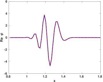
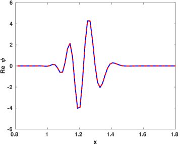
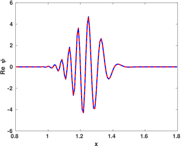
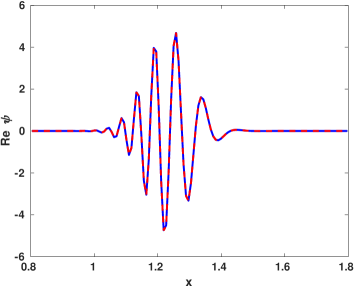
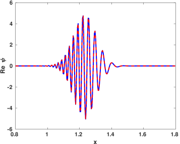
Firstly, we plot the real part of the wave function obtained using FGA in comparison with the reference solution in Figure 4.1 for different combinations of and . Specifically, we consider and . To assess the accuracy of FGA, Table 1 presents the errors between the FGA solutions and the corresponding reference solutions, i.e. , , for a wider range of parameter values, including and . Notably, the results demonstrate that FGA solutions provide a reliable approximation for the fractional Schrödinger equation, exhibiting the desired convergence with respect to .
(a)
(b)
(c)
(d)
(e)
(f)
Figure 4.1: The comparison for the real part of the reference solution (solid line) and the solution by FGA (dashed line) with different combinations of and in Example 1.
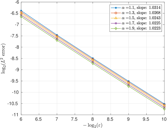
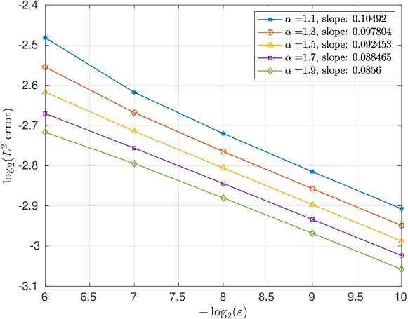
Now we turn to the convergence rate with respect to . Note that our chosen values of are all exponential powers of , to analyze the convergence behavior, we take the base-2 logarithm of both the errors of FGA solutions compared to the reference solutions and the corresponding values. By doing so, we obtain the decay curves of with respect to for each in the range of in Figure 4.2, where we employ the least square method to determine the slope of these curves. In the first subfigure of Figure 4.2, we set , while in the second subfigure, we use , which comes from the proof of the convergence theorem 1. Remarkably, in the scenario, the FGA displays a linear decay rate for the errors, which is consistent with the convergence rate observed for the standard Schrödinger equation. While in the scenario, one can observe that the logarithm of error decays at a slower rate, which indicates that the FGA solution converges, but the inequality bound in our proof is not very tight, leaving room for further improvement. Despite this suboptimal choice for , FGA exhibits desirable numerical properties and convergence rates for practical problems.
(a)
(b)
Figure 4.2: error decay behavior of FGA solution with different values in Example 1.
4.2 Two dimension
Example 2.
The initial condition is taken as
(4.3)
We solve the equation on domain with final time , under potential
(4.4)
In this example, we follow the same discussion in Example 1 to show the numerical behavior of FGA in the two-dimensional scenario. We take and , for the meshes of FGA with time step for solving the ODEs with -th order Runge-Kutta method. The reference solution is computed by the time-splitting spectral method with mesh sizes of and time step .
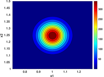
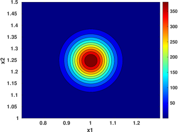
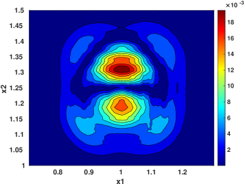
Figure 4.3 compares the wave amplitude of the FGA solution and the reference for and . The errors between these two solutions with a wider range of parameter values including and are given in Table 2. We can observe the accuracy of the FGA solution in two dimensions from these results.
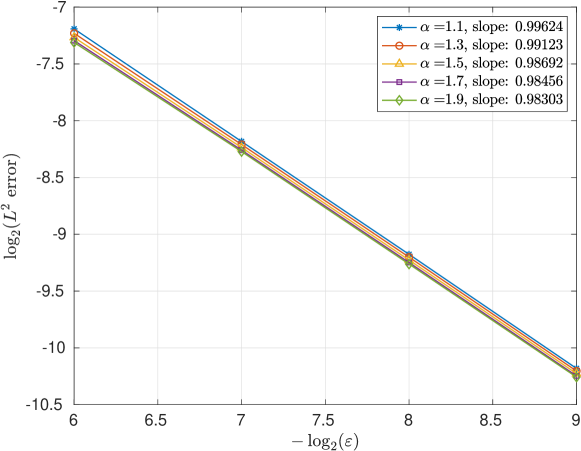
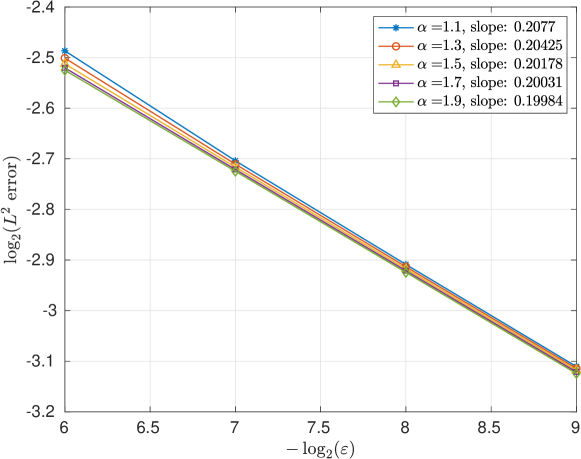
Furthermore, we plot the decay curves of with respect to for each in Figure 4.4. Again, the first subfigure uses and the second one uses , which is derived from our proof for the convergence theorem 1. Similar to the example in one dimension, the scenario displays a linear convergence rate, while the gives a slower decay rate.
(a)Frozen Gaussian approximation,
(b)Frozen Gaussian approximation,
(c)Reference solution,
(d)Reference solution,
(e)Errors,
(f)Errors,
Figure 4.3: The comparison of the wave amplitude of the reference solution and the solution by FGA with different values of and in Example 2.
Figure 4.4: error decay behavior of FGA solution in Example 2.
5 Conclusion and discussion
check grammar In this work, we propose the frozen Gaussian approximation (FGA) for computing the fractional Schrödinger equation in the semiclassical regime. This approach is based on asymptotic analysis and constructs the solution using Gaussian functions with fixed widths that live on the phase space. We develop a modified FGA formulation with a regularization parameter to address the presence of singularities in higher derivatives of the associated Hamiltonian flow. Our primary focus is on deriving formulations and establishing the rigorous convergence result for FGA. Additionally, we verify the accuracy of the FGA solutions through several numerical examples and demonstrate the method’s linear convergence rate with respect to .
There are several directions to extend and improve the work. Firstly, in the convergence proof for high-dimensional scenarios, it should be noted that the singularities arising from can be removed by the integral, similar to what is demonstrated in Lemma 5. Although the singularities in the higher derivative of FGA quantities, including , do not explicitly take the form with a constant , they should be removable through high dimensional integration with . We emphasize that, under certain assumptions, if one has the following estimate:
(5.1)
then it allows us to combine the singularity order of higher derivative of FGA quantities such as within into and to remove them by high dimensional integration to achieve favorable convergence order.
Secondly, to provide a rigorous convergence proof, we utilize the approximation chain
which establishes a relation between parameter and . However, the numerical results indicate the potential to relax such constraints, since the singularities do not appear in the integral representation of FGA. Finally, in this work, we employ the directed perturbation method to address the singularities and formulate the modified version of conventional FGA. It is worth noting that utilizing other methods to handle the singularities may lead to another type of modified FGA with a linear convergence rate.
Acknowledgements
L.C. was partially supported by
the National Key R&D Program of China No.2021YFA1003001,and the NSFC Projects No. 12271537 and 11901601. X.Y. was partially supported by the NSF grant DMS-2109116.
Firstly we prove the local existence and uniqueness of the solution for Hamiltonian equations (2.2). Our approach follows the spirit of the well known Picard successive approximation method.
Consider a small rectangular region defined as
Notice that when , we can always find small enough to make sure that for any , one has . Hence are smooth functions over region and satisfy the Lipschitz condition, which guarantees the local existence and uniqueness of solutions over . On the other hand, the Hamiltonian equations (2.2) will have unique constant solution, when and . Therefore, in the following, we may assume that
Without loss of generality, we might let and only consider the case when for a clearer proof. The other cases can be handled similarly.
Now let us introduce some more notations for the proof. Denote region
Since , with being the dimensional identity matrix, we have
(A.1)
where is a constant. Denote
and , where is a constant small enough such that
(A.2)
Now we define ,
(A.3)
(A.4)
Then by induction one can easily see that for , are continuous over and satisfy conditions
(A.5)
Furthermore, we claim that function sequences , are uniformly convergent over , i.e. , we will show that series
(A.6)
are uniformly convergent. To attain this, note that
where for the last inequality we use that for and .
Next, we use induction to prove that
(A.11)
and
(A.12)
We have already proved the case when , serves as the starting point of induction. Further, using the assumption of induction we have
then
Notice that for where satisfying
we have
(A.13)
Hence, for any ,
(A.14)
Finally, we have
where and
Therefore, together with and , one obtains
which completes the induction.
Now we come back to the local existence and uniqueness of the solution over region . For existence, since series
are convergent, are uniformly convergent. Taking limitation of (A.3), (A.4) with respect to , we get the solutions of Hamiltonian equations (2.2).
For uniqueness, suppose are another continuous solutions of Hamiltonian equations defined on , we claim that are also uniformly convergent limitation of respectively. In the same manner as the previous proof for local existence, we have
(A.15)
Note that the right-hand sides above approach to when , hence , which illustrates the local uniqueness.
Finally, after extending the local unique solution to a wider domain, we complete the proof of the existence and uniqueness of the solution of the Hamiltonian equations (2.2).
The proof of the existence and uniqueness of the solution to the Hamiltonian equation (2.2) with the modified kinetic symbol can be carried out in a similar manner as that for the original equation, with the only difference being the replacement of with . Notice that by taking the limit of (A.14) with respect to we obtain
Below, we will find a lower bound for that is independent of and by analyzing the derivation of (A.14) carefully.
Again, consider the region
Since , with being the dimensional identity matrix, we have
where is a constant independent with . Denote
then are constants independent with and . Besides, according to Proposition 3, we have
where is a constant independent of and . Hence,
On the other hand, for ,
Given a constant such that , it implies that
which is exactly the constraint (A.2) with being independent with and . Therefore, we can define such that is a constant independent with and . Then following the same argument to derive (A.14) we obtain,
By taking the limit with respect to , we obtain for , where and are independent of and . This completes the proof.
References
[1]
X. Antoine, E. Lorin, and Y. Zhang.
Derivation and analysis of computational methods for fractional
Laplacian equations with absorbing layers.
Numerical Algorithms, 87(1):409–444, May 2021.
[2]
X. Antoine, Q. Tang, and Y. Zhang.
On the ground states and dynamics of space fractional nonlinear
Schrödinger/Gross–Pitaevskii equations with rotation term and
nonlocal nonlinear interactions.
Journal of Computational Physics, 325:74–97, November 2016.
[3]
W. Bao, S. Jin, and P. A. Markowich.
On time-splitting spectral approximations for the schrödinger
equation in the semiclassical regime.
Journal of Computational Physics, 175(2):487–524, 2002.
[4]
R. Carles.
Semi-classical analysis for nonlinear Schrodinger equations.
World Scientific, 2008.
[5]
L. Chai, J. C. Hateley, E. Lorin, and X. Yang.
On the convergence of frozen Gaussian approximation for linear
non-strictly hyperbolic systems.
Comm. Math. Sci., 19(3):585–606, 2021.
[6]
L. Chai, E. Lorin, and X. Yang.
Frozen Gaussian approximation for the Dirac equation in
semi-classical regime.
SIAM J. Num. Anal., 57:2383–2412, 2019.
[7]
S. Duo and Y. Zhang.
Mass-conservative fourier spectral methods for solving the fractional
nonlinear schrödinger equation.
Computers & Mathematics with Applications, 71(11):2257–2271,
2016.
[8]
B. Engquist and O. Runborg.
Computational high frequency wave propagation.
Acta Numer., 12:181–266, 2003.
[9]
J. Fröhlich, B. L. G. Jonsson, and E. Lenzmann.
Boson stars as solitary waves.
Communications in mathematical physics, 274(1):1–30, 2007.
[10]
P. Gérard, P. A. Markowich, N. J. Mauser, and F. Poupaud.
Homogenization limits and wigner transforms.
Communications on Pure and Applied Mathematics: A Journal Issued
by the Courant Institute of Mathematical Sciences, 50(4):323–379, 1997.
[11]
L. Gosse, S. Jin, and X. Li.
Two moment systems for computing multiphase semiclassical limits of
the schrödinger equation.
Mathematical Models and Methods in Applied Sciences,
13(12):1689–1723, 2003.
[12]
G. A. Hagedorn.
Raising and lowering operators for semiclassical wave packets.
Annals of Physics, 269(1):77–104, 1998.
[13]
J. C. Hateley, L. Chai, P. Tong, and X. Yang.
Frozen Gaussian approximation for 3-D elastic wave equation and
seismic tomography.
Geophysical Journal International, 216(2):1394–1412, 2019.
[14]
E. J. Heller.
Frozen Gaussians: A very simple semiclassical approximation.
J. Chem. Phys., 75:2923–2931, 1981.
[15]
M. F. Herman and E. Kluk.
A semiclassical justification for the use of non-spreading
wavepackets in dynamics calculations.
Chem. Phys., 91:27–34, 1984.
[16]
L. Hörmander and L. Hörmander.
The analysis of linear partial differential operators. III:
Pseudo-Differential Operators.
Springer-Verlag, 1994.
[17]
Y. Huang and A. Oberman.
Numerical methods for the fractional laplacian: A finite
difference-quadrature approach.
SIAM Journal on Numerical Analysis, 52(6):3056–3084, 2014.
[18]
Z. Huang, L. Xu, and Z. Zhou.
Efficient frozen Gaussian sampling algorithms for nonadiabatic
quantum dynamics at metal surfaces.
ArXiv, abs/2206.02173, 2022.
[19]
S. Jin, P. Markowich, and C. Sparber.
Mathematical and computational methods for semiclassical
schrödinger equations.
Acta Numerica, 20:121–209, 2011.
[20]
K. Kay.
Integral expressions for the semi-classical time-dependent
propagator.
J. Chem. Phys., 100:4377–4392, 1994.
[21]
K. Kay.
The Herman-Kluk approximation: Derivation and semiclassical
corrections.
Chem. Phys., 322:3–12, 2006.
[22]
K. Kirkpatrick and Y. Zhang.
Fractional Schrödinger dynamics and decoherence.
Physica D: Nonlinear Phenomena, 332:41–54, 2016.
[23]
C. Klein, C. Sparber, and P. Markowich.
Numerical study of fractional Nonlinear
Schr\”odinger equations.
Proceedings of the Royal Society A: Mathematical, Physical and
Engineering Sciences, 470(2172):20140364, December 2014.
arXiv:1404.6262 [math].
[24]
N. Laskin.
Fractional quantum mechanics.
Physical Review E, 62(3):3135, 2000.
[25]
N. Laskin.
Fractional Schrödinger equation.
Physical Review E, 66(5):056108, 2002.
[26]
N. Laskin.
Fractional quantum mechanics and Lévy path integrals.
Physics Letters A, 268(4-6):298–305, 2000.
[27]
C. Lasser and D. Sattlegger.
Discretising the herman–kluk propagator.
Numerische Mathematik, 137, 09 2017.
[28]
E. Lenzmann.
Well-posedness for semi-relativistic hartree equations of critical
type.
Mathematical Physics, Analysis and Geometry, 10(1):43–64,
2007.
[29]
P.-L. Lions and T. Paul.
Sur les mesures de wigner.
Revista matemática iberoamericana, 9(3):553–618, 1993.
[30]
J. Lu and X. Yang.
Frozen Gaussian approximation for high frequency wave propagation.
Commun. Math. Sci., 9:663–683, 2011.
[31]
J. Lu and X. Yang.
Convergence of frozen Gaussian approximation for high frequency
wave propagation.
Comm. Pure Appl. Math., 65:759–789, 2012.
[32]
J. Lu and Z. Zhou.
Improved sampling and validation of frozen Gaussian approximation
with surface hopping algorithm for nonadiabatic dynamics.
J Chem Phys., 145(12):124109, 2016.
[33]
J. Lu and Z. Zhou.
Frozen Gaussian approximation with surface hopping for mixed
quantum-classical dynamics: A mathematical justification of fewest switches
surface hopping algorithms.
Math. Comput., 87:2189–2232, 2018.
[34]
C. Lubich.
On splitting methods for schrödinger-poisson and cubic nonlinear
schrödinger equations.
Mathematics of computation, 77(264):2141–2153, 2008.
[35]
A. Martinez.
An introduction to semiclassical and microlocal analysis,
volume 994.
Springer, 2002.
[36]
T. Swart and V. Rousse.
A mathematical justification of the Herman-Kluk propagator.
Commun. Math. Phys., 286:725–750, 2009.
[37]
L. Tartar.
H-measures, a new approach for studying homogenisation, oscillations
and concentration effects in partial differential equations.
Proceedings of the Royal Society of Edinburgh Section A:
Mathematics, 115(3-4):193–230, 1990.
[38]
W. Wang, Y. Huang, and J. Tang.
Lie-trotter operator splitting spectral method for linear
semiclassical fractional schrödinger equation.
Computers & Mathematics with Applications, 113:117–129, 2022.