Differentially Private Distributed Nonconvex Stochastic Optimization with Quantized Communications

Abstract

This paper proposes a new distributed nonconvex stochastic optimization algorithm that can achieve privacy protection, communication efficiency and convergence simultaneously. Specifically, each node adds time-varying privacy noises to its local state to avoid information leakage, and then quantizes its noise-perturbed state before transmitting to improve communication efficiency. By employing the subsampling method controlled through the sample-size parameter, the proposed algorithm reduces the impact of privacy noises, and enhances the differential privacy level. When the global cost function satisfies the Polyak-Łojasiewicz condition, the mean and high-probability convergence rate and the oracle complexity of the proposed algorithm are given. Importantly, the proposed algorithm achieves both the mean convergence and a finite cumulative differential privacy budget over infinite iterations as the sample-size goes to infinity. A numerical example of the distributed training on the “MNIST” dataset is given to show the effectiveness of the algorithm.

Differential privacy, distributed stochastic optimization, probabilistic quantization.

1 Introduction

Distributed optimization is gaining more and more attraction due to its fundamental role in cooperative control, distributed sensing, sensor networks, and large-scale machine learning. In many of these applications, the problem can be formulated as a network of nodes cooperatively solve a common optimization problem through on-node computation and local communication [1, 2, 6, 3, 4, 5, 7, 8, 9, 10, 11]. As a branch of distributed optimization, distributed stochastic optimization focuses on finding optimal solutions for stochastic cost functions in a distributed manner. For example, distributed stochastic gradient descent (SGD) [6, 7], distributed SGD with quantized communication [8], SGD with gradient compression [9, 10], and distributed SGD with variable sample method [11] are given, respectively.

When nodes exchange information to solve a distributed stochastic optimization problem, there are two issues worthy of attention. One is the leakage of the sensitive information concerning cost functions, and the other is the network bandwidth limitation. To solve the first issue, it is necessary to design some privacy-preserving techniques to protect the privacy in distributed stochastic optimization [12]. So far, various techniques have been employed to prevent information leakage, such as homomorphic encryption [13], correlated noise based approach [14], structure techniques [15, 16, 17], differential privacy [19, 18, 20, 21, 22, 23] and so on. Homomorphic encryption often incurs a communication and computation burden, while correlated noise based approach and structure techniques provide only limited privacy protection. Due to its simplicity and wide applicability in privacy protection, differential privacy has attracted a lot of attention and been used to solve the privacy issues in distributed optimization. For example, distributed stochastic optimization algorithms with differential privacy are proposed in [24, 25, 26, 27, 29, 32, 31, 30, 28]. In distributed convex stochastic optimization with differential privacy, distributed SGD with output perturbation [24], alternating direction method of multipliers with output perturbation [25], distributed SGD with quantized communication [26], zeroth-order alternating direction method of multipliers with output perturbation [27], and distributed dual averaging with gradient perturbation [28] are given, respectively. In distributed nonconvex stochastic optimization, distributed SGD with gradient perturbation [29, 30] and quantization enabled privacy protection [31, 32] are given, respectively. However, to prove the convergence and the differential privacy, the assumption of bounded gradients is required in [10, 24, 25, 26, 27, 31, 30, 28]. Besides, differential privacy is only given for each iteration in [24, 25, 26, 27, 29, 31, 30, 32, 28], leading to an infinite cumulative differential privacy budget over infinite iterations.

To solve the second issue, a common method for each node is to transmit quantized information instead of the raw information. The examples include the adaptive quantization [3] and the probabilistic quantization [26, 31, 32, 9]. However, to the best of our knowledge, there is still no algorithm that can achieve privacy protection, communication efficiency and convergence simultaneously in distributed nonconvex stochastic optimization. Therefore, this paper will focus on how to design a privacy-preserving distributed nonconvex stochastic optimization algorithm that can enhance the differential privacy level while achieving communication efficiency and convergence simultaneously; and show how the added privacy noises and the quantization error affect the convergence rate of the algorithm.

The main contributions of this paper are as follows:

• Differential privacy, communication efficiency and convergence of the proposed algorithm are considered simultaneously. By employing the subsampling method controlled through the sample-size parameter, the proposed algorithm can enhance the differential privacy with guaranteed mean convergence even for increasing privacy noises.

• The convergence rate for more general privacy noise cases is provided, which includes the noises with either constant or increasing variance. Under the Polyak-Łojasiewicz condition, the mean and high-probability convergence rate of the proposed algorithm are given without requiring the gradients are bounded.

• When the sample-size goes to infinity, the algorithm achieves both the mean convergence and a finite cumulative differential privacy budget over infinite iterations.

The results in this paper are significantly different from those in existing works. A comparison with the state-of-the-art is as follows: Compared with [24, 25, 26, 27, 29, 31, 30, 32, 28], the differential privacy level is enhanced, and a finite cumulative differential privacy budget is achieved over infinite iterations. Compared with [7, 25, 26, 31, 30, 28], the convergence of the proposed algorithm is given without requiring the gradients are bounded. Compared with [10, 27, 9, 32], the convergence is achieved. Compared with [6, 8, 9, 10, 24, 25, 27, 11, 29, 30, 28, 31, 26, 32], the high-probability convergence rate is given to show the effectiveness of the algorithm. Compared with [6, 8, 9, 10, 7, 24, 25, 27, 11, 29, 30, 28], privacy protection and communication efficiency are considered simultaneously in this paper.

This paper is organized as follows: Section 2 formulates the problem to be investigated. Section 3 presents the main results including the privacy, convergence and oracle complexity analysis of the algorithm. Section 4 provides a numerical example of the distributed training of a convolutional neural network on the “MNIST” dataset. Section 5 gives some concluding remarks.

Notation: $\mathbb{R}$ and $\mathbb{R}^{d}$ denote the set of all real numbers and $d$-dimensional Euclidean space, respectively. $\mathrm{Range}(F)$ denotes the range of a mapping $F$, and $F\circ G$ denotes the composition of mappings $F$ and $G$. For sequences $\{a_{k}\}_{k=1}^{\infty}$ and $\{b_{k}\}_{k=1}^{\infty}$, $a_{k}=O(b_{k})$ means there exists $A_{1}\geq 0$ such that $\limsup_{k\to\infty}|\frac{a_{k}}{b_{k}}|\leq A_{1}$. $\mathbf{1}_{n}$ represents an $n$-dimensional vector whose elements are all 1. $A^{\top}$ stands for the transpose of the matrix $A$. We use the symbol $\|x\|=\sqrt{x^{\top}x}$ to denote the standard Euclidean norm of $x=[x_{1},x_{2},\dots,x_{m}]^{\top}$, and $\|A\|$ to denote the 2-norm of the matrix $A$. $\mathbb{P}(\mathcal{B})$ and $\mathbb{E}(X)$ refers to the probability of an event $\mathcal{B}$ and the expectation of a random variable $X$, respectively. $\otimes$ denotes the Kronecker product of matrices. $\lfloor z\rfloor$ denotes the largest integer no larger than $z$. For a vector $v=[v_{1},v_{2},\dots,v_{n}]^{\top}$, $\textrm{diag}(v)$ denotes the diagonal matrix with diagonal elements being $v_{1},v_{2},\dots,v_{n}$. For a differentiable function $f(x)$, $\nabla f(x)$ denotes its gradient at the point $x$.

2 Preliminaries and problem formulation

2.1 Graph theory

Consider a network of $n$ nodes, whose communication graph is denoted by $\mathcal{G}=(\mathcal{V},\mathcal{E},\mathcal{A})$. $\mathcal{V}=\{1,2,\dots,n\}$ is the set of all nodes, and $\mathcal{E}$ stands for the set of all edges. An edge $e_{ij}\in\mathcal{E}$ if and only if Node $i$ can receive the information from $j$. The entry $a_{ij}$ of the adjacency matrix $\mathcal{A}=\left(a_{ij}\right)_{1\leq i,j\leq n}$ is either strictly positive if $e_{ij}\in\mathcal{E}$, or 0, otherwise. The neighbor set of Node $i$ is defined as $\mathcal{N}_{i}=\{j\in\mathcal{V}:a_{ij}>0\}$, and the Laplacian matrix of $\mathcal{A}$ is defined as $\mathcal{L}=\textrm{diag}(\mathcal{A}\mathbf{1}_{n})-\mathcal{A}$. The assumption about the communication graph $\mathcal{G}$ is given as follows:

Assumption 1

The undirected communication graph $\mathcal{G}$ is connected, and the adjacency matrix $\mathcal{A}$ is doubly stochastic, i.e., $\mathcal{A}\mathbf{1}_{n}=\mathbf{1}_{n}$, $\mathbf{1}_{n}^{\top}\mathcal{A}=\mathbf{1}_{n}^{\top}$.

2.2 Distributed stochastic optimization

In this paper, the following distributed nonconvex stochastic optimization problem is considered:

$$\min_{x\in\mathbb{R}^{d}}\!F(x)\!=\!\min_{x\in\mathbb{R}^{d}}\!\frac{1}{n}\!\sum_{i=1}^{n}\!f_{i}(x),f_{i}(x)\!=\!\mathbb{E}_{\xi_{i}\sim D_{i}}[\ell_{i}(x,\xi_{i})],$$ (1)

where $x$ is available to all nodes, $\ell_{i}(x,\xi_{i})$ is a local cost function which is private to Node $i$, and $\xi_{i}$ is a random variable drawn from an unknown probability distribution $D_{i}$. In practice, since the probability distribution $D_{i}$ is difficult to obtain, it is replaced by the dataset $\mathcal{D}_{i}=\{\xi_{i,1},\xi_{i,2},\dots,\xi_{i,D}\}$. Then, (1) can be rewritten as the following empirical risk minimization problem:

$$\min_{x\in\mathbb{R}^{d}}\!F(x)\!=\!\min_{x\in\mathbb{R}^{d}}\!\frac{1}{n}\!\sum_{i=1}^{n}\!f_{i}(x),f_{i}(x)\!=\!\frac{1}{D}\sum_{j=1}^{D}\ell_{i}(x,\xi_{i,j}).$$ (2)

To solve the problem (2), we need the following assumption.

Assumption 2

The following conditions on the cost functions hold:

1. For any node $i\in\mathcal{V}$, $f_{i}$ has Lipschitz continuous gradients, i.e.,

   $$\|\nabla f_{i}(x)-\nabla f_{i}(y)\|\leq L\|x-y\|,\forall x,y\in\mathbb{R}^{d},$$

   where $L$ is a positive constant.

2. Each cost function and their sum are bounded from below, i.e.,

   $$\min_{x\in\mathbb{R}^{d}}\!F(x)\!=\!F^{*}\!>\!-\infty,\min_{x\in\mathbb{R}^{d}}\!f_{i}(x)\!=\!f_{i}^{*}\!>\!-\infty.$$

3. For any node $i\in\mathcal{V},x\in\mathbb{R}^{d}$ and $\zeta_{i}$ uniformly sampled from $\mathcal{D}_{i}$, there exists a stochastic first-order oracle which returns a sampled gradient $g_{i}(x,\zeta_{i})$ of $f_{i}(x)$. In addition, there exists $\sigma_{g}>0$ such that each sampled gradient $g_{i}(x,\zeta_{i})$ satisfies

   $$\mathbb{E}[g_{i}(x,\zeta_{i})]=\nabla f_{i}(x),$$

   $$\mathbb{E}[\|g_{i}(x,\zeta_{i})-\nabla f_{i}(x)\|^{2}]\leq\sigma_{g}^{2}.$$

4. (Polyak-Łojasiewicz) There exists $\mu>0$ such that

   $$2\mu(F(x)-F^{*})\leq\|\nabla F(x)\|^{2},\forall x\in\mathbb{R}^{d}.$$

Remark 1

Assumption 2(i) is standard and commonly used (see e.g. [8, 11, 26, 5, 29, 7, 32, 31, 30]). Assumption 2(ii) ensures the existence of the solution. Assumption 2(iii) is standard and commonly used (see e.g. [11, 26, 29, 31, 32]). It means each sampled gradient $g_{i}(x,\xi_{i}^{l})$ is unbiased with a bounded variance $\sigma_{g}^{2}$. Assumption 2(iv) is standard and commonly used (see e.g. [5, 33]). It requires the gradient $\nabla F(x)$ to grow faster than a quadratic function as the algorithm moves away from the optimal solution. This kind of functions exists, for example, $F(x)=x^{2}+3\sin^{2}x$ is a nonconvex function satisfying Assumption 2(iv) for any $0<\mu<0.3$. As shown in Theorem 2 of [34], Assumption 2(iv) is weaker than the convex cost functions assumed in [11, 24, 25, 8, 26, 27, 28].

2.3 Quantized communication

To improve communication efficiency of the algorithm, a probabilistic quantizer is used to quantize the exchanged information. The probabilistic quantizer is a randomized mapping that maps an input to different values in a discrete set with some probability distribution. In this paper, we consider the probabilistic quantizers satisfying the following assumption:

Assumption 3

The probabilistic quantizer $Q(x)$ is unbiased and its variance is bounded, which means there exists $\Delta>0$, such that $\mathbb{E}(Q(x)|x)=x$ and $\mathbb{E}(|Q(x)\!-\!x|^{2}|x)\!\leq\!\Delta^{2}$.

Remark 2

Assumption 3 is standard and commonly used (see e.g. [8, 26]). Here is an example: Given $\Delta>0$, the quantizer $Q(x)$ with the following probability distribution satisfies Assumption 3 by Lemma 1 of [35].

$$\begin{cases}\mathbb{P}\left(\left.Q(x)=\Delta\lfloor\frac{x}{\Delta}\rfloor\right|x\right)=1-\frac{x}{\Delta}+\lfloor\frac{x}{\Delta}\rfloor;\cr\mathbb{P}\left(\left.Q(x)=\Delta\left(\lfloor\frac{x}{\Delta}\rfloor+1\right)\right|x\right)=\frac{x}{\Delta}-\lfloor\frac{x}{\Delta}\rfloor.\end{cases}$$ (3)

2.4 Differential privacy

As shown in [12, 21, 28, 31, 30], there are two kinds of adversary models widely used in the privacy-preserving issue:

• A semi-honest adversary. This kind of adversary is defined as a node within the network which has access to certain internal states (such as $x_{i,k}$ from Node $i$), follows the prescribed protocols and accurately computes iterative state correctly. However, it aims to infer the sensitive information of other nodes.

• An eavesdropper. This kind of adversary refers to an external adversary who has capability to wiretap and monitor all communication channels, allowing them to capture distributed messages from any node. This enables the eavesdropper to infer sensitive information of the internal nodes.

When solving the problem (2), the stochastic first-order oracle needs data samples to return sampled gradients. Meanwhile, the adversaries can infer sensitive information of data samples from the change of sampled gradients (​​[36]). In order to provide privacy protection for data samples, inspired by [21, 28], a symmetric binary relation called adjacency relation is defined as follows:

Definition 1

(Adjacency relation) For any fixed node $i\in\mathcal{V}$, let $\mathcal{D}=\{\xi_{i,l},1\leq l\leq D\},\mathcal{D}^{\prime}=\{\xi_{i,l}^{\prime},1\leq l\leq D\}$ be two sets of data samples. If for a given $C>0$ and any $x\in\mathbb{R}^{d}$, there exists exactly one pair of data samples $\xi_{i,l_{0}},\xi_{i,l_{0}}^{\prime}$ in $\mathcal{D},\mathcal{D}^{\prime}$ such that

$$\begin{cases}\!\|g_{i}(x,\xi_{i,l})\!-\!g_{i}(x,\xi_{i,l}^{\prime})\|\!\leq\!C,&\mathrm{if}\;l=l_{0};\cr\!\|g_{i}(x,\xi_{i,l})\!-\!g_{i}(x,\xi_{i,l}^{\prime})\|\!=\!0,&\mathrm{if}\;l\neq l_{0},\end{cases}\!\!\!\!$$ (4)

then $\mathcal{D}$ and $\mathcal{D}^{\prime}$ are said to be adjacent, denoted by $\mathrm{Adj}(\mathcal{D},\mathcal{D}^{\prime})$.

Remark 3

From Definition 1, it follows that $\mathcal{D}$ and $\mathcal{D}^{\prime}$ are adjacent if exactly one pair of data samples $\xi_{i,l_{0}},\xi_{i,l_{0}}^{\prime}$ in $\mathcal{D},\mathcal{D}^{\prime}$ satisfies $\|g_{i}(x,\xi_{i,l_{0}})-g_{i}(x,\xi_{i,l_{0}}^{\prime})\|\!\leq\!C$ and the others satisfy $\|g_{i}(x,\xi_{i,l})-g_{i}(x,\xi_{i,l}^{\prime})\|\!=\!0$ if $l\neq l_{0}$ for any $x\in\mathbb{R}^{d}$.

To give the privacy-preserving level of the algorithm, we adopt the definition of $(\epsilon,\delta)$-differential privacy as follows:

Definition 2

​​[28] (Differential privacy) Given $\epsilon,\delta>0$, a randomized algorithm $\mathcal{M}$ is $(\epsilon,\delta)$-differentially private for $\mathrm{Adj}(\mathcal{D},\mathcal{D}^{\prime})$ if for any subset $T\subset\mathrm{Range}(\mathcal{M})$, it holds that

$$\mathbb{P}(\mathcal{M}(\mathcal{D})\in T)\leq e^{\epsilon}\mathbb{P}(\mathcal{M}(\mathcal{D}^{\prime})\in T)+\delta.$$

Lemma 1

​​[19] (Post-processing) Let $\mathcal{M}$ be a randomized algorithm that is $(\epsilon,\delta)$-differentially private for $\mathrm{Adj}(\mathcal{D},\mathcal{D}^{\prime})$, and $Q$ a randomized mapping defined on $\mathrm{Range}(\mathcal{M})$. Then, $Q\circ\mathcal{M}$ is $(\epsilon,\delta)$-differentially private for $\mathrm{Adj}(\mathcal{D},\mathcal{D}^{\prime})$.

3 Main result

3.1 The proposed algorithm

In this subsection, we give a differentially private distributed nonconvex stochastic optimization algorithm with quantized communication. The detailed implementation steps are given in Algorithm 1.

Algorithm 1 Differentially private distributed nonconvex stochastic optimization algorithm with quantized communication

1:$x_{i,0}\in\mathbb{R}^{d}$ for any node $i\in\mathcal{V}$, weight matrix $(a_{ij})_{1\leq i,j\leq n}$, iteration limit $K$, step-sizes $\hat{\alpha}$, $\hat{\beta}$ and sample-size $\hat{\gamma}$. for $k=0,1,2,\dots,K$, do

2:Node $i$ adds noise $n_{i,k}$ to $x_{i,k}$ and computes the quantized information $z_{i,k}=Q(x_{i,k}+n_{i,k})=[Q(x_{i,k}^{(1)}+n_{i,k}^{(1)}),\dots,Q(x_{i,k}^{(d)}+n_{i,k}^{(d)})]^{\top}$ with the probabilistic quantizer in the form of (3), where $n_{i,k}\sim N(0,\sigma_{k}^{2}I_{d})$.

3:Node $i$ broadcasts $z_{i,k}$ to its neighbors $j\in\mathcal{N}_{i}$.

4:Node $i$ receives $z_{j,k}$ from its neighbors $j\in\mathcal{N}_{i}$, and takes $\hat{\gamma}$ data samples $\{\zeta_{i,k,1},\zeta_{i,k,2},\dots,\zeta_{i,k,\hat{\gamma}}\}$ uniformly from $\mathcal{D}_{i}$ without replacement to generate

$$g_{i,k}=\frac{1}{\hat{\gamma}}\sum_{l=1}^{\hat{\gamma}}g_{i}(x_{i,k},\zeta_{i,k,l}).$$ (5)

5:Node $i$ updates its state via

$$x_{i,k+1}\!=\!(1\!-\!\hat{\beta})x_{i,k}\!+\!\hat{\beta}\!\sum_{j\in\mathcal{N}_{i}}\!\!a_{ij}z_{j,k}\!-\!\hat{\alpha}g_{i,k}.$$ (6)

end for

3.2 Privacy analysis

In the following, we will show the differential privacy analysis of Algorithm 1. Inspired by [21], we provide the sensitivity of the algorithm, which helps us to analyze the cumulative differential privacy budget of the algorithm.

Definition 3

(Sensitivity) Given two groups of adjacent sample sets $\mathcal{D},\mathcal{D}^{\prime}$, and a mapping $q$. For any $0\leq k\leq K$, let $\hat{\gamma}$ be the number of taken data samples at the $k$-th iteration, and $\mathcal{D}_{k}=\{\zeta_{i,k,l},1\leq l\leq\hat{\gamma}\},\mathcal{D}_{k}^{\prime}=\{\zeta_{i,k,l}^{\prime},1\leq l\leq\hat{\gamma}\}$ the data samples taken from $\mathcal{D},\mathcal{D}^{\prime}$ at the $k$-th iteration, respectively. Define the sensitivity of $q$ at the $k$-th iteration of Algorithm 1, denoted by $\Delta_{k}$, as follows:

$$\Delta_{k}\triangleq\sup_{\mathrm{Adj}(\mathcal{D},\mathcal{D}^{\prime})}\|q(\mathcal{D}_{k})-q(\mathcal{D}_{k}^{\prime})\|.$$ (7)

Remark 4

Definition 3 captures the magnitude by which a single individual’s data can change the mapping $q$ in the worst case. It is the key quantity showing how many noises should be added to achieve $(\epsilon,\delta)$-differential privacy at the $k$-th iteration. In Algorithm 1, the mapping $q(\mathcal{D}_{k})=x_{i,k+1}$, the randomized algorithm $\mathcal{M}(\mathcal{D}_{k})=x_{i,k+1}+n_{i,k+1}$, and the randomized mapping $Q(\mathcal{M}(\mathcal{D}_{k}))=z_{i,k+1}$, since the quantizer $Q$ is of the form (3).

The following lemma gives the sensitivity $\Delta_{k}$ of the proposed algorithm for any $0\leq k\leq K$.

Lemma 2

At the $k$-th iteration, the sensitivity of the proposed algorithm satisfies

$$\Delta_{k}\leq\frac{\hat{\alpha}C}{\hat{\gamma}}\left(\sum_{m=0}^{k}|1-\hat{\beta}|^{m}\right).$$

Proof: When $k=0$, substituting (6) into (7) results in

$$\Delta_{0}= \sup_{\mathrm{Adj}(\mathcal{D},\mathcal{D}^{\prime})}\left\|q(\mathcal{D}_{0})-q(\mathcal{D}_{0}^{\prime})\right\|$$ (8)

$$= \sup_{\mathrm{Adj}(\mathcal{D},\mathcal{D}^{\prime})}\left\|x_{i,1}-x_{i,1}^{\prime}\right\|$$ (9)

$$= \sup_{\mathrm{Adj}(\mathcal{D},\mathcal{D}^{\prime})}\|(1-\hat{\beta})(x_{i,0}-x_{i,0}^{\prime})$$ (10)

$$+\hat{\beta}\sum_{j\in\mathcal{N}_{i}}a_{ij}(z_{j,0}-z_{j,0}^{\prime})-\hat{\alpha}(g_{i,0}-g_{i,0}^{\prime})\|.$$ (11)

Note that the initial value $x_{i,0}=x_{i,0}^{\prime}$, and the quantized information $z_{j,0}=z_{j,0}^{\prime}$ for any $j\in\mathcal{N}_{i}$. Then, (8) can be rewritten as

$$\Delta_{0}=\sup_{\mathrm{Adj}(\mathcal{D},\mathcal{D}^{\prime})}\left\|\hat{\alpha}(g_{i,0}-g_{i,0}^{\prime})\right\|.$$

This together with (5) gives

$$\Delta_{0}\!=\frac{\hat{\alpha}}{\hat{\gamma}}\!\!\sup_{\mathrm{Adj}(\mathcal{D},\mathcal{D}^{\prime})}\!\left\|\!\sum_{l=1}^{\hat{\gamma}}\!(g_{i}(x_{i,0},\zeta_{i,0,l})\!-\!g_{i}(x_{i,0},\zeta_{i,0,l}^{\prime}))\!\right\|\!.\!$$ (12)

By Definition 1, since $\mathcal{D},\mathcal{D}^{\prime}$ are adjacent, there exists exactly one pair of data samples $\xi_{i,l_{0}},\xi_{i,l_{0}}^{\prime}$ in $\mathcal{D},\mathcal{D}^{\prime}$ such that (4) holds. Then, there exists at most one pair of data samples $\zeta_{i,0,l_{1}},\zeta_{i,0,l_{1}}^{\prime}$ in (12) such that $\|g_{i}(x_{i,0},\zeta_{i,0,l_{1}})-g_{i}(x_{i,0},\zeta_{i,0,l_{1}}^{\prime})\|\leq C$, since $\hat{\gamma}$ data samples are taken uniformly from $\mathcal{D}$ without replacement. Hence, we have

$$\sup_{\mathrm{Adj}(\mathcal{D},\mathcal{D}^{\prime})}\!\left\|\!\sum_{l=1}^{\hat{\gamma}}(g_{i}(x_{i,0},\zeta_{i,0,l})-g_{i}(x_{i,0},\zeta_{i,0,l}^{\prime}))\right\|$$ (13)

$$\leq \sup_{\mathrm{Adj}(\mathcal{D},\mathcal{D}^{\prime})}\!\left\|g_{i}(x_{i,0},\zeta_{i,0,l_{1}})-g_{i}(x_{i,0},\zeta_{i,0,l_{1}}^{\prime})\right\|\leq C.$$ (14)

Thus, substituting (13) into (12) gives $\Delta_{0}\leq\frac{\hat{\alpha}}{\hat{\gamma}}C$.

When $1\leq k\leq K$, by (6) and (7) we have

$$\Delta_{k}= \sup_{\mathrm{Adj}(\mathcal{D},\mathcal{D}^{\prime})}\left\|x_{i,k+1}-x_{i,k+1}^{\prime}\right\|$$ (15)

$$= \sup_{\mathrm{Adj}(\mathcal{D},\mathcal{D}^{\prime})}\|(1-\hat{\beta})(x_{i,k}-x_{i,k}^{\prime})$$ (16)

$$+\hat{\beta}\sum_{j\in\mathcal{N}_{i}}a_{ij}(z_{j,k}-z_{j,k}^{\prime})-\hat{\alpha}(g_{i,k}-g_{i,k}^{\prime})\|.$$ (17)

Note that the quantized information $z_{j,k}=z_{j,k}^{\prime}$ for any $j\in\mathcal{N}_{i}$. Then, substituting (5) into (15) leads to

$$\!\!\Delta_{k}= \!\!\sup_{\mathrm{Adj}(\mathcal{D},\mathcal{D}^{\prime})}\|(1\!-\!\hat{\beta})(x_{i,k}\!-\!x_{i,k}^{\prime})\!-\!\hat{\alpha}(g_{i,k}\!-\!g_{i,k}^{\prime})\|$$ (18)

$$\leq \sup_{\mathrm{Adj}(\mathcal{D},\mathcal{D}^{\prime})}\!\!\|(1-\hat{\beta})(x_{i,k}-x_{i,k}^{\prime})\|$$ (19)

$$+\!\!\!\!\sup_{\mathrm{Adj}(\mathcal{D},\mathcal{D}^{\prime})}\!\!\left\|\!\frac{\hat{\alpha}}{\hat{\gamma}}\!\!\sum_{l=1}^{\hat{\gamma}}(g_{i}(x_{i,k},\zeta_{i,k,l})\!\!-\!\!g_{i}(x_{i,k},\zeta_{i,k,l}^{\prime})\!)\!\right\|\!\!.$$ (20)

Since $\mathcal{D},\mathcal{D}^{\prime}$ are adjacent, there exists at most one pair of data samples $\zeta_{i,k,l_{1}},\zeta_{i,k,l_{1}}^{\prime}$ such that $\|g_{i}(x_{i,k},\zeta_{i,k,l_{1}})-g_{i}(x_{i,k},\zeta_{i,k,l_{1}}^{\prime})\|\leq C$. Then, (18) can be rewritten as

$$\Delta_{k}\leq \sup_{\mathrm{Adj}(\mathcal{D},\mathcal{D}^{\prime})}\left\|(1-\hat{\beta})(x_{i,k}-x_{i,k}^{\prime})\right\|$$ (21)

$$+\frac{\hat{\alpha}}{\hat{\gamma}}\sup_{\mathrm{Adj}(\mathcal{D},\mathcal{D}^{\prime})}\left\|g_{i}(x_{i,k},\zeta_{i,k,l_{1}})-g_{i}(x_{i,k},\zeta_{i,k,l_{1}}^{\prime})\right\|$$ (22)

$$\leq |1-\hat{\beta}|\sup_{\mathrm{Adj}(\mathcal{D},\mathcal{D}^{\prime})}\left\|x_{i,k}-x_{i,k}^{\prime}\right\|+\frac{\hat{\alpha}C}{\hat{\gamma}}.$$ (23)

Therefore, by iteratively computing (21), this lemma is proved. $\blacksquare$

The following lemma is from Theorem A.1 in [19], which helps us to achieve $(\epsilon,\delta)$-differential privacy by the Gaussian mechanism.

Lemma 3

At the $k$-th iteration, given $0<\epsilon_{k}<1$, $\delta_{k}>0$, $c_{k}^{2}>2\ln\left(\frac{1.25}{\delta_{k}}\right)$ and the mapping $q$. For any subset $T^{(k)}\subset\mathbb{R}^{d}$, if sample sets $\mathcal{D}_{k}$ and $\mathcal{D}_{k}^{\prime}$ satisfy (4), then the Gaussian mechanism $\mathcal{M}(\mathcal{D}_{k})=q(\mathcal{D}_{k})+n_{i,k+1}$ satisfies

$$\mathbb{P}\!\left(\!\mathcal{M}(\mathcal{D}_{k})\!\in\!T^{(k)}\!\right)\!\leq e^{\epsilon_{k}}\!\mathbb{P}\!\left(\!\mathcal{M}(\mathcal{D}_{k}^{\prime})\in T^{(k)}\!\right)\!+\!\delta_{k},$$ (24)

where $n_{i,k+1}\sim N(0,\sigma_{k+1}^{2}I_{d})$ is a Gaussian noise with the variance $\sigma_{k+1}^{2}\geq(\frac{c_{k}\Delta_{k}}{\epsilon_{k}})^{2}$.

Theorem 1

For any $K\geq 2,0\leq k\leq K$, let

$$\hat{\alpha}=\frac{a_{1}(\ln K)^{2}}{K^{\alpha}},\quad\hat{\beta}=\frac{a_{2}}{K^{\beta}},\quad\hat{\gamma}=\lfloor a_{3}K^{\gamma}\rfloor+1,$$

$$\sigma_{k}=(k+1)^{\sigma},\quad\delta_{k}=\frac{1}{(k+1)^{\delta}},\quad c_{k}^{2}=4\ln(\frac{1.25}{\delta_{k}}),$$

$$a_{1},\ a_{2},\ a_{3}>0.$$

If $0<a_{2}<K^{\beta},\delta>0$, then Algorithm 1 is $(\epsilon,\hat{\delta})$-differentially private over finite iterations $K$, where

$$\epsilon \leq\sum_{k=0}^{K}\frac{2Ca_{1}a_{2}(\ln K)^{2}\sqrt{\ln(1.25(k+1)^{\delta})}}{a_{3}K^{\alpha+\gamma-\beta}(k+1)^{\sigma}},$$

$$\hat{\delta} \leq e^{\sum_{k=0}^{K}\epsilon_{k}}\left(\prod_{k=0}^{K}\left(1+\frac{1}{(k+1)^{\delta}}\right)-1\right).$$

Furthermore, when the sample-size $\hat{\gamma}$ goes to infinity, if $\alpha+\gamma-\beta>\max\{1-\sigma,0\},\delta>1$, then Algorithm 1 achieves finite differential privacy parameters $\epsilon$ and $\delta$ over infinite iterations.

Proof. For $\mathrm{Adj}(\mathcal{D},\mathcal{D}^{\prime})$ and any $T=\prod_{k=0}^{K}T^{(k)}\subseteq\mathrm{Range}(\mathcal{M})$, by Lemma 3, $\mathcal{M}(\mathcal{D}_{k})=x_{i,k+1}+n_{i,k+1}$ achieves (24) with $\epsilon_{k}=\frac{c_{k}\Delta_{k}}{\sigma_{k+1}}$. Then, applying the sensitivity $\Delta_{k}$ in Lemma 2 to $\epsilon_{k}$ gives

$$\epsilon_{k}\leq \frac{2C\hat{\alpha}\sqrt{\ln(1.25(k+1)^{\delta})}(1-(1-\hat{\beta})^{k+1})}{\hat{\beta}\hat{\gamma}\sigma_{k+1}}$$

$$\leq \frac{2Ca_{1}a_{2}(\ln K)^{2}\sqrt{\ln(1.25(k+1)^{\delta})}}{a_{3}K^{\alpha+\gamma-\beta}(k+2)^{\sigma}}.$$

Meanwhile, for any subset $T^{(k)}\subset\mathbb{R}^{d}$, by (24) we have

$$\mathbb{P}\left(x_{i,k+1}+n_{i,k+1}\in T^{(k)}\right)$$

$$\leq e^{\epsilon_{k}}\mathbb{P}\left(x_{i,k+1}^{\prime}+n_{i,k+1}^{\prime}\in T^{(k)}\right)+\frac{1}{(k+1)^{\delta}},$$

and then,

$$\mathbb{P}\left(\left\{x_{i,k+1}+n_{i,k+1}\in T^{(k)},0\leq k\leq K\right\}\right)$$ (25)

$$= \prod_{k=0}^{K}\mathbb{P}\left(x_{i,k+1}+n_{i,k+1}\in T^{(k)}\right)$$ (26)

$$\leq \prod_{k=0}^{K}\!\left(e^{\epsilon_{k}}\mathbb{P}\!\left(x_{i,k+1}^{\prime}+n_{i,k+1}^{\prime}\in T^{(k)}\right)\!+\!\frac{1}{(k+1)^{\delta}}\!\right)\!\!.$$ (27)

Note that $\mathbb{P}(x_{i,k+1}^{\prime}+n_{i,k+1}^{\prime}\in T^{(k)})\leq 1$, $e^{-\epsilon_{k}}\leq 1$ for any $k\geq 0$. Then, (25) can be rewritten as

$$\mathbb{P}\left(\left\{x_{i,k+1}+n_{i,k+1}\in T^{(k)},0\leq k\leq K\right\}\right)$$

$$\leq \prod_{k=0}^{K}\!\left(e^{\epsilon_{k}}\mathbb{P}\!\left(x_{i,k+1}^{\prime}+n_{i,k+1}^{\prime}\in T^{(k)}\right)\!+\!\frac{1}{(k+1)^{\delta}}\!\right)$$

$$= e^{\sum_{k=0}^{K}\epsilon_{k}}\prod_{k=0}^{K}\!\left(\!\mathbb{P}\!\left(x_{i,k+1}^{\prime}+n_{i,k+1}^{\prime}\in T^{(k)}\right)\!+\!\frac{1}{(k+1)^{\delta}e^{\epsilon_{k}}}\!\right)$$

$$\leq e^{\sum_{k=0}^{K}\epsilon_{k}}\prod_{k=0}^{K}\!\mathbb{P}\!\left(x_{i,k+1}^{\prime}+n_{i,k+1}^{\prime}\in T^{(k)}\right)$$

$$+e^{\sum_{k=0}^{K}\epsilon_{k}}\left(\prod_{k=0}^{K}\left(1+\frac{1}{(k+1)^{\delta}}\right)-1\right).$$

This further implies

$$\mathbb{P}\left(\mathcal{M}(\mathcal{D})\in T\right)$$

$$= \mathbb{P}\left(\left\{x_{i,k+1}+n_{i,k+1}\in T^{(k)},0\leq k\leq K\right\}\right)$$

$$\leq e^{\sum_{k=0}^{K}\!\epsilon_{k}}\mathbb{P}\left(\left\{x_{i,k+1}^{\prime}+n_{i,k+1}^{\prime}\in T^{(k)},0\leq k\leq K\right\}\right)$$

$$+e^{\sum_{k=0}^{K}\!\epsilon_{k}}\!\!\left(\!\prod_{k=0}^{K}\!\left(\!1\!+\!\frac{1}{(k\!+\!1)^{\delta}}\!\right)\!-\!1\!\right)$$

$$= e^{\sum_{k=0}^{K}\!\epsilon_{k}}\mathbb{P}\left(\mathcal{M}(\mathcal{D}^{\prime})\in T\right)\!$$

$$+\!e^{\sum_{k=0}^{K}\!\epsilon_{k}}\!\!\left(\!\prod_{k=0}^{K}\!\left(\!1\!+\!\frac{1}{(k\!+\!1)^{\delta}}\!\right)\!-\!1\!\right)\!.$$

By Definition 2, $\mathcal{M}$ is $(e^{\sum_{k=0}^{K}\epsilon_{k}},e^{\sum_{k=0}^{K}\epsilon_{k}}(\prod_{k=0}^{K}(1+\frac{1}{(k+1)^{\delta}})-1))$-differentially private. Since differential privacy is immune to post-processing and the probabilistic quantizer $Q$ is a randomized mapping satisfying the condition in Lemma 1, Algorithm 1 is $(e^{\sum_{k=0}^{K}\epsilon_{k}},e^{\sum_{k=0}^{K}\epsilon_{k}}(\prod_{k=0}^{K}(1+\frac{1}{(k+1)^{\delta}})-1))$-differentially private.

Next, note that $\epsilon_{k}\leq\frac{2Ca_{1}a_{2}(\ln K)^{2}\sqrt{\ln(1.25(k+1)^{\delta})}}{a_{3}K^{\alpha+\gamma-\beta}(k+2)^{\sigma}}$. Then, we have

$$\sum_{k=0}^{K}\epsilon_{k}\leq \sum_{k=0}^{K}\frac{2Ca_{1}a_{2}(\ln K)^{2}\sqrt{\ln(1.25(k+1)^{\delta})}}{a_{3}K^{\alpha+\gamma-\beta}(k+2)^{\sigma}}$$ (28)

$$\leq \sum_{k=0}^{K}\frac{2Ca_{1}a_{2}(\ln K)^{2}\sqrt{\ln(1.25(K+1)^{\delta})}}{a_{3}K^{\alpha+\gamma-\beta}(K+2)^{\min\{0,\sigma\}}}$$ (29)

$$= O\left(\frac{\ln^{\frac{5}{2}}(K+1)}{K^{\alpha+\gamma-\beta-\max\{1-\sigma,0\}}}\right).$$ (30)

Thus, when $K$ goes to infinity, $\lim_{K\to\infty}\sum_{k=0}^{K}\epsilon_{k}$ is bounded. Since $\prod_{k=0}^{\infty}(1+\frac{1}{(k+1)^{\delta}})<\infty$ for $\delta>1$, Algorithm 1 achieves finite differential privacy parameters $\epsilon$ and $\delta$ over infinite iterations. $\blacksquare$

Remark 5

From Theorem 1, we can see how step-size parameters $\alpha,\beta$, the sample-size parameter $\gamma$ and the time-varying privacy noise parameter $\sigma_{k}$ affect the cumulative differential privacy budget $\epsilon$. As shown in the proof, the larger the privacy noise parameter $\sigma_{k}$, the step-size parameter $\alpha$ and sample-size parameter $\gamma$ are, the smaller the cumulative differential privacy budget $\epsilon$ is. In addition, the smaller the step-size parameter $\beta$ is, the smaller the cumulative differential privacy budget $\epsilon$ is.

Remark 6

By employing the subsampling method controlled through the sample-size parameter $\gamma$, the effect of time-varying privacy noises $n_{i,k}$ is reduced, then the cumulative differential privacy budget $\epsilon$ is reduced. Furthermore, when the sample-size $\hat{\gamma}$ goes to infinity, Algorithm 1 achieves finite differential privacy parameters $\epsilon$ and $\delta$ over infinite iterations, while the differential privacy parameters $\epsilon$ and $\delta$ in [24, 25, 26, 27, 29, 31, 30, 32, 28] go to infinity.

3.3 Convergence rate analysis

In this subsection, we will give the mean convergence of the algorithm. First, we introduce an assumption on step-sizes, sample-size and the privacy noise parameter, together with a useful lemma.

Assumption 4

For any $K\geq 2,0\leq k\leq K$, step-sizes $\hat{\alpha}=\frac{a_{1}(\ln K)^{2}}{K^{\alpha}},\hat{\beta}=\frac{a_{2}}{K^{\beta}}$, the sample-size $\hat{\gamma}=\lfloor a_{3}K^{\gamma}\rfloor+1$ and the privacy noise parameter $\sigma_{k}=(k+1)^{\sigma}$ satisfy the following conditions:

$$a_{1},a_{2},a_{3}>0,2\alpha-\beta>1,$$

$$\max\{\sigma+\frac{1}{2},0\}<\beta<\alpha\leq 1,$$

$$2a_{2}K^{\beta}-a_{2}^{2}-K^{2\beta-1}\ln K>0,$$

$$0<1-\frac{\ln K}{K}+\frac{2(1+\Gamma)\hat{\alpha}^{2}L^{2}}{\Gamma}<1,$$

$$0<1-\mu\hat{\alpha}+2\hat{\alpha}^{2}L^{2}+\frac{4n(1+\Gamma)\hat{\alpha}^{2}L}{\Gamma}<1,$$

where $\Gamma=\frac{2\rho_{\mathcal{L}}a_{2}K^{\beta}-\rho_{\mathcal{L}}^{2}a_{2}^{2}-K^{2\beta-1}\ln K}{(K^{\beta}-\rho_{\mathcal{L}}a_{2})^{2}}$, and $\rho_{\mathcal{L}}>0$ is the second smallest eigenvalue of $\mathcal{L}$.

Remark 7

One might question how to verify the last three conditions in Assumption 4. In fact, they can be satisfied as long as

$$\frac{K^{\beta}-K^{\beta}\sqrt{1-\frac{\ln K}{K}}}{\rho_{\mathcal{L}}}\!<\!a_{2}\!<\!\frac{K^{\beta}+K^{\beta}\sqrt{1-\frac{\ln K}{K}}}{\rho_{\mathcal{L}}},$$

$$0\!<\!a_{1}\!<\!\min\left\{\frac{K^{\alpha}}{\mu\ln K},\frac{\Gamma\mu K^{\alpha}}{(4n(1+\Gamma)L+2\Gamma L^{2})(\ln K)^{2}},\right.$$

$$\left.\sqrt{\frac{\Gamma K^{2\alpha-1}}{2(1+\Gamma)L^{2}(\ln K)^{2}}}\right\}.$$

More interestingly, Assumption 4 gives a general privacy noise parameter $\sigma_{k}$, including the constant variance of noises in [24, 26, 29, 28], and the increasing variance of noises.

Lemma 4

If Assumption 2(i) holds for a function $h:\mathbb{R}^{d}\rightarrow\mathbb{R}$, and $\min_{x\in\mathbb{R}^{d}}h(x)=h^{*}>-\infty$, then the following results hold:

1. For any $x,y\in\mathbb{R}^{d}$, $h(y)\leq h(x)+\langle\nabla h(x),y-x\rangle+\frac{L}{2}\|y-x\|^{2}$.

2. For any $x\in\mathbb{R}^{d}$, $\|\nabla h(x)\|^{2}\leq 2L\left(h(x)-h^{*}\right)$.

Proof. Lemma 4(i) is directly from Lemma 3.4 of [37]. To prove Lemma 4(ii), by (3.5) in [37], we have

$$\|\nabla h(x)\|^{2} \leq 2L\left(h(x)-h\left(x-\frac{1}{L}\nabla h(x)\right)\right)$$

$$\leq 2L(h(x)-h^{*}).$$

Therefore, this lemma is proved. $\blacksquare$

To provide an explanation of our results clearly, define

$$g^{k}\triangleq[g_{1,k}^{\top},g_{2,k}^{\top},\dots,g_{n,k}^{\top}]^{\top},z_{k}\triangleq[z_{1,k}^{\top},z_{2,k}^{\top},\dots,z_{n,k}^{\top}]^{\top},$$

$$\nabla f^{k}\triangleq[{\nabla f_{1}(x_{1,k})}^{\top},{\nabla f_{2}(x_{2,k})}^{\top},\dots,{\nabla f_{n}(x_{n,k})}^{\top}]^{\top},$$

$$\nabla f(\bar{x}_{k})\triangleq[\nabla f_{1}(\bar{x}_{k})^{\top},\nabla f_{2}(\bar{x}_{k})^{\top},\dots,\nabla f_{n}(\bar{x}_{k})^{\top}]^{\top},$$

$$W\triangleq I_{n}-\frac{1}{n}\mathbf{1}_{n}\mathbf{1}_{n}^{\top},\;Y_{k}\triangleq(W\otimes I_{d})x_{k},$$

$$e_{k}\triangleq z_{k}-x_{k}-n_{k},\;w_{k}\triangleq g^{k}-\nabla f^{k},$$

$$\bar{x}_{k}\triangleq\frac{1}{n}(\mathbf{1}_{n}^{\top}\otimes I_{d})x_{k},\;\bar{w}_{k}\triangleq\frac{1}{n}(\mathbf{1}_{n}^{\top}\otimes I_{d}),$$

$$\overline{\nabla f^{k}}\triangleq\frac{1}{n}(\mathbf{1}_{n}^{\top}\otimes I_{d})\nabla f^{k}=\frac{1}{n}\sum_{i=1}^{n}\nabla f_{i}(x_{i,k}).$$

Then, we can express (6) for all nodes in a compact form as follows:

$$x_{k+1}= \left(\left(I_{n}-\hat{\beta}\mathcal{L}\right)\otimes I_{d}\right)x_{k}-\hat{\alpha}\nabla f^{k}$$ (31)

$$+\hat{\beta}(\mathcal{A}\otimes I_{d})(e_{k}+n_{k})-\hat{\alpha}w_{k}.$$ (32)

Next, we first provide the mean convergence rate of Algorithm 1, then show its high-probability convergence rate.

3.3.1 Mean convergence rate

Theorem 2

If Assumptions 1-4 hold, then for any node $i\in\mathcal{V}$ and $K\geq 2$, we have

$$\mathbb{E}(F(x_{i,K+1})-\!F^{*})$$ (33)

$$= O\left(\frac{1}{K^{\min\{2\beta-2\max\{\sigma,0\}-1,2\alpha-\beta-1\}}}\right).$$ (34)

In particular, the mean convergence of Algorithm 1 is achieved as $K$ goes to infinity, i.e., for any node $i\in\mathcal{V}$, $\lim_{K\to\infty}\mathbb{E}(F(x_{i,K+1})-F^{*})=0$.

Proof. To prove Theorem 2, the following three steps are given for any $0\leq k\leq K$.

Step 1: We first consider the term $\|Y_{k}\|^{2}$. Note that $W(I_{n}-\hat{\beta}\mathcal{L})=(I_{n}-\hat{\beta}\mathcal{L})W$. Then, multiplying both sides of (31) by $W\otimes I_{d}$ gives

$$Y_{k+1}= \left((I_{n}-\hat{\beta}\mathcal{L})\otimes I_{d}\right)Y_{k}-\hat{\alpha}(W\otimes I_{d})\nabla f^{k}$$ (35)

$$\!+\!\hat{\beta}(AW\!\otimes\!I_{d})(e_{k}\!+\!n_{k})\!-\!\hat{\alpha}(W\!\otimes\!I_{d})w_{k}.$$ (36)

Since $n_{i,k}\sim N(0,\sigma_{k}^{2}I_{d})$, we have

$$\mathbb{E}\left(n_{k}\right)=0,$$ (37)

$$\mathbb{E}\left\|n_{k}\right\|^{2}=nd\sigma_{k}^{2}.$$ (38)

Since $w_{k}=g^{k}-\nabla f^{k}$, $g^{k}=[g_{1,k}^{\top},\dots,g_{n,k}^{\top}]^{\top}$ and $g_{i,k}=\frac{1}{\hat{\gamma}}\sum_{l=1}^{\hat{\gamma}}g_{i}(x_{i,k},\zeta_{i,k,l})$, by Assumption 2(iii) we have

$$\mathbb{E}w_{k}=\mathbb{E}g^{k}-\nabla f^{k}=0,$$ (39)

$$\mathbb{E}\|w_{k}\|^{2}=\mathbb{E}\|g^{k}-\nabla f^{k}\|^{2}\leq\frac{n\sigma_{g}^{2}}{\hat{\gamma}}.$$ (40)

Since $e_{k}=z_{k}-x_{k}-n_{k}=[(z_{1,k}-x_{1,k}-n_{1,k})^{\top},\dots,(z_{n,k}-x_{n,k}-n_{n,k})^{\top}]^{\top}$, $z_{i,k}=[Q(x_{i,k}^{(1)}+n_{i,k}^{(1)}),\dots,Q(x_{i,k}^{(d)}+n_{i,k}^{(d)})]^{\top}$, by Assumption 3 we have

$$\mathbb{E}e_{k}=\mathbb{E}\left(z_{k}-x_{k}-n_{k}\right)=0,$$ (41)

$$\mathbb{E}\|e_{k}\|^{2}=\mathbb{E}\|z_{k}\!-\!x_{k}\!-\!n_{k}\|^{2}\leq nd\Delta^{2}.$$ (42)

By (37), (39) and (41), taking mathematical expectation of $\|Y_{k+1}\|^{2}$ leads to

$$\mathbb{E}\left\|Y_{k+1}\right\|^{2}$$ (43)

$$= \mathbb{E}\left\|\left((I_{n}-\hat{\beta}\mathcal{L})\otimes I_{d}\right)Y_{k}-\hat{\alpha}(W\otimes I_{d})\nabla f^{k}\right.$$ (44)

$$+\left.\hat{\beta}(AW\otimes I_{d})(e_{k}+n_{k})-\hat{\alpha}(W\otimes I_{d})w_{k}\right\|^{2}$$ (45)

$$= \mathbb{E}\left\|\left((I_{n}-\hat{\beta}\mathcal{L})\otimes I_{d}\right)Y_{k}-\hat{\alpha}(W\otimes I_{d})\nabla f^{k}\right\|^{2}$$ (46)

$$+\hat{\beta}^{2}\mathbb{E}\left(\left\|(\mathcal{A}W\otimes I_{d})n_{k}\right\|^{2}+\left\|(\mathcal{A}W\otimes I_{d})e_{k}\right\|^{2}\right)$$ (47)

$$+\hat{\alpha}^{2}\mathbb{E}\left\|(W\otimes I_{d})w_{k}\right\|^{2}.$$ (48)

Note that $\|A\mathbf{x}\|\leq\|A\|\|\mathbf{x}\|$ for any $A\in\mathbb{R}^{n\times n}$, $\mathbf{x}\in\mathbb{R}^{n}$. Then, by $\|W\|=1$, substituting (38), (40) and (42) into (43) implies

$$\mathbb{E}\left\|\!Y_{k+1}\right\|^{2}\leq \mathbb{E}\left\|\left(\!(I_{n}\!-\!\hat{\beta}\mathcal{L})\!\otimes\!I_{d}\!\right)\!Y_{k}\!-\!\hat{\alpha}(W\!\otimes\!I_{d})\!\nabla f^{k}\right\|^{2}$$ (49)

$$+nd\hat{\beta}^{2}(\Delta^{2}\!+\!\sigma_{k}^{2})\!+\!\frac{n\hat{\alpha}^{2}\sigma_{g}^{2}}{\hat{\gamma}}.$$ (50)

Furthermore, by Assumption 4, let

$$\Gamma=\frac{2\rho_{\mathcal{L}}a_{2}K^{\beta}-\rho_{\mathcal{L}}^{2}a_{2}^{2}-K^{2\beta-1}\ln K}{(K^{\beta}-\rho_{\mathcal{L}}a_{2})^{2}}>0.$$

Then, for any $\mathbf{a},\mathbf{b}\in\mathbb{R}^{d}$, the following Cauchy-Schwarz inequality (​​[38]) holds:

$$\|\mathbf{a}+\mathbf{b}\|^{2}\leq(1+\Gamma)\|\mathbf{a}\|^{2}+(1+\frac{1}{\Gamma})\|\mathbf{b}\|^{2}.$$

This together with (49) gives

$$\mathbb{E}\|Y_{k+1}\|^{2}\leq \left(1\!+\!\Gamma\right)\mathbb{E}\left\|\!\left(\!\!\left(\!I_{n}\!-\hat{\beta}\mathcal{L}\!\right)\!\otimes\!I_{d}\!\right)\!Y_{k}\right\|^{2}$$ (51)

$$+\left(1\!+\!\frac{1}{\Gamma}\right)\mathbb{E}\|\hat{\alpha}(W\!\otimes\!I_{d})\nabla f^{k}\|^{2}$$ (52)

$$+\frac{n\hat{\alpha}^{2}\sigma_{g}^{2}}{\hat{\gamma}}+nd\hat{\beta}^{2}(\Delta^{2}+\sigma_{k}^{2}).$$ (53)

Denote $\rho_{\mathcal{L}}>0$ as the second smallest eigenvalue of $\mathcal{L}$. Then, by Courant-Fischer’s Theorem (​​[39]) we have

$$\left\|\!\left(\!\!\left(\!I_{n}\!-\hat{\beta}\mathcal{L}\!\right)\!\otimes\!I_{d}\!\right)\!Y_{k}\right\|^{2}\leq(1-\rho_{\mathcal{L}}\hat{\beta})^{2}\|Y_{k}\|^{2}.$$ (54)

Thus, substituting (54) into (51) and noticing $\|W\|=1$, one can get

$$\mathbb{E}\|Y_{k+1}\|^{2}$$ (55)

$$\leq (1+\Gamma)(1\!-\!\rho_{\mathcal{L}}\hat{\beta})^{2}\mathbb{E}\|Y_{k}\|^{2}+nd\hat{\beta}^{2}(\Delta^{2}\!+\!\sigma_{k}^{2})$$ (56)

$$+\frac{1+\Gamma}{\Gamma}\mathbb{E}\left\|\hat{\alpha}(W\!\otimes\!I_{d})\nabla f^{k}\right\|^{2}+\frac{n\hat{\alpha}^{2}\sigma_{g}^{2}}{\hat{\gamma}}$$ (57)

$$\leq (1+\Gamma)(1\!-\!\rho_{\mathcal{L}}\hat{\beta})^{2}\mathbb{E}\|Y_{k}\|^{2}+nd\hat{\beta}^{2}(\Delta^{2}\!+\!\sigma_{k}^{2})$$ (58)

$$+\frac{(1+\Gamma)\hat{\alpha}^{2}}{\Gamma}\mathbb{E}\left\|\nabla f^{k}\right\|^{2}+\frac{n\hat{\alpha}^{2}\sigma_{g}^{2}}{\hat{\gamma}}.$$ (59)

By the definition of $\Gamma$, we have $(1+\Gamma)(1-\rho_{\mathcal{L}}\hat{\beta})^{2}=1-\frac{\ln K}{K}$. Then, (55) can be rewritten as

$$\mathbb{E}\|Y_{k+1}\|^{2}$$ (60)

$$\leq \left(1-\frac{\ln K}{K}\right)\mathbb{E}\|Y_{k}\|^{2}+nd\hat{\beta}^{2}(\Delta^{2}\!+\!\sigma_{k}^{2})\!+\!\frac{n\hat{\alpha}^{2}\sigma_{g}^{2}}{\hat{\gamma}}$$ (61)

$$+\frac{(1\!+\!\Gamma)\hat{\alpha}^{2}}{\Gamma}\mathbb{E}\!\left\|\nabla f^{k}\!\!-\!\!\nabla f(\bar{x}_{k})\!\!+\!\!\nabla f(\bar{x}_{k})\right\|^{2}.$$ (62)

Note that for any $m\geq 1$ and $\mathbf{a}_{1},\mathbf{a}_{2},\dots,\mathbf{a}_{m}\in\mathbb{R}^{d}$, the following inequality holds:

$$\|\mathbf{a}_{1}\!+\!\mathbf{a}_{2}\!+\!\dots\!+\!\mathbf{a}_{m}\!\|^{2}\!\leq\!m(\|\mathbf{a}_{1}\!\|^{2}\!+\!\|\mathbf{a}_{2}\!\|^{2}\!+\!\dots\!+\!\|\mathbf{a}_{m}\!\|^{2}).$$ (63)

Then, letting $m=2$ in (63), $\|\nabla f^{k}-\nabla f(\bar{x}_{k})+\nabla f(\bar{x}_{k})\|^{2}$ in (60) can be rewritten as

$$\left\|\nabla f^{k}-\nabla f(\bar{x}_{k})+\nabla f(\bar{x}_{k})\right\|^{2}$$ (64)

$$\leq 2\left\|\nabla f^{k}-\nabla f(\bar{x}_{k})\right\|^{2}+2\left\|\nabla f(\bar{x}_{k})\right\|^{2}$$ (65)

$$= 2\!\sum_{i=1}^{n}\!\left\|\!\nabla f_{i}(x_{i,k})\!-\!\nabla f_{i}(\bar{x}_{k})\!\right\|^{2}\!+\!2\!\sum_{i=1}^{n}\left\|\!\nabla f_{i}(\bar{x}_{k})\!\right\|^{2}\!.$$ (66)

By Assumption 2(i) we have

$$\|\nabla f_{i}(x_{i,k})-\nabla f_{i}(\bar{x}_{k})\|\leq L\|x_{i,k}-\bar{x}_{k}\|.$$

Then, $\sum_{i=1}^{n}\left\|\nabla f_{i}(x_{i,k})-\nabla f_{i}(\bar{x}_{k})\right\|^{2}$ can be rewritten as

$$\sum_{i=1}^{n}\!\!\left\|\!\nabla f_{i}(x_{i,k})\!\!-\!\!\nabla f_{i}(\bar{x}_{k})\!\right\|^{2}\!\!\leq\!L^{2}\!\!\sum_{i=1}^{n}\!\left\|\!x_{i,k}\!\!-\!\!\bar{x}_{k}\!\right\|^{2}\!\!=\!\!L^{2}\!\|Y_{k}\|^{2}\!.$$ (67)

By Assumption 2(ii) and Lemma 4(ii), $\|\nabla f_{i}(\bar{x}_{k})\|^{2}\leq 2L(f_{i}(\bar{x}_{k})-f_{i}^{*})$, we have

$$\sum_{i=1}^{n}\left\|\nabla f_{i}(\bar{x}_{k})\right\|^{2}\leq 2L\sum_{i=1}^{n}(f_{i}(\bar{x}_{k})-f_{i}^{*}).$$ (68)

Substituting (67) and (68) into (64) gives

$$\left\|\nabla f^{k}-\nabla f(\bar{x}_{k})+\nabla f(\bar{x}_{k})\right\|^{2}$$ (69)

$$\leq 2L^{2}\|Y_{k}\|^{2}+4L\left(\sum_{i=1}^{n}f_{i}(\bar{x}_{k})-f_{i}^{*}\right).$$ (70)

Let $M^{*}=F^{*}-\frac{1}{n}\sum_{i=1}f_{i}^{*}$, where $F^{*},f_{1}^{*},\dots,f_{n}^{*}$ are defined in Assumption 2(ii). Then, (69) can be rewritten as

$$\left\|\nabla f^{k}-\nabla f(\bar{x}_{k})+\nabla f(\bar{x}_{k})\right\|^{2}$$

$$\leq 2L^{2}\|Y_{k}\|^{2}+4L\left(\sum_{i=1}^{n}f_{i}(\bar{x}_{k})-f_{i}^{*}\right)$$

$$= 2L^{2}\|Y_{k}\|^{2}+4nL\left(F(\bar{x}_{k})-F^{*}\right)+4nLM^{*}.$$

This together with (60) implies

$$\mathbb{E}\|Y_{k+1}\|^{2}\leq \left(\!1\!-\!\frac{\ln K}{K}+\frac{2(1\!+\!\Gamma)\hat{\alpha}^{2}L^{2}}{\Gamma}\!\right)\mathbb{E}\|Y_{k}\|^{2}$$ (71)

$$+\frac{4n(1+\Gamma)\hat{\alpha}^{2}L}{\Gamma}\mathbb{E}(F(\bar{x}_{k})-F^{*})$$ (72)

$$+\frac{n\hat{\alpha}^{2}\sigma_{g}^{2}}{\hat{\gamma}}+nd\hat{\beta}^{2}(\Delta^{2}+\sigma_{k}^{2})$$ (73)

$$+\frac{4n(1+\Gamma)\hat{\alpha}^{2}LM^{*}}{\Gamma}.$$ (74)

Step 2: We next focus on the term $F(\bar{x}_{k})-F^{*}$. Multiplying both sides of (31) by $\frac{1}{n}(\mathbf{1}_{n}\otimes I_{d})$ implies

$$\bar{x}_{k+1}\!=\!\bar{x}_{k}\!-\!\hat{\alpha}\overline{\nabla f^{k}}\!-\!\hat{\alpha}\bar{w}_{k}\!+\!\frac{\hat{\beta}}{n}(\mathbf{1}_{n}^{\top}\otimes I_{d})\left(e_{k}\!+\!n_{k}\right).$$ (75)

By Lemma 4(i) we can derive that

$$F(\bar{x}_{k+1})-F^{*}$$ (76)

$$\leq \left(F(\bar{x}_{k})-F^{*}\right)+\frac{L}{2}\|\bar{x}_{k+1}-\bar{x}_{k}\|^{2}+\langle\nabla F(\bar{x}_{k}),\bar{x}_{k+1}-\bar{x}_{k}\rangle$$ (77)

$$= \left(F(\bar{x}_{k})-F^{*}\right)+\frac{L}{2}\|\hat{\alpha}\overline{\nabla f^{k}}-\frac{\hat{\beta}}{n}\left(\mathbf{1}_{n}^{\top}\otimes I_{d}\right)\left(e_{k}+n_{k}\right)$$ (78)

$$+\hat{\alpha}\bar{w}_{k}\|^{2}-\langle\nabla F(\bar{x}_{k}),-\frac{\hat{\beta}}{n}\left(\mathbf{1}_{n}^{\top}\otimes I_{d}\right)\left(e_{k}+n_{k}\right)$$ (79)

$$+\hat{\alpha}\overline{\nabla f^{k}}+\hat{\alpha}\bar{w}_{k}\rangle.$$ (80)

By (37), (39) and (41), taking mathematical expectation of (76) gives

$$\mathbb{E}\left(F(\bar{x}_{k+1})-F^{*}\right)$$ (81)

$$\leq \mathbb{E}(F(\bar{x}_{k})-F^{*})-\hat{\alpha}\mathbb{E}\left\langle\nabla F(\bar{x}_{k}),\overline{\nabla f^{k}}\right\rangle$$ (82)

$$+\frac{L}{2}\mathbb{E}\left\|\hat{\alpha}\overline{\nabla f^{k}}\!-\!\frac{\hat{\beta}}{n}\left(\mathbf{1}_{n}^{\top}\!\otimes\!I_{d}\right)\left(e_{k}\!+\!n_{k}\right)\!+\!\hat{\alpha}\bar{w}_{k}\right\|^{2}$$ (83)

$$= \mathbb{E}(F(\bar{x}_{k})-F^{*})-\hat{\alpha}\mathbb{E}\left\langle\nabla F(\bar{x}_{k}),\overline{\nabla f^{k}}\right\rangle$$ (84)

$$+\frac{\hat{\beta}^{2}L}{2n^{2}}\mathbb{E}\left(\|\left(\mathbf{1}_{n}^{\top}\otimes I_{d}\right)e_{k}\|^{2}+\|\left(\mathbf{1}_{n}^{\top}\otimes I_{d}\right)n_{k}\|^{2}\right)$$ (85)

$$+\frac{\hat{\alpha}^{2}L}{2}\mathbb{E}\left\|\overline{\nabla f^{k}}\right\|^{2}+\frac{\hat{\alpha}^{2}L}{2}\mathbb{E}\|\bar{w}_{k}\|^{2}.$$ (86)

Note that

$$\|\left(\mathbf{1}_{n}^{\top}\otimes I_{d}\right)n_{k}\|^{2}=n\left\|\sum_{i=1}^{n}n_{i,k}\right\|^{2}\leq n^{2}\|n_{k}\|^{2},$$

$$\|\left(\mathbf{1}_{n}^{\top}\otimes I_{d}\right)e_{k}\|^{2}=n\left\|\sum_{i=1}^{n}e_{i,k}\right\|^{2}\leq n^{2}\|e_{k}\|^{2},$$

$$\|\bar{w}_{k}\|^{2}=\left\|\frac{1}{n}\sum_{i=1}^{n}e_{i,k}\right\|^{2}\leq\frac{1}{n}\sum_{i=1}^{n}\|e_{i,k}\|^{2}.$$

Then, by (38), (40) and (42), (81) can be rewritten as

$$\mathbb{E}\left(F(\bar{x}_{k+1})-F^{*}\right)$$ (87)

$$\leq \mathbb{E}(F(\bar{x}_{k})-F^{*})-\hat{\alpha}\mathbb{E}\left\langle\nabla F(\bar{x}_{k}),\overline{\nabla f^{k}}\right\rangle$$ (88)

$$+\frac{\hat{\alpha}^{2}L}{2}\mathbb{E}\left\|\overline{\nabla f^{k}}\right\|^{2}+\frac{\hat{\beta}^{2}ndL}{2}\left(\Delta^{2}+\sigma_{k}^{2}\right)+\frac{\hat{\alpha}^{2}\sigma_{g}^{2}L}{2\hat{\gamma}}.$$ (89)

Note that $\langle\mathbf{a},\mathbf{b}\rangle=\frac{1}{2}\|\mathbf{a}\|^{2}+\frac{1}{2}\|\mathbf{b}\|^{2}-\frac{1}{2}\|\mathbf{a}-\mathbf{b}\|^{2}$ for any $\mathbf{a}$, $\mathbf{b}\in\mathbb{R}^{d}$. Then, $-\hat{\alpha}\langle\nabla F(\bar{x}_{k}),\overline{\nabla f^{k}}\rangle$ in (87) can be rewritten as

$$-\hat{\alpha}\left\langle\nabla F(\bar{x}_{k}),\overline{\nabla f^{k}}\right\rangle$$ (90)

$$= -\!\!\frac{\hat{\alpha}}{2}\!\left\|\nabla F(\bar{x}_{k})\right\|^{2}\!\!-\!\!\frac{\hat{\alpha}}{2}\!\left\|\overline{\nabla f^{k}}\right\|^{2}\!\!+\!\!\frac{\hat{\alpha}}{2}\!\left\|\nabla F(\bar{x}_{k})\!\!-\!\!\overline{\nabla f^{k}}\right\|^{2}$$ (91)

$$\leq -\frac{\hat{\alpha}}{2}\left\|\nabla F(\bar{x}_{k})\right\|^{2}+\frac{\hat{\alpha}}{2}\left\|\nabla F(\bar{x}_{k})-\overline{\nabla f^{k}}\right\|^{2}.$$ (92)

Letting $m=n$ in (63), $\|\nabla F(\bar{x}_{k})-\overline{\nabla f^{k}}\|^{2}$ in (90) can be rewritten as

$$\left\|\nabla F(\bar{x}_{k})-\overline{\nabla f^{k}}\right\|^{2}= \left\|\!\frac{1}{n}\!\sum_{i=1}^{n}\!(\nabla f_{i}(\bar{x}_{k})\!-\!\nabla f_{i}(x_{i,k})\!)\!\right\|^{2}$$ (93)

$$\leq \frac{1}{n}\!\sum_{i=1}^{n}\!\left\|\nabla f_{i}(\bar{x}_{k})\!-\!\nabla f_{i}(x_{i,k})\right\|^{2}.$$ (94)

Thus, by (67), (93) can be rewritten as

$$\left\|\nabla F(\bar{x}_{k})\!-\!\overline{\nabla f^{k}}\right\|^{2}\leq\frac{L^{2}}{n}\|Y_{k}\|^{2}.$$ (95)

Substituting (90) and (95) into (87) implies

$$\mathbb{E}(F(\bar{x}_{k+1})-F^{*})$$ (96)

$$\leq \mathbb{E}(F(\bar{x}_{k})-F^{*})-\frac{\hat{\alpha}}{2}\mathbb{E}\|\nabla F(\bar{x}_{k})\|^{2}+\frac{\hat{\alpha}L^{2}}{2n}\mathbb{E}\|Y_{k}\|^{2}$$ (97)

$$+\frac{\hat{\alpha}^{2}L}{2}\mathbb{E}\left\|\overline{\nabla f^{k}}-\nabla F(\bar{x}_{k})+\nabla F(\bar{x}_{k})\right\|^{2}$$ (98)

$$+\frac{\hat{\beta}^{2}ndL}{2}\left(\Delta^{2}+\sigma_{k}^{2}\right)+\frac{\hat{\alpha}^{2}\sigma_{g}^{2}L}{2\hat{\gamma}}.$$ (99)

Furthermore, letting $m=2$ in (63) and using (95), $\|\overline{\nabla f^{k}}-\nabla F(\bar{x}_{k})+\nabla F(\bar{x}_{k})\|^{2}$ in (96) can be rewritten as

$$\left\|\overline{\nabla f^{k}}-\nabla F(\bar{x}_{k})+\nabla F(\bar{x}_{k})\right\|^{2}$$ (100)

$$\leq 2\left\|\overline{\nabla f^{k}}-\nabla F(\bar{x}_{k})\right\|^{2}+2\left\|\nabla F(\bar{x}_{k})\right\|^{2}$$ (101)

$$\leq \frac{2L^{2}}{n}\|Y_{k}\|^{2}+2\left\|\nabla F(\bar{x}_{k})\right\|^{2}.$$ (102)

Letting $m=n$ in (63) and using (68), $\|\nabla F(\bar{x}_{k})\|^{2}$ in (100) can be rewritten as

$$\left\|\nabla F(\bar{x}_{k})\right\|^{2}\leq \frac{1}{n}\sum_{i=1}^{n}\left\|\nabla f_{i}(\bar{x}_{k})\right\|^{2}$$ (103)

$$\leq \!\frac{2L}{n}\!\sum_{i=1}^{n}\!\left(f_{i}(\bar{x}_{k})\!-\!f_{i}^{*}\right)$$ (104)

$$= 2L\left(F(\bar{x}_{k})\!-\!F^{*}\right)\!+\!2LM^{*}\!.\!$$ (105)

By Assumption 2(iv) we have

$$-\frac{\hat{\alpha}}{2}\left\|\nabla F(\bar{x}_{k})\right\|^{2}\leq-\mu\hat{\alpha}\left(F(\bar{x}_{k})-F^{*}\right).$$ (106)

Thus, substituting (100)-(106) into (96) implies

$$\mathbb{E}\left(F(\bar{x}_{k+1})-F^{*}\right)$$ (107)

$$\leq \left(1-\mu\hat{\alpha}+2\hat{\alpha}^{2}L^{2}\right)\mathbb{E}(F(\bar{x}_{k})-F^{*})$$ (108)

$$+\frac{\hat{\alpha}L^{2}(1+2\hat{\alpha}L)}{2n}\mathbb{E}\|Y_{k}\|^{2}+\frac{\hat{\alpha}^{2}\sigma_{g}^{2}L}{2\hat{\gamma}}$$ (109)

$$+\frac{\hat{\beta}^{2}ndL}{2}(\Delta^{2}+\sigma_{k}^{2})+2\hat{\alpha}^{2}L^{2}M^{*}.$$ (110)

Let

$$\theta_{1}= \max\{1-\mu\hat{\alpha}+2\hat{\alpha}^{2}L^{2}+\frac{4n(1+\Gamma)\hat{\alpha}^{2}L}{\Gamma},$$ (111)

$$~{}~{}~{}~{}~{}~{}~{}1-\frac{\ln K}{K}+\frac{2(1+\Gamma)\hat{\alpha}^{2}L^{2}}{\Gamma}\},$$ (112)

$$\theta_{k,2}= \frac{(L+2)nd\hat{\beta}^{2}}{2}(\Delta^{2}+\sigma_{k}^{2})+\frac{\hat{\alpha}^{2}\sigma_{g}^{2}(2n+L)}{2\hat{\gamma}}$$ (113)

$$+2\hat{\alpha}^{2}L^{2}M^{*}+\frac{4n(1+\Gamma)\hat{\alpha}^{2}LM^{*}}{\Gamma}.$$ (114)

Then, summing (71) and (107) implies

$$\mathbb{E}(\|Y_{k+1}\|^{2}+F(\bar{x}_{k+1})-F^{*})$$ (115)

$$\leq \theta_{1}\mathbb{E}(\|Y_{k}\|^{2}+F(\bar{x}_{k})-F^{*})+\theta_{k,2}.$$ (116)

Iteratively computing (115) gives

$$\mathbb{E}(\|Y_{K+1}\|^{2}+F(\bar{x}_{K+1})-F^{*})$$ (117)

$$\leq \theta_{1}^{K+1}\mathbb{E}(\|Y_{0}\|^{2}\!+\!F(\bar{x}_{0})\!-\!F^{*})+\sum_{m=0}^{K}\theta_{1}^{K-m}\theta_{m,2}.$$ (118)

Step 3: For any $i\in\mathcal{V}$, by Lemma 4(i), we have

$$F(x_{i,K+1})\!-\!F(\bar{x}_{K+1})\leq \langle\nabla F(\bar{x}_{K+1}),x_{i,K+1}\!-\!\bar{x}_{K+1}\rangle$$ (119)

$$+\frac{L}{2}\|\bar{x}_{K+1}-x_{i,K+1}\|^{2}.$$ (120)

Note that $\langle\mathbf{a},\mathbf{b}\rangle\leq\|\mathbf{a}\|\|\mathbf{b}\|\leq\frac{\|\mathbf{a}\|^{2}+\|\mathbf{b}\|^{2}}{2}$ for any $\mathbf{a},\mathbf{b}\in\mathbb{R}^{d}$. Then, (119) can be rewritten as

$$F(x_{i,K+1})-F(\bar{x}_{K+1})$$ (121)

$$\leq \frac{\|\nabla F(\bar{x}_{K+1})\|^{2}+\|\bar{x}_{K+1}-x_{i,K+1}\|^{2}}{2}$$ (122)

$$+\frac{L}{2}\|\bar{x}_{K+1}-x_{i,K+1}\|^{2}$$ (123)

$$= \frac{L+1}{2}\|\bar{x}_{K+1}-x_{i,K+1}\|^{2}+\frac{\|\nabla F(\bar{x}_{K+1})\|^{2}}{2}.$$ (124)

By Lemma 4(ii) we have

$$\|\nabla F(\bar{x}_{K+1})\|^{2}\leq 2L(F(\bar{x}_{K+1})-F^{*}).$$

This together with (121) gives

$$F(x_{i,K+1})-F(\bar{x}_{K+1})\leq \frac{L+1}{2}\|\bar{x}_{K+1}-x_{i,K+1}\|^{2}$$

$$+L(F(\bar{x}_{K+1})-F^{*}).$$

Thus, we have

$$F(x_{i,K+1})-F(\bar{x}_{K+1})$$ (125)

$$\leq \frac{L+1}{2}\sum_{i=1}^{n}\|\bar{x}_{K+1}-x_{i,K+1}\|^{2}+L(F(\bar{x}_{K+1})-F^{*})$$ (126)

$$= \frac{L+1}{2}\|Y_{K+1}\|^{2}+L(F(\bar{x}_{K+1})-F^{*}).$$ (127)

Furthermore, for any $i\in\mathcal{V}$, by (125), we have

$$F(x_{i,K+1})-F^{*}$$ (128)

$$= \left(F(x_{i,K+1})-F(\bar{x}_{K+1})\right)+\left(F(\bar{x}_{K+1})-F^{*}\right)$$ (129)

$$\leq \frac{L+1}{2}\|Y_{K+1}\|^{2}+(L+1)(F(\bar{x}_{K+1})-F^{*})$$ (130)

$$\leq (L+1)\left(\|Y_{K+1}\|^{2}+(F(\bar{x}_{K+1})-F^{*})\right).$$ (131)

Thus, taking mathematical expectation of (128) and substituting it into (117) imply

$$\mathbb{E}(F(x_{i,K\!+\!1})\!\!-\!\!F^{*})\!\!\leq \theta_{1}^{K\!+\!1}(L\!+\!1)\mathbb{E}(\|Y_{0}\|^{2}\!\!+\!\!F(\bar{x}_{0})\!-\!F^{*})$$ (132)

$$+(L\!+\!1)\!\sum_{m=0}^{K}\theta_{1}^{K-m}\theta_{m,2}.$$ (133)

From Assumption 4, we have $0<\theta_{1}<1$. Since $\ln(1-x)\leq-x$ for any $x<1$, we can obtain that

$$\theta_{1}^{K+1}= \exp((K+1)\ln(1-(1-\theta_{1})))$$

$$\leq \exp(-(K+1)(1-\theta_{1})).$$

Substituting (112) into the inequality above implies

$$\theta_{1}^{K+1}$$ (134)

$$\leq \max\{\exp(\!-\!(K\!\!+\!\!1)\!\mu\hat{\alpha}\!\!+\!\!(K\!\!+\!\!1)\!(\!2\hat{\alpha}^{2}\!L^{2}\!\!+\!\!\frac{4n(1\!\!+\!\!\Gamma)\hat{\alpha}^{2}L}{\Gamma}\!)\!),$$ (135)

$$\exp(-\frac{(K\!+\!1)\ln K}{K}\!+\!(\!K\!+\!1\!)\frac{2(1\!+\!\Gamma)\hat{\alpha}^{2}L^{2}}{\Gamma})\}.$$ (136)

Next, note that

$$\Gamma= \frac{2\rho_{\mathcal{L}}a_{2}K^{\beta}-\rho_{\mathcal{L}}^{2}a_{2}^{2}-K^{2\beta-1}\ln K}{(K^{\beta}-\rho_{\mathcal{L}}a_{2})^{2}}$$ (137)

$$= O\!\left(\!\frac{1}{K^{\beta}}\!\right)\!.$$ (138)

Then, by (137) we have

$$\frac{(1+\Gamma)\hat{\alpha}^{2}}{\Gamma}=O\left(\frac{(\ln K)^{4}}{K^{2\alpha-\beta}}\right).$$ (139)

Using $2\alpha-\beta>1$ in Assumption 4 and substituting (139) into (134) imply

$$\theta_{1}^{K+1}$$ (140)

$$= O\!\left(\!\max\{\exp(-\!(K\!+\!1)\mu\hat{\alpha},\exp(-\frac{(K\!+\!1)\!\ln K}{K}\!))\}\!\right)$$ (141)

$$= O\!\left(\!\max\{\exp(-K\mu\hat{\alpha}),\exp(-\ln K)\}\!\right)$$ (142)

$$= O\!\left(\!\max\{\frac{1}{K^{\mu a_{1}K^{1-\alpha}\ln K}},\frac{1}{K}\!\}\right)=O\left(\frac{1}{K}\right).$$ (143)

When $\sigma\leq 0$, $\sigma_{k}$ is decreasing, and then $\sigma_{k}\leq\sigma_{0}$ for any $0\leq k\leq K$. When $\sigma>0$, $\sigma_{k}$ is increasing, and then $\sigma_{k}\leq\sigma_{K}$ for any $0\leq k\leq K$. As a result, $\sigma_{k}\leq\max\{\sigma_{0},\sigma_{K}\}$ for any $0\leq k\leq K$. Hence, by the definition of $\theta_{k,2}$ in (114), $\theta_{k,2}\leq\max\{\theta_{0,2},\theta_{k,2}\}$ for any $0\leq k\leq K$. This helps us to obtain that

$$\sum_{m=0}^{K}\theta_{1}^{K-m}\theta_{m,2}\leq \theta_{1}^{K}\max\{\theta_{0,2},\theta_{K,2}\}\sum_{m=0}^{K}\theta_{1}^{-m}$$ (144)

$$\leq \frac{\max\{\theta_{0,2},\theta_{K,2}\}}{1-\theta_{1}}.$$ (145)

By the definition of $\theta_{1}$ in (112) and $2\alpha-\beta>1$ in Assumption 4, we have

$$\frac{1}{1-\theta_{1}}$$ (146)

$$= \max\{\frac{\Gamma K^{2\alpha}}{\mu a_{1}\Gamma K^{\!\alpha}(\ln K)^{\!2}\!\!-\!\!2a_{1}^{2}(\Gamma\!\!+\!\!2n(1\!\!+\!\!\Gamma)\!)(\ln K)^{\!4}L},$$ (147)

$$\frac{\Gamma K^{2\alpha}}{\Gamma K^{2\alpha-1}-2a_{1}^{2}(1+\Gamma)(\ln K)^{4}L^{2}}\}$$ (148)

$$= O\left(\max\{\frac{K^{\alpha}}{(\ln K)^{2}},\frac{K}{\ln K}\}\right)=O\left(\frac{K}{\ln K}\right).$$ (149)

Note that from (137) it follows that

$$\max\{\theta_{0,2},\theta_{K,2}\}= \frac{(L+2)nd\hat{\beta}^{2}}{2}(\Delta^{2}+\max\{\sigma_{0}^{2},\sigma_{K}^{2}\})$$ (150)

$$+\frac{\hat{\alpha}^{2}\sigma_{g}^{2}(2n+L)}{2\hat{\gamma}}+2\hat{\alpha}^{2}L^{2}M^{*}$$ (151)

$$+\frac{4n(1+\Gamma)\hat{\alpha}^{2}LM^{*}}{\Gamma}$$ (152)

$$= O\left(\frac{1}{K^{2\beta-2\max\{\sigma,0\}}}+\frac{(\ln K)^{4}}{K^{2\alpha-\beta}}\right).$$ (153)

Then, substituting (146) and (150) into (144) implies

$$\sum_{m=0}^{K}\!\!\theta_{1}^{K\!-\!m}\!\theta_{m,2}\!= O\!\left(\!\!\frac{1}{K^{2\beta\!-\!2\max\{\sigma,0\}\!-\!1}\!(\ln K)^{4}}\!\!+\!\!\frac{1}{K^{2\alpha\!-\!\beta\!-\!1}}\!\!\right)\!$$ (154)

$$= O\left(\frac{1}{K^{\min\{2\beta-2\max\{\sigma,0\}-1,2\alpha-\beta-1\}}}\right).$$ (155)

Therefore, by substituting (140) and (154) into (132) we can get the theorem. $\blacksquare$

Remark 8

Theorem 2 gives the mean convergence rate of Algorithm 1 no more than $O(\frac{1}{K^{\frac{1}{3}}})$. For example, let $\alpha=1,\beta=0.67,\sigma=0.005$. Then, the mean convergence rate of Algorithm 1 is $O(\frac{1}{K^{0.33}})$. Moreover, from (114) it follows that the larger the increasing rate of privacy noises is, the larger $\theta_{k,2}$ is, and thus the slower the mean convergence rate is. While by Theorem 1, a larger increasing privacy noise parameter $\sigma_{k}$ provides a smaller cumulative differential privacy budget. Therefore, it leads to a trade-off between the cumulative differential privacy budget and mean convergence rate of Algorithm 1.

Remark 9

The mean convergence of Algorithm 1 is guaranteed for time-varying noises, including increasing, constant and decreasing variances. This is non-trivial even without considering privacy protection problem. For example, let $\hat{\alpha}\!=\!\frac{(\ln K)^{2}}{K},\hat{\beta}\!=\!\frac{1}{K^{\frac{2}{3}}}$. Then, the convergence of Algorithm 1 holds as long as the privacy noise parameter $\sigma_{k}$ has an increasing rate no more than $O(k^{\frac{1}{6}})$.

Remark 10

When the quantized information $z_{k}$ is exchanged between neighboring nodes, the introduced quantization error $e_{k}$ brings difficulty to the convergence analysis of Algorithm 1. To combat this effect, the step-size $\hat{\beta}$ is introduced. The mean convergence of Algorithm 1 is guaranteed by $\lim_{K\to\infty}\hat{\beta}^{2}\Delta^{2}=0$. From this point of view, Algorithm 1 can also solve the adaptive quantization problem (​​[3]) and the probabilistic quantization problem (​​[4]). Moreover, from (114), it follows that the larger the quantization error $\Delta$ is, the larger $\theta_{k,2}$ is, and thus the slower the mean convergence rate is. Therefore, the probabilistic quantization do slow down the mean convergence rate of Algorithm 1.

Remark 11

Note that distributed nonconvex stochastic optimization algorithms may converge to a saddle point instead of the desired global minimum. Then, the discussion of the avoidance of saddle points is necessary. Assumption 2(iv) implies that each stationary point $x^{*}$ of $F$ satisfying $\nabla F(x^{*})=0$ is a global minimum of $F$, and thus guarantees the avoidance of saddle points discussed in [30]. Furthermore, compared with [7, 25, 26, 31, 30, 28], Assumption 2(iv) helps us to give the convergence of Algorithm 1 without requiring the gradients are bounded.

3.3.2 High-probability convergence rate

In practice, the time and number of running a distributed stochastic optimization algorithm are usually limited by various constraints, while selecting the best one from lots of running results is very time-consuming. To address this issue, the high-probability convergence rate of Algorithm 1 is given to guarantee the convergence of a single running result in a high probability. To do so, we introduce the following lemma.

Lemma 5

[40] (Markov’s inequality) Let $X$ be a nonnegative random variable. Then, for any $a>0$,

$$\mathbb{P}(X>a)\leq\frac{\mathbb{E}(X)}{a}.$$

Theorem 3

Under Assumptions 1-4, for any node $i\in\mathcal{V}$, $K\geq 2$ and $0<\delta^{*}<1$, with probability at least $1-\delta^{*}$, we have

$$F(x_{i,K+1})-F^{*}$$ (156)

$$= O\left(\frac{1}{K^{\min\{2\beta-2\max\{\sigma,0\}-1,2\alpha-\beta-1\}}}\right).$$ (157)

Proof. By (33) in Theorem 2, there exists $A_{1}>0$ such that for any node $i\in\mathcal{V}$,

$$\mathbb{E}(F(x_{i,K+1})\!-\!F^{*})\!\leq\!\frac{A_{1}}{K^{\min\{2\beta-2\max\{\sigma,0\}-1,2\alpha-\beta-1\}}}.$$ (158)

For any $0<\delta^{*}<1$, let

$$a=\frac{A_{1}}{\delta^{*}K^{\min\{2\beta-2\max\{\sigma,0\}-1,2\alpha-\beta-1\}}}.$$

Then, by Lemma 5 we have

$$\mathbb{P}\left(F(x_{i,K+1})\!-\!F^{*}>a\right)\leq\frac{\mathbb{E}(F(x_{i,K+1})\!-\!F^{*})}{a}\leq\delta^{*}.$$ (159)

Thus, by (159) we have

$$F(x_{i,K+1})-F^{*}\leq \frac{A_{1}}{\delta^{*}K^{\min\{2\beta-2\max\{\sigma,0\}-1,2\alpha-\beta-1\}}}$$

$$= O\left(\frac{1}{K^{\min\{2\beta-2\max\{\sigma,0\}-1,2\alpha-\beta-1\}}}\right)$$

with probability as least $1-\delta^{*}$. $\blacksquare$

Remark 12

Theorem 3 guarantees the convergence of a single running result with probability at least $1-\delta^{*}$, and thus avoids spending time on selecting the best one from lots of running results. Moreover, from Theorem 3, it follows that the high-probability convergence rate is affected by the failure probability $\delta^{*}$. The larger the failure probability $\delta^{*}$ is, the faster the high-probability convergence rate is.

3.4 Trade-off between privacy and utility

Based on Theorems 1 and 2, the mean convergence of Algorithm 1 as well as the differential privacy with a finite cumulative differential privacy budget over infinite iterations can be established simultaneously, which is given in the following corollary:

Corollary 1

For any $0\leq k\leq K$, let

$$\hat{\alpha}=\frac{a_{1}(\ln K)^{2}}{K^{\alpha}},\hat{\beta}=\frac{a_{2}}{K^{\beta}},$$

$$\hat{\gamma}=\lfloor a_{3}K^{\gamma}\rfloor+1,\sigma_{k}=(k+1)^{\sigma},\delta_{k}=\frac{1}{(k+1)^{\delta}},$$

$$c_{k}^{2}=4\ln(\frac{1.25}{\delta_{k}}),\quad a_{1},a_{2},a_{3}>0.$$

If Assumptions 1-3 hold and $\delta>1,\max\{\sigma+\frac{1}{2},0\}<\beta<\alpha\leq 1,\alpha+\gamma-\beta>\max\{1-\sigma,0\},2\alpha-\beta>1,$ then Algorithm 1 achieves both the mean convergence and the differential privacy with a finite cumulative differential privacy budget over infinite iterations as the sample-size $\hat{\gamma}$ goes to infinity.

Proof. By the proof of Theorems 1 and 2, this corollary is proved. $\blacksquare$

Remark 13

Corollary 1 holds even when privacy noises have increasing variances. For example, when $\alpha\!=\!1,\beta\!=\!0.8,\sigma\!=\!0.2,\gamma\!=\!0.7,\delta\!=\!1.5$, or $\alpha\!=\!0.9,\beta\!=\!0.6,\sigma\!=\!0.05,\gamma\!=\!0.8,\delta\!=\!2$, the conditions of Corollary 1 hold. In this case, the differential privacy with a finite cumulative privacy budget over infinite iterations as well as the mean convergence can be established simultaneously. This is different from [24, 25, 26, 27, 29, 31, 30, 32, 28], where the cumulative differential privacy budget $\epsilon$ goes to infinity over infinite iterations.

Remark 14

The result of Corollary 1 does not contradict the trade-off between privacy and utility. In fact, to achieve differential privacy, Algorithm 1 incurs a compromise on the utility. However, different from [27, 32, 28] which compromise convergence accuracy to enable differential privacy, Algorithm 1 compromises the convergence rate (which is also a utility metric) instead. From Corollary 1, it follows that the larger the privacy noise parameter $\sigma_{k}$ is, the slower the mean convergence rate is. The ability to retain convergence accuracy makes our approach suitable for accuracy-critical scenarios.

3.5 Oracle complexity

Since the subsampling method controlled through the sample-size parameter $\gamma$ is employed in Algorithm 1, the total number of data samples used to obtain an optimal solution is an issue worthy of attention. So, we introduce the definitions of $\eta$-optimal solutions and the oracle complexity as follows:

Definition 4

($\eta$-optimal solution) Given $\eta>0$, $x_{K}=[x_{1,K}^{\top},\dots,x_{n,K}^{\top}]^{\top}$ is an $\eta$-optimal solution if for any node $i\in\mathcal{V}$, $\mathbb{E}|F(x_{i,K})-F^{*}|<\eta$.

Definition 5

(Oracle complexity) Given $\eta>0$, the oracle complexity is the total number of data samples for obtaining an $\eta$-optimal solution $\sum_{k=0}^{N(\eta)}\hat{\gamma}$, where $N(\eta)=\min\{K:x_{K}\;\mathrm{is\;an}\;\eta\mathrm{-optimal\;solution}\}$.

Based on Theorem 2, Definitions 4 and 5, the oracle complexity of Algorithm 1 for obtaining an $\eta$-optimal solution is given as follows:

Theorem 4

(Oracle complexity) Given $\eta>0$, let $\alpha=1,\beta=\frac{2}{3},\sigma=\eta,\gamma=\eta$. Then, under Assumptions 1-3, the oracle complexity of Algorithm 1 is $O(\eta^{-\frac{3+3\eta}{1-6\eta}})$.

Proof. For the given $\eta>0$, let the iteration limit in Algorithm 1 be $N(\eta)$. Then, we have

$$\hat{\gamma}=\lfloor a_{3}N(\eta)^{\eta}\rfloor+1\leq a_{3}N(\eta)^{\eta}+1.$$

Note that by Theorem 2, there exists $A_{1}>0$ such that

$$\mathbb{E}|F(x_{i,K+1})\!-\!F^{*}|\!=\!\mathbb{E}(F(x_{i,K+1})\!-\!F^{*})\!\leq\!\frac{A_{1}}{K^{\frac{1}{3}-2\eta}}.$$ (160)

Then, when $K\geq\lfloor(\frac{A_{1}}{\eta})^{\frac{3}{1-6\eta}}\rfloor+1>(\frac{A_{1}}{\eta})^{\frac{3}{1-6\eta}}$, (160) can be rewritten as

$$\mathbb{E}|F(x_{i,K+1})-F^{*}|\leq \frac{A_{1}}{K^{\frac{1}{3}-2\eta}}$$ (161)

$$< \frac{A_{1}}{(\frac{A_{1}}{\eta})^{(\frac{1}{3}-2\eta)\frac{3}{1-6\eta}}}=\eta.$$ (162)

Thus, by (161) and Definition 4, $x_{K+1}$ is an $\eta$-optimal solution. Since $N(\eta)$ is the smallest integer such that $x_{N(\eta)}$ is an $\eta$-optimal solution, we have

$$N(\eta)\leq 1+\min\{K:K\geq\lfloor(\frac{A_{1}}{\eta})^{\frac{3}{1-6\eta}}\rfloor+1\}$$ (163)

$$= \left\lfloor\left(\frac{A_{1}}{\eta}\right)^{\frac{3}{1-6\eta}}\right\rfloor+2.$$ (164)

Hence, by Definition 5 and (163), we have

$$\sum_{k=0}^{N(\eta)}\hat{\gamma}= (N(\eta)+1)\hat{\gamma}$$

$$\leq (N(\eta)+1)(a_{3}N(\eta)^{\eta}+1)$$

$$= O\left(N(\eta)^{1+\eta}\right)=O\left(\eta^{-\frac{3+3\eta}{1-6\eta}}\right).$$

Therefore, this theorem is proved. $\blacksquare$

Remark 15

From Theorems 2 and 4, it can be seen that the oracle complexity is affected by the mean convergence rate. The faster the mean convergence rate is, the smaller the oracle complexity is. For example, if $\eta=10^{-2}$, then Algorithm 1 requires $O(10^{6})$ data samples in total to obtain an $\eta$-optimal solution. In addition, the requirements for data samples are acceptable since the computational cost of centralized stochastic gradient descent is $O(10^{6})$ to achieve the same accuracy as Algorithm 1.

4 Numerical examples

In this section, we verify the effectiveness and advantages of Algorithm 1 by the distributed training of a convolutional neural network (CNN) on the “MNIST” dataset (​​[41]). Specifically, five agents cooperatively train a CNN using the “MNIST” dataset over a topology depicted in Fig. 1, which satisfies Assumption 1. Then, the “MNIST” dataset is divided into two subdatasets for training and testing, respectively. The training dataset is uniformly divided into 5 subdatasets consisting of 12000 binary images, and each of them can only be accessed by one agent to update its model parameters.

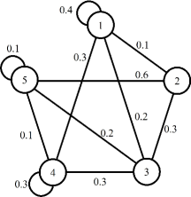
Figure 1: Topology structure of the undirected graph

First, let $C\!=\!0.2$, step-sizes $\hat{\alpha}\!=\!\frac{0.35(\ln(2000))^{2}}{2000}\approx 10^{-2},\hat{\beta}\!=\!\frac{0.3}{2000^{0.75}}\approx 10^{-3}$, the sample-size $\hat{\gamma}\!=\!\lfloor 0.24\cdot 2000^{0.7}\rfloor+1=50$, $\delta_{k}=\frac{1}{(k+1)^{3}}$, the quantizer in the form of (3) with $\Delta=1,5,10$, and the privacy noise parameter $\sigma_{k}=(k+5)^{\sigma}$ with $\sigma=-0.1,0.1,0.2$, respectively. Then, it can be seen that Assumptions 2-4 hold. The training and testing accuracy on the “MNIST” dataset are presented in Fig. 2 and 3, from which one can see that as iterations increase, the training and testing accuracy increase. More importantly, the smaller $\Delta$ and $\sigma$ are, the better the accuracy Algorithm 1 achieves. This is consistent with (33) in Theorem 2, since the smaller $\Delta$ and $\sigma$ are, the smaller the quantization error and the noise variances are, and the faster Algorithm 1 converges.

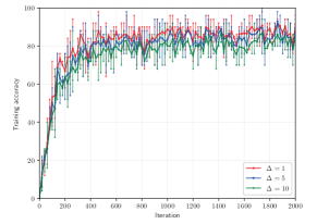
(a) Training accuracy

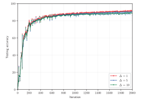
(b) Testing accuracy

Figure 2: Accuracy of Algorithm 1 with $\Delta=1,5,10$

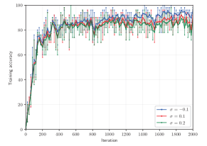
(a) Training accuracy

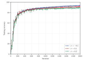
(b) Testing accuracy

Figure 3: Accuracy of Algorithm 1 with $\sigma=-0.1,0.1,0.2$

Next, we set $\Delta=1,\sigma=0.1$ in Algorithm 1. Then, the comparison of accuracy between Algorithm 1 and the methods of [24, 25, 26, 27, 29, 30, 28] is presented in Fig. 4LABEL:sub@fig4a and 4LABEL:sub@fig4b, respectively. To ensure a fair comparison, we set the same step-sizes in [24, 26, 30] as this paper, and the step-sizes in [25, 27, 29, 28] as chosen therein. In addition, we set sample-sizes in [24, 25, 26, 27, 29, 30, 28] as chosen therein. From Fig. 4LABEL:sub@fig4a and 4LABEL:sub@fig4b, it can be seen that Algorithm 1 achieves better accuracy than [24, 25, 26, 27, 29, 30, 28].

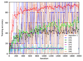
(a) Training accuracy

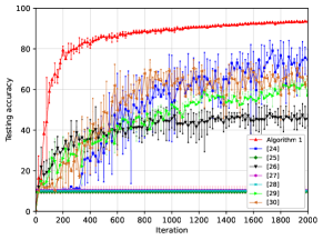
(b) Testing accuracy

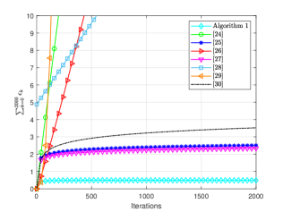
(c) $\sum_{k=0}^{2000}\epsilon_{k}$ under same $\sigma_{k},\delta_{k}$

Figure 4: Comparison of accuracy and differential privacy

Meanwhile, under the same privacy noise parameter $\sigma_{k}$ and differential privacy parameter $\delta_{k}$, the comparison of the cumulative differential privacy budget $\sum_{k=0}^{2000}\epsilon_{k}$ is presented in Fig. 4LABEL:sub@fig4c, which implies that the cumulative differential privacy budget of Algorithm 1 is bounded by finite constants over infinite iterations, while the cumulative differential privacy budget in [24, 25, 26, 27, 29, 30, 28] goes to infinity over infinite iterations. Based on the above discussions, Algorithm 1 not only converges, but also provides a smaller cumulative differential privacy budget over infinite iterations.

Finally, the relationship of the cumulative differential privacy budget $\epsilon$ over infinite iterations, the privacy noise parameter $\sigma$ and sample-size parameter $\gamma$ is presented in Fig. 5, from which one can see that as the privacy noise parameter $\sigma$ and the sample-size parameter $\gamma$ increase, the cumulative differential privacy budget $\epsilon$ decrease. This is consistent with the privacy analysis in Subsection 3.2. Moreover, in the first 2000 iterations, the cumulative differential privacy budget $\sum_{k=0}^{2000}\epsilon_{k}=0.4861$ and $\sum_{k=0}^{2000}\delta_{k}=0.2021$, which is consistent with Theorem 1.

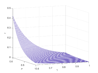
Figure 5: Relationship of $\epsilon$, $\sigma$ and $\gamma$

5 Conclusion

In this paper, we have presented a differentially private distributed nonconvex stochastic optimization algorithm with quantized communications. In the proposed algorithm, increasing privacy noises are added to each node’s local states to prevent information leakage, and then a probabilistic quantizer is employed on noise-perturbed states to improve communication efficiency. By employing the subsampling method controlled through the sample-size parameter, the differential privacy level of the proposed algorithm is enhanced compared with the existing ones. Under the Polyak-Łojasiewicz condition, the mean and high-probability convergence rate and the oracle complexity of the proposed algorithm are given. Meanwhile, the trade-off between the cumulative differential privacy budget and the mean convergence rate is shown. Finally, a numerical example of the distributed training of CNN on the “MNIST” dataset is given to verify the effectiveness of the proposed algorithm.

References

- [1] M. Zhu and S. Martínez, “On distributed convex optimization under inequality and equality constraints,” IEEE Trans. Autom. Control, vol. 57, no. 1, pp. 151–164, 2011.
- [2] M. Zhu and S. Martínez, “An approximate dual subgradient algorithm for multi-agent non-convex optimization,” IEEE Trans. Autom. Control, vol. 58, no. 6, pp. 1534–1539, 2013.
- [3] T. T. Doan, S. T. Maguluri, and J. Romberg, “Fast convergence rates of distributed subgradient methods with adaptive quantization,” IEEE Trans. Autom. Control, vol. 66, no. 5, pp. 2191–2205, 2021.
- [4] T. T. Doan, S. T. Maguluri, and J. Romberg, “Convergence rates of distributed gradient methods under random quantization: a stochastic approximation approach,” IEEE Trans. Autom. Control, vol. 66, no. 10, pp. 4469–4484, 2021.
- [5] R. Xin, U. A. Khan, and S. Kar, “A fast randomized incremental gradient method for decentralized nonconvex optimization,” IEEE Trans. Autom. Control, vol. 67, no. 10, pp. 5150–5165, 2022.
- [6] Z. Jiang, A. Balu, C. Hegde, and S. Sarkar, “Collaborative deep learning in fixed topology networks,” in Proc. Adv. Neural Inf. Process. Syst., Long Beach, CA, USA, 2017, vol. 30, pp. 5904–5914.
- [7] K. Lu, H. Wang, H. Zhang, and L. Wang, “Convergence in high probability of distributed stochastic gradient descent algorithms,” IEEE Trans. Autom. Control, doi: 10.1109/TAC.2023.3327319, 2024.
- [8] A. Reisizadeh, H. Taheri, A. Mokhtari, H. Hassani, and R. Pedarsani, “Robust and communication-efficient collaborative learning,” in Proc. Adv. Neural Inf. Process. Syst., Vancouver, BC, Canada, 2019, vol. 32, pp. 8388–8399.
- [9] Z. Zhang, Y. Zhang, D. Guo, S. Zhao, and X. Zhu, “Communication-efficient federated continual learning for distributed learning system with non-iid data,” Sci. China Inf. Sci., vol. 66, no. 2, 2023, Art. no. 122102.
- [10] K. Ge, Y. Zhang, Y. Fu, Z. Lai, X. Deng, and D. Li, “Accelerate distributed deep learning with cluster-aware sketch quantization,” Sci. China Inf. Sci., vol. 66, no. 6, 2023, Art. no. 162102.
- [11] J. Lei, P. Yi, J. Chen, and Y. Hong, “Distributed variable sample-size stochastic optimization with fixed step-sizes,” IEEE Trans. Autom. Control, vol. 67, no. 10, pp. 5630–5637, 2022.
- [12] J. F. Zhang, J. W. Tan, and J. Wang, “Privacy security in control systems,” Sci. China Inf. Sci., vol. 64, no. 7, 2021, Art. no. 176201.
- [13] Y. Lu and M. Zhu, “Privacy preserving distributed optimization using homomorphic encryption,” Automatica, vol. 96, pp. 314–325, 2018.
- [14] Y. L. Mo and R. M. Murray, “Privacy preserving average consensus,” IEEE Trans. Autom. Control, vol. 62, no. 2, pp. 753–765, 2017.
- [15] Y. Lou, L. Yu, S. Wang, and P. Yi, “Privacy preservation in distributed subgradient optimization algorithms,” IEEE Trans. Cybern., vol. 48, no. 7, pp. 2154–2165, 2018.
- [16] Y. Wang, “Privacy-preserving average consensus via state decomposition,” IEEE Trans. Autom. Control, vol. 64, no. 11, pp. 4711–4716, 2019.
- [17] Y. Lu and M. Zhu, “On privacy preserving data release of linear dynamic networks,” Automatica, vol. 115, 2020, Art. no. 108839.
- [18] J. Le Ny and G. J. Pappas, “Differentially private filtering,” IEEE Trans. Autom. Control, vol. 59, no. 2, pp. 341–354, 2014.
- [19] C. Dwork and A. Roth, “The algorithmic foundations of differential privacy,” Found. Trends Theor. Comput. Sci., vol. 9, nos. 3–4, pp. 211–407, 2014.
- [20] X. K. Liu, J. F. Zhang, and J. Wang, “Differentially private consensus algorithm for continuous-time heterogeneous multi-agent systems,” Automatica, vol. 122, 2020, Art. no. 109283.
- [21] J. Wang, J. F. Zhang, and X. He, “Differentially private distributed algorithms for stochastic aggregative games,” Automatica, vol. 142, 2022, Art. no. 110440.
- [22] X. Chen, C. Wang, Q. Yang, T. Hu, and C. Jiang, “Locally differentially private high-dimensional data synthesis,” Sci. China Inf. Sci., vol. 66, no. 1, 2023, Art. no. 112101.
- [23] J. Wang, J. Ke, and J. F. Zhang, “Differentially private bipartite consensus over signed networks with time-varying noises,” IEEE Trans. Autom. Control, doi: 10.1109/TAC.2024.3351869, 2024.
- [24] C. Li, P. Zhou, L. Xiong, Q. Wang, and T. Wang, “Differentially private distributed online learning,” IEEE Trans. Knowl. Data Eng., vol. 30, no. 8, pp. 1440–1453, 2018.
- [25] Z. Huang, R. Hu, Y. Guo, E. Chan-Tin, and Y. Gong, “DP-ADMM: ADMM-based distributed learning with differential privacy,” IEEE Trans. Inf. Forensics Secur., vol. 15, pp. 1002–1012, 2020.
- [26] J. Ding, G. Liang, J. Bi, and M. Pan, “Differentially private and communication efficient collaborative learning,“ in Proc. AAAI Conf. Artif. Intell., Palo Alto, CA, USA, 2021, vol. 35, no. 8, pp. 7219–7227.
- [27] C. Gratton, N. K. D. Venkategowda, R. Arablouei, and S. Werner, “Privacy-preserved distributed learning with zeroth-order optimization,” IEEE Trans. Inf. Forensics Secur., vol. 17, pp. 265–279, 2022.
- [28] C. Liu, K. H. Johansson, and Y. Shi, “Distributed empirical risk minimization with differential privacy,” Automatica, vol. 162, 2024, Art. no. 111514.
- [29] J. Xu, W. Zhang, and F. Wang, “A (DP) 2 SGD: asynchronous decentralized parallel stochastic gradient descent with differential privacy,” IEEE Trans. Pattern Anal. Mach. Intell., vol. 44, no. 11, pp. 8036–8047, 2022.
- [30] Y. Wang and T. Başar, “Decentralized nonconvex optimization with guaranteed privacy and accuracy,” Automatica, vol. 150, 2023, Art. no. 110858.
- [31] Y. Wang and T. Başar, “Quantization enabled privacy protection in decentralized stochastic optimization,” IEEE Trans. Autom. Control, vol. 68, no. 7, pp. 4038–4052, 2023.
- [32] G. Yan, T. Li, K. Wu, and L. Song, “Killing two birds with one stone: quantization achieves privacy in distributed learning,” Digit. Signal Process., vol. 146, 2024, Art. no. 104353.
- [33] A. Xie, X. Yi, X. Wang, M. Cao, and X. Ren, “Compressed differentially private distributed optimization with linear convergence,” IFAC-PapersOnLine, vol. 56, no. 2, pp. 8369–8374, 2023.
- [34] H. Karimi, J. Nutini, and M. Schmidt, “Linear convergence of gradient and proximal-gradient methods under the polyak-łojasiewicz condition,” in Proc. Mach. Learn. Knowl. Discov. Databases Euro. Conf., Riva del Garda, Italy, 2016, pp. 795–811.
- [35] T. C. Aysal, M. J. Coates, and M. G. Rabbat, “Distributed average consensus with dithered quantization,” IEEE Trans. Signal Process., vol. 56, no. 10, pp. 4905–4918, 2008.
- [36] L. Zhu, Z. Liu, and S. Han, “Deep leakage from gradients,” in Proc. Adv. Neural Inf. Process. Syst., Vancouver, BC, Canada, 2019, vol. 32, pp. 14774–14784.
- [37] S. Bubeck, “Convex optimization: algorithms and complexity,” Found. Trends Theor. Comput. Sci., vol. 8, nos. 3-4, pp. 231–357, 2015.
- [38] V. A. Zorich, “Integration,” in Mathematical analysis I, Berlin, German: Springer-Verlag, 2015, ch. 6, sec. 2, pp. 349–360.
- [39] R. A. Horn and C. R. Johnson, “Hermitian matrices, symmetric matrices, and congruences,” in Matrix analysis, Cambridge, U.K.: Cambridge University Press, 2012, ch. 4, sec. 2, pp. 234–239.
- [40] Y. S. Chow and H. Teicher, “Integration in a probability space,”in Probability theory: independence, interchangeability, martingales, New York, NY, USA: Springer-Verlag, 2012, ch. 4, sec. 1, pp. 84–92.
- [41] Y. LeCun, C. Cortes, and C. J. C. Burges, 1998, “The MNIST database of handwritten digits,” National Institute of Standards and Technology. [Online]. Available: http://yann.lecun.com/exdb/mnist/