Mathematical Foundation and Corrections for Full-Range Head Pose Estimation

Abstract

Numerous works concerning head pose estimation (HPE) offer algorithms or proposed neural network-based approaches for extracting Euler angles from either facial key points or directly from images of the head region. However, many works failed to provide clear definitions of the coordinate systems and Euler or Tait–Bryan angles orders in use. It is a well-known fact that rotation matrices depend on coordinate systems, and yaw, roll, and pitch angles are sensitive to their application order. Without precise definitions, it becomes challenging to validate the correctness of the output head pose and drawing routines employed in prior works. In this paper, we thoroughly examined the Euler angles defined in the 300W-LP dataset, head pose estimation such as 3DDFA_v2, 6D-RepNet, WHENet, etc, and the validity of their drawing routines of the Euler angles. When necessary, we infer their coordinate system and sequence of yaw, roll, pitch from provided code. This paper presents (1) code and algorithms for inferring coordinate system from provided source code, code for Euler angle application order and extracting precise rotation matrices and the Euler angles, (2) code and algorithms for converting poses from one rotation system to another, (3) novel formulae for 2D augmentations of the rotation matrices, and (4) derivations and code for the correct drawing routines for rotation matrices and poses. This paper also addresses the feasibility of defining rotations with Wikipedia & SciPy’s right-handed coordinate system, which makes the Euler angle extraction much easier for full-range head pose research. Our code will be released in https://github.com/foresee-ai/hpe_math.

Keywords Rotation Matrix  $\cdot$ Euler Angles  $\cdot$ Full-range Angles $\cdot$ Head Pose Estimation  $\cdot$ Facial Land Marks  $\cdot$ Face Analysis  $\cdot$ Facial Key-point Detection  $\cdot$ 300W_LP  $\cdot$ CMU Panoptic Dataset  $\cdot$ AGORA

1 Introduction

Head Orientation Estimation has evolved significantly, driven by the increasing integration of computer vision and vision-based deep learning. Early approaches often relied on facial key-point detection and images with fixed rotation angle labeling. However, this field has witnessed a paradigm shift with the advent of deep learning, especially convolutional neural networks (CNNs). The ability of deep learning models to automatically learn hierarchical features from data has significantly improved the accuracy and robustness of head orientation estimation algorithms.

Nevertheless, it is noteworthy that many current works on head pose estimation lack fundamental definitions of the coordinate systems employed. Additionally, some methodologies borrowed facial landmark-based code intended for limited (mostly camera-facing) head pose estimation and applied to a broader range of head poses. Moreover, facial orientation drawing routines are often borrowed from code designed for a different coordinate system. This deficit in mathematical clarity also deters the application of standard geometric 2D image augmentations, such as flipping and rotation. This paper aims to address these gaps in understanding.

The structure of this paper is as follows: we start by presenting classical Head Pose Estimation (HPE) approaches and formulate the foundational mathematical concepts involved. Subsequently, we conduct a comprehensive analysis of select datasets, employing symbolic computation techniques where necessary, to infer key parameters, particularly when clear definitions of coordinate systems and Euler angles are absent throughout the literature. We also delve into the conversion of Euler angles between different coordinate systems, providing code implementations where relevant. Furthermore, we identify and highlight inaccuracies or imprecision in both code and literature of some previous works.

Lastly, we present a comprehensive derivation of the transformation of rotation matrices under typical 2D image augmentations. These derivations enable improved model performance without the necessity of increasing the volume of training images. To our knowledge, these derivations have not been utilized or documented in current literature related to Head Pose Estimation (HPE).

2 Related Work

This paper will focus on monocular RGB images. Classical approaches, such as template matching and detector arrays, related to head pose estimation (HPE) preceding 2008 can be found in the survey paper [1]. Deformable models are thoroughly discussed in [2], [3], [4], and [5] and were used to create the commonly used synthetic pose dataset such as 300W_LP [3].

2.1 Head pose estimation

Head pose estimation can be divided into two categories, with and without facial landmarks. Traditionally, head orientation only makes sense when facial features are visible. See Fig. 1 for reference. Obviously, when people are facing away from the camera, no key points can be detected, and this method will not work. Dlib[6] is one of the pioneers in using face landmarks for prediction.

From facial landmarks, we can mathematically derive the 3D transformations involved in changing the 2D projected shape of facial landmarks with the help of a "standard" face. Later, with the advent of deep learning, researchers start to explore the possibility of utilizing convolutional neural networks to predict the three Euler angles directly, for example, Hopenet[7] and WHENet[8]. However, the Euler-angle loss easily leads to discontinuity because every angle has multiple numerical representations, e.g., $0\degree=360\degree$. To avoid such discontinuity, 6D-RepNet [9] (including 6D-RepNet360[10]) and TriNet[11] predict the $3\times 2$ and $3\times 3$ rotation matrices respectively. 6D-RepNet still applies the Euler-angle evaluation metric for comparison with other HPE methods. However, due to the natural scarcity of the labeled data, most of these approaches still utilize datasets created/ synthesized from facial key-points approaches. Next, we will review some of the mathematical basics involved in HPE.

Figure 1: Dlib’s 68 facial landmarks. [12]

2.2 Head pose dataset creation

The 300W across Large Poses (300W-LP) dataset [3] was based on 300W [13], which standardized multiple alignment datasets with 68 landmarks, including AFW [14], LFPW [15], HELEN [16], IBUG [13], and XM2VTS [17]. 300W_LP’s labeled Euler angles are extracted from the rotation matrix estimated from [3]’s 3D Dense Face Alignment (3DDFA), which applies Blanz et al.’s morphable model 3DMM [2], to obtain the standard and rotated 3D faces tailored for an image. While the labeled poses of 300W_LP have been widely used for head pose training or testing, we found multiple 300W_LP’s Euler-angle formulas/implementations are used for papers on HPE and 3D dense face alignment [[3], [18], [4], [9], [10]]. This motivated us to find out which formulas align to 300W_LP’s rotation and pose definitions.

While 300W_LP offered pose labels limited to frontal views, the CMU Panoptic Dataset [19] provided extensive 3D facial landmarks for multiple individuals captured from cameras spanning an entire hemisphere, which can be turned into head pose. WHENet [8] pioneered techniques to transform the CMU Panoptic Dataset into a comprehensive head pose estimation (HPE) dataset covering a larger range of angles. 6D-RepNet360 [10] used WHENet’s CMU Panoptic pose data generation method/code to improve its previous range limited 6D-RepNet [9].

3 Rotations and the Euler angles

Definition 3.1.

A 3D rotation matrix in a 3D Cartesian coordinate system is a transformation matrix $R\in SO(3)$, where $SO(3)$ is the group of invertible 3 $\times$ 3 matrices such that $det(R)=1$ and $R\times R^{T}=R^{T}\times R=I_{3}$. Each column of R represents each rotated axis so that R can be used to rotate objects. Then for every (row) vector $\bm{v}\in\mathbb{R}^{3}$, We assume the application of the rotation is to the left of the vector, i.e. the rotated vector $\bm{v}_{rotated}$ is defined as follows: $\bm{v}_{rotated}=(R\times\bm{v}^{T})^{T}$.

Definition 3.2.

Here, we assume the existence of two coordinate systems, one with the origin at the center of the head and moving/rotating along with the head, is called intrinsic coordinate system. The other, without loss of generality, coincides with the intrinsic coordinate system initially but does not move along with the head and is called extrinsic coordinate system. The 3D rotation R, defined by Definition 3.1, can also be refined by 2 conventions, extrinsic and intrinsic rotations. Intrinsic rotations [20] are elemental rotations that occur about the axes of the intrinsic coordinate system, which axes are denoted in uppercase XYZ. Extrinsic rotations [20] are elemental rotations that occur about the axes of the extrinsic coordinate system whose axes are denoted in lowercase, say $xyz$. The intrinsic XYZ-coordinate system remains fixed from the perspective of a targeted human head. In contrast, the extrinsic xyz-coordinate system remains fixed from the perspective of external observers.

It’s also possible to parameterize the rotation matrix with a smaller set of numbers[21]. One of the most common sets of parameters is the Euler angles defined by Leonhard Euler[22]. The Euler angles are the three elemental angles yaw, pitch, and roll representing the orientation of a rigid body to a fixed coordinate system. We use handedness(the right-handed or left-handed rule) along each axis to define the positive direction of each Euler angle. Please note that this is different from using handedness to define left- or right-handed coordinate systems as in some other conventions. Although they are associated with the three coordinate axes, users must define the desired order to recover the rotation matrices uniquely.

To avoid ambiguity, we define $\bm{yaw=0,pitch=0},$ and $\bm{roll=0}$ to represent the straight frontal face as shown on the left in Fig. 5 and restrict $\bm{(-\pi,\pi]}$ to be the range of yaw, roll, and pitch. The range of yaw, roll, and pitch is especially important for the loss functions for deep learning based approaches based on the Euler angles. For example, 300W_LP adapts our definition and its ranges of pitch, yaw, and roll are $(-167\degree,107\degree),[-90\degree,90\degree],$ and $(-159\degree,94\degree)$ respectively.

To find the Euler angles of a rotation, E. Bernardes’s Quaternion to Euler angles conversion [23] describes the mathematical form of decomposing the 3D rotation matrix into the product of three elemental (axis-wise) rotations:

$$R=R_{\bm{e_{3}}}(\theta_{3})\times R_{\bm{e_{2}}}(\theta_{2})\times R_{\bm{e_{1}}}(\theta_{1})$$ (1)

where $R_{\bm{e_{i}}}(\theta)$ represents a rotation by the angle $\theta$ around the unit axis vector $\bm{e_{i}}$. These consecutive axes must be orthogonal, i.e., $\bm{e_{1}}\cdot\bm{e_{2}}=\bm{e_{2}}\cdot\bm{e_{3}}=0$. In addition, $\bm{e_{1}}$, $\bm{e_{2}}$ and $\bm{e_{3}}$ are orthogonal unit vectors and $\bm{e_{3}}=\epsilon\cdot(\bm{e_{1}}\times\bm{e_{2}})$ in which $\epsilon=(\bm{e_{1}}\times\bm{e_{2}})\cdot\bm{e_{3}}=\pm 1$.

The following Lemma demonstrates the difference between the two rotation types.

Lemma 3.3.

Suppose $\bm{e_{1}}$ and $\bm{e_{2}}$ are the orthogonal unit axis vectors defined in Definition 3.2. Given the elemental rotation sequence, first rotating $\theta_{1}$ along $\bm{e_{1}}$, then rotating $\theta_{2}$ along $\bm{e_{2}}$, we can derive that the intrinsic rotation is $\Lambda=R_{\bm{e_{1}}}(\theta_{1})\times R_{\bm{e_{2}}}(\theta_{2})$, and the extrinsic rotation is $\Sigma=R_{\bm{e_{2}}}(\theta_{2})\times R_{\bm{e_{1}}}(\theta_{1})$.

Proof.

Note that the extrinsic coordinate system stays the same under rotations and also for angle $\phi$ and axis $\bm{e}$, $R^{-1}_{\bm{e}}(\phi)=R^{t}_{\bm{e}}(\phi)=R_{\bm{e}}(-\phi)$. Observe the extrinsic rotation matrix is just successively applying rotation matrices and trivially $\Sigma=R_{\bm{e_{2}}}(\theta_{2})\times R_{\bm{e_{1}}}(\theta_{1})$. The intrinsic rotation, denoted by $\Lambda$, can be defined by $\bm{v_{rotated}}^{T}=\Lambda\times\bm{v}^{T}$, where both $\bm{v_{rotated}}$ and $\bm{v}$ are row vectors with the coordinates in the extrinsic $xyz$-coordinate system. Note from the perspective of the human head, rotating $\phi$ about an axis $\bm{e}$ in the intrinsic coordinate system is equivalent to rotating $-\phi$ extrinsically with intrinsic coordinate system unchanged, so we have $\bm{v}^{T}=R_{\bm{e_{2}}}(-\theta_{2})\times R_{\bm{e_{1}}}(-\theta_{1})\times\bm{v_{rotated}}^{T}$, $\implies$ $\bm{v}^{T}=R^{-1}_{\bm{e_{2}}}(\theta_{2})\times R^{-1}_{\bm{e_{1}}}(\theta_{1})\times\bm{v_{rotated}}^{T}$ (especially for $\theta_{1}=\theta_{2}=90\degree$, $\bm{v}^{T}=R^{-1}_{X}(90\degree)\times R^{-1}_{Y}(90\degree)\times\bm{v_{rotated}}^{T}$ as demonstrated in the following figure 2). Then $\Lambda^{-1}=R^{-1}_{\bm{e_{2}}}(\theta_{2})\times R^{-1}_{\bm{e_{1}}}(\theta_{1})=(R_{\bm{e_{1}}}(\theta_{1})\times R_{\bm{e_{2}}}(\theta_{2}))^{-1}$. So we get $\Lambda=R_{\bm{e_{1}}}(\theta_{1})\times R_{\bm{e_{2}}}(\theta_{2})$. ∎

Figure 2: Demonstration of successive application of rotations in the case of $\theta_{1}=\theta_{2}=90\degree$

Theorem 3.4.

Suppose $\bm{e_{1}}$, $\bm{e_{2}}$, and $\bm{e_{3}}$ are the three orthogonal unit axis vectors defined in Definition 3.2. Given the elemental rotation sequence, first rotating $\theta_{1}$ along $\bm{e_{1}}$, then rotating $\theta_{2}$ along $\bm{e_{2}}$, last rotating $\theta_{3}$ along $\bm{e_{3}}$, the intrinsic and extrinsic rotations, denoted by $R_{intrinisc}$ and $R_{extrinisc}$ respectively, can be expressed as follows:

$$\begin{split}R_{intrinsic}&=R_{\bm{e_{1}}}(\theta_{1})\times R_{\bm{e_{2}}}(\theta_{2})\times R_{\bm{e_{3}}}(\theta_{3})\\ R_{extrinsic}&=R_{\bm{e_{3}}}(\theta_{3})\times R_{\bm{e_{2}}}(\theta_{2})\times R_{\bm{e_{1}}}(\theta_{1})\end{split}$$ (2)

Proof.

Apply Lemma 3.3 twice and prove the equality 2 holds. ∎

Based on Theorem 3.4 and the fact that matrix multiplications are non-commutative, we can conclude (1) the intrinsic and extrinsic rotation matrices are usually different; and (2) the axis-sequence (the rotating sequence of the three axes) matters for identifying the multiplicative order of the elemental rotation matrices to compute the real rotation matrix $R$. For example, the intrinsic XYZ-sequence rotation yields $R_{X}\times R_{Y}\times R_{Z}$ while the intrinsic ZYX-sequence rotation yields $R_{Z}\times R_{Y}\times R_{X}$.

One important observation from Lemma 3.3 is every sequence of intrinsic rotations has an equivalent sequence of extrinsic rotations in exact reverse order.

To summarize, we suggest HPE paper authors or dataset creators give well-defined rotation system for HPE which should composed of the following: (1) Specify the 3D Cartesian coordinate system used, (2) Each axis’s handedness and associated Euler angle (if applicable), (3) Range of yaw, pitch, and roll (if applicable), and (4) The yaw, pitch, and roll rotation sequence (if applicable). For simplicity, we also refer a coordinate (or rotation) system A adapting B’s system to A’s system follows B’s system disregarding transitions and scaling.

4 Wikipedia’s intrinsic ZYX-sequence Rotations

The intrinsic rotation system employed by Wikipedia deserves attention for its widespread adoption among engineers and incorporation into SciPy’s implementation for rotations and Euler angles.

Definition 4.1.

Wikipedia’s intrinsic ZYX-sequence Rotations are defined in Wikipedia’s right-handed coordinate system [20], and follows the intrinsic ZYX-sequence, which has the order that first applies $R_{Z}$, then $R_{Y}$, last $R_{X}$. Within Wikipedia’s system, yaw, pitch, and roll are defined as the rotations along the Z-, Y-, and X-axes by the angles yaw, pitch, and roll. We have the elemental rotations and rotation matrix, denoted by $R_{S}$, as follows:

$$\begin{split}R_{X}(p)&=\begin{bmatrix}1&0&0\\ 0&cos(p)&-sin(p)\\ 0&sin(p)&cos(p)\end{bmatrix},R_{Y}(y)=\begin{bmatrix}cos(y)&0&sin(y)\\ 0&1&0\\ -sin(y)&0&cos(y)\end{bmatrix},R_{Z}(r)=\begin{bmatrix}cos(r)&-sin(r)&0\\ sin(r)&cos(r)&0\\ 0&0&1\end{bmatrix}\\ \\ R_{S}&=R_{Z}(y)\times R_{Y}(p)\times R_{X}(r)\\ &=\begin{bmatrix}cos(y)cos(p)&cos(y)sin(p)sin(r)-sin(y)cos(r)&cos(y)sin(p)cos(r)+sin(y)sin(r)\\ sin(y)cos(p)&sin(y)sin(p)sin(r)+cos(y)cos(r)&sin(y)sin(p)cos(r)-cos(y)sin(r)\\ -sin(p)&cos(p)sin(r)&cos(p)cos(r)\end{bmatrix}.\end{split}$$ (3)

$y,p,r$ in Formula 3 are the Euler angles, yaw, pitch, and roll, respectively.

Figure 3: SciPy and Wikipedia’s coordinate system with right-handed

According to SciPy Rotation class documentation, [24], its Euler-angle implementation follows Wikipedia’s right-handed coordinate system. The convenient script (shown in Listing 20) allows us to quickly compute the Euler angles (pitch, yaw, and roll) without really dealing with the hassle.

We re-emphasize here that Wikipedia and SciPy share the same rotation system, i.e., right-handed intrinsic ZYX-sequence rotations as demonstrated in Fig. 3.

4.1 Three-line drawing & Euler-angle closed-form solution in Wikipedia/SciPy’s right-handed coordinate system

Three-line drawings are generally utilized in HPE papers to visually represent head poses in 2D images. A popular convention is nose direction in blue, neck direction in green, and left face direction in red, as illustrated in Figure 9. Under Wikipedia’s coordinate system, for simplicity, we ignore camera intrinsic and regard the three-line drawing as a projection of the coordinate axes $X,Y,-Z$ to the 2D $ZY$ plane, with $X$-axis in blue, $Y$-axis in red and $-Z$-axis in green.

More precisely, before projecting onto the image’s 2D Cartesian coordinate system, we first apply a coordinate transformation to the rotation matrix in SciPy’s coordinate system into the one with the Z-axis pointing downwards. Then, project the transformed matrix onto the YZ-plane to get the vectors associated with the three RGB lines. As in 4, the new rotation matrix, $R^{\textbf{draw}}_{S}$, represents the rotation $R_{S}(y,p,r)$ (defined by Formula 3) under SciPy’s coordinate system) in the new 3D coordinate system with Z-axis pointing downward. Finally, apply the YZ-plane projection.

$$\begin{split}R^{\bm{draw}}_{S}=T_{S}\times&R_{S}(y,p,r)\times T^{-1}_{S},\quad where\quad T_{S}=\begin{bmatrix}1&0&0\\ 0&1&0\\ 0&0&-1\end{bmatrix}.\\ and\quad Proj_{YZ}&=\begin{bmatrix}0&1&0\\ 0&0&1\end{bmatrix}\times\quad R^{\bm{draw}}_{S}.\end{split}$$ (4)

The above formula, Formula 4, also reveals one important observation: the key of this drawing (matrix) solely depends on the rotation matrix itself. Therefore the Euler angles are not necessary for the drawing if the rotation matrix is provided, even if yaw, roll, and pitch are provided they still need to be turned into the associated rotation matrix before the actual drawing.

Slabaugh, G. G’s [25] provides the Euler angle extraction pseudo code for Wikipedia’s rotation, and its extracted Euler angles lie within $[0,2\pi]$. To help visualize the head poses, we prefer the range $(-\pi,\pi]$. So, we modified Slabaugh’s pseudo code to suit our needs. The two pitch-yaw-roll closed-form conversions from a rotation matrix’s Python code implementation are shown in Listing (21).

Experiments show that the difference between our method (Listing 21) and SciPy’s is minuscule, which is caused by the nature of machine epsilon. SciPy’s and our implementations maintain excellent numerical stability; the Frobenius norms of these yaw-roll-pitch solutions only differ from the ground-truth poses roughly within 2 $\times$ machine epsilon. See Fig. 13 for the comparison.

5 The 300W-LP dataset

Like 300W dataset [26], 300W-LP adopts the proposed face profiling to generate 61,225 samples across large poses (1,786 from IBUG, 5,207 from AFW [14], 16,556 from LFPW [15], and 37,676 from HELEN [16], XM2VTS [17] is not used), which is further expanded to 122,450 samples with flipping. The literature itself lacks the basic definition of coordinate and rotation system as mentioned in Section 3.1, we will try to infer them from the provided code implementations in the following sections.

5.1 Derivation of 300W-LP’s rotation system based on its implementation [27]

While the original code adopts the Base Face Model with neck, its successor [3] uses the BFM without the ear/neck region. Because both BMFs use the same coordinate system, we decided to use the latter as our Base Face Model (as [27] provided BFM link is no longer valid) to derive 300W_LP’s rotation system. First, we can identify the coordinate system used in 300W-LP from the BMF without the neck. Then, the original code provides the elemental rotation matrices for the Euler angles and the axes-sequence (see Formula 5). Combining the coordinate system, elemental rotations, and intrinsic XYZ-sequence (i.e., pitch-yaw-roll order), we conclude that 300W_LP’s Euler angles adapt the left-handed rotation. Fig. 4 demonstrates our inferred definitions for the coordinate system and Euler angle used in 300W-LP’s annotations, as shown below. Note $R^{left}_{X}(p)$ means rotation about $X$-axis in left-handed fashion.

$$R^{left}_{X}(p)=\begin{bmatrix}1&0&0\\ 0&cos(p)&sin(p)\\ 0&-sin(p)&cos(p)\end{bmatrix},R^{left}_{Y}(y)=\begin{bmatrix}cos(y)&0&-sin(y)\\ 0&1&0\\ sin(y)&0&cos(y)\end{bmatrix},R^{left}_{Z}(r)=\begin{bmatrix}cos(r)&sin(r)&0\\ -sin(r)&cos(r)&0\\ 0&0&1\end{bmatrix}$$

$$\begin{split}R_{W}(y,p,r)&=R^{left}_{X}(p)\times R^{left}_{Y}(y)\times R^{left}_{Z}(r)\\ &=\begin{bmatrix}cos(y)cos(r)&cos(y)sin(r)&-sin(y)\\ -cos(p)sin(r)+sin(p)sin(y)cos(r)&cos(p)cos(r)+sin(p)sin(y)sin(r)&sin(p)cos(y)\\ sin(p)sin(r)+cos(p)sin(y)cos(r)&-sin(p)cos(r)+cos(p)sin(y)sin(r)&cos(p)cos(y)\end{bmatrix}\end{split}$$ (5)

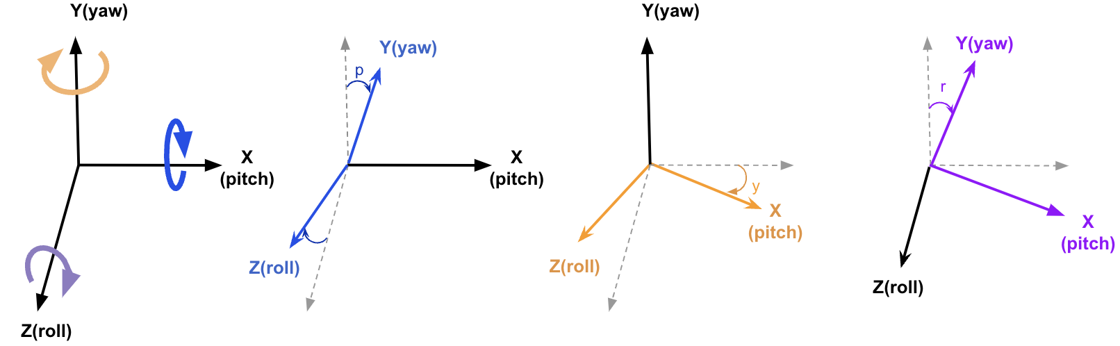
Figure 4: 300W-LP’s elemental rotations

However, we found that Fig. 3 on the right (of our Fig. 5 in below) cited from the original 300W-LP paper [3] demonstrates the right-handed Euler angles instead. To avoid further confusion, from now on, we stick to the left-handed coordinate system shown in Fig, 4 and the left in Fig. 5 as 300W-LP’s Euler angle definition.

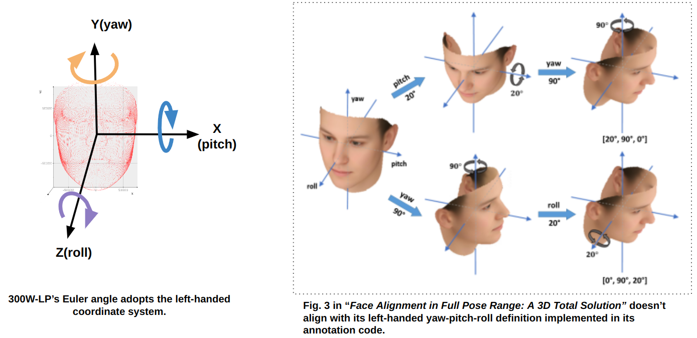
Figure 5: 300W-LP’s Euler angle illustration does not align with what we inferred from its source code

5.2 300W-LP’s 3D face reconstruction

The basic idea for obtaining the rotation matrix from an image is to fit the BFM to the human head in the image and then compute the transformation needed to go from the original BFM to the fitted BFM. [3] proposed the 3D Dense Face Alignment (3DDFA) to obtain the rotated 3D face from an image. Algorithm 3DDFA applies the 3D morph-able model (3DMM) from Blanz et al.’s [2] which describes the 3D face with PCA: $S=\bar{S}+A_{id}\alpha_{id}+A_{exp}\alpha_{exp}$, where S is a 3D face, $\bar{S}$ is the mean BFM, $A_{id}$ [28] is the principle axes trained on the 3D face scans with neutral expression and $\alpha_{id}$ is the shape parameter, $A_{exp}$ [29]is the principle axes trained on the offsets between expression scans and neutral scans and $\alpha_{exp}$ is the expression parameter. The 3D face is then projected onto the image plane with a Weak Perspective Projection: $V(p)=f\ast Pr\ast R\ast S+t_{2d}$, where $V(p)$ is the 2D positions of model vertexes, $f$ is the scale factor, $Pr=\begin{bmatrix}1&0&0\\ 0&1&0\end{bmatrix}$ , $R$ is the rotation matrix calculated from the Euler angles, and $t_{2d}$ is the translation vector. Fig. 6 shows the predicted 3D face model through the non-scaling, non-transition, and rotation-only computation.

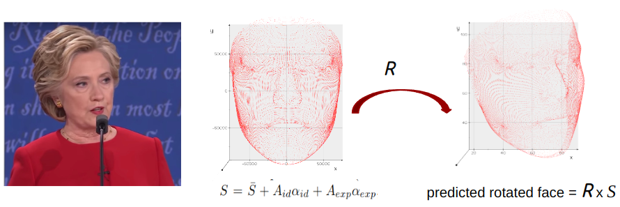
Figure 6: Non-scaled, non-transitional, rotated 3D Face by 3DDFA

The cited paragraph (shown in Fig. 7), from Section 5.1, in [3] explains how its 3DDFA implementation prevents the fitting errors due to a profile face rotated by a small yaw angle or the default closed-mouth parameters for an open-mouth face. To avoid such errors, it defines the ground-truth rotation ${R^{g}}$ to be the one from $S=\bar{S}+A_{id}\alpha_{id}+A_{exp}\alpha_{exp}$ to the face points (FP), instead of the one from the BFM (i.e., $\bar{S}$) to FP. We name this approach the FP-perturbation scheme.

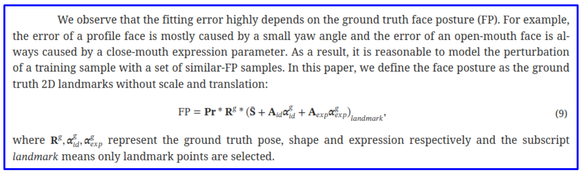
Figure 7: The 3DDFA’s implementation considers FP perturbation

5.3 300W-LP’s drawing method for the Euler angles

Since the code of [3] for 300W_LP dataset didn’t provide any drawing methods about rotation, some of the later works, such as 3DDFA and 3DDFA_v2 adopt the scale orthographic projection, in which it reconstructs the camera extrinsic P, consisting of a non-scaled rotation matrix, i.e., $R_{W}$, and 3D offset, and uses the estimated 3D facial vertices to draw the 3D pose frustums. See Fig. 9. But while the pose-frustum drawing serves the purpose, we find it harder to visualize the nuances among rotations, especially when comparing the ground truth and estimated Euler angles.

In contrast, the three-line drawing, shown in Fig. 9, allows us to visualize the minute differences among the rotations. Here, we follow the convention for drawing, mentioned in section 4.1: the red line stretching toward the left side of the frontal face, the green line stretching from the forehead to the center of the jaw, and the blue line pointing from the nose out. The three lines are perpendicular to each other in the 3-dimensional space, even though sometimes they don’t appear so due to 2D projection.

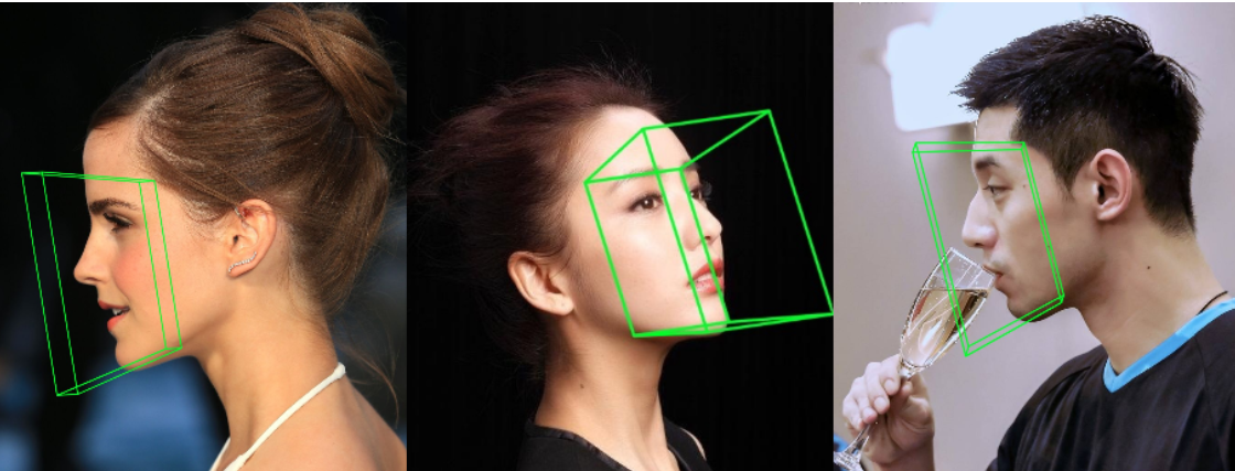
Figure 8: 3DDFA’s Head Pose Drawing, cited from [18]

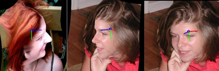
Figure 9: Our Proposed Head Pose Drawing

5.4 Our three-line drawing method for 300W_LP’s pose annotations

We can apply a similar procedure in Section 4.1 by (1) first applying the matrix $T_{W}$ to transform the rotation matrix of 300W_LP’s coordinate system into the one of the Y-axis pointing downwards, and (2) then project the transformed matrix onto the XY-plane of the image’s system. Now, we derive Formula 6 so that the new matrix, $R^{\textbf{draw}}_{W}$, represents the rotation $R_{W}(y,p,r)$ (defined by Formula 5) under 300_LP’s coordinate system) in the 3D coordinate system associated with the image’s system. Then apply the XY-plane projection.

$$R^{\textbf{draw}}_{W}=T_{W}\times R_{W}(y,p,r)\times T^{-1}_{W},\quad where\quad T_{W}=\begin{bmatrix}1&0&0\\ 0&-1&0\\ 0&0&1\end{bmatrix}$$ (6)

The first row of Fig. 11 shows that our proposed three-line drawing routine for 300W_LP’s pose annotations works. Another widely used three-line drawing is the drawing routine draw_axis() (that has been adopted by many papers as shown in Listing 26) which we will carefully compare with our drawing routine in section 6.

5.5 Extracting the Euler angles from a rotation matrix in 300W-LP’s rotation system

Now that we have identified the rotations utilized in 300W-LP following Formula (5), we can proceed to compute the Euler angles from it. We follow Slabaugh, G. G’s [25] Euler angles’ computation except that the range $(-\pi,\pi]$ for the yaw, pitch, and roll values are selected. Although for the pitch and roll, we mainly focus on $[-\pi/2,\pi/2]$ because most head poses occur in this range, including the upside-down human head pose as a result of image augmentations, we cannot eliminate the possibility that true full range may be useful in some occasions. We also use NumPy for trigonometric calculation in code implementations.

For a given rotation $R=(R_{i,j})$ from 300W-LP where $R_{i,j}$ is the $(i,j)$-the entry in R, we can set up the matrix equation (7) to solve for yaw, pitch, and roll.

$$\begin{split}(R_{i,j})&=\begin{bmatrix}cos(y)cos(r)&cos(y)sin(r)&-sin(y)\\ -cos(p)sin(r)+sin(p)sin(y)cos(r)&cos(p)cos(r)+sin(p)sin(y)sin(r)&sin(p)cos(y)\\ sin(p)sin(r)+cos(p)sin(y)cos(r)&-sin(p)cos(r)+cos(p)sin(y)sin(r)&cos(p)cos(y)\end{bmatrix}\end{split}$$ (7)

Equation $R_{0,2}=-\bm{sin}(y)$ gives yaw’s first solution $y_{1}=\bm{arcsin}(-R_{0,2})\in[-\pi/2,\pi/2]$ due to Numpy’s $\bm{arcsin}$ function call. To restrict both yaws in $(-\pi,\pi]$, we derive the second formula of yaw in (8):

$$y_{2}=\begin{cases}\pi-y_{1}&if\verb| |y_{1}\geq 0\\ -\pi-y_{1}&if\verb| |y_{1}<0\end{cases}$$ (8)

Gimbal locks happen when $\bm{cos}(y)=0$, i.e, $y_{1}=y_{2}\text{ and }|y_{i}|=\pi/2$. We will discuss it later.

For the non-Gimbal-lock cases, equivalently $\bm{cos}(y)\neq 0$, we consider the two equations shown in (9).

$$\begin{cases}R_{1,2}&=\bm{sin}(p)\bm{cos}(y)\\ R_{2,2}&=\bm{cos}(p)\bm{cos}(y)\end{cases}$$ (9)

Adapting to Numpy’s $\bm{arctan2}$ makes the solution unique. When applying $\bm{arctan2}$, we must be careful when $\bm{cos}(y)<0$, as mentioned in [25]. It will result in the sign change for both terms, $\bm{sin}(p)$ and $\bm{cos}(p)$, and lead to the wrong angle prediction, $p\pm\pi$, instead of $p$. To avoid such a pitfall, we set pitch $p=\textbf{arctan2}(R_{1,2}/\bm{cos}(y),R_{2,2}/\bm{cos}(y))$, which results in $p$ in $[-\pi,\pi]$. From Numpy’s $\bm{arctan2}$’s document [30], $p$ can be further restricted into the range $(-\pi,\pi)$ due to both numerator and denominator can’t be $\pm\inf$ and $\pm 0$ at the same time. Now, we can formulate pitch as follows:

$$\begin{cases}p_{1}&=\bm{arctan2}(R_{1,2}/\bm{cos}(y_{1}),R_{2,2}/\bm{cos}(y_{1}))\\ p_{2}&=\bm{arctan2}(R_{1,2}/\bm{cos}(y_{2}),R_{2,2}/\bm{cos}(y_{2}))\end{cases}$$ (10)

Formula (8) implies that $\bm{cos}(y_{2})=-\bm{cos}(y_{1})$. Now substitute it back to Formula 10, then we get $\bm{sin}(p_{2})=-\bm{sin}(p_{1})$ and $\bm{cos}(p_{2})=-\bm{cos}(p_{1})$. Hence $p_{1}$ and $p_{2}$ differs by $\pi$. To get both of them inside $(-\pi,\pi]$, we get a simplified formula for pitch, shown in (11):

$$p_{1} =\bm{arctan2}(R_{1,2}/\bm{cos}(y_{1}),R_{2,2}/\bm{cos}(y_{1}))$$ (11)

$$p_{2} =\begin{cases}p_{1}-\pi&\textbf{ if }p_{1}\geq 0\\ p_{1}+\pi&\textbf{ if }p_{1}<0\end{cases}$$ (12)

Similarly, we can derive the formula for roll, as shown in (13):

$$r_{1} =\bm{arctan2}(R_{0,1}/\bm{cos}(y_{1}),R_{0,0}/\bm{cos}(y_{1}))$$ (13)

$$r_{2} =\begin{cases}r_{1}-\pi&\textbf{ if }r_{1}\geq 0\\ r_{1}+\pi&\textbf{ if }r_{1}<0\end{cases}$$ (14)

Gimbal locks occur at $y=\pm\pi/2$. If $y=\pi/2$, $\bm{sin}(y)=1$ and $\bm{cos}(y)=0$ reduce the matrix (7) into (15). In which case, we also find that $R_{1,0}=\bm{sin}(p-r)$ and $R_{1,1}=\bm{cos}(p-r)$. So we have $p-r=\bm{arctan2}(R_{1,0},R_{1,1})$. While there are infinitely many solutions for $p$ and $r$, to prevent $|p|>\pi/2$, we decide to set $p=\bm{arctan2}(R_{1,0},R_{1,1})/2$ and $r=-p$ to force them to fall within $[-\pi/2,\pi/2]$.

$$\begin{split}R(p,\pi/2,r)&=\begin{bmatrix}0&0&-1\\ -cos(p)sin(r)+sin(p)cos(r)&cos(p)cos(r)+sin(p)sin(r)&0\\ sin(p)sin(r)+cos(p)cos(r)&-sin(p)cos(r)+cos(p)sin(r)&0\end{bmatrix}\\ \\ p&=\bm{arctan2}(R_{1,0},R_{1,1})/2,\textbf{ }r=-p\end{split}$$ (15)

The other Gimbal lock case is when $y=-\pi/2$. Then the matrix in (7) becomes (16). Similarly, we can derive $R_{1,0}=-\bm{sin}(p+r)$, $R_{1,1}=\bm{cos}(p+r)$ and $p+r=\bm{arctan2}(-R_{1,0},R_{1,1})$. Again, to make both $p$ and $r$ in $[-\pi/2,\pi/2]$, we set $p=r=\bm{arctan2}(-R_{1,0},R_{1,1})/2$.

$$\begin{split}R(p,-\pi/2,r)&=\begin{bmatrix}0&0&1\\ -cos(p)sin(r)-sin(p)cos(r)&cos(p)cos(r)-sin(p)sin(r)&0\\ sin(p)sin(r)-cos(p)cos(r)&-sin(p)cos(r)-cos(p)sin(r)&0\end{bmatrix},\\ \\ p=r&=\bm{arctan2}(-R_{1,0},R_{1,1})/2\\ \end{split}$$ (16)

Listing 22 presents the full Python code for computing the closed-form yaw, roll, and pitch for the 300W-LP.

The 300W_LP system also encounters Gimbal locks. Take one of the 300W_LP’s image HELEN/HELEN_2375918801_1_14.jpg as an example, its pitch-yaw-roll annotation is (-16.090911401458296°, -89.9985818251308°, -6.854511900533989°) and shown leftmost in Fig. 10. Even though the labeled yaw $\neq 90\degree$, its corresponding rotation matrix $M$ does meet the Gimbal lock requirement, i.e., $y=-90\degree$ because the Euler angles extracted from $M$ yield the general pitch-yaw-roll solutions, $(p,-90\degree,r)$ and $p+r=-22.94542388660367\degree$. The three images to the right in Fig. 10 show three possible solutions of Euler angles for the same rotation matrix. This indicates that directly learning the Euler angles for full-range HPE is a bad idea unless the ambiguity problem is properly handled. Other examples are shown in Fig. 19. We suggest learning from the rotation matrix representations.

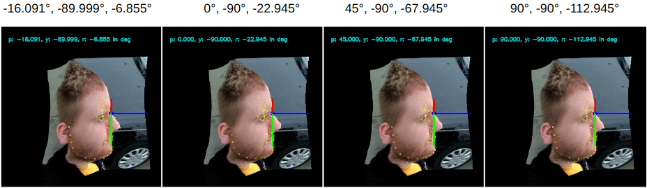
Figure 10: 300W_LP’s Gimbal Lock case.

Furthermore, between the two solutions of yaw, pitch, and roll for the non-gimbal lock case, which one did 300W_LP choose? According to the dataset’s yaw $\in[-90\degree,90\degree]$, and $y_{1}=\bm{arcsin}(-R_{0,2})\in[-90\degree,90\degree]$, we derive that 300W_LP picked the first solution in Listing 22.

6 300W_LP’s three-line drawing: Sec 5.4 v.s. draw_axis() (Listing 26)

Hopenet [7] abandons the traditional approach that entirely relied on landmark detection and then solves the 2D to 3D correspondence problem with a mean human head model. Instead of the extraneous head model and an ad-hoc fitting step, Hopenet determines pose by training its convolutional neural network on the 300W-LP dataset. Its three-line (pose) drawing routine for the 300W_LP dataset is draw_axis() (shown in Listing 26). Since then, this drawing routine has been widely used for many head-pose-estimation papers such as WHENet [8], 6D-RepNet [9], DirectMHP [31] etc.

While draw_axis() is popular and seems to depict three lines well, we still need to prove its drawing correct. Due to our earlier discussion in Section 5.4, we have successfully derived Formula 6. Let’s expand the formula and substitute $R_{W}$ by Formula 5 and $T_{W}$ into $R^{draw}_{W}$. Then we get the following formula:

$$R^{draw}_{W}=\begin{bmatrix}cos(y)cos(r)&-cos(y)sin(r)&-sin(y)\\ cos(p)sin(r)-sin(p)sin(y)cos(r)&cos(p)cos(r)+sin(p)sin(y)sin(r)&-sin(p)cos(y)\\ sin(p)sin(r)+cos(p)sin(y)cos(r)&sin(p)cos(r)-cos(p)sin(y)sin(r)&cos(p)cos(y)\end{bmatrix}.$$ (17)

To project the three columns of $R^{draw}_{W}(p,y,r)$ onto the (image’s) XY-plane, we can reduce the matrix to the following:

$$R^{draw}_{img}(p,y,r)=\begin{bmatrix}cos(y)cos(r)&-cos(y)sin(r)&-sin(y)\\ cos(p)sin(r)-sin(p)sin(y)cos(r)&cos(p)cos(r)+sin(p)sin(y)sin(r)&-sin(p)cos(y)\end{bmatrix},$$ (18)

and the XY-projections for all 3 unit axis vectors are as follows:

$$\begin{split}\bm{x}&=\begin{bmatrix}cos(y)cos(r)\\ cos(p)sin(r)-sin(p)sin(y)cos(r)\end{bmatrix},\bm{y}=\begin{bmatrix}-cos(y)sin(r)\\ cos(p)cos(r)+sin(p)sin(y)sin(r)\end{bmatrix},\bm{z}=\begin{bmatrix}-sin(y)\\ -sin(p)cos(y)\end{bmatrix}\end{split}$$ (19)

To accommodate Line 3’s turning yaw to -yaw in draw_axis() (Listing 26), we replace $cos(y)=cos(-y)$ and $sin(y)=-sin(-y)$ into Formula 19 to get Formula 20. Next, follow Line 3 set $\tilde{y}=-y$ in Formula 20 and we get Formula 21

$$\begin{split}\bm{x^{\prime}}&=\begin{bmatrix}cos(-y)cos(r)\\ cos(p)sin(r)+sin(p)sin(-y)cos(r)\end{bmatrix},\bm{y^{\prime}}=\begin{bmatrix}-cos(-y)sin(r)\\ cos(p)cos(r)-sin(p)sin(-y)sin(r)\end{bmatrix},\bm{z^{\prime}}=\begin{bmatrix}sin(-y)\\ -sin(p)cos(-y)\end{bmatrix};\end{split}$$ (20)

$$\begin{split}\begin{bmatrix}\textrm{x1}\\ \textrm{y1}\end{bmatrix}&=\begin{bmatrix}cos(\tilde{y})cos(r)\\ cos(p)sin(r)+sin(p)sin(\tilde{y})cos(r)\end{bmatrix},\begin{bmatrix}\textrm{x2}\\ \textrm{y2}\end{bmatrix}=\begin{bmatrix}-cos(\tilde{y})sin(r)\\ cos(p)cos(r)-sin(p)sin(\tilde{y})sin(r)\end{bmatrix},\begin{bmatrix}\textrm{x3}\\ \textrm{y3}\end{bmatrix}=\begin{bmatrix}sin(\tilde{y})\\ -sin(p)cos(\tilde{y})\end{bmatrix}.\end{split}$$ (21)

Since Formula 21 completely matches with Lines 15-25 of draw_axis() (Listing 26), we proved draw_axis() equals to our proposed drawing routine (Formula 19).

pose	left	middle	right
pitch	6.208	-17.325	-7.601
yaw	5.876	-49.589	-54.009
roll	-1.694	11.423	4.450

Table 1: 300W_LP’s pose labels for Fig. 11

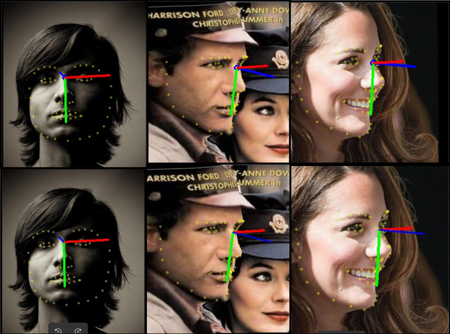
Figure 11: Draw Table 1’s poses with our 300W_LP’s drawing routine (top) and draw_axis (down). Images come from 300W_LP’s HELEN, LFPW, and IBUG datasets. Both methods produce the same outputs.

7 Euler angle Conversion between SciPy’s intrinsic ZYX-order and 300W_LP’s systems

In scenarios such as creating new datasets, adhering to a consistent coordinate system is imperative. A prevalent practice is to employ a popular one such as the 300W_LP or SciPy’s coordinate/rotation system. Consequently, the necessity of performing conversions of Euler angles between these coordinate systems may arise.

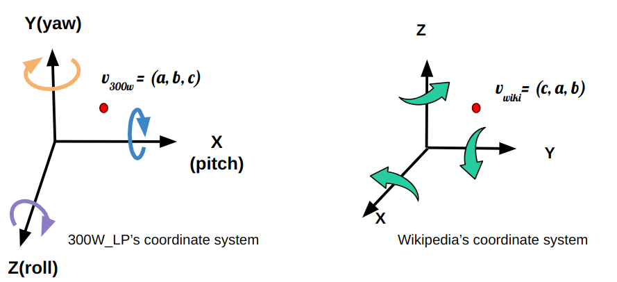
Figure 12: 300W_LP and Wikipedia’s coordinate systems.

7.1 Convert 300W_LP’s rotations into SciPy’s

To convert a 300W_LP’s rotation $R_{W}$ into SciPy’s $R_{S}$, we first substitute a given triple of yaw, pitch, and roll into Formula 5 to obtain $R_{W}$; next apply a coordinate transformation to transform $R_{W}$ of 300W_LP’s coordinate system into its converted rotation matrix, denoted by $\mathbb{T}_{w2s}$, of SciPy’s; and finally compute SciPy’s intrinsic ZYX-order Euler angles through plugging $R_{W}$ into extract_wikiZYX_pose() in Listing 21. Fig. 12 shows the relation between 300W_LP and SciPy’s coordinate systems. So the matrix

$$T_{w2s}\coloneqq\begin{bmatrix}0&0&1\\ 1&0&0\\ 0&1&0\end{bmatrix}$$ (22)

will transform a vector, say $\bm{v}_{300W}=(a,b,c)$, in 300W_LP’s coordinate system into one defined in SciPy’s coordinate system, $\bm{v}_{wiki}=(c,b,a)$. Then $\mathbb{T}_{w2s}$ mentioned earlier can be defined by:

$$\begin{split}\mathbb{T}_{w2s}=T_{w2s}\times R_{W}\times T^{-1}_{w2s}&=\begin{bmatrix}0&0&1\\ 1&0&0\\ 0&1&0\end{bmatrix}\times R_{W}\times\begin{bmatrix}0&0&1\\ 1&0&0\\ 0&1&0\end{bmatrix}\\ &=\begin{bmatrix}0&1&0\\ 0&0&1\\ 1&0&0\end{bmatrix}\times R_{Z}(y)\times R_{Y}(p)\times R_{X}(r)\times\begin{bmatrix}0&1&0\\ 0&0&1\\ 1&0&0\end{bmatrix},\end{split}$$ (23)

where $T_{w2s}$ and $y,p,r,R_{Z},R_{Y},R_{X}$ are defined in Formula 22 and 3 respectively.

7.2 Convert SciPy’s rotations into 300W_LP’s

Similarly, to convert a SciPy’s rotation $R_{S}$ into 300W_LP’s $R_{W}$, we first substitute a given triple of yaw, pitch, and roll into Formula 3 to obtain $R_{S}$; next apply a coordinate transformation, denoted by $\mathbb{T}_{s2w}$ to transform $R_{S}$ of SciPy’s coordinate system into $R_{W}$ of 300W_LP’s; and finally compute 300W_LP’s intrinsic XYZ-order Euler angles through plugging $R_{W}$ into extract_angles_for_300W() in Listing 22. The matrix $T_{s2w}\coloneqq T^{-1}_{w2s}$ will transform a vector, say $\bm{v}_{wiki}=(c,b,a)$, in SciPy’s coordinate system into the vector $\bm{v}_{300W}=(a,b,c)$ in 300W_LP’s coordinate system, Then $\mathbb{T}_{s2w}$ in (2) is defined by:

$$\begin{split}\mathbb{T}_{s2w}&=T_{s2w}\times R_{S}\times T^{-1}_{s2w}\\ &=T^{-1}_{w2s}\times R_{S}\times T_{w2s}\\ &=T^{-1}_{w2s}\times R^{left}_{X}(p)\times R^{left}_{X}(y)\times R^{left}_{Z}(r)\times T_{w2s},\end{split}$$ (24)

where $T_{w2s}$ and $y,p,r,R^{left}_{X},R^{left}_{Y},R^{left}_{Z}$ are defined in Formula 22 and 5 respectively.

7.3 Error measurements for the pose conversion

The conversion of Euler angles between different coordinate/rotation systems inevitably introduces numerical errors. Error/loss measuring can be done directly for poses in the same coordinate system but can’t be directly computed through poses of two different rotation systems. We measure the pose conversion through a matrix norm between the two rotation matrices in the same coordinate system to avoid dealing with different axes-sequences and coordinate systems. So, to compare with the rotation matrix of the first pose, we need to reverse the process described in Sec. 7, transforming the converted pose in the second rotation system back to its equivalent rotation matrix in the first system. The rotation matrices can be measured through the Frobenius or Geodesic norms. Both recognize more subtle differences between rotations. For simplicity, we use the Frobenius norm. Fig. 13 demonstrates our conversions between SciPy and 300W_LP’s poses.

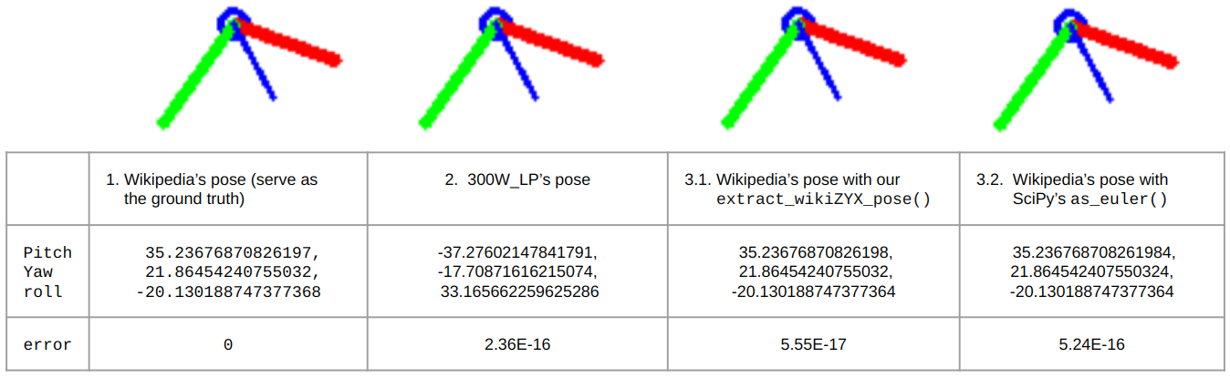
Figure 13: There are 4 different poses in this figure. The first column shows the ground-truth pose (Pose 1) defined in SciPy/Wikipedia’s rotation system. The second column shows the converted pose (Pose 2) in 300W_LP’s rotation system and the Frobenius norm between matrices extracted from Pose 1 and 2 in SciPy’s coordinate system. The third column describes the converted pose (Pose 3.1), which is obtained by calling our extract_wiki_pose(), transformed from Pose 2, and the Frobenius norm between matrices extracted from Pose 1 and 3.1. The last column describes the converted pose (Pose 3.2), which is obtained by calling SciPy’s as_euler(), transformed from Pose 2, and the Frobenius norm between matrices extracted from Pose 1 and 3.2. We used our three-line drawing routines for Wikipedia and 300W_LP’s rotation systems to plot the rotations.

8 Inferring 3DDFA_v2’s rotation system from its implementation [3]

Both 3DDFA [18] and 3DDFA_v2 [32] are the improved versions of the original paper [3], and evaluated 300W-LP based on their implementation. Though sharing the same names, the 3DDFA, an abbreviation of the paper [18], is not the algorithm 3DDFA mentioned in [3]. Their implementations are similar: first, apply Dlib or FaceBoxes [33] face detectors to extract the regions of heads, then infer the 3DMM parameters from the pre-trained models for each bounding region. To achieve fast inference, 3DDFA v2 clips the 3DMM [2] model parameters, $\mathbf{\alpha_{id}}\in\mathbb{R}^{199}$ and $\mathbf{\alpha_{exp}}\in\mathbb{R}^{29}$, into the first 40 and 10 dimensions respectively, and reduces the parameters to ${\mathbf{p}=[T^{3\times 4},\mathbf{\alpha}^{50}]}$. In the following sub-section, we’ll explain how $T^{3\times 4}$ works.

3DDFA_v2 [32] uses the 300W-LP dataset in its experiments. So, to derive 3DDFA_v2’s Euler angles for the 300W-LP dataset, we carefully examined its implementation [3] and found out that, for each detected bounded box, the pre-trained TDDFA model will output $T^{3\times 4}$. $T^{3\times 4}$ then can be decomposed into a 3x3 rotation matrix, $R_{W^{\prime}}$, a scaling factor $s$, and a translation offset $t3d$. We denote 3DDFA_v2’s rotation matrix by $R_{W^{\prime}}$ in case this definition is different from 300W_LP’s $R_{W}$ notation. We notice that 3DDFA_v2 applies the pose frustum drawing scheme discussed in Sec. 5.3 (See Fig. 9) without really using its yaw, roll, pitch values.

The function matrix2angle() in 3DDFA_v2/utils/pose.y (shown in Listing 23) is the only source code to provide the yaw-roll-pitch extraction for $R_{W^{\prime}}$. The discussion about the Base Face Model (BFM) in Sec. 5.2 implies both 3DDFA and 3DDFA_v2 and 300W_LP share the same coordinate system. Don’t be misled by the phrase, x(yaw), y(pitch), and z(roll), in matrix2angle()’s Docstrings because they don’t mean the associated rotation really rotating along the X-, Y-, and Z-axes respectively.

The non-gimbal-lock case (Lines 23-25) of matrix2angle() encourages the first column and first row of $R_{W^{\prime}}$ to follow the pattern (25) where $y,p,r$ means yaw, pitch and roll respectively:

$$R_{W^{\prime}}(y,p,r)=\begin{bmatrix}cos(r)cos(y)&-&-\\ sin(r)cos(y)&-&-\\ sin(y)&cos(y)sin(p)&cos(y)cos(p)\end{bmatrix}$$ (25)

Because each Euler angle rotates along one of the X-, Y-, or Z-axes and different Euler angles rotate along different axes, the three fundamental rotation matrices associated with yaw, roll, and pitch have the zero-one column and row distributions (See (26)). Once the zero-one pattern is fixed for one Euler angle, say yaw, the other Euler angles won’t have the same zero-one pattern. All possible fundamental rotation matrices are shown in (27).

$$\begin{bmatrix}1&0&0\\ 0&-&-\\ 0&-&-\end{bmatrix},\begin{bmatrix}-&0&-\\ 0&1&0\\ -&0&-\end{bmatrix},\begin{bmatrix}0&0&1\\ -&-&0\\ -&-&0\end{bmatrix}$$ (26)

$$\begin{bmatrix}1&0&0\\ 0&cos(\theta)&\mp sin(\theta)\\ 0&\pm sin(\theta)&cos(\theta)\end{bmatrix},\begin{bmatrix}cos(\theta)&0&\pm sin(\theta)\\ 0&1&0\\ \mp sin(\theta)&0&cos(\theta)\end{bmatrix},\begin{bmatrix}cos(\theta)&\mp sin(\theta)&0\\ \pm sin(\theta)&cos(\theta)&0\\ 0&0&1\\ \end{bmatrix}$$ (27)

We compute the yaw-roll-pitch rotation matrices from all possible fundamental rotation matrix multiplications to find the solutions for $R_{W^{\prime}}(y,p,r)$ with the given pattern (25) used in 3DDFA_v2. Among all $\pm$ y, $\pm$p, $\pm$r, X, Y, Z choices, there’s one unique solution found (Formula (29)), and we use the notation $R^{right}_{Z}(r)$ to represent the roll rotation along the Z-axis in the right-handed manner in 300W_LP’s coordinate system.

$$R^{right}_{X}(p)=\begin{bmatrix}1&0&0\\ 0&cos(p)&-sin(p)\\ 0&sin(p)&cos(p)\end{bmatrix},\\ R^{left}_{Y}(y)=\begin{bmatrix}cos(y)&0&-sin(y)\\ 0&1&0\\ sin(y)&0&cos(y)\end{bmatrix},R^{right}_{Z}(r)=\begin{bmatrix}cos(r)&-sin(r)&0\\ sin(r)&cos(r)&0\\ 0&0&1\end{bmatrix},$$ (28)

$$\begin{split}R^{{}^{\prime}}_{W}(y,p,r)&=R^{right}_{Z}(r)\times R^{lefft}_{Y}(y)\times R^{right}_{X}(p)\\ &=\begin{bmatrix}cos(r)cos(y)&-sin(p)sin(y)cos(r)-sin(r)cos(p)&sin(p)sin(r)-sin(y)cos(p)cos(r)\\ sin(r)cos(y)&-sin(p)sin(r)sin(y)+cos(p)cos(r))&-sin(p)cos(r)-sin(r)sin(y)cos(p)\\ sin(y)&sin(p)cos(y)&cos(p)cos(y)\end{bmatrix}\end{split}$$ (29)

So we show that Formula (29) is the unique solution to Eq. (25). Comparing 3DDFA and 3DDFA_v2’s $R^{{}^{\prime}}_{W}(y,p,r)=R^{right}_{Z}(r)\times R^{lefft}_{Y}(y)\times R^{right}_{X}(p)$ with 300W_LP’s $R_{W}(y,p,r)=R^{left}_{X}(p)\times R^{left}_{Y}(y)\times R^{left}_{Z}(r)$, we proved that 3DDFA and 3DDFA_v2 uses different axis-sequence and handedness from 300W_LP’s.

To align with 300W_LP’s rotation system and adjust matrix2angle’s errors, we suggest applying the rotation formula $R_{W}$ in Formula 5, the pose extraction from Listing 22, and one of the 300W_LP’s drawing routines mentioned in Sec 5.4.

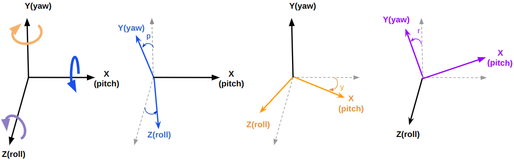
Figure 14: matrix2angle defines mix-handed elemental rotations

9 Head pose estimation: 6D-RepNet [9] and 6D-RepNet360 [10]

6D-RepNet uses a network RepVGG [34], allowing skip-connection-like structure during training time while the skip connections are merged into conv-net operation during inference. Deep learning generates features by itself, so there is no need for key-point detection. Both 6D-RepNet and 6D-RepNet360 introduce a 6D representation as the neural network’s output. Subsequently, the Gram-Schmidt process is employed to construct a rotation matrix from the 6D representation, with learning facilitated through the geodesic loss of rotation matrices. However, both 6D-RepNets’ papers [9] and [10] lack explicit statements about its rotation system used to train/test with 300W-LP alone or combining with CMU Panoptic. Since there’s no coordinate transformation involved, we can only assume 6D-RepNet inherits 300W_LP’s coordinate system as it is training directly with 300W_LP’s ground truth labels.

Both 6D-RepNets interpret the yaw, roll, and pitch from the predicted rotation matrix through the function shown in Listing 25. Then, plot the Euler angles with the three-line and pose-box drawing routines, as shown in Listing 26 and 27. We must consider them all to unveil 6D-RepNet’s rotation system and Euler angle definitions.

9.1 6D-RepNet’s rotation system vs 300W_LP’s: are they the same?

Let’s start with its drawing routines, draw_axis() in Listing 26 and plot_pose_cube() in Listing 27. Because plot_pose_cube() follows draw_axis()’s logic, we only need to consider draw_axis(). Sec. 6 has shown that draw_axis()’s three lines (Formula 18) correspond to

$$\begin{split}R^{draw}_{img}(p,y,r)&=\begin{bmatrix}1&0&0\\ 0&1&0\end{bmatrix}\times R^{draw}_{W}(p,y,r)\\ &=\begin{bmatrix}cos(y)cos(r)&-cos(y)sin(r)&-sin(y)\\ cos(p)sin(r)-sin(p)sin(y)cos(r)&cos(p)cos(r)+sin(p)sin(y)sin(r)&-sin(p)cos(y)\end{bmatrix}.\end{split}$$ (30)

Lemma 9.1.

$R^{draw}_{W}(p,y,r)$ is the only rotation matrix satisfying

$$R^{draw}_{img}=\begin{bmatrix}1&0&0\\ 0&1&0\end{bmatrix}\times R,\quad where\,\;R\,\;is\,\;a\,\;3\times 3\,\;rotation\,\;matrix.$$ (31)

Proof.

Since $R^{draw}_{W}(p,y,r)$ is the rotation matrix (check Sec. 5.4), and let $\vec{a}$ and $\vec{b}$ represent the first and second rows of $R^{draw}_{W}(p,y,r)$, $\vec{a}$ and $\vec{b}$ must be orthonormal. The fact of $R$’s determinant $=1$ leads to the third row of $R$ equal to the cross product of $\vec{a}$ and $\vec{b}$, i.e., $\vec{a}\times\vec{b}$. So, we proved that only one unique rotation matrix satisfies Eq. 31. Then $R=R^{draw}_{W}(p,y,r)$. ∎

Combining Lemma 9.1 with Formula 6, we can derive 6D-RepNet’s rotation, denoted by $R^{*}_{6d}$, equals $R_{W}$ as shown below .

$$\begin{split}R^{*}_{6d}&=T^{-1}_{W}\times R^{draw}_{W}(p,y,r)\times T_{W}=R_{W}\\ \implies R^{*}_{6d}&=R_{W}=R^{left}_{X}(p)\times R^{left}_{Y}(y)\times R^{left}_{Z}(r).\end{split}$$ (32)

Thus draw_axis() completely follows 300W_LP’s rotation system.

Next, let’s dive into 6D-RepNet’s rotation matrix formula, Formula 33 and 34 implemented in get_R() (check Listing 25 for details).

$$R^{right}_{X}(p)=\begin{bmatrix}1&0&0\\ 0&cos(p)&-sin(p)\\ 0&sin(p)&cos(p)\end{bmatrix},\\ R^{right}_{Y}(y)=\begin{bmatrix}cos(y)&0&sin(y)\\ 0&1&0\\ -sin(y)&0&cos(y)\end{bmatrix},R^{right}_{Z}(r)=\begin{bmatrix}cos(r)&-sin(r)&0\\ sin(r)&cos(r)&0\\ 0&0&1\end{bmatrix},$$ (33)

$$\begin{split}R^{**}_{6d}(y,p,r)&=R^{right}_{Z}(r)\times R^{right}_{Y}(y)\times R^{right}_{X}(p)\\ &=\begin{bmatrix}cos(r)cos(y)&sin(p)sin(y)cos(r)-sin(r)cos(p)&sin(p)sin(r)+sin(y)cos(p)cos(r)\\ sin(r)cos(y)&sin(p)sin(r)sin(y)+cos(p)cos(r)&-sin(p)cos(r)+sin(r)sin(y)cos(p)\\ -sin(y)&sin(p)cos(y)&cos(p)cos(y)\end{bmatrix}\end{split}$$ (34)

It shows another rotation matrix formula, denoted as $R^{**}_{6d}$, $R^{**}_{6d}=R^{right}_{Z}(r)\times R^{right}_{Y}(y)\times R^{right}_{X}(p)$ , which contradicts $R^{*}_{6d}$ of Formula 32. Therefore, 6D-RepNet applies 2 rotation systems defined in 300W_LP’s coordinate system, $R^{**}_{6d}$ for head pose dataset retrieval/training/inference, $R^{*}_{6d}$ for the drawing purpose. Luckily, we notice that $R_{W}$ and $R^{**}_{6d}(y,p,r)$ are inverse of each other, i.e.,

$$\begin{split}R^{**}_{6d}(y,p,r)&=R^{right}_{Z}(r)\times R^{right}_{Y}(y)\times R^{right}_{X}(p)\\ \ &=R^{left}_{Z}(-r)\times R^{left}_{Y}(-y)\times R^{left}_{X}(-p)\\ &=(R^{left}_{X}(p)\times R^{left}_{Y}(y)\times R^{left}_{Z}(r))^{-1}\\ &=R_{W}(y,p,r)^{-1}\\ &=R_{W}(y,p,r)^{transpose}.\end{split}$$ (35)

The above derivation implies two observations. Firstly, 6D-RepNet’s neural network learning with $R^{**}_{6d}(y,p,r)$-rotations still works because the Geodesic distance (used in 6D-RepNet’s training) between two $R^{**}_{6d}$-rotations remains the same as the Geodesic distance between their inverse rotations, i.e., $R_{W}$-rotations. Secondly, draw_axis() works for 6D-RepNet’s Euler-angle predictions because $R^{**}_{6d}$’s predicted pitch, yaw, roll also remain the same as $R_{W}$’s according to Equality 35.

Finally, we notice that 6D-RepNet’s Euler angle extraction, shown in Listing 24, only outputs one set of pitch, yaw, and roll. As discussed at the end of Sec. 5.5, if we can show yaw $\in[-90\degree,90\degree]$, then 6D-RepNet and 300W_LP share the same pose selection. Because Listing 24’s Line 7’s $sy=|cos(yaw)|$ forces Line 12, $y=torch.atan2(-R[:,2,0],sy)$, to output yaw $\in[-90\degree,90\degree]$, 6D-RepNet and 300W_LP indeed share the same pose selection (the first one as in Listing 22).

9.2 Conclusion

6D-RepNet adapts 300W_LP’s inverse rotation system. So, while its predicted rotation matrices don’t align with 300W_LP’s rotation system, its extracted Euler angles coincide with 300W_LP’s Euler angles. Hence, we can plot the predicted 300W_LP’s rotations correctly by plugging the predicted Euler angles into draw_axis().

10 WHENet’s head pose generation

To train its HPE model, WHENet [8] follows the convention of training with 300W_LP and testing with AFLW2000 [3] and BIWI [35]. Although 300W_LP contains 150K images, it lacks images with yaws close to 0 or outside of the angle range $[-90\degree,90\degree]$. On the other hand, the CMU Panoptic Dataset [19] captures multiple (occlusive) subjects from an abundance of calibrated cameras covering a full hemisphere and provides facial landmarks in 3D. WHENet, as far as we can tell, was the first to propose an open-sourced code for their pose extraction method, implemented in prepare_images.py (Listing 28), for the CMU Panoptic Dataset [19]. They estimated head pose from the provided facial keypoints and calculated rotations to go from the standard-pose face model to it using Horn’s closed-form formula [36]. WHENet then combines the frontal-poses and anterior-view pose labels from 300W_LP and CMU Panoptic Datasets to construct a more balanced head pose dataset with the desired full-pose-range coverage.

WHENet [8] also uses draw_axis() (Listing 26) for three-line drawing. As discussed in Sec. 9, draw_axis is tailored for the Euler angles from 300W_LP’s rotation system. So, the rest of this section will focus on whether WHENet’s head pose generation for CMU Panoptic Dataset follows 300W_LP’s rotation system.

10.1 The head pose generation for CMU Panoptic Dataset

The head pose generation is implemented in the function save_img_head(), i.e., Listing 28, and needed to be examined.

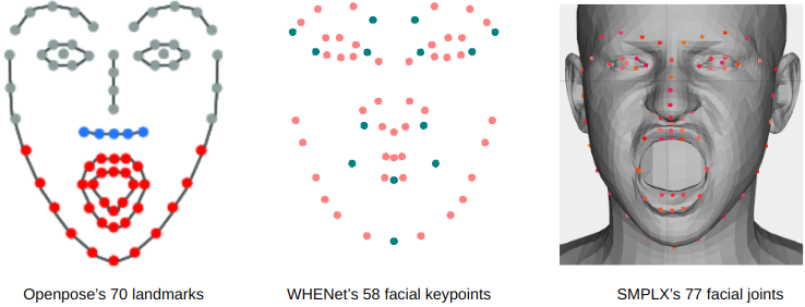
Figure 15: From left to right: Openpose’s 70 lanmarks, WHENet’s 58-keypoint BFM, and SMPLX’s [37] 77 face joints.

10.1.1 WHENet adapts 300W_LP’s rotation system

CMU Panoptic Dataset uses OpenPose’s [38] 70 facial landmarks [39] to define each individual’s unique 3D face. Due to no corresponding face model for the standard pose( i.e., pose with yaw=pitch=roll=0), WHNENet uses the 58-keypoint face model $X_{ref}$ defined by Listing 31 to represent the standard-pose face model(the middle in Fig. 15). Due to the landmark difference, WHENet picks 6-14 keypoints (green dots in Fig. 15) and applies Horn’s closed-form solution [36] to estimate the rotation $R_{Horn}$ (i.e., $temp$ in the code) from the keypoints to the corresponding CMU Panoptic Dataset’s ground-truths. For simplicity, we assume $R_{Horn}$ is $3\times 3$. Moreover, while $X_{ref}$ follows 300W_LP’s rotation system (left in Fig. 5), yet OpenPose’s standard-pose landmarks turn $180\degree$ along the X-axis. So to eliminate the impact and transform the corrected rotation matrix into the image’s(i.e., 300W_LP’s) 3D coordinate system through the ground-truth camera’s extrinsic $C_{extr}$, we derive WHENet’s rotation is shown as follows:

$$R=\begin{bmatrix}1&0&0\\ 0&-1&0\\ 0&0&-1\end{bmatrix}\times C_{extr}\times R_{Horn}\times\begin{bmatrix}1&0&0\\ 0&-1&0\\ 0&0&-1\end{bmatrix}^{-1},\;where\;C_{extr}=cam[R]\;in\;Listing\;\ref{listing:11}$$ (36)

Lines 28-30 in Listing 28 tell us how WHENet transforms the camera’s rotation into the one in 300W-LP’s. From the Euler angle extraction code (Listing 29), we derive the rotation has the form:

$$R_{wh}(y,p,r)=\begin{bmatrix}cos(y)cos(r)&cos(y)sin(r)&-sin(y)\\ -cos(p)sin(r)+sin(p)sin(y)cos(r)&cos(p)cos(r)+sin(p)sin(y)sin(r)&sin(p)cos(y)\\ sin(p)sin(r)+cos(p)sin(y)cos(r)&-sin(p)cos(r)+cos(p)sin(y)sin(r)&cos(p)cos(y)\end{bmatrix}.$$ (37)

We find Formula 37’s $R_{wh}(y,p,r)$ is the same as 300W_LP’s $R_{W}$(in Formula 5). Listing 27’s lines 29-30 (turning yaw and roll to be negative) correspond to the first left matrix (not $R$) shown in Formula 36. The function, select_euler(), of Listing 29 shows WHENet forces the pitch and roll values $\in[-90\degree,90\degree]$ and may make yaw beyond $\pm 90\degree$ . If one of pitch or roll is out of this range, -999 will be assigned to yaw, pitch, and roll. So, WHENet adapts 300W_LP’s rotation system except for the Euler angle selection (in the sense of which output from Listing 22).

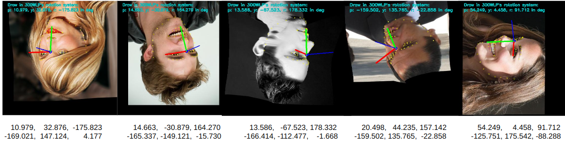
Figure 16: The bottom 2 rows are the complete (pitch, yaw, roll) solutions for the above images. The first row has yaw values $\in[-90\degree,90\degree]$, and the second row has yaw values beyond $\pm 90\degree$. If we pass the rotation matrices into 6D-RepNet and WHENet’s Euler angle extractions, they will output the top row and $(-999,-999,-999)$, respectively.

10.1.2 Rotations: WHENet v.s. 300W_LP

Unlike WHENet using $X_{ref}$ to represent the standard-pose face model for all faces of various shapes and expressions, 300W_LP’s FP-perturbation scheme applies the 3DDFA algorithm focusing on each individual’s facial shape and expression to reduce the fitting errors: first transforms the BFM($\bar{S}$) in Fig. 6, with the shape and expression parameters, to the standard face model $S$ which aligns to the non-rotated face model, and then compute the rotation from $S$ to the rotated 3D face. We believe that applying certain FP-perturbation schemes before performing the rotation calculation in Sec.10.1.1 would enhance precision for HPE.

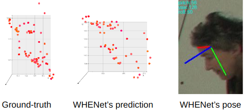
Figure 17: This figure illustrates WHENet’s predicted face (middle) based on a ground-truth face model (left). The right shows the predicted rotation. The red line should stretch to the right, not the left, so the predicted pose is not desired.

10.2 The head pose generation for the AGORA dataset [40]

AGORA [40] is a synthetic dataset which places various SMPL-X [37] body models on realistic 3D environments. It has around 14K training and 3K test images, rendering between 5 and 15 people per image using image-based lighting or rendered 3D environments. In total, AGORA consists of 173K person crops. When we carefully compared DirectMHP’s (DMHP) [31]’s head pose generation for the AGORA dataset, auto_labels_generating() (shown in Listing 30) with WHENet’s save_img_head()(Listing 28), we found DMHP only made three changes: (1) it rotates $X_{ref}$ along X-axis by 10 °with left-handed rule, and treat it, denoted by $H_{ref}$, as its universal standard face model; (2) it picks 13 out of the 58 keypoints in $H_{ref}$ to match with SMPLX’s 13 out of the selected 51 face joints; and (3) the head region’s sanity check is tailored for AGORA’s faces. Therefore, we conclude that DMHP adapts WHENet’s rotation system and Euler angle extraction.

11 2D image data augmentation for head pose dataset

In this section, we will focus on the standard 2D geometric image augmentation commonly employed in deep-learning-based image classification, such as rotations/flipping and their effects on rotation matrices. Data augmentation is a crucial tool in the training pipeline for computer vision models, enabling them to achieve higher performance, improved generalization, and greater robustness without increasing the number of training images. However, in HPE, geometric image augmentations have been avoided due to a lack of clear definition of rotation systems and mathematical derivation of new rotation matrices under 2D geometric transformation. Clearly, geometrical transformation also enhances angle coverage for free.

It is easy to observe that pixel-level image augmentations do not alter the rotation matrices. Readers can easily compute the Euler angles with knowledge from Sec. 5.5 when the correct rotation matrices are available.

Definition 11.1.

The 2D images are assumed to be on the $XY$-plane of the 300W_LP’s coordinate system as in Figure 5. 2D images’ horizontal & vertical flipping are the flipping across the image’s vertical Y-axis and horizontal X-axis, respectively. And a image’s rotation with the angle $\bm{\phi}$ is the rotation rotating the image an angle, $\phi$, clockwise or counter-clockwise, which is decided by the rotation system. In 300W_LP’s and Wikipedia’s systems, the angle $\phi$ represents rotating $\phi$ clockwise and counter-clockwise, respectively.

Definition 11.2.

Define $\bm{L_{\theta}}$ to be the line passing through the origin and the angle from the horizontal axis and itself (on the vertical plane, denoted by $\bm{P_{v}}$, intersecting with the horizontal and vertical axes) is $\theta$. For example, the line $L_{\theta}$ of 300W_LP’s coordinate system represents one constructed from rotating the X-axis ($y=0$) by the angle $\theta$ counter-clockwise on the XY-plane. Because of 300W_LP’s left-handed nature for the XY-plane’s rotations, such rotations are clockwise. So $\theta>0$ is equivalent to the roll rotation $r=-\theta$ in 300W_LP’s rotation system. However, Wikipedia’s rotation system’s right-handed nature guarantees its roll rotation $r=\theta$ will remain the same sign as $L_{\theta}$’s $\theta$.

Definition 11.3.

Next, we define the 2D flipping about $\bm{L_{\theta}}$ to be the flipping across $L_{\theta}$ on the vertical plane $\bm{P_{v}}$ defined in Definition 11.2.

We will derive formulas under 300W_LP’s coordinate system and conventions. Similar derivations can be carried out easily for other coordinate systems.

Theorem 11.4.

Fix a 3D rotation system. Suppose an image contains a human head, and the head’s intrinsic rotation $R$ in the rotation system is given. Prove that the 3D rotation, denoted by $R_{rotate{\_}img}(\phi)$, associated with rotating this image by an angle $\phi$ is the same to apply the extrinsic rotation, denoted as $R_{extr}(\phi)$, of rotating the axis (perpendicular to the image) by the angle $\phi$ on $R$. Hence, we have

$$R_{rotate{\_}img}(\phi)=R_{extr}(\phi)\times R$$ (38)

Proof.

Without loss of generality, let’s fix to 300W_LP’s rotation system and $R\neq I_{3}$. So, rotating the image by $\phi$ clockwise results in the roll’s elemental rotation $R^{left}_{Z}(\phi)$ defined in Formula 5. The roll’s elemental rotation is extrinsic because the image’s rotation can only happen on 300W_LP’s extrinsic $xy$-plane. Then we apply Lemma 3.3 and can derive that $R_{rot{\_}img}(\phi)$ satisfies Formula 39.

$$\begin{split}&R_{extr}(\phi)=R^{left}_{Z}(\phi),\\ &R_{rot{\_}img}(\phi)=R_{extr}(\phi)\times R=R^{left}_{Z}(\phi)\times R\\ \implies&R_{rot{\_}img}(\phi)=\begin{bmatrix}cos(\phi)&sin(\phi)&0\\ -sin(\phi)&cos(\phi)&0\\ 0&0&1\end{bmatrix}\times R\end{split}$$ (39)

∎

Theorem 11.5.

Let’s fix 300W_LP’s rotation system and restrict $\theta\leq 90\degree$. Suppose an image contains a human head, and the head’s intrinsic rotation $R$ in the fixed rotation system is given. Prove that the 3D rotation $R_{flip}(\theta)$, corresponding to the 2D flipping across $L_{\theta}$ and the given head’s rotation $R$, can be expressed as follows:

$$R_{flip}(\theta)=\begin{bmatrix}cos(2\theta)&sin(2\theta)&0\\ sin(2\theta)&-cos(2\theta)&0\\ 0&0&1\end{bmatrix}\times R\times\begin{bmatrix}-1&0&0\\ 0&1&0\\ 0&0&1\end{bmatrix}$$ (40)

Proof.

Without loss of generality, let $R\neq I_{3}$. It’s trivial that the 2D flipping across $L_{\theta}$ will flip from $\bm{e_{x}}\coloneqq(1,0,0)$ to $(cos(2\theta),sin(2\theta),0)$. But the 2D flipping across $L_{\theta}$ flips $\bm{e_{y}}\coloneqq(0,1,0)$ to $(sin(2\theta),-cos(2\theta),0)$ requires some work. So the matrix of the extrinsic 3D flipping is $\begin{bmatrix}cos(2\theta)&sin(2\theta)&0\\ sin(2\theta)&-cos(2\theta)&0\\ 0&0&1\end{bmatrix}$. The flipping also causes the intrinsic X-axis to change to the opposite direction, which results in the intrinsic flipping across the X-axis, i.e., $\begin{bmatrix}-1&0&0\\ 0&1&0\\ 0&0&1\end{bmatrix}$. Therefore, the 2D flipping across $L_{\theta}$ relates to the 3D rotation, which applies an extrinsic $L_{\theta}$-flipping and an intrinsic $X$-flipping. By Lemma 3.3, we have $R_{flip}(\theta)=(extrinsic{\_}L_{\theta}{\_}flipping)\times R\times(intrinsic{\_}X{\_}flipping)$, and thus proved Formula 40. ∎

Corollary 11.5.1.

Here we list a few special cases of the above theorem under 300W_LP’s rotation system:

1. Horizontal flipping is $R_{flip}(\pi/2)=\begin{bmatrix}-1&0&0\\ 0&1&0\\ 0&0&1\end{bmatrix}\times R\times\begin{bmatrix}-1&0&0\\ 0&1&0\\ 0&0&1\end{bmatrix}$.

2. Vertical flipping is $R_{flip}(0)=\begin{bmatrix}1&0&0\\ 0&-1&0\\ 0&0&1\end{bmatrix}\times R\times\begin{bmatrix}-1&0&0\\ 0&1&0\\ 0&0&1\end{bmatrix}$.

3. Flipping about both axes is $R_{bf}=\begin{bmatrix}-1&0&0\\ 0&1&0\\ 0&0&1\end{bmatrix}\times\begin{bmatrix}1&0&0\\ 0&-1&0\\ 0&0&1\end{bmatrix}\times R\times\begin{bmatrix}-1&0&0\\ 0&1&0\\ 0&0&1\end{bmatrix}\times\begin{bmatrix}-1&0&0\\ 0&1&0\\ 0&0&1\end{bmatrix}=\begin{bmatrix}-1&0&0\\ 0&-1&0\\ 0&0&1\end{bmatrix}\times R.$

4. The symmetrical flipping about $\bm{L_{\pi/4}}$ is $R_{flip}(\pi/4)=\begin{bmatrix}0&1&0\\ 1&0&0\\ 0&0&1\end{bmatrix}\times R\times\begin{bmatrix}-1&0&0\\ 0&1&0\\ 0&0&1\end{bmatrix}.$

5. The rotation $\pi/4$ counter-clockwise corresponds to $R_{rd}=\begin{bmatrix}0&1&0\\ 1&0&0\\ 0&0&1\end{bmatrix}\times R$.

Fig. 18 demonstrates Corollary 11.5.1 applied to various head pose images.

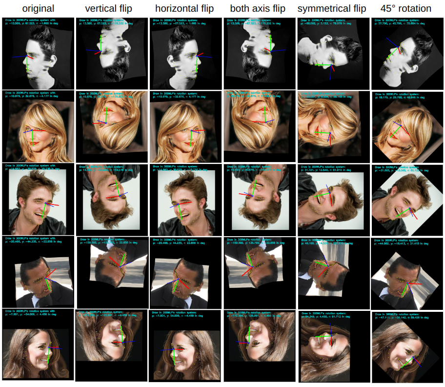
Figure 18: Our pose & rotation augmentations for the 300W_LP dataset

Figure 19: 300W_LP’s Gimbal-lock images: Euler angles follows pitch, yaw, and roll order.

⬇

y, p, r = rot_mtx.as_euler(’ZYX’, degrees=True)

Figure 20: SciPy’s Euler angle extraction

⬇

import numpy as np

from np import arcsin, pi, arctan2, cos, sin, ndarray

\pardef extract_wikiZYX_pose(R_wiki: ndarray((3,3)):

if np.abs(R_wiki[2, 0]) != 1.:

p1 = -arcsin(R_wiki[2, 0])

p2 = pi - p1 if p1 >= 0 else -pi - p1

cp1 = cos(p1)

r1 = arctan2(R_wiki[2, 1] / cp1, R_wiki[2, 2] / cp1)

r2 = (r1 - pi) if r1 >= 0. else (r1 + pi)

y1 = arctan2(R_wiki[1, 0] / cp1, R_wiki[0, 0] / cp1)

y2 = (y1 - pi) if y1 >= 0. else (y1 + pi)

\parreturn (p1, y1, r1), (p2, y2, r2)

else:

if R_wiki[2, 0] == -1:

p = pi / 2

r = arctan2(R_wiki[0, 1], R_wiki[0, 2]) / 2

y = -r

else:

p = -pi / 2

y = r = arctan2(-R_wiki[0, 1], -R_wiki[0, 2]) / 2

return (p, y, r), None

Figure 21: Complete yaw, roll, pitch formula for Wikipedia’s right-handed intrinsic ZYX-sequence rotations

⬇

import numpy as np

from np import arcsin, pi, arctan2, cos, sin, ndarray

\pardef extract_euler_angles_for_300W(R: ndarray((3,3)):

half_pi = pi / 2

y1 = arcsin(-R[0,2])

if y1 == half_pi:

p = arctan2(R[1,0], R[1,1]) / 2

r = -p

return (p, y1, r)

elif y1 == -half_pi:

p = r = arctan2(-R[1,0], R[1,1]) / 2

return (p, y1, r)

else: # non-Gimbal-lock cases

cy1 = cos(y1)

y2 = (pi - y1) if y1 >= 0 else (-pi - y1)

p1 = arctan2(R[1,2] / cy1, R[2,2] / cy1 )

p2 = (p1 - pi) if p1 >= 0 else (p1 + pi)

r1 = arctan2(R[0,1] / cy1, R[0,0] / cy1)

r2 = (r1 - pi) if r1 >= 0 else (r1 + pi)

return (p1, y1, r1), (p2, y2, r2)

Figure 22: Complete yaw, roll, pitch formula for the 300W-LP dataset

⬇

def matrix2angle(R):

""" compute three Euler angles from a Rotation Matrix. Ref:

http://www.gregslabaugh.net/publications/euler.pdf

refined by: https://stackoverflow.com/questions/43364900/

rotation-matrix-to-euler-angles-with-opencv

todo: check and debug

Args:

R: (3,3). rotation matrix

Returns:

x: yaw

y: pitch

z: roll

"""

if R[2, 0] > 0.998:

z = 0

x = np.pi / 2

y = z + atan2(-R[0, 1], -R[0, 2])

elif R[2, 0] < -0.998:

z = 0

x = -np.pi / 2

y = -z + atan2(R[0, 1], R[0, 2])

else:

x = asin(R[2, 0])

y = atan2(R[2, 1] / cos(x), R[2, 2] / cos(x))

z = atan2(R[1, 0] / cos(x), R[0, 0] / cos(x))

\parreturn x, y, z

Figure 23: 3DDFA and 3DDFA_v2’s matrix2angle() function

⬇

#input batch*4*4 or batch*3*3

#output torch batch*3 x, y, z in radiant

#the rotation is in the sequence of x,y,z

def compute_euler_angles_from_rotation_matrices(rotation_matrices):

batch = rotation_matrices.shape[0]

R = rotation_matrices

sy = torch.sqrt(R[:,0,0]*R[:,0,0]+R[:,1,0]*R[:,1,0])

singular = sy<1e-6

singular = singular.float()

\parx = torch.atan2(R[:,2,1], R[:,2,2])

y = torch.atan2(-R[:,2,0], sy)

z = torch.atan2(R[:,1,0],R[:,0,0])

\parxs = torch.atan2(-R[:,1,2], R[:,1,1])

ys = torch.atan2(-R[:,2,0], sy)

zs = R[:,1,0]*0

\pargpu = rotation_matrices.get_device()

if gpu < 0:

out_euler = torch.autograd.Variable(torch.zeros(batch,3)).to(torch.device(’cpu’))

else:

out_euler = torch.autograd.Variable(torch.zeros(batch,3)).to(torch.device(’cuda:out_euler[:,0] = x*(1-singular)+xs*singular

out_euler[:,1] = y*(1-singular)+ys*singular

out_euler[:,2] = z*(1-singular)+zs*singular

\parreturn out_euler

Figure 24: 6D-RepNet/6D-RepNet360’s Euler angle extraction code

⬇

def get_R(x,y,z):

”’ Get rotation matrix from three rotation angles (radians). right-handed.

Args:

angles: [3,]. x, y, z angles

Returns:

R: [3, 3]. rotation matrix.

”’

# x

Rx = np.array([[1, 0, 0],

[0, np.cos(x), -np.sin(x)],

[0, np.sin(x), np.cos(x)]])

# y

Ry = np.array([[np.cos(y), 0, np.sin(y)],

[0, 1, 0],

[-np.sin(y), 0, np.cos(y)]])

# z

Rz = np.array([[np.cos(z), -np.sin(z), 0],

[np.sin(z), np.cos(z), 0],

[0, 0, 1]])

\parR = Rz.dot(Ry.dot(Rx))

return R

Figure 25: 6D-RepNet/6D-RepNet360’s rotation matrix formula

⬇

def draw_axis(img, yaw, pitch, roll, tdx=None, tdy=None, size = 100):

pitch = pitch * np.pi / 180

yaw = -(yaw * np.pi / 180)

roll = roll * np.pi / 180

\parif tdx != None and tdy != None:

tdx = tdx

tdy = tdy

else:

height, width = img.shape[:2]

tdx = width / 2

tdy = height / 2

\par# X-Axis pointing to right. drawn in red

x1 = size * (cos(yaw) * cos(roll)) + tdx

y1 = size * (cos(pitch) * sin(roll) + cos(roll) * sin(pitch) * sin(yaw)) + tdy

\par# Y-Axis | drawn in green

# v

x2 = size * (-cos(yaw) * sin(roll)) + tdx

y2 = size * (cos(pitch) * cos(roll) - sin(pitch) * sin(yaw) * sin(roll)) + tdy

\par# Z-Axis (out of the screen) drawn in blue

x3 = size * (sin(yaw)) + tdx

y3 = size * (-cos(yaw) * sin(pitch)) + tdy

\parcv2.line(img, (int(tdx), int(tdy)), (int(x1),int(y1)),(0,0,255),4)

cv2.line(img, (int(tdx), int(tdy)), (int(x2),int(y2)),(0,255,0),4)

cv2.line(img, (int(tdx), int(tdy)), (int(x3),int(y3)),(255,0,0),4)

\parreturn img

Figure 26: HopeNet/WHENet/6D-RepNet/6D-RepNet360’s three-line drawing routine

⬇

def plot_pose_cube(img, yaw, pitch, roll, tdx=None, tdy=None, size=150.):

# Input is a cv2 image

# pose_params: (pitch, yaw, roll, tdx, tdy)

# Where (tdx, tdy) is the translation of the face.

# For pose we have [pitch yaw roll tdx tdy tdz scale_factor]

\parp = pitch * np.pi / 180

y = -(yaw * np.pi / 180)

r = roll * np.pi / 180

if tdx != None and tdy != None:

face_x = tdx - 0.50 * size

face_y = tdy - 0.50 * size

\parelse:

height, width = img.shape[:2]

face_x = width / 2 - 0.5 * size

face_y = height / 2 - 0.5 * size

\parx1 = size * (cos(y) * cos(r)) + face_x

y1 = size * (cos(p) * sin(r) + cos(r) * sin(p) * sin(y)) + face_y

x2 = size * (-cos(y) * sin(r)) + face_x

y2 = size * (cos(p) * cos(r) - sin(p) * sin(y) * sin(r)) + face_y

x3 = size * (sin(y)) + face_x

y3 = size * (-cos(y) * sin(p)) + face_y

\par# Draw base in red

cv2.line(img, (int(face_x), int(face_y)), (int(x1),int(y1)),(0,0,255),3)

cv2.line(img, (int(face_x), int(face_y)), (int(x2),int(y2)),(0,0,255),3)

cv2.line(img, (int(x2), int(y2)), (int(x2+x1-face_x),int(y2+y1-face_y)),(0,0,255),3)

cv2.line(img, (int(x1), int(y1)), (int(x1+x2-face_x),int(y1+y2-face_y)),(0,0,255),3)

# Draw pillars in blue

cv2.line(img, (int(face_x), int(face_y)), (int(x3),int(y3)),(255,0,0),2)

cv2.line(img, (int(x1), int(y1)), (int(x1+x3-face_x),int(y1+y3-face_y)),(255,0,0),2)

cv2.line(img, (int(x2), int(y2)), (int(x2+x3-face_x),int(y2+y3-face_y)),(255,0,0),2)

cv2.line(img, (int(x2+x1-face_x),int(y2+y1-face_y)),

(int(x3+x1+x2-2*face_x),int(y3+y2+y1-2*face_y)),(255,0,0),2)

# Draw top in green

cv2.line(img, (int(x3+x1-face_x),int(y3+y1-face_y)), (int(x3+x1+x2-2*face_x),

int(y3+y2+y1-2*face_y)),(0,255,0),2)

cv2.line(img, (int(x2+x3-face_x),int(y2+y3-face_y)),

(int(x3+x1+x2-2*face_x),int(y3+y2+y1-2*face_y)),(0,255,0),2)

cv2.line(img, (int(x3), int(y3)), (int(x3+x1-face_x),int(y3+y1-face_y)),(0,255,0),2)

cv2.line(img, (int(x3), int(y3)), (int(x3+x2-face_x),int(y3+y2-face_y)),(0,255,0),2)

\parreturn img

Figure 27: 6D-RepNet/6D-RepNet360’s pose-box drawing routine for the Euler angles

⬇

def save_img_head(frame, save_path, seq, cam, cam_id, json_file, frame_id, threshold, yaw_ref):

img_path = os.path.join(save_path, seq)

frame = cv2.cvtColor(frame, cv2.COLOR_BGR2RGB)

frame = Image.fromarray(frame)

# print(frame.size)

E_ref = np.mat([[1, 0, 0, 0.],

[0, -1, 0, 0],

[0, 0, -1, 50],

[0, 0, 0, 1]])

cam[’K’] = np.mat(cam[’K’])

cam[’distCoef’] = np.array(cam[’distCoef’])

cam[’R’] = np.mat(cam[’R’])

cam[’t’] = np.array(cam[’t’]).reshape((3, 1))

with open(json_file) as dfile:

fframe = json.load(dfile)

count_face = -1

yaw_avg = 0

for face in fframe[’people’]:

# 3D Face has 70 3D joints, stored as an array [x1,y1,z1,x2,y2,z2,…]

face3d = np.array(face[’face70’][’landmarks’]).reshape((-1, 3)).transpose()

face_conf = np.asarray(face[’face70’][’averageScore’])

model_points_3D = np.ones((4, 58), dtype=np.float32)

model_points_3D[0:3] = model_points

clean_match = (face_conf[kp_idx] > 0.1) #only pick points confidence higher than 0.1

kp_idx_clean = kp_idx[clean_match]

kp_idx_model_clean = kp_idx_model[clean_match]

if(len(kp_idx_clean)>6):

count_face += 1

rotation, translation, error, scale = align(np.mat(model_points_3D[0:3, kp_idx_model_clean]),

np.mat(face3d[:, kp_idx_clean]))

sphere_new = scale * rotation @ (sphere) + translation

pt_helmet = projectPoints(sphere_new,

cam[’K’], cam[’R’], cam[’t’],

cam[’distCoef’])

temp = np.zeros((4, 4))

temp[0:3, 0:3] = rotation

temp[0:3, 3:4] = translation

temp[3, 3] = 1

E_virt = np.linalg.inv(temp @ np.linalg.inv(E_ref))

E_real = np.zeros((4, 4))

E_real[0:3, 0:3] = cam[’R’]

E_real[0:3, 3:4] = cam[’t’]

E_real[3, 3] = 1

\parcompound = E_real @ np.linalg.inv(E_virt)

status, [pitch, yaw, roll] = select_euler(np.rad2deg(inverse_rotate_zyx(compound)))

yaw= -yaw

roll = -roll

yaw_avg = yaw_avg+yaw

if(abs(yaw-yaw_ref)>threshold or yaw_ref==-999):

if (status == True):

# record the yaw, pitch, roll to the annotation file

:

Figure 28: WHENet’s head pose extraction code

⬇

def inverse_rotate_zyx(M):

if np.linalg.norm(M[:3, :3].T @ M[:3, :3] - np.eye(3)) > 1e-5:

raise ValueError(’Matrix is not a rotation’)

\parif np.abs(M[0, 2]) > 0.9999999:

# gimbal lock

z = 0.0

# M[1,0] = cz*sx*sy

# M[2,0] = cx*cz*sy

if M[0, 2] > 0:

y = -np.pi / 2

x = np.arctan2(-M[1, 0], -M[2, 0]) # Note that M11 = -M20

else:

y = np.pi / 2

x = np.arctan2(M[1, 0], M[2, 0])

return np.array((x, y, z)), np.array((x, y, z))

else:

# no gimbal lock

y0 = np.arcsin(-M[0, 2])

y1 = np.pi - y0

cy0 = np.cos(y0)

cy1 = np.cos(y1)

\parx0 = np.arctan2(M[1, 2] / cy0, M[2, 2] / cy0)

x1 = np.arctan2(M[1, 2] / cy1, M[2, 2] / cy1)

\parz0 = np.arctan2(M[0, 1] / cy0, M[0, 0] / cy0)

z1 = np.arctan2(M[0, 1] / cy1, M[0, 0] / cy1)

return np.array((x0, y0, z0)), np.array((x1, y1, z1))

\pardef select_euler(two_sets):

pitch, yaw, roll= two_sets[0]

pitch2, yaw2, roll2 = two_sets[1]

if yaw>180.:

yaw = yaw - 360.

if yaw2>180.:

yaw2 = yaw2 - 360.

if abs(roll)<90 and abs(pitch)<90:

return True, [pitch, yaw, roll]

elif abs(roll2)<90 and abs(pitch2)<90:

return True, [pitch2, yaw2, roll2]

else:

return False, [-999, -999, -999]

\par

Figure 29: WHENet’s Euler angle extraction

⬇

def auto_labels_generating(imgPath, filter_joints_list):

\parvalid_bbox_euler_list = []

\parlost_faces = 0

for [face2d, occlusion, face3d, camR, camT, camK] in filter_joints_list:

# face3d has 51 3D joints, stored as an array with shape [51,3]

face3d = np.array(face3d).reshape((-1, 3)).transpose()

\parrotation, translation, error, scale = align_3d_head(

np.mat(model_points_3D[0:3, kp_idx_model]), np.mat(face3d[:, kp_idx_agora]))

\parsphere_new = scale * rotation @ (sphere) + translation

pt_helmet = projectPoints(sphere_new, camK, camR, camT, [0,0,0,0,0])

\partemp = np.zeros((4, 4))

temp[0:3, 0:3] = rotation

temp[0:3, 3:4] = translation

temp[3, 3] = 1

E_virt = np.linalg.inv(temp @ np.linalg.inv(E_ref))

\parE_real = np.zeros((4, 4))

E_real[0:3, 0:3] = camR

E_real[0:3, 3:4] = camT

E_real[3, 3] = 1

\parcompound = E_real @ np.linalg.inv(E_virt)

status, [pitch, yaw, roll] = select_euler(np.rad2deg(inverse_rotate_zyx(compound)))

yaw = -yaw

roll = -roll

\parif status == True:

x_min = int(max(min(pt_helmet[0, :]),0))

y_min = int(max(min(pt_helmet[1, :]),0))

x_max = int(min(max(pt_helmet[0, :]), img_w))

y_max = int(min(max(pt_helmet[1, :]), img_h))

w, h = x_max-x_min, y_max-y_min

”’

Exclude heads with "out-of-bounding position", "severely truncated" or "super-large size".

However, we still could not filter out heads "without face labels" or "totally occluded".

”’

# sanity check

if x_min<x_max and y_min<y_max and h/w<1.5 and w/h<1.5 and w<img_w*0.7 and h<img_h*0.7:

head_bbox = [x_min, y_min, w, h] # format [x,y,w,h]

euler_angles = [pitch, yaw, roll] # represented by degree

valid_bbox_euler_list.append({

"face2d_pts": [list(face2d[:,0]), list(face2d[:,1])],

"head_bbox": head_bbox,

"euler_angles": euler_angles})

else:

# print("The face in this frame is not having valid face bounding box…")

continue

else:

# print("The face in this frame is not having valid three Euler angles…")

lost_faces += 1

continue

\parreturn valid_bbox_euler_list, lost_faces

Figure 30: DirectMHP’s auto label generation

⬇

def reference_head(scale=0.01,pyr=(10.,0.0,0.0)):

kps = np.asarray([[-7.308957, 0.913869, 0.000000], [-6.775290, -0.730814, -0.012799],

[-5.665918, -3.286078, 1.022951], [-5.011779, -4.876396, 1.047961],

[-4.056931, -5.947019, 1.636229], [-1.833492, -7.056977, 4.061275],

[0.000000, -7.415691, 4.070434], [1.833492, -7.056977, 4.061275],

[4.056931, -5.947019, 1.636229], [5.011779, -4.876396, 1.047961],

[5.665918, -3.286078, 1.022951],

[6.775290, -0.730814, -0.012799], [7.308957, 0.913869, 0.000000],

[5.311432, 5.485328, 3.987654], [4.461908, 6.189018, 5.594410],

[3.550622, 6.185143, 5.712299], [2.542231, 5.862829, 4.687939],

[1.789930, 5.393625, 4.413414], [2.693583, 5.018237, 5.072837],

[3.530191, 4.981603, 4.937805], [4.490323, 5.186498, 4.694397],

[-5.311432, 5.485328, 3.987654], [-4.461908, 6.189018, 5.594410],

[-3.550622, 6.185143, 5.712299], [-2.542231, 5.862829, 4.687939],

[-1.789930, 5.393625, 4.413414], [-2.693583, 5.018237, 5.072837],

[-3.530191, 4.981603, 4.937805], [-4.490323, 5.186498, 4.694397],

[1.330353, 7.122144, 6.903745], [2.533424, 7.878085, 7.451034],

[4.861131, 7.878672, 6.601275], [6.137002, 7.271266, 5.200823],

[6.825897, 6.760612, 4.402142], [-1.330353, 7.122144, 6.903745],

[-2.533424, 7.878085, 7.451034], [-4.861131, 7.878672, 6.601275],

[-6.137002, 7.271266, 5.200823], [-6.825897, 6.760612, 4.402142],

[-2.774015, -2.080775, 5.048531], [-0.509714, -1.571179, 6.566167],

[0.000000, -1.646444, 6.704956], [0.509714, -1.571179, 6.566167],

[2.774015, -2.080775, 5.048531], [0.589441, -2.958597, 6.109526],

[0.000000, -3.116408, 6.097667], [-0.589441, -2.958597, 6.109526],

[-0.981972, 4.554081, 6.301271], [-0.973987, 1.916389, 7.654050],

[-2.005628, 1.409845, 6.165652], [-1.930245, 0.424351, 5.914376],

[-0.746313, 0.348381, 6.263227], [0.000000, 0.000000, 6.763430],

[0.746313, 0.348381, 6.263227], [1.930245, 0.424351, 5.914376],

[2.005628, 1.409845, 6.165652], [0.973987, 1.916389, 7.654050],

[0.981972, 4.554081, 6.301271]]).T # 58 3D points

R = rotate_zyx( np.deg2rad(pyr) )

kps = transform( R, kps*scale )

tris = Delaunay( kps[:2].T ).simplices.copy()

return kps, tris

Figure 31: WHENet’s auto label generation

References

- [1] Erik Murphy-Chutorian and Mohan Trivedi. Head pose estimation in computer vision: A survey. IEEE transactions on pattern analysis and machine intelligence, 31:607–26, 05 2009.
- [2] V. Blanz and T. Vetter. Face recognition based on fitting a 3d morphable model. IEEE Transactions on Pattern Analysis and Machine Intelligence, 25(9):1063–1074, 2003.
- [3] Xiangyu Zhu, Zhen Lei, Xiaoming Liu, Hailin Shi, and Stan Z. Li. Face alignment across large poses: A 3d solution. In 2016 IEEE Conference on Computer Vision and Pattern Recognition, CVPR 2016, Las Vegas, NV, USA, June 27-30, 2016, pages 146–155. IEEE Computer Society, 2016.
- [4] Jianzhu Guo, Xiangyu Zhu, Yang Yang, Fan Yang, Zhen Lei, and Stan Z Li. Towards fast, accurate and stable 3d dense face alignment. In Proceedings of the European Conference on Computer Vision (ECCV), 2020.
- [5] Xiangyu Zhu, Xiaoming Liu, Zhen Lei, and Stan Z Li. Face alignment in full pose range: A 3d total solution. IEEE transactions on pattern analysis and machine intelligence, 2017.
- [6] Davis E. King. Dlib-ml: A machine learning toolkit. Journal of Machine Learning Research, 10:1755–1758, 2009.
- [7] Nataniel Ruiz, Eunji Chong, and James M. Rehg. Fine-grained head pose estimation without keypoints. In The IEEE Conference on Computer Vision and Pattern Recognition (CVPR) Workshops, June 2018.
- [8] Yijun Zhou and James Gregson. Whenet: Real-time fine-grained estimation for wide range head pose, 2020.
- [9] Thorsten Hempel, Ahmed A. Abdelrahman, and Ayoub Al-Hamadi. 6d rotation representation for unconstrained head pose estimation. In 2022 IEEE International Conference on Image Processing (ICIP). IEEE, October 2022.
- [10] Thorsten Hempel, Ahmed A. Abdelrahman, and Ayoub Al-Hamadi. Towards robust and unconstrained full range of rotation head pose estimation, 2023.
- [11] Zhiwen Cao, Zongcheng Chu, Dongfang Liu, and Yingjie Chen. A vector-based representation to enhance head pose estimation, 2020.
- [12] Ali Elmahmudi and Hassan Ugail. A framework for facial age progression and regression using exemplar face templates. Vis. Comput., 37(7):2023–2038, 2021.
- [13] Christos Sagonas, Georgios Tzimiropoulos, Stefanos Zafeiriou, and Maja Pantic. 300 faces in-the-wild challenge: The first facial landmark localization challenge. In 2013 IEEE International Conference on Computer Vision Workshops, ICCV Workshops 2013, Sydney, Australia, December 1-8, 2013, pages 397–403. IEEE Computer Society, 2013.
- [14] Xiangxin Zhu and Deva Ramanan. Face detection, pose estimation, and landmark localization in the wild. In 2012 IEEE Conference on Computer Vision and Pattern Recognition, Providence, RI, USA, June 16-21, 2012, pages 2879–2886. IEEE Computer Society, 2012.
- [15] Peter N. Belhumeur, David W. Jacobs, David J. Kriegman, and Neeraj Kumar. Localizing parts of faces using a consensus of exemplars. In The 24th IEEE Conference on Computer Vision and Pattern Recognition, CVPR 2011, Colorado Springs, CO, USA, 20-25 June 2011, pages 545–552. IEEE Computer Society, 2011.
- [16] Erjin Zhou, Haoqiang Fan, Zhimin Cao, Yuning Jiang, and Qi Yin. Extensive facial landmark localization with coarse-to-fine convolutional network cascade. In 2013 IEEE International Conference on Computer Vision Workshops, ICCV Workshops 2013, Sydney, Australia, December 1-8, 2013, pages 386–391. IEEE Computer Society, 2013.
- [17] Kieron Messer, Jiri Matas, Josef Kittler, Juergen Luettin, and Gilbert Maître. Xm2vtsdb: The extended m2vts database. 1999.
- [18] Jianzhu Guo, Xiangyu Zhu, and Zhen Lei. 3ddfa. https://github.com/cleardusk/3DDFA, 2018.
- [19] Hanbyul Joo, Tomas Simon, Xulong Li, Hao Liu, Lei Tan, Lin Gui, Sean Banerjee, Timothy Scott Godisart, Bart Nabbe, Iain Matthews, Takeo Kanade, Shohei Nobuhara, and Yaser Sheikh. Panoptic studio: A massively multiview system for social interaction capture. IEEE Transactions on Pattern Analysis and Machine Intelligence, 2017.
- [20] Wikipedia’s euler angles. https://en.wikipedia.org/wiki/Euler_angles#Conventions_by_intrinsic_rotations, Nov 2023.
- [21] Wikipedia’s rotation matrix. https://en.wikipedia.org/wiki/Rotation_matrix, Feb 2024.
- [22] Imperatorskaia akademiia nauk (Russia) and Imperatorskaia akademiia nauk i khudozhestv (Russia). Novi commentarii Academiae Scientiarum Imperialis Petropolitanae, volume t.20 (1775). Petropolis, Typis Academiae Scientarum, 1750-76, 1775. https://www.biodiversitylibrary.org/bibliography/9527.
- [23] Evandro Bernardes and Stéphane. Viollet. Quaternion to euler angles conversion: A direct, general and computationally efficient method. In PLoS ONE 17(11): e0276302, November 2022.
- [24] scipy’s rotation.as_euler. https://docs.scipy.org/doc/scipy/reference/generated/scipy.spatial.transform.Rotation.as_euler.html, Feb 2024.
- [25] Gregory G Slabaugh. Computing euler angles from a rotation matrix. 1999.
- [26] Christos Sagonas, Epameinondas Antonakos, Georgios Tzimiropoulos, Stefanos Zafeiriou, and Maja Pantic. 300 faces in-the-wild challenge: Database and results. Image and vision computing, 47:3–18, 2016.
- [27] Xiangyu Zhu, Zhen Lei, Xiaoming Liu, Hailin Shi, and Stan Z. Li. Face alignment across large poses: A 3d solution. In CVPR, pages 146–155. IEEE Computer Society, 2016.
- [28] Pascal Paysan, Reinhard Knothe, Brian Amberg, Sami Romdhani, and Thomas Vetter. A 3d face model for pose and illumination invariant face recognition. 2009 Sixth IEEE International Conference on Advanced Video and Signal Based Surveillance, pages 296–301, 2009.
- [29] Chen Cao, Yanlin Weng, Shun Zhou, Yiying Tong, and Kun Zhou. Facewarehouse: A 3d facial expression database for visual computing. IEEE Transactions on Visualization and Computer Graphics, 20(3):413–425, 2014.
- [30] Numpy. numpy.arctan2.
- [31] Huayi Zhou, Fei Jiang, and Hongtao Lu. Directmhp: Direct 2d multi-person head pose estimation with full-range angles, 2023.
- [32] Jianzhu Guo, Xiangyu Zhu, Yang Yang, Fan Yang, Zhen Lei, and Stan Z. Li. Towards fast, accurate and stable 3d dense face alignment. In Andrea Vedaldi, Horst Bischof, Thomas Brox, and Jan-Michael Frahm, editors, Computer Vision - ECCV 2020 - 16th European Conference, Glasgow, UK, August 23-28, 2020, Proceedings, Part XIX, volume 12364 of Lecture Notes in Computer Science, pages 152–168. Springer, 2020.
- [33] Shifeng Zhang, Xiangyu Zhu, Zhen Lei, Hailin Shi, Xiaobo Wang, and Stan Z. Li. Faceboxes: A cpu real-time face detector with high accuracy, 2018.
- [34] Xiaohan Ding, Xiangyu Zhang, Ningning Ma, Jungong Han, Guiguang Ding, and Jian Sun. Repvgg: Making vgg-style convnets great again, 2021.
- [35] Gabriele Fanelli, Matthias Dantone, Juergen Gall, Andrea Fossati, and Luc Van Gool. Random forests for real time 3d face analysis. Int. J. Comput. Vis., 101(3):437–458, 2013.
- [36] Berthold Horn, Hugh Hilden, and Shahriar Negahdaripour. Closed-form solution of absolute orientation using orthonormal matrices. Journal of the Optical Society of America A, 5:1127–1135, 07 1988.
- [37] Georgios Pavlakos, Vasileios Choutas, Nima Ghorbani, Timo Bolkart, Ahmed A. A. Osman, Dimitrios Tzionas, and Michael J. Black. Expressive body capture: 3d hands, face, and body from a single image, 2019.
- [38] Z. Cao, G. Hidalgo Martinez, T. Simon, S. Wei, and Y. A. Sheikh. Openpose: Realtime multi-person 2d pose estimation using part affinity fields. IEEE Transactions on Pattern Analysis and Machine Intelligence, 2019.
- [39] Tomas Simon, Hanbyul Joo, Iain Matthews, and Yaser Sheikh. Hand keypoint detection in single images using multiview bootstrapping. In CVPR, 2017.
- [40] Priyanka Patel, Chun-Hao P. Huang, Joachim Tesch, David T. Hoffmann, Shashank Tripathi, and Michael J. Black. Agora: Avatars in geography optimized for regression analysis, 2021.