Abstract. The astonishing growth of generative tools in recent years has empowered many exciting applications in text-to-image generation and text-to-video generation. The underlying principle behind these generative tools is the concept of diffusion, a particular sampling mechanism that has overcome some shortcomings that were deemed difficult in the previous approaches. The goal of this tutorial is to discuss the essential ideas underlying the diffusion models. The target audience of this tutorial includes undergraduate and graduate students who are interested in doing research on diffusion models or applying these models to solve other problems.

1 The Basics: Variational Auto-Encoder (VAE)

1.1 VAE Setting

A long time ago, in a galaxy far far away, we want to build a generator that generates images from a latent code. The simplest (and perhaps one of the most classical) approach is to consider an encoder-decoder pair shown below. This is called a variational autoencoder (VAE) [1, 2, 3].

The autoencoder has an input variable $\mathbf{x}$ and a latent variable $\mathbf{z}$. For the sake of understanding the subject, we treat $\mathbf{x}$ as a beautiful image and $\mathbf{z}$ as some kind of vector living in some high dimensional space.

Example. Getting a latent representation of an image is not an alien thing. Back in the time of JPEG compression (which is arguably a dinosaur), we use discrete cosine transform (DCT) basis $\boldsymbol{\varphi}_{n}$ to encode the underlying image / patches of an image. The coefficient vector $\mathbf{z}=[z_{1},\ldots,z_{N}]^{T}$ is obtained by projecting the patch $\mathbf{x}$ onto the space spanned by the basis: $z_{n}=\langle\boldsymbol{\varphi}_{n},\mathbf{x}\rangle$. So, if you give us an image $\mathbf{x}$, we will return you a coefficient vector $\mathbf{z}$. From $\mathbf{z}$ we can do inverse transform to recover (ie decode) the image. Therefore, the coefficient vector $\mathbf{z}$ is the latent code. The encoder is the DCT transform, and the decoder is the inverse DCT transform.

The name “variational” comes from the factor that we use probability distributions to describe $\mathbf{x}$ and $\mathbf{z}$. Instead of resorting to a deterministic procedure of converting $\mathbf{x}$ to $\mathbf{z}$, we are more interested in ensuring that the distribution $p(\mathbf{x})$ can be mapped to a desired distribution $p(\mathbf{z})$, and go backwards to $p(\mathbf{x})$. Because of the distributional setting, we need to consider a few distributions.

• $p(\mathbf{x})$: The distribution of $\mathbf{x}$. It is never known. If we knew it, we would have become a billionaire. The whole galaxy of diffusion models is to find ways to draw samples from $p(\mathbf{x})$.

• $p(\mathbf{z})$: The distribution of the latent variable. Because we are all lazy, let’s just make it a zero-mean unit-variance Gaussian $p(\mathbf{z})=\mathcal{N}(0,\mathbf{I})$.

• $p(\mathbf{z}|\mathbf{x})$: The conditional distribution associated with the encoder, which tells us the likelihood of $\mathbf{z}$ when given $\mathbf{x}$. We have no access to it. $p(\mathbf{z}|\mathbf{x})$ itself is not the encoder, but the encoder has to do something so that it will behave consistently with $p(\mathbf{z}|\mathbf{x})$.

• $p(\mathbf{x}|\mathbf{z})$: The conditional distribution associated with the decoder, which tells us the posterior probability of getting $\mathbf{x}$ given $\mathbf{z}$. Again, we have no access to it.

The four distributions above are not too mysterious. Here is a somewhat trivial but educational example that can illustrate the idea. Example. Consider a random variable $\mathbf{X}$ distributed according to a Gaussian mixture model with a latent variable $z\in\{1,\ldots,K\}$ denoting the cluster identity such that $p_{Z}(k)=\mathbb{P}[Z=k]=\pi_{k}$ for $k=1,\ldots,K$. We assume $\sum_{k=1}^{K}\pi_{k}=1$. Then, if we are told that we need to look at the $k$-th cluster only, the conditional distribution of $\mathbf{X}$ given $Z$ is $\displaystyle p_{\mathbf{X}|Z}(\mathbf{x}|k)=\mathcal{N}(\mathbf{x}\,|\,\boldsymbol{\mu}_{k},\sigma^{2}_{k}\mathbf{I}).$ The marginal distribution of $\mathbf{x}$ can be found using the law of total probability, giving us $$p_{\mathbf{X}}(\mathbf{x})=\sum_{k=1}^{K}p_{\mathbf{X}|Z}(\mathbf{x}|k)p_{Z}(k)=\sum_{k=1}^{K}\pi_{k}\mathcal{N}(\mathbf{x}\,|\,\boldsymbol{\mu}_{k},\sigma_{k}^{2}\mathbf{I}).$$ (1) Therefore, if we start with $p_{\mathbf{X}}(\mathbf{x})$, the design question for the encoder to build a magical encoder such that for every sample $\mathbf{x}\sim p_{\mathbf{X}}(\mathbf{x})$, the latent code will be $z\in\{1,\ldots,K\}$ with a distribution $z\sim p_{Z}(k)$. To illustrate how the encoder and decoder work, let’s assume that the mean and variance are known and are fixed. Otherwise we will need to estimate the mean and variance through an EM algorithm. It is doable, but the tedious equations will defeat the purpose of this illustration. Encoder: How do we obtain $z$ from $\mathbf{x}$? This is easy because at the encoder, we know $p_{\mathbf{X}}(\mathbf{x})$ and $p_{Z}(k)$. Imagine that you only have two class $z\in\{1,2\}$. Effectively you are just making a binary decision of where the sample $\mathbf{x}$ should belong to. There are many ways you can do the binary decision. If you like maximum-a-posteriori, you can check $$p_{Z|\mathbf{X}}(1|\mathbf{x})\gtrless^{\text{class 1}}_{\text{class 2}}p_{Z|\mathbf{X}}(2|\mathbf{x}),$$ and this will return you a simple decision rule. You give us $\mathbf{x}$, we tell you $z\in\{1,2\}$. Decoder: On the decoder side, if we are given a latent code $z\in\{1,\ldots,K\}$, the magical decoder just needs to return us a sample $\mathbf{x}$ which is drawn from $p_{\mathbf{X}|Z}(\mathbf{x}|k)=\mathcal{N}(\mathbf{x}\,|\,\boldsymbol{\mu}_{k},\sigma^{2}_{k}\mathbf{I})$. A different $z$ will give us one of the $K$ mixture components. If we have enough samples, the overall distribution will follow the Gaussian mixture.

Smart readers like you will certainly complain: “Your example is so trivially unreal.” No worries. We understand. Life is of course a lot harder than a Gaussian mixture model with known means and known variance. But one thing we realize is that if we want to find the magical encoder and decoder, we must have a way to find the two conditional distributions. However, they are both high-dimensional creatures. So, in order for us to say something more meaningful, we need to impose additional structures so that we can generalize the concept to harder problems.

In the literature of VAE, people come up with an idea to consider the following two proxy distributions:

• $q_{\boldsymbol{\phi}}(\mathbf{z}|\mathbf{x})$: The proxy for $p(\mathbf{z}|\mathbf{x})$. We will make it a Gaussian. Why Gaussian? No particular good reason. Perhaps we are just ordinary (aka lazy) human beings.

• $p_{\boldsymbol{\theta}}(\mathbf{x}|\mathbf{z})$: The proxy for $p(\mathbf{x}|\mathbf{z})$. Believe it or not, we will make it a Gaussian too. But the role of this Gaussian is slightly different from the Gaussian $q_{\boldsymbol{\phi}}(\mathbf{z}|\mathbf{x})$. While we will need to estimate the mean and variance for the Gaussian $q_{\boldsymbol{\phi}}(\mathbf{z}|\mathbf{x})$, we do not need to estimate anything for the Gaussian $p_{\boldsymbol{\theta}}(\mathbf{x}|\mathbf{z})$. Instead, we will need a decoder neural network to turn $\mathbf{z}$ into $\mathbf{x}$. The Gaussian $p_{\boldsymbol{\theta}}(\mathbf{x}|\mathbf{z})$ will be used to inform us how good our generated image $\mathbf{x}$ is.

The relationship between the input $\mathbf{x}$ and the latent $\mathbf{z}$, as well as the conditional distributions, are summarized in Figure 1. There are two nodes $\mathbf{x}$ and $\mathbf{z}$. The “forward” relationship is specified by $p(\mathbf{z}|\mathbf{x})$ (and approximated by $q_{\boldsymbol{\phi}}(\mathbf{z}|\mathbf{x})$), whereas the “reverse” relationship is specified by $p(\mathbf{x}|\mathbf{z})$ (and approximated by $p_{\boldsymbol{\theta}}(\mathbf{x}|\mathbf{z})$).

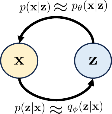
Figure 1: In a variational autoencoder, the variables $\mathbf{x}$ and $\mathbf{z}$ are connected by the conditional distributions $p(\mathbf{x}|\mathbf{z})$ and $p(\mathbf{z}|\mathbf{x})$. To make things work, we introduce two proxy distributions $p_{\boldsymbol{\theta}}(\mathbf{x}|\mathbf{z})$ and $q_{\boldsymbol{\phi}}(\mathbf{z}|\mathbf{x})$, respectively.

Example. It’s time to consider another trivial example. Suppose that we have a random variable $\mathbf{x}$ and a latent variable $\mathbf{z}$ such that $\displaystyle\mathbf{x}$ $\displaystyle\sim\mathcal{N}(\mathbf{x}\,|\,\mu,\sigma^{2}),$ $\displaystyle\mathbf{z}$ $\displaystyle\sim\mathcal{N}(\mathbf{z}\,|\,0,1).$ Our goal is to construct a VAE. (What?! This problem has a trivial solution where $\mathbf{z}=(\mathbf{x}-\mu)/\sigma$ and $\mathbf{x}=\boldsymbol{\mu}+\sigma\mathbf{z}$. You are absolutely correct. But please follow our derivation to see if the VAE framework makes sense.) By constructing a VAE, we mean that we want to build two mappings “encode” and “decode”. For simplicity, let’s assume that both mappings are affine transformations: $\displaystyle\mathbf{z}$ $\displaystyle=\text{encode}(\mathbf{x})=a\mathbf{x}+b,\qquad\text{so that}\quad\boldsymbol{\phi}=[a,b],$ $\displaystyle\mathbf{x}$ $\displaystyle=\text{decode}(\mathbf{z})=c\mathbf{z}+d,\qquad\text{so that}\quad\boldsymbol{\theta}=[c,d].$ We are too lazy to find out the joint distribution $p(\mathbf{x},\mathbf{z})$, nor the conditional distributions $p(\mathbf{x}|\mathbf{z})$ and $p(\mathbf{z}|\mathbf{x})$. But we can construct the proxy distributions $q_{\boldsymbol{\phi}}(\mathbf{z}|\mathbf{x})$ and $p_{\boldsymbol{\theta}}(\mathbf{x}|\mathbf{z})$. Since we have the freedom to choose what $q_{\boldsymbol{\phi}}$ and $p_{\boldsymbol{\theta}}$ should look like, how about we consider the following two Gaussians $\displaystyle q_{\boldsymbol{\phi}}(\mathbf{z}|\mathbf{x})$ $\displaystyle=\mathcal{N}(\mathbf{z}\;|\;a\mathbf{x}+b,1),$ $\displaystyle p_{\boldsymbol{\theta}}(\mathbf{x}|\mathbf{z})$ $\displaystyle=\mathcal{N}(\mathbf{x}\;|\;c\mathbf{z}+d,c).$ The choice of these two Gaussians is not mysterious. For $q_{\boldsymbol{\phi}}(\mathbf{z}|\mathbf{x})$: if we are given $\mathbf{x}$, of course we want the encoder to encode the distribution according to the structure we have chosen. Since the encoder structure is $a\mathbf{x}+b$, the natural choice for $q_{\boldsymbol{\phi}}(\mathbf{z}|\mathbf{x})$ is to have the mean $a\mathbf{x}+b$. The variance is chosen as 1 because we know that the encoded sample $\mathbf{z}$ should be unit-variance. Similarly, for $p_{\boldsymbol{\theta}}(\mathbf{x}|\mathbf{z})$: if we are given $\mathbf{z}$, the decoder must take the form of $c\mathbf{z}+d$ because this is how we setup the decoder. The variance is $c$ which is a parameter we need to figure out. We will pause for a moment before continuing this example. We want to introduce a mathematical tool.

1.2 Evidence Lower Bound

How do we use these two proxy distributions to achieve our goal of determining the encoder and the decoder? If we treat $\boldsymbol{\phi}$ and $\boldsymbol{\theta}$ as optimization variables, then we need an objective function (or the loss function) so that we can optimize $\boldsymbol{\phi}$ and $\boldsymbol{\theta}$ through training samples. To this end, we need to set up a loss function in terms of $\boldsymbol{\phi}$ and $\boldsymbol{\theta}$. The loss function we use here is called the Evidence Lower BOund (ELBO) [1]: $$\text{ELBO}(\mathbf{x})\overset{\text{def}}{=}\mathbb{E}_{q_{\phi}(\mathbf{z}|\mathbf{x})}\left[\log\frac{p(\mathbf{x},\mathbf{z})}{q_{\boldsymbol{\phi}}(\mathbf{z}|\mathbf{x})}\right].$$ (2) You are certainly puzzled how on the Earth people can come up with this loss function!? Let’s see what ELBO means and how it is derived.

In a nutshell, ELBO is a lower bound for the prior distribution $\log p(\mathbf{x})$ because we can show that

$$\log p(\mathbf{x})=\text{some magical steps} =\mathbb{E}_{q_{\phi}(\mathbf{z}|\mathbf{x})}\left[\log\frac{p(\mathbf{x},\mathbf{z})}{q_{\boldsymbol{\phi}}(\mathbf{z}|\mathbf{x})}\right]+\mathbb{D}_{\text{KL}}(q_{\boldsymbol{\phi}}(\mathbf{z}|\mathbf{x})\|p(\mathbf{z}|\mathbf{x}))$$ (3)

$$\geq\mathbb{E}_{q_{\phi}(\mathbf{z}|\mathbf{x})}\left[\log\frac{p(\mathbf{x},\mathbf{z})}{q_{\boldsymbol{\phi}}(\mathbf{z}|\mathbf{x})}\right]$$

$$\overset{\text{def}}{=}\text{ELBO}(\mathbf{x}),$$

where the inequality follows from the fact that the KL divergence is always non-negative. Therefore, ELBO is a valid lower bound for $\log p(\mathbf{x})$. Since we never have access to $\log p(\mathbf{x})$, if we somehow have access to ELBO and if ELBO is a good lower bound, then we can effectively maximize ELBO to achieve the goal of maximizing $\log p(\mathbf{x})$ which is the gold standard. Now, the question is how good the lower bound is. As you can see from the equation and also Figure 2, the inequality will become an equality when our proxy $q_{\boldsymbol{\phi}}(\mathbf{z}|\mathbf{x})$ can match the true distribution $p(\mathbf{z}|\mathbf{x})$ exactly. So, part of the game is to ensure $q_{\boldsymbol{\phi}}(\mathbf{z}|\mathbf{x})$ is close to $p(\mathbf{z}|\mathbf{x})$.

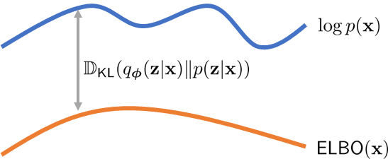
Figure 2: Visualization of $\log p(\mathbf{x})$ and ELBO. The gap between the two is determined by the KL divergence $\mathbb{D}_{\text{KL}}(q_{\boldsymbol{\phi}}(\mathbf{z}|\mathbf{x})\|p(\mathbf{z}|\mathbf{x}))$.

Proof of Eqn (3). The whole trick here is to use our magical proxy $q_{\boldsymbol{\phi}}(\mathbf{z}|\mathbf{x})$ to poke around $p(\mathbf{x})$ and derive the bound. $\displaystyle\log p(\mathbf{x})$ $\displaystyle=\log p(\mathbf{x})\times\underset{=1}{\underbrace{\int q_{\boldsymbol{\phi}}(\mathbf{z}|\mathbf{x})d\mathbf{z}}}$ multiply 1 $\displaystyle=\int\underset{\text{some constant wrt $\mathbf{z}$}}{\underbrace{\log p(\mathbf{x})}}\times\underset{\text{distribution in $\mathbf{z}$}}{\underbrace{q_{\boldsymbol{\phi}}(\mathbf{z}|\mathbf{x})}}d\mathbf{z}$ move $\log p(\mathbf{x})$ into integral $\displaystyle=\mathbb{E}_{q_{\boldsymbol{\phi}}(\mathbf{z}|\mathbf{x})}[\log p(\mathbf{x})],$ (4) where the last equality is an interesting fact that $\int a\times p_{Z}(z)dz=\mathbb{E}[a]$ for any random variable $Z$ and a scalar $a$. Of course, $\mathbb{E}[a]=a$. See, we have already got $\mathbb{E}_{q_{\boldsymbol{\phi}}(\mathbf{z}|\mathbf{x})}[\cdot]$. Just a few more steps. Let’s use Bayes theorem which states that $p(\mathbf{x},\mathbf{z})=p(\mathbf{z}|\mathbf{x})p(\mathbf{x})$: $\displaystyle\mathbb{E}_{q_{\boldsymbol{\phi}}(\mathbf{z}|\mathbf{x})}[\log p(\mathbf{x})]$ $\displaystyle=\mathbb{E}_{q_{\boldsymbol{\phi}}(\mathbf{z}|\mathbf{x})}\left[\log\frac{p(\mathbf{x},\mathbf{z})}{p(\mathbf{z}|\mathbf{x})}\right]$ Bayes Theorem $\displaystyle=\mathbb{E}_{q_{\boldsymbol{\phi}}(\mathbf{z}|\mathbf{x})}\left[\log\frac{p(\mathbf{x},\mathbf{z})}{p(\mathbf{z}|\mathbf{x})}\times{\color[rgb]{0,0,1}\frac{q_{\boldsymbol{\phi}}(\mathbf{z}|\mathbf{x})}{q_{\boldsymbol{\phi}}(\mathbf{z}|\mathbf{x})}}\right]$ Multiply and divide $q_{\boldsymbol{\phi}}(\mathbf{z}|\mathbf{x})$ $\displaystyle=\underset{\text{ELBO}}{\underbrace{\mathbb{E}_{q_{\boldsymbol{\phi}}(\mathbf{z}|\mathbf{x})}\left[\log\frac{p(\mathbf{x},\mathbf{z})}{{\color[rgb]{0,0,1}q_{\boldsymbol{\phi}}(\mathbf{z}|\mathbf{x})}}\right]}}+\underset{\mathbb{D}_{\text{KL}}(q_{\boldsymbol{\phi}}(\mathbf{z}|\mathbf{x})\|p(\mathbf{z}|\mathbf{x}))}{\underbrace{\mathbb{E}_{q_{\boldsymbol{\phi}}(\mathbf{z}|\mathbf{x})}\left[\log\frac{{\color[rgb]{0,0,1}q_{\boldsymbol{\phi}}(\mathbf{z}|\mathbf{x})}}{p(\mathbf{z}|\mathbf{x})}\right]}},$ (5) where we recognize that the first term is exactly ELBO, whereas the second term is exactly the KL divergence. Comparing Eqn (5) with Eqn (3), we know that life is good.

We now have ELBO. But this ELBO is still not too useful because it involves $p(\mathbf{x},\mathbf{z})$, something we have no access to. So, we need to do a little more things. Let’s take a closer look at ELBO

$$\text{ELBO}(\mathbf{x}) \overset{\text{def}}{=}\mathbb{E}_{q_{\boldsymbol{\phi}}(\mathbf{z}|\mathbf{x})}\left[\log\frac{p(\mathbf{x},\mathbf{z})}{q_{\boldsymbol{\phi}}(\mathbf{z}|\mathbf{x})}\right]$$ definition

$$=\mathbb{E}_{q_{\boldsymbol{\phi}}(\mathbf{z}|\mathbf{x})}\left[\log\frac{{\color[rgb]{0,0,1}p(\mathbf{x}|\mathbf{z})p(\mathbf{z})}}{q_{\boldsymbol{\phi}}(\mathbf{z}|\mathbf{x})}\right] \qquad p(\mathbf{x},\mathbf{z})=p(\mathbf{x}|\mathbf{z})p(\mathbf{z})$$

$$=\mathbb{E}_{q_{\boldsymbol{\phi}}(\mathbf{z}|\mathbf{x})}\left[\log p(\mathbf{x}|\mathbf{z})\right]+\mathbb{E}_{q_{\boldsymbol{\phi}}(\mathbf{z}|\mathbf{x})}\left[\log\frac{p(\mathbf{z})}{q_{\boldsymbol{\phi}}(\mathbf{z}|\mathbf{x})}\right]$$ split expectation

$$=\mathbb{E}_{q_{\boldsymbol{\phi}}(\mathbf{z}|\mathbf{x})}\left[\log{\color[rgb]{0,0,1}p_{\boldsymbol{\theta}}(\mathbf{x}|\mathbf{z})}\right]-\mathbb{D}_{\text{KL}}(q_{\boldsymbol{\phi}}(\mathbf{z}|\mathbf{x})\|p(\mathbf{z})),$$ definition of KL

where we secretly replaced the inaccessible $p(\mathbf{x}|\mathbf{z})$ by its proxy $p_{\boldsymbol{\theta}}(\mathbf{x}|\mathbf{z})$. This is a beautiful result. We just showed something very easy to understand. $$\text{ELBO}(\mathbf{x})=\underset{\text{how good your decoder is}}{\underbrace{\mathbb{E}_{q_{\phi}(\mathbf{z}|\mathbf{x})}[\log\overset{\text{a Gaussian}}{\overbrace{p_{\boldsymbol{\theta}}(\mathbf{x}|\mathbf{z})}}]}}\qquad\qquad-\qquad\qquad\underset{\text{how good your encoder is}}{\underbrace{\mathbb{D}_{\text{KL}}\Big{(}\overset{\text{a Gaussian}}{\overbrace{q_{\phi}(\mathbf{z}|\mathbf{x})}}\,\|\,\overset{\text{a Gaussian}}{\overbrace{p(\mathbf{z})}}\Big{)}}}.$$ (6) There are two terms in Eqn (6):

• Reconstruction. The first term is about the decoder. We want the decoder to produce a good image $\mathbf{x}$ if we feed a latent $\mathbf{z}$ into the decoder (of course!!). So, we want to maximize $\log p_{\boldsymbol{\theta}}(\mathbf{x}|\mathbf{z})$. It is similar to maximum likelihood where we want to find the model parameter to maximize the likelihood of observing the image. The expectation here is taken with respect to the samples $\mathbf{z}$ (conditioned on $\mathbf{x}$). This shouldn’t be a surprise because the samples $\mathbf{z}$ are used to assess the quality of the decoder. It cannot be an arbitrary noise vector but a meaningful latent vector. So, $\mathbf{z}$ needs to be sampled from $q_{\phi}(\mathbf{z}|\mathbf{x})$.

• Prior Matching. The second term is the KL divergence for the encoder. We want the encoder to turn $\mathbf{x}$ into a latent vector $\mathbf{z}$ such that the latent vector will follow our choice of (lazy) distribution $\mathcal{N}(0,\mathbf{I})$. To be slightly more general, we write $p(\mathbf{z})$ as the target distribution. Because KL is a distance (which increases when the two distributions become more dissimilar), we need to put a negative sign in front so that it increases when the two distributions become more similar.

Example. Let’s continue our trivial Gaussian example. We know from our previous derivation that $\displaystyle q_{\boldsymbol{\phi}}(\mathbf{z}|\mathbf{x})$ $\displaystyle=\mathcal{N}(\mathbf{z}\;|\;a\mathbf{x}+b,1),$ $\displaystyle p_{\boldsymbol{\theta}}(\mathbf{x}|\mathbf{z})$ $\displaystyle=\mathcal{N}(\mathbf{x}\;|\;c\mathbf{z}+d,c).$ To determine $\boldsymbol{\theta}$ and $\boldsymbol{\phi}$, we need to minimize the prior matching error and maximize the reconstruction term. For the prior matching, we know that $\displaystyle\mathbb{D}_{\text{KL}}(q_{\boldsymbol{\phi}}(\mathbf{z}|\mathbf{x})\|p(\mathbf{z}))=\mathbb{D}_{\text{KL}}\left(\mathcal{N}(\mathbf{z}\;|\;a\mathbf{x}+b,1)\;\|\;\mathcal{N}(\mathbf{z}\;|\;0,1)\right).$ Since $\mathbb{E}[\mathbf{x}]=\mu$ and $\mathrm{Var}[\mathbf{x}]=\sigma^{2}$, the KL-divergence is minimized when $a=\frac{1}{\sigma}$ and $b=-\frac{\mu}{\sigma}$ so that $a\mathbf{x}+b=\frac{\mathbf{x}-\mu}{\sigma}$. It then follows that $\mathbb{E}[a\mathbf{x}+b]=0$, and $\mathrm{Var}[a\mathbf{x}+b]=1$. For the reconstruction term, we know that $\displaystyle\mathbb{E}_{q_{\boldsymbol{\phi}}(\mathbf{z}|\mathbf{x})}[\log p_{\boldsymbol{\theta}}(\mathbf{x}|\mathbf{z})]=\mathbb{E}_{q_{\boldsymbol{\phi}}(\mathbf{z}|\mathbf{x})}\left[-\frac{(c\mathbf{z}+d-\mu)^{2}}{2c^{2}}\right].$ Since $\mathbb{E}[\mathbf{z}]=0$ and $\mathrm{Var}[\mathbf{z}]=1$, it follows that the term is maximized when $c=\sigma$ and $d=\mu$. To conclude, the encoder and decoder parameters are $\displaystyle\mathbf{z}$ $\displaystyle=\text{encode}(\mathbf{x})=\frac{\mathbf{x}-\mu}{\sigma},$ $\displaystyle\mathbf{x}$ $\displaystyle=\text{decode}(\mathbf{z})=\sigma\mathbf{z}+\mu,$ which is fairly easy to understand.

The reconstruction term and the prior matching terms are illustrated in Figure 3. In both cases, and during training, we assume that we have access to both $\mathbf{z}$ and $\mathbf{x}$, where $\mathbf{z}$ needs to be sampled from $q_{\boldsymbol{\phi}}(\mathbf{z}|\mathbf{x})$. Then for reconstruction, we estimate $\boldsymbol{\theta}$ to maximize $p_{\boldsymbol{\theta}}(\mathbf{x}|\mathbf{z})$. For prior matching, we find $\boldsymbol{\phi}$ to minimize the KL divergence. The optimization can be challenging, because if you update $\boldsymbol{\phi}$, the distribution $q_{\boldsymbol{\phi}}(\mathbf{z}|\mathbf{x})$ will change.

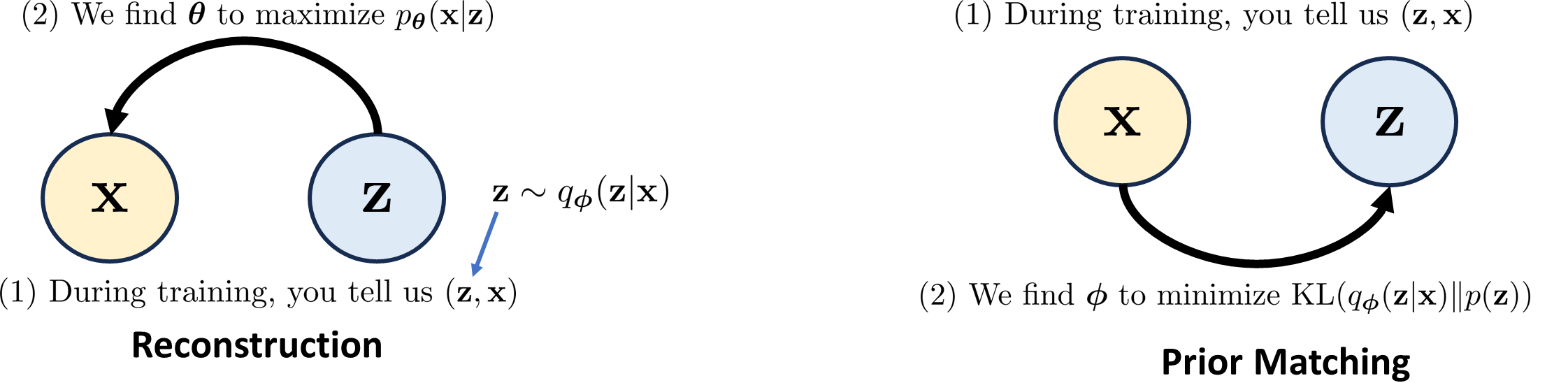
Figure 3: Interpreting the reconstruction term and the prior matching term in ELBO for a variational autoencoder.

1.3 Training VAE

Now that we understand the meaning of ELBO, we can discuss how to train the VAE. To train a VAE, we need the ground truth pairs $(\mathbf{x},\mathbf{z})$. We know how to get $\mathbf{x}$; it is just the image from a dataset. But correspondingly what should $\mathbf{z}$ be?

Let’s talk about the encoder. We know that $\mathbf{z}$ is generated from the distribution $q_{\boldsymbol{\phi}}(\mathbf{z}|\mathbf{x})$. We also know that $q_{\boldsymbol{\phi}}(\mathbf{z}|\mathbf{x})$ is a Gaussian. Assume that this Gaussian has a mean $\boldsymbol{\mu}$ and a covariance matrix $\sigma^{2}\mathbf{I}$ (Ha! Our laziness again! We do not use a general covariance matrix but assume an equal variance).

The tricky part is how to determine $\boldsymbol{\mu}$ and $\sigma^{2}$ from the input image $\mathbf{x}$. Okay, if you run out of clue, do not worry. Welcome to the Dark Side of the Force. We construct a deep neural network(s) such that

$$\boldsymbol{\mu} =\underset{\text{neural network}}{\underbrace{\boldsymbol{\mu}_{\boldsymbol{\phi}}}}(\mathbf{x})$$

$$\sigma^{2} =\underset{\text{neural network}}{\underbrace{\sigma_{\boldsymbol{\phi}}^{2}}}(\mathbf{x}),$$

Therefore, the samples $\mathbf{z}^{(\ell)}$ (where $\ell$ denotes the $\ell$-th training sample in the training set) can be sampled from the Gaussian distribution

$$\mathbf{z}^{(\ell)}\sim\underset{q_{\boldsymbol{\phi}}(\mathbf{z}|\mathbf{x}^{(\ell)})}{\underbrace{\mathcal{N}(\mathbf{z}\;|\;\boldsymbol{\mu}_{\boldsymbol{\phi}}(\mathbf{x}^{(\ell)}),\sigma_{\boldsymbol{\phi}}^{2}(\mathbf{x}^{(\ell)})\mathbf{I})}},\qquad\text{where $\boldsymbol{\mu}_{\boldsymbol{\phi}},\sigma_{\boldsymbol{\phi}}^{2}$ are functions of $\mathbf{x}$.}$$ (7)

The idea is summarized in Figure 4 where we use a neural network to estimate the Gaussian parameters, and from the Gaussian we draw samples. Note that $\boldsymbol{\mu}_{\boldsymbol{\phi}}(\mathbf{x}^{(\ell)})$ and $\sigma_{\boldsymbol{\phi}}^{2}(\mathbf{x}^{(\ell)})$ are functions of $\mathbf{x}^{(\ell)}$. Thus, for a different $\mathbf{x}^{(\ell)}$ we will have a different Gaussian.

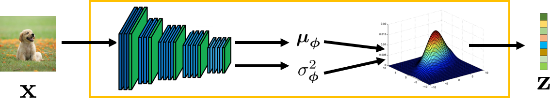
Figure 4: Implementation of a VAE encoder. We use a neural network to take the image $\mathbf{x}$ and estimate the mean $\boldsymbol{\mu}_{\boldsymbol{\phi}}$ and variance $\sigma^{2}_{\boldsymbol{\phi}}$ of the Gaussian distribution.

Remark. For any high-dimensional Gaussian $\mathbf{x}\sim\mathcal{N}(\mathbf{x}|\boldsymbol{\mu},\boldsymbol{\Sigma})$, the sampling process can be done via the transformation of white noise $$\mathbf{x}=\boldsymbol{\mu}+\boldsymbol{\Sigma}^{\frac{1}{2}}\mathbf{w},$$ (8) where $\mathbf{w}\sim\mathcal{N}(0,\mathbf{I})$. The half matrix $\boldsymbol{\Sigma}^{\frac{1}{2}}$ can be obtained through eigen-decomposition or Cholesky factorization. For diagonal matrices $\boldsymbol{\Sigma}=\sigma^{2}\mathbf{I}$, the above reduces to $$\mathbf{x}=\boldsymbol{\mu}+\sigma\mathbf{w},\qquad\text{where}\;\mathbf{w}\sim\mathcal{N}(0,\mathbf{I}).$$ (9)

Let’s talk about the decoder. The decoder is implemented through a neural network. For notation simplicity, let’s define it as $\text{decode}_{\boldsymbol{\theta}}$ where $\boldsymbol{\theta}$ denotes the network parameters. The job of the decoder network is to take a latent variable $\mathbf{z}$ and generates an image $\widehat{\mathbf{x}}$:

$$\widehat{\mathbf{x}}=\text{decode}_{\boldsymbol{\theta}}(\mathbf{z}).$$ (10)

Now let’s make one more (crazy) assumption that the error between the decoded image $\widehat{\mathbf{x}}$ and the ground truth image $\mathbf{x}$ is Gaussian. (Wait, Gaussian again?!) We assume that

$$(\widehat{\mathbf{x}}-\mathbf{x})\sim\mathcal{N}(0,\sigma_{\text{dec}}^{2}),\qquad\text{for some $\sigma_{\text{dec}}^{2}$.}$$

Then, it follows that the distribution $p_{\boldsymbol{\theta}}(\mathbf{x}|\mathbf{z})$ is

$$\log p_{\boldsymbol{\theta}}(\mathbf{x}|\mathbf{z}) =\log\mathcal{N}(\mathbf{x}\,|\,\text{decode}_{\boldsymbol{\theta}}(\mathbf{z}),\sigma_{\text{dec}}^{2}\mathbf{I})$$

$$=\log\frac{1}{\sqrt{(2\pi\sigma_{\text{dec}}^{2})^{D}}}\exp\left\{-\frac{\|\mathbf{x}-\text{decode}_{\boldsymbol{\theta}}(\mathbf{z})\|^{2}}{2\sigma_{\text{dec}}^{2}}\right\}$$

$$=-\frac{\|\mathbf{x}-\text{decode}_{\boldsymbol{\theta}}(\mathbf{z})\|^{2}}{2\sigma_{\text{dec}}^{2}}\;\;-\;\;\underset{\text{you can ignore this term}}{\underbrace{\log\sqrt{(2\pi\sigma_{\text{dec}}^{2})^{D}}}},$$ (11)

where $D$ is the dimension of $\mathbf{x}$. This equation says that the maximization of the likelihood term in ELBO is literally just the $\ell_{2}$ loss between the decoded image and ground truth. The idea is shown in Figure 5.

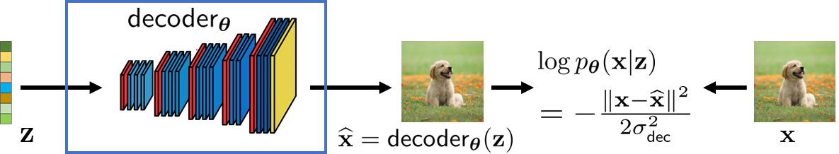
Figure 5: Implementation of a VAE decoder. We use a neural network to take the latent vector $\mathbf{z}$ and generate an image $\widehat{\mathbf{x}}$. The log likelihood will give us a quadratic equation if we assume a Gaussian distribution.

1.4 Loss Function

Once you understand the structure of the encoder and the decoder, the loss function is easy to understand. We approximate the expectation by Monte-Carlo simulation:

$$\mathbb{E}_{q_{\boldsymbol{\phi}}(\mathbf{z}|\mathbf{x})}[\log p_{\boldsymbol{\theta}}(\mathbf{x}|\mathbf{z})]\approx\frac{1}{L}\sum_{\ell=1}^{L}\log p_{\boldsymbol{\theta}}(\mathbf{x}^{\ell}|\mathbf{z}^{(\ell)}),\qquad\mathbf{z}^{(\ell)}\sim q_{\boldsymbol{\phi}}(\mathbf{z}|\mathbf{x}^{(\ell)}),$$

where $\mathbf{x}^{(\ell)}$ is the $\ell$-th sample in the training set, and $\mathbf{z}^{(\ell)}$ is sampled from $\mathbf{z}^{(\ell)}\sim q_{\boldsymbol{\phi}}(\mathbf{z}|\mathbf{x}^{(\ell)})$. The distribution $q_{\boldsymbol{\theta}}$ is $q_{\boldsymbol{\phi}}(\mathbf{z}|\mathbf{x}^{(\ell)})=\mathcal{N}(\mathbf{z}|\boldsymbol{\mu}_{\boldsymbol{\phi}}(\mathbf{x}^{(\ell)}),\sigma^{2}_{\boldsymbol{\phi}}(\mathbf{x}^{(\ell)})\mathbf{I})$.

Training loss of VAE: $$\mathop{\underset{\boldsymbol{\phi},\boldsymbol{\theta}}{\mbox{argmax}}}\left\{\frac{1}{L}\sum_{\ell=1}^{L}\log p_{\boldsymbol{\theta}}(\mathbf{x}^{(\ell)}|\mathbf{z}^{(\ell)})-\mathbb{D}_{\text{KL}}(q_{\boldsymbol{\phi}}(\mathbf{z}|\mathbf{x}^{(\ell)})\|p(\mathbf{z}))\right\},$$ (12) where $\{\mathbf{x}^{(\ell)}\}_{\ell=1}^{L}$ are the ground truth images in the training dataset, and $\mathbf{z}^{(\ell)}$ is sampled from Eqn (7).

The $\mathbf{z}$ in the KL divergence term does not depend on $\ell$ because we are measuring the KL divergence between two distributions. The variable $\mathbf{z}$ here is a dummy.

One last thing we need to clarify is the KL divergence. Since $q_{\boldsymbol{\phi}}(\mathbf{z}|\mathbf{x}^{(\ell)})=\mathcal{N}(\mathbf{z}|\boldsymbol{\mu}_{\boldsymbol{\phi}}(\mathbf{x}^{(\ell)}),\sigma^{2}_{\boldsymbol{\phi}}(\mathbf{x}^{(\ell)})\mathbf{I})$ and $p(\mathbf{z})=\mathcal{N}(0,\mathbf{I})$, we are essentially coming two Gaussian distributions. If you go to Wikipedia, you can see that the KL divergence for two $d$-dimensional Gaussian distributions $\mathcal{N}(\boldsymbol{\mu}_{0},\boldsymbol{\Sigma}_{0})$ and $\mathcal{N}(\boldsymbol{\mu}_{1},\boldsymbol{\Sigma}_{1})$ is

$$\mathbb{D}_{\text{KL}}(\mathcal{N}(\boldsymbol{\mu}_{0},\boldsymbol{\Sigma}_{0}),\mathcal{N}(\boldsymbol{\mu}_{1},\boldsymbol{\Sigma}_{1}))=\frac{1}{2}\left(\text{Tr}(\boldsymbol{\Sigma}_{1}^{-1}\boldsymbol{\Sigma}_{0})-d+(\boldsymbol{\mu}_{1}-\boldsymbol{\mu}_{0})^{T}\boldsymbol{\Sigma}_{1}^{-1}(\boldsymbol{\mu}_{1}-\boldsymbol{\mu}_{0})+\log\frac{\text{det}\boldsymbol{\Sigma}_{1}}{\text{det}\boldsymbol{\Sigma}_{0}}\right).$$ (13)

Substituting our distributions by considering $\boldsymbol{\mu}_{0}=\boldsymbol{\mu}_{\boldsymbol{\phi}}(\mathbf{x}^{(\ell)})$, $\boldsymbol{\Sigma}_{0}=\sigma^{2}_{\boldsymbol{\phi}}(\mathbf{x}^{(\ell)})\mathbf{I}$, $\boldsymbol{\mu}_{1}=0$, $\boldsymbol{\Sigma}_{1}=\mathbf{I}$, we can show that the KL divergence has an analytic expression

$$\mathbb{D}_{\text{KL}}(q_{\boldsymbol{\phi}}(\mathbf{z}|\mathbf{x}^{(\ell)})\;\|\;p(\mathbf{z}))=\frac{1}{2}\left((\sigma_{\boldsymbol{\phi}}^{2}(\mathbf{x}^{(\ell)}))^{d}+\boldsymbol{\mu}_{\boldsymbol{\phi}}(\mathbf{x}^{(\ell)})^{T}\boldsymbol{\mu}_{\boldsymbol{\phi}}(\mathbf{x}^{(\ell)})-d\log(\sigma_{\boldsymbol{\phi}}^{2}(\mathbf{x}^{(\ell)}))\right),$$ (14)

where $d$ is the dimension of the vector $\mathbf{z}$. Therefore, the overall loss function Eqn (12) is differentiable. So, we can train the encoder and the decoder end-to-end by backpropagating the gradients.

1.5 Inference with VAE

For inference, we can simply throw a latent vector $\mathbf{z}$ (which is sampled from $p(\mathbf{z})=\mathcal{N}(0,\mathbf{I})$) into the decoder $\text{decode}_{\boldsymbol{\theta}}$ and get an image $\mathbf{x}$. That’s it; see Figure 6.

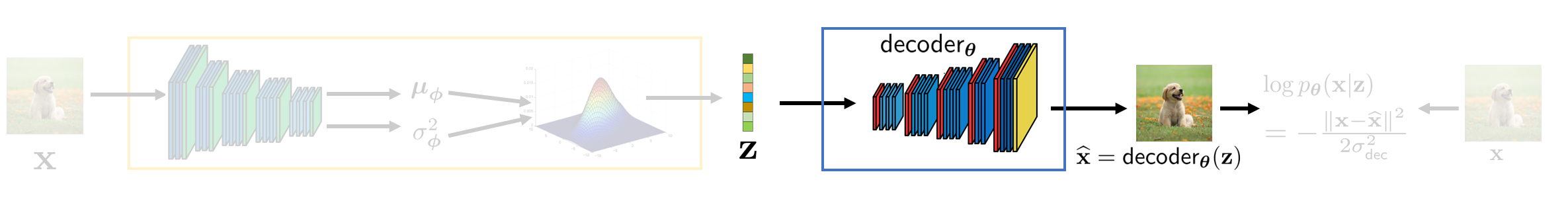
Figure 6: Using VAE to generate image is as simple as sending a latent noise code $\mathbf{z}$ through the decoder.

Congratulations! We are done. This is all about VAE.

If you would like to read more, we highly recommend the tutorial by Kingma and Welling [1]. A shorter tutorial can be found at [2]. If you type VAE tutorial PyTorch in Google, you will be able to find hundreds if not thousands programming tutorials and videos.

2 Denoising Diffusion Probabilistic Model (DDPM)

In this section, we will discuss the DDPM by Ho et al. [4]. If you are confused by the thousands of tutorials online, rest assured that DDPM is not that complicated. All you need to understand is the following summary:

Diffusion models are incremental updates where the assembly of the whole gives us the encoder-decoder structure. The transition from one state to another is realized by a denoiser.

Why increment? It’s like turning the direction of a giant ship. You need to turn the ship slowly towards your desired direction or otherwise you will lose control. The same principle applies to your life, your company HR, your university administration, your spouse, your children, and anything around your life. “Bend one inch at a time!” (Credit: Sergio Goma who made this comment at Electronic Imaging 2023.)

The structure of the diffusion model is shown below. It is called the variational diffusion model [5]. The variational diffusion model has a sequence of states $\mathbf{x}_{0},\mathbf{x}_{1},\ldots,\mathbf{x}_{T}$:

• $\mathbf{x}_{0}$: It is the original image, which is the same as $\mathbf{x}$ in VAE.

• $\mathbf{x}_{T}$: It is the latent variable, which is the same as $\mathbf{z}$ in VAE. Since we are all lazy, we want $\mathbf{x}_{T}\sim\mathcal{N}(0,\mathbf{I})$.

• $\mathbf{x}_{1},\ldots,\mathbf{x}_{T-1}$: They are the intermediate states. They are also the latent variables, but they are not white Gaussian.

The structure of the variational diffusion model is shown in Figure 7. The forward and the reverse paths are analogous to the paths of a single-step variational autoencoder. The difference is that the encoders and decoders have identical input-output dimensions. The assembly of all the forward building blocks will give us the encoder, and the assembly of all the reverse building blocks will give us the decoder.

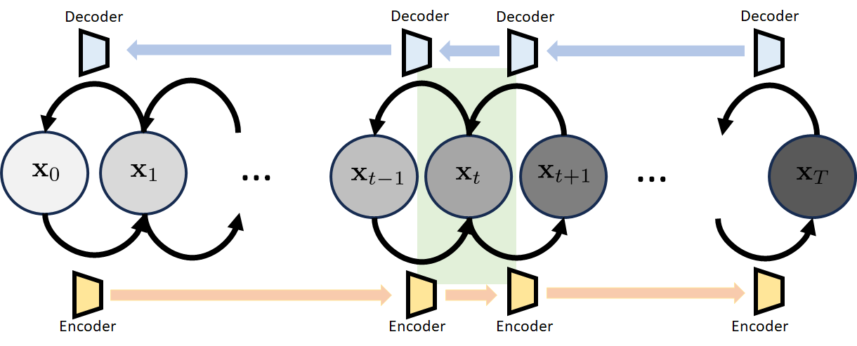
Figure 7: Variational diffusion model. In this model, the input image is $\mathbf{x}_{0}$ and the white noise is $\mathbf{x}_{T}$. The intermediate variables (or states) $\mathbf{x}_{1},\ldots,\mathbf{x}_{T-1}$ are latent variables. The transition from $\mathbf{x}_{t-1}$ to $\mathbf{x}_{t}$ is analogous to the forward step (encoder) in VAE, whereas the transition from $\mathbf{x}_{t}$ to $\mathbf{x}_{t-1}$ is analogous to the reverse step (decoder) in VAE. Note, however, that the input dimension and the output dimension of the encoders/decoders here are identical.

2.1 Building Blocks

Transition Block The $t$-th transition block consists of three states $\mathbf{x}_{t-1}$, $\mathbf{x}_{t}$, and $\mathbf{x}_{t+1}$. There are two possible paths to get to state $\mathbf{x}_{t}$, as illustrated in Figure 8.

• The forward transition that goes from $\mathbf{x}_{t-1}$ to $\mathbf{x}_{t}$. The associated transition distribution is $p(\mathbf{x}_{t}|\mathbf{x}_{t-1})$. In plain words, if you tell us $\mathbf{x}_{t-1}$, we can tell you $\mathbf{x}_{t}$ according to $p(\mathbf{x}_{t}|\mathbf{x}_{t-1})$. However, just like a VAE, the transition distribution $p(\mathbf{x}_{t}|\mathbf{x}_{t-1})$ is never accessible. But this is okay. Lazy people like us will just approximate it by a Gaussian $q_{\boldsymbol{\phi}}(\mathbf{x}_{t}|\mathbf{x}_{t-1})$. We will discuss the exact form $q_{\boldsymbol{\phi}}$ later, but it is just some Gaussian.

• The reverse transition goes from $\mathbf{x}_{t+1}$ to $\mathbf{x}_{t}$. Again, we never know $p(\mathbf{x}_{t+1}|\mathbf{x}_{t})$ but that’s okay. We just use another Gaussian $p_{\boldsymbol{\theta}}(\mathbf{x}_{t+1}|\mathbf{x}_{t})$ to approximate the true distribution, but its mean needs to be estimated by a neural network.

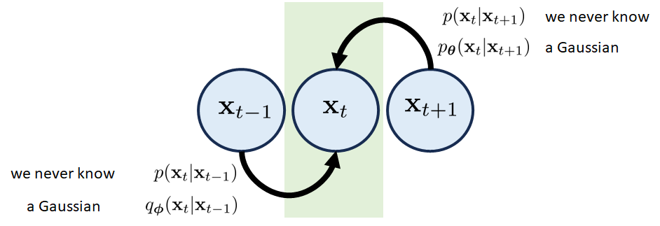
Figure 8: The transition block of a variational diffusion model consists of three nodes. The transition distributions $p(\mathbf{x}_{t}|\mathbf{x}_{t+1})$ and $p(\mathbf{x}_{t}|\mathbf{x}_{t-1})$ are not accessible, but we can approximate them by Gaussians.

Initial Block The initial block of the variational diffusion model focuses on the state $\mathbf{x}_{0}$. Since all problems we study starts at $\mathbf{x}_{0}$, there is only the reverse transition from $\mathbf{x}_{1}$ to $\mathbf{x}_{0}$, and nothing that goes from $\mathbf{x}_{-1}$ to $\mathbf{x}_{0}$. Therefore, we only need to worry about $p(\mathbf{x}_{0}|\mathbf{x}_{1})$. But since $p(\mathbf{x}_{0}|\mathbf{x}_{1})$ is never accessible, we approximate it by a Gaussian $p_{\boldsymbol{\theta}}(\mathbf{x}_{0}|\mathbf{x}_{1})$ where the mean is computed through a neural network. See Figure 9 for illustration.

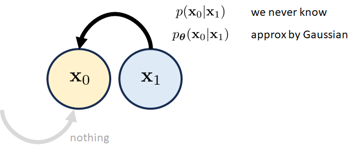
Figure 9: The initial block of a variational diffusion model focuses on the node $\mathbf{x}_{0}$. Since there is no state before time $t=0$, we only have a reverse transition from $\mathbf{x}_{1}$ to $\mathbf{x}_{0}$.

Final Block. The final block focuses on the state $\mathbf{x}_{T}$. Remember that $\mathbf{x}_{T}$ is supposed to be our final latent variable which is a white Gaussian noise vector. Because it is the final block, there is only a forward transition from $\mathbf{x}_{T-1}$ to $\mathbf{x}_{T}$, and nothing such as $\mathbf{x}_{T+1}$ to $\mathbf{x}_{T}$. The forward transition is approximated by $q_{\boldsymbol{\phi}}(\mathbf{x}_{T}|\mathbf{x}_{T-1})$, which is a Gaussian. See Figure 10 for illustration.

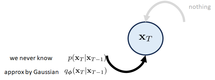
Figure 10: The final block of a variational diffusion model focuses on the node $\mathbf{x}_{T}$. Since there is no state after time $t=T$, we only have a forward transition from $\mathbf{x}_{T-1}$ to $\mathbf{x}_{T}$.

Understanding the Transition Distribution. Before we proceed further, we need to detour slightly to talk about the transition distribution $q_{\boldsymbol{\phi}}(\mathbf{x}_{t}|\mathbf{x}_{t-1})$. We know that it is Gaussian. But we still need to know its formal definition, and the origin of this definition.

Transition Distribution $q_{\boldsymbol{\phi}}(\mathbf{x}_{t}|\mathbf{x}_{t-1})$. In a denoising diffusion probabilistic model, the transition distribution $q_{\boldsymbol{\phi}}(\mathbf{x}_{t}|\mathbf{x}_{t-1})$ is defined as $$q_{\boldsymbol{\phi}}(\mathbf{x}_{t}|\mathbf{x}_{t-1})\overset{\text{def}}{=}\mathcal{N}(\mathbf{x}_{t}\,|\,\sqrt{\alpha_{t}}\mathbf{x}_{t-1},(1-\alpha_{t})\mathbf{I}).$$ (15)

In other words, the mean is $\sqrt{\alpha_{t}}\mathbf{x}_{t-1}$ and the variance is $1-\alpha_{t}$. The choice of the scaling factor $\sqrt{\alpha_{t}}$ is to make sure that the variance magnitude is preserved so that it will not explode and vanish after many iterations.

Example. Let’s consider a Gaussian mixture model $$\mathbf{x}_{0}\sim p_{0}(\mathbf{x})=\pi_{1}\mathcal{N}(\mathbf{x}|\mu_{1},\sigma_{1}^{2})+\pi_{2}\mathcal{N}(\mathbf{x}|\mu_{2},\sigma_{2}^{2}).$$ Given the transition probability, we know that $$\mathbf{x}_{t}=\sqrt{\alpha_{t}}\mathbf{x}_{t-1}+\sqrt{(1-\alpha_{t})}\boldsymbol{\epsilon},\qquad\text{where}\;\;\boldsymbol{\epsilon}\sim\mathcal{N}(0,\mathbf{I}).$$ For a mixture model, it is not difficult to show that the probability distribution of $\mathbf{x}_{t}$ can be calculated recursively via the algorithm for $t=1,2,\ldots,T$: $\displaystyle p_{t}(\mathbf{x})=$ $\displaystyle\pi_{1}\mathcal{N}(\mathbf{x}|\sqrt{\alpha_{t}}\mu_{1,t-1},\alpha_{t}\sigma_{1,t-1}^{2}+(1-\alpha_{t}))$ $\displaystyle+$ $\displaystyle\pi_{2}\mathcal{N}(\mathbf{x}|\sqrt{\alpha_{t}}\mu_{2,t-1},\alpha_{t}\sigma_{2,t-1}^{2}+(1-\alpha_{t})),$ (16) where $\mu_{1,t-1}$ is the mean at $t-1$, with $\mu_{1,0}=\mu_{1}$ being the initial mean. Similarly, $\sigma_{1,t-1}^{2}$ is the variance at $t-1$, with $\sigma_{1,0}^{2}=\sigma_{1}^{2}$ being the initial variance. In the figure below, we show the example where $\pi_{1}=0.3$, $\pi_{2}=0.7$, $\mu_{1}=-2$, $\mu_{2}=2$, $\sigma_{1}=0.2$, and $\sigma_{2}=1$. The rate is defined as $\alpha_{t}=0.97$ for all $t$. We plot the probability distribution function for different $t$.

Remark. For those who would like to understand how we derive the probability density of a mixture model in Eqn (16), we can show a simple derivation. Consider a mixture model $\displaystyle p(\mathbf{x})=\sum_{k=1}^{K}\pi_{k}\underset{p(\mathbf{x}|k)}{\underbrace{\mathcal{N}(\mathbf{x}|\mu_{k},\sigma_{k}^{2}\mathbf{I})}}.$ If we consider a new variable $\mathbf{y}=\sqrt{\alpha}\mathbf{x}+\sqrt{1-\alpha}\boldsymbol{\epsilon}$ where $\boldsymbol{\epsilon}\sim\mathcal{N}(0,\mathbf{I})$, then the distribution of $\mathbf{y}$ can be derived by using the law of total probability: $\displaystyle p(\mathbf{y})$ $\displaystyle=\sum_{k=1}^{K}p(\mathbf{y}|k)p(k)=\sum_{k=1}^{K}\pi_{k}p(\mathbf{y}|k).$ Since $\mathbf{y}|k$ is a linear combination of a Gaussian random variable $\mathbf{x}$ and another Gaussian random variable $\boldsymbol{\epsilon}$, the sum $\mathbf{y}$ will remain as a Gaussian. The mean is $\displaystyle\mathbb{E}[\mathbf{y}|k]$ $\displaystyle=\sqrt{\alpha}\mathbb{E}[\mathbf{x}|k]+\sqrt{1-\alpha}\mathbb{E}[\boldsymbol{\epsilon}]=\sqrt{\alpha}\mu_{k}$ $\displaystyle\mathrm{Var}[\mathbf{y}|k]$ $\displaystyle=\alpha\mathrm{Var}[\mathbf{x}|k]+(1-\alpha)\mathrm{Var}[\boldsymbol{\epsilon}]=\alpha\sigma_{k}^{2}+(1-\alpha).$ So, $p(\mathbf{y}|k)=\mathcal{N}(\mathbf{y}|\sqrt{\alpha}\mu_{k},\alpha\sigma_{k}^{2}+(1-\alpha))$. This completes the derivation.

2.2 The magical scalars $\sqrt{\alpha_{t}}$ and $1-\alpha_{t}$

You may wonder how the genie (the authors of the denoising diffusion) come up with the magical scalars $\sqrt{\alpha}_{t}$ and $(1-\alpha_{t})$ for the above transition probability. To demystify this, let’s begin with two unrelated scalars $a\in\mathbb{R}$ and $b\in\mathbb{R}$, and we define the transition distribution as

$$q_{\boldsymbol{\phi}}(\mathbf{x}_{t}|\mathbf{x}_{t-1})=\mathcal{N}(\mathbf{x}_{t}\,|\,a\mathbf{x}_{t-1},b^{2}\mathbf{I}).$$ (17)

Here is the rule of thumb: Why $\sqrt{\alpha_{t}}$ and $1-\alpha_{t}$? We want to choose $a$ and $b$ such that the distribution of $\mathbf{x}_{t}$ will become $\mathcal{N}(0,\mathbf{I})$ when $t$ is large enough. It turns out that the answer is $a=\sqrt{\alpha}$ and $b=\sqrt{1-\alpha}$. Proof. We want to show that $a=\sqrt{\alpha}$ and $b=\sqrt{1-\alpha}$. For the distribution shown in Eqn (17), the equivalent sampling step is: $$\mathbf{x}_{t}=a\mathbf{x}_{t-1}+b\boldsymbol{\epsilon}_{t-1},\qquad\text{where}\qquad\boldsymbol{\epsilon}_{t-1}\sim\mathcal{N}(0,\mathbf{I}).$$ (18) Think about this: if there is a random variable $X\sim\mathcal{N}(\mu,\sigma^{2})$, drawing $X$ from this Gaussian can be equivalently achieved by defining $X=\mu+\sigma\eta$ where $\eta\sim\mathcal{N}(0,1)$. We can carry on the recursion to show that $\displaystyle\mathbf{x}_{t}$ $\displaystyle=a\mathbf{x}_{t-1}+b\boldsymbol{\epsilon}_{t-1}$ $\displaystyle=a(a\mathbf{x}_{t-2}+b\boldsymbol{\epsilon}_{t-2})+b\boldsymbol{\epsilon}_{t-1}$ $\displaystyle\qquad(\text{substitute }\mathbf{x}_{t-1}=a\mathbf{x}_{t-2}+b\boldsymbol{\epsilon}_{t-2})$ $\displaystyle=a^{2}\mathbf{x}_{t-2}+ab\boldsymbol{\epsilon}_{t-2}+b\boldsymbol{\epsilon}_{t-1}$ $\displaystyle\qquad(\text{regroup terms })$ $\displaystyle=\vdots$ $\displaystyle=a^{t}\mathbf{x}_{0}+b\underset{\overset{\text{def}}{=}\mathbf{w}_{t}}{\underbrace{\left[\boldsymbol{\epsilon}_{t-1}+a\boldsymbol{\epsilon}_{t-2}+a^{2}\boldsymbol{\epsilon}_{t-3}+\ldots+a^{t-1}\boldsymbol{\epsilon}_{0}\right]}}.$ (19) The finite sum above is a sum of independent Gaussian random variables. The mean vector $\mathbb{E}[\mathbf{w}_{t}]$ remains zero because everyone has a zero mean. The covariance matrix (for a zero-mean vector) is $\displaystyle\text{Cov}[\mathbf{w}_{t}]\overset{\text{def}}{=}\mathbb{E}[\mathbf{w}_{t}\mathbf{w}_{t}^{T}]$ $\displaystyle=b^{2}(\text{Cov}(\boldsymbol{\epsilon}_{t-1})+a^{2}\text{Cov}(\boldsymbol{\epsilon}_{t-2})+\ldots+(a^{t-1})^{2}\text{Cov}(\boldsymbol{\epsilon}_{0}))$ $\displaystyle=b^{2}(1+a^{2}+a^{4}+\ldots+a^{2(t-1)})\mathbf{I}$ $\displaystyle=b^{2}\cdot\frac{1-a^{2t-1}}{1-a^{2}}\mathbf{I}.$ As $t\rightarrow\infty$, $a^{t}\rightarrow 0$ for any $0<a<1$. Therefore, at the limit when $t=\infty$, $\displaystyle\lim_{t\rightarrow\infty}\text{Cov}[\mathbf{w}_{t}]=\frac{b^{2}}{1-a^{2}}\mathbf{I}.$ So, if we want $\lim_{t\rightarrow\infty}\text{Cov}[\mathbf{w}_{t}]=\mathbf{I}$ (so that the distribution of $\mathbf{x}_{t}$ will approach $\mathcal{N}(0,\mathbf{I})$, then $b=\sqrt{1-a^{2}}$. Now, if we let $a=\sqrt{\alpha}$, then $b=\sqrt{1-\alpha}$. This will give us $$\mathbf{x}_{t}=\sqrt{\alpha}\mathbf{x}_{t-1}+\sqrt{1-\alpha}\boldsymbol{\epsilon}_{t-1}.$$ (20) Or equivalently, $q_{\boldsymbol{\phi}}(\mathbf{x}|\mathbf{x}_{t-1})=\mathcal{N}(\mathbf{x}_{t}\,|\,\sqrt{\alpha}\mathbf{x}_{t-1},(1-\alpha)\mathbf{I})$. You can replace $\alpha$ by $\alpha_{t}$, if you prefer a scheduler.

2.3 Distribution $q_{\boldsymbol{\phi}}(\mathbf{x}_{t}|\mathbf{x}_{0})$

With the understanding of the magical scalars, we can talk about the distribution $q_{\boldsymbol{\phi}}(\mathbf{x}_{t}|\mathbf{x}_{0})$. That is, we want to know how $\mathbf{x}_{t}$ will be distributed if we are given $\mathbf{x}_{0}$.

Conditional distribution $q_{\boldsymbol{\phi}}(\mathbf{x}_{t}|\mathbf{x}_{0})$. The conditional distribution $q_{\boldsymbol{\phi}}(\mathbf{x}_{t}|\mathbf{x}_{0})$ is given by $$q_{\boldsymbol{\phi}}(\mathbf{x}_{t}|\mathbf{x}_{0})=\mathcal{N}(\mathbf{x}_{t}\,|\,\sqrt{\overline{\alpha}}_{t}\mathbf{x}_{0},\;\;(1-\overline{\alpha}_{t})\mathbf{I}),$$ (21) where $\overline{\alpha}_{t}=\prod_{i=1}^{t}\alpha_{i}$.

Proof. To see why this is the case, we can re-do the recursion but this time we use $\sqrt{\alpha_{t}}\mathbf{x}_{t-1}$ and $(1-\alpha_{t})\mathbf{I}$ as the mean and covariance, respectively. This will give us $\displaystyle\mathbf{x}_{t}$ $\displaystyle=\sqrt{\alpha_{t}}\mathbf{x}_{t-1}+\sqrt{1-\alpha_{t}}\boldsymbol{\epsilon}_{t-1}$ $\displaystyle=\sqrt{\alpha_{t}}(\sqrt{\alpha_{t-1}}\mathbf{x}_{t-2}+\sqrt{1-\alpha_{t-1}}\boldsymbol{\epsilon}_{t-2})+\sqrt{1-\alpha_{t}}\boldsymbol{\epsilon}_{t-1}$ $\displaystyle=\sqrt{\alpha_{t}\alpha_{t-1}}\mathbf{x}_{t-2}+\underset{\mathbf{w}_{1}}{\underbrace{\sqrt{\alpha_{t}}\sqrt{1-\alpha_{t-1}}\boldsymbol{\epsilon}_{t-2}+\sqrt{1-\alpha_{t}}\boldsymbol{\epsilon}_{t-1}}}.$ (22) Therefore, we have a sum of two Gaussians. But since sum of two Gaussians remains a Gaussian, we can just calculate its new covariance (because the mean remains zero). The new covariance is $\displaystyle\mathbb{E}[\mathbf{w}_{1}\mathbf{w}_{1}^{T}]$ $\displaystyle=[(\sqrt{\alpha_{t}}\sqrt{1-\alpha_{t-1}})^{2}+(\sqrt{1-\alpha_{t}})^{2}]\mathbf{I}$ $\displaystyle=[\alpha_{t}(1-\alpha_{t-1})+1-\alpha_{t}]\mathbf{I}=[1-\alpha_{t}\alpha_{t-1}]\mathbf{I}.$ Returning to Eqn (22), we can show that the recursion is updated to become a linear combination of $\mathbf{x}_{t-2}$ and a noise vector $\boldsymbol{\epsilon}_{t-2}$: $\displaystyle\mathbf{x}_{t}$ $\displaystyle=\sqrt{\alpha_{t}\alpha_{t-1}}\mathbf{x}_{t-2}+\sqrt{1-\alpha_{t}\alpha_{t-1}}\boldsymbol{\epsilon}_{t-2}$ $\displaystyle=\sqrt{\alpha_{t}\alpha_{t-1}\alpha_{t-2}}\mathbf{x}_{t-3}+\sqrt{1-\alpha_{t}\alpha_{t-1}\alpha_{t-2}}\boldsymbol{\epsilon}_{t-3}$ $\displaystyle=\vdots$ $\displaystyle=\sqrt{\prod_{i=1}^{t}\alpha_{i}}\mathbf{x}_{0}+\sqrt{1-\prod_{i=1}^{t}\alpha_{i}}\boldsymbol{\epsilon}_{0}.$ (23) So, if we define $\overline{\alpha}_{t}=\prod_{i=1}^{t}\alpha_{i}$, we can show that $\displaystyle\mathbf{x}_{t}=\sqrt{\overline{\alpha}_{t}}\mathbf{x}_{0}+\sqrt{1-\overline{\alpha}_{t}}\boldsymbol{\epsilon}_{0}.$ (24) In other words, the distribution $q_{\boldsymbol{\phi}}(\mathbf{x}_{t}|\mathbf{x}_{0})$ is $\displaystyle\mathbf{x}_{t}\sim q_{\boldsymbol{\phi}}(\mathbf{x}_{t}|\mathbf{x}_{0})=\mathcal{N}(\mathbf{x}_{t}\,|\,\sqrt{\overline{\alpha}_{t}}\mathbf{x}_{0},\;\;(1-\overline{\alpha}_{t})\mathbf{I}).$ (25)

The utility of the new distribution $q_{\boldsymbol{\phi}}(\mathbf{x}_{t}|\mathbf{x}_{0})$ is its one-shot forward diffusion step compared to the chain $\mathbf{x}_{0}\rightarrow\mathbf{x}_{1}\rightarrow\ldots\rightarrow\mathbf{x}_{T-1}\rightarrow\mathbf{x}_{T}$. In every step of the forward diffusion model, since we already know $\mathbf{x}_{0}$ and we assume that all subsequence transitions are Gaussian, we will know $\mathbf{x}_{t}$ immediately for any $t$. The situation can be understood from Figure 11.

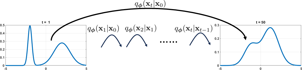
Figure 11: The difference between $q_{\boldsymbol{\phi}}(\mathbf{x}_{t}|\mathbf{x}_{t-1})$ and $q_{\boldsymbol{\phi}}(\mathbf{x}_{t}|\mathbf{x}_{0})$.

Example. For a Gaussian mixture model such that $\mathbf{x}\sim p_{0}(\mathbf{x})=\sum_{k=1}^{K}\pi_{k}\mathcal{N}(\mathbf{x}|\boldsymbol{\mu}_{k},\sigma_{k}^{2}\mathbf{I})$, we can show that the distribution at time $t$ is $\displaystyle p_{t}(\mathbf{x})$ $\displaystyle=\sum_{k=1}^{K}\pi_{k}\mathcal{N}(\mathbf{x}\;|\;\sqrt{\overline{\alpha}_{t}}\boldsymbol{\mu}_{k},(1-\overline{\alpha}_{t})\mathbf{I}+\overline{\alpha}_{t}\sigma_{k}^{2}\mathbf{I})$ (26) $\displaystyle=\sum_{k=1}^{K}\pi_{k}\mathcal{N}(\mathbf{x}\;|\;\sqrt{\alpha^{t}}\boldsymbol{\mu}_{k},(1-\alpha^{t})\mathbf{I}+\alpha^{t}\sigma_{k}^{2}\mathbf{I}),\qquad\text{if }\;\alpha_{t}=\alpha\;\;\text{so that }\;\overline{\alpha}_{t}=\prod_{i=1}^{t}\alpha=\alpha^{t}.$

If you are curious about how the probability distribution $p_{t}$ evolves over time $t$, we show in Figure 12 the trajectory of the distribution. You can see that when we are at $t=0$, the initial distribution is a mixture of two Gaussians. As we progress by following the transition defined in Eqn (26), we can see that the distribution gradually becomes the single Gaussian $\mathcal{N}(0,1)$.

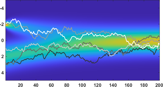
Figure 12: Trajectory plot of the Gaussian mixture, as we progress to transit the probability distribution to $\mathcal{N}(0,1)$.

In the same plot, we overlay and show a few instantaneous trajectories of the random samples $\mathbf{x}_{t}$ as a function of time $t$. The equation we used to generate the samples is

$$\mathbf{x}_{t}=\sqrt{\alpha_{t}}\mathbf{x}_{t-1}+\sqrt{1-\alpha_{t}}\boldsymbol{\epsilon}_{t-1},\qquad\boldsymbol{\epsilon}\sim\mathcal{N}(0,\mathbf{I}).$$

As you can see, the trajectories of $\mathbf{x}_{t}$ more or less follow the distribution $p_{t}(\mathbf{x})$.

2.4 Evidence Lower Bound

Now that we understand the structure of the variational diffusion model, we can write down the ELBO and hence train the model. The ELBO for the variational diffusion model is $\displaystyle\text{ELBO}_{\boldsymbol{\phi},\boldsymbol{\theta}}(\mathbf{x})$ $\displaystyle=\mathbb{E}_{q_{\boldsymbol{\phi}}(\mathbf{x}_{1}|\mathbf{x}_{0})}\Big{[}\log\underset{\text{how good the initial block is}}{\underbrace{p_{\boldsymbol{\theta}}(\mathbf{x}_{0}|\mathbf{x}_{1})}}\Big{]}$ $\displaystyle\qquad-\mathbb{E}_{q_{\boldsymbol{\phi}}(\mathbf{x}_{T-1}|\mathbf{x}_{0})}\Big{[}\underset{\text{how good the final block is}}{\underbrace{\mathbb{D}_{\text{KL}}\Big{(}q_{\boldsymbol{\phi}}(\mathbf{x}_{T}|\mathbf{x}_{T-1})\|p(\mathbf{x}_{T})\Big{)}}}\Big{]}$ $\displaystyle\qquad-\sum_{t=1}^{T-1}\mathbb{E}_{q_{\boldsymbol{\phi}}(\mathbf{x}_{t-1},\mathbf{x}_{t+1}|\mathbf{x}_{0})}\Big{[}\underset{\text{how good the transition blocks are}}{\underbrace{\mathbb{D}_{\text{KL}}\Big{(}q_{\boldsymbol{\phi}}(\mathbf{x}_{t}|\mathbf{x}_{t-1})\|p_{\boldsymbol{\theta}}(\mathbf{x}_{t}|\mathbf{x}_{t+1})\Big{)}}}\Big{]}.$ (27) We can interpret the meaning of this ELBO. The ELBO here consists of three components:

• Reconstruction. The reconstruction term is based on the initial block. We use the log-likelihood $p_{\boldsymbol{\theta}}(\mathbf{x}_{0}|\mathbf{x}_{1})$ to measure how good the neural network associated with $p_{\boldsymbol{\theta}}$ can recover the image $\mathbf{x}_{0}$ from the latent variable $\mathbf{x}_{1}$. The expectation is taken with respect to the samples drawn from $q_{\boldsymbol{\phi}}(\mathbf{x}_{1}|\mathbf{x}_{0})$ which is the distribution that generates $\mathbf{x}_{1}$. If you are puzzled why we want to draw samples from $q_{\boldsymbol{\phi}}(\mathbf{x}_{1}|\mathbf{x}_{0})$, just think about that where the samples $\mathbf{x}_{1}$ should come from. The samples $\mathbf{x}_{1}$ do not come from the sky. Since they are the intermediate latent variables, they are created by the forward transition $q_{\boldsymbol{\phi}}(\mathbf{x}_{1}|\mathbf{x}_{0})$. So, we should generate samples from $q_{\boldsymbol{\phi}}(\mathbf{x}_{1}|\mathbf{x}_{0})$.

• Prior Matching. The prior matching term is based on the final block. We use KL divergence to measure the difference between $q_{\boldsymbol{\phi}}(\mathbf{x}_{T}|\mathbf{x}_{T-1})$ and $p(\mathbf{x}_{T})$. The first distribution $q_{\boldsymbol{\phi}}(\mathbf{x}_{T}|\mathbf{x}_{T-1})$ is the forward transition from $\mathbf{x}_{T-1}$ to $\mathbf{x}_{T}$. This is how $\mathbf{x}_{T}$ is generated. The second distribution is $p(\mathbf{x}_{T})$. Because of our laziness, $p(\mathbf{x}_{T})$ is $\mathcal{N}(0,\mathbf{I})$. We want $q_{\boldsymbol{\phi}}(\mathbf{x}_{T}|\mathbf{x}_{T-1})$ to be as close to $\mathcal{N}(0,\mathbf{I})$ as possible. The samples here are $\mathbf{x}_{T-1}$ which are drawn from $q_{\boldsymbol{\phi}}(\mathbf{x}_{T-1}|\mathbf{x}_{0})$ because $q_{\boldsymbol{\phi}}(\mathbf{x}_{T-1}|\mathbf{x}_{0})$ provides the forward sample generation process.

• Consistency. The consistency term is based on the transition blocks. There are two directions. The forward transition is determined by the distribution $q_{\boldsymbol{\phi}}(\mathbf{x}_{t}|\mathbf{x}_{t-1})$ whereas the reverse transition is determined by the neural network $p_{\boldsymbol{\theta}}(\mathbf{x}_{t}|\mathbf{x}_{t+1})$. The consistency term uses the KL divergence to measure the deviation. The expectation is taken with respect to samples $(\mathbf{x}_{t-1},\mathbf{x}_{t+1})$ drawn from the joint distribution $q_{\boldsymbol{\phi}}(\mathbf{x}_{t-1},\mathbf{x}_{t+1}|\mathbf{x}_{0})$. Oh, what is $q_{\boldsymbol{\phi}}(\mathbf{x}_{t-1},\mathbf{x}_{t+1}|\mathbf{x}_{0})$? No worries. We will get rid of it soon.

At this moment, we will skip the training and inference because this formulation is not ready for implementation. We will discuss one more tricks, and then we will talk about the implementation.

Proof of Eqn (27). Let’s define the following notation: $\mathbf{x}_{0:T}=\{\mathbf{x}_{0},\ldots,\mathbf{x}_{T}\}$ means the collection of all state variables from $t=0$ to $t=T$. We also recall that the prior distribution $p(\mathbf{x})$ is the distribution for the image $\mathbf{x}_{0}$. So it is equivalent to $p(\mathbf{x}_{0})$. With these in mind, we can show that $\displaystyle\log p(\mathbf{x})$ $\displaystyle=\log p(\mathbf{x}_{0})$ $\displaystyle=\log\int p(\mathbf{x}_{0:T})d\mathbf{x}_{1:T}$ Marginalize by integrating over $\mathbf{x}_{1:T}$ $\displaystyle=\log\int p(\mathbf{x}_{0:T})\frac{{\color[rgb]{0,0,1}q_{\boldsymbol{\phi}}(\mathbf{x}_{1:T}|\mathbf{x}_{0})}}{{\color[rgb]{0,0,1}q_{\boldsymbol{\phi}}(\mathbf{x}_{1:T}|\mathbf{x}_{0})}}d\mathbf{x}_{1:T}$ Multiply and divide $q_{\boldsymbol{\phi}}(\mathbf{x}_{1:T}|\mathbf{x}_{0})$ $\displaystyle=\log\int{\color[rgb]{0,0,1}q_{\boldsymbol{\phi}}(\mathbf{x}_{1:T}|\mathbf{x}_{0})}\left[\frac{p(\mathbf{x}_{0:T})}{{\color[rgb]{0,0,1}q_{\boldsymbol{\phi}}(\mathbf{x}_{1:T}|\mathbf{x}_{0})}}\right]d\mathbf{x}_{1:T}$ Rearrange terms $\displaystyle=\log\mathbb{E}_{{\color[rgb]{0,0,1}q_{\boldsymbol{\phi}}(\mathbf{x}_{1:T}|\mathbf{x}_{0})}}\left[\frac{p(\mathbf{x}_{0:T})}{{\color[rgb]{0,0,1}q_{\boldsymbol{\phi}}(\mathbf{x}_{1:T}|\mathbf{x}_{0})}}\right]$ $\displaystyle\text{Definition of expectation}.$ Now, we need to use Jensen’s inequality, which states that for any random variable $X$ and any concave function $f$, it holds that $f(\mathbb{E}[X])\geq\mathbb{E}[f(X)]$. By recognizing that $f(\cdot)=\log(\cdot)$, we can show that $\displaystyle\log p(\mathbf{x})$ $\displaystyle=\log\mathbb{E}_{q_{\boldsymbol{\phi}}(\mathbf{x}_{1:T}|\mathbf{x}_{0})}\left[\frac{p(\mathbf{x}_{0:T})}{q_{\boldsymbol{\phi}}(\mathbf{x}_{1:T}|\mathbf{x}_{0})}\right]$ $\displaystyle\geq\mathbb{E}_{q_{\boldsymbol{\phi}}(\mathbf{x}_{1:T}|\mathbf{x}_{0})}\left[\log\frac{p(\mathbf{x}_{0:T})}{q_{\boldsymbol{\phi}}(\mathbf{x}_{1:T}|\mathbf{x}_{0})}\right]$ (28) Let’s take a closer look at $p(\mathbf{x}_{0:T})$. Inspecting Figure 8, we notice that if we want to decouple $p(\mathbf{x}_{0:T})$, we should do conditioning for $\mathbf{x}_{t-1}|\mathbf{x}_{t}$. This leads to: $\displaystyle p(\mathbf{x}_{0:T})=p(\mathbf{x}_{T})\prod_{t=1}^{T}p(\mathbf{x}_{t-1}|\mathbf{x}_{t})=p(\mathbf{x}_{T})p(\mathbf{x}_{0}|\mathbf{x}_{1})\prod_{t=2}^{T}p(\mathbf{x}_{t-1}|\mathbf{x}_{t}).$ (29) As for $q_{\boldsymbol{\phi}}(\mathbf{x}_{1:T}|\mathbf{x}_{0})$, Figure 8 suggests that we need to do the conditioning for $\mathbf{x}_{t}|\mathbf{x}_{t-1}$. However, because of the sequential relationship, we can write $\displaystyle q_{\boldsymbol{\phi}}(\mathbf{x}_{1:T}|\mathbf{x}_{0})$ $\displaystyle=\prod_{t=1}^{T}q_{\boldsymbol{\phi}}(\mathbf{x}_{t}|\mathbf{x}_{t-1})=q_{\boldsymbol{\phi}}(\mathbf{x}_{T}|\mathbf{x}_{T-1})\prod_{t=1}^{T-1}q_{\boldsymbol{\phi}}(\mathbf{x}_{t}|\mathbf{x}_{t-1}).$ (30) Substituting Eqn (29) and Eqn (30) back to Eqn (28), we can show that $\displaystyle\log p(\mathbf{x})$ $\displaystyle\geq\mathbb{E}_{q_{\boldsymbol{\phi}}(\mathbf{x}_{1:T}|\mathbf{x}_{0})}\left[\log\frac{p(\mathbf{x}_{0:T})}{q_{\boldsymbol{\phi}}(\mathbf{x}_{1:T}|\mathbf{x}_{0})}\right]$ $\displaystyle=\mathbb{E}_{q_{\boldsymbol{\phi}}(\mathbf{x}_{1:T}|\mathbf{x}_{0})}\left[\log\frac{{\color[rgb]{0,0,1}p(\mathbf{x}_{T})p(\mathbf{x}_{0}|\mathbf{x}_{1})\prod_{t=2}^{T}p(\mathbf{x}_{t-1}|\mathbf{x}_{t})}}{{\color[rgb]{0,0,1}q_{\boldsymbol{\phi}}(\mathbf{x}_{T}|\mathbf{x}_{T-1})\prod_{t=1}^{T-1}q_{\boldsymbol{\phi}}(\mathbf{x}_{t}|\mathbf{x}_{t-1})}}\right]$ $\displaystyle=\mathbb{E}_{q_{\boldsymbol{\phi}}(\mathbf{x}_{1:T}|\mathbf{x}_{0})}\left[\log\frac{p(\mathbf{x}_{T})p(\mathbf{x}_{0}|\mathbf{x}_{1}){\color[rgb]{0,0,1}\prod_{t=1}^{T-1}p(\mathbf{x}_{t}|\mathbf{x}_{t+1})}}{q_{\boldsymbol{\phi}}(\mathbf{x}_{T}|\mathbf{x}_{T-1})\prod_{t=1}^{T-1}q_{\boldsymbol{\phi}}(\mathbf{x}_{t}|\mathbf{x}_{t-1})}\right]$ shift $t$ to $t+1$ $\displaystyle=\mathbb{E}_{q_{\boldsymbol{\phi}}(\mathbf{x}_{1:T}|\mathbf{x}_{0})}\left[\log\frac{p(\mathbf{x}_{T})p(\mathbf{x}_{0}|\mathbf{x}_{1})}{q_{\boldsymbol{\phi}}(\mathbf{x}_{T}|\mathbf{x}_{T-1})}\right]+\mathbb{E}_{q_{\boldsymbol{\phi}}(\mathbf{x}_{1:T}|\mathbf{x}_{0})}\left[\log\prod_{t=1}^{T-1}\frac{p(\mathbf{x}_{t}|\mathbf{x}_{t+1})}{q_{\boldsymbol{\phi}}(\mathbf{x}_{t}|\mathbf{x}_{t-1})}\right]$ split expectation The first term above can be further decomposed into two expectations $\displaystyle\mathbb{E}_{q_{\boldsymbol{\phi}}(\mathbf{x}_{1:T}|\mathbf{x}_{0})}\left[\log\frac{p(\mathbf{x}_{T})p(\mathbf{x}_{0}|\mathbf{x}_{1})}{q_{\boldsymbol{\phi}}(\mathbf{x}_{T}|\mathbf{x}_{T-1})}\right]$ $\displaystyle=\underset{\text{Reconstruction}}{\underbrace{\mathbb{E}_{q_{\boldsymbol{\phi}}(\mathbf{x}_{1:T}|\mathbf{x}_{0})}\bigg{[}\log p(\mathbf{x}_{0}|\mathbf{x}_{1})\bigg{]}}}+\underset{\text{Prior Matching}}{\underbrace{\mathbb{E}_{q_{\boldsymbol{\phi}}(\mathbf{x}_{1:T}|\mathbf{x}_{0})}\left[\log\frac{p(\mathbf{x}_{T})}{q_{\boldsymbol{\phi}}(\mathbf{x}_{T}|\mathbf{x}_{T-1})}\right]}}.$ The Reconstruction term can be simplified as $\displaystyle\mathbb{E}_{q_{\boldsymbol{\phi}}(\mathbf{x}_{1:T}|\mathbf{x}_{0})}\bigg{[}\log p(\mathbf{x}_{0}|\mathbf{x}_{1})\bigg{]}$ $\displaystyle=\mathbb{E}_{q_{\boldsymbol{\phi}}(\mathbf{x}_{1}|\mathbf{x}_{0})}\bigg{[}\log p(\mathbf{x}_{0}|\mathbf{x}_{1})\bigg{]},$ where we used the fact that the conditioning $\mathbf{x}_{1:T}|\mathbf{x}_{0}$ is equivalent to $\mathbf{x}_{1}|\mathbf{x}_{0}$. The Prior Matching term is $\displaystyle\mathbb{E}_{q_{\boldsymbol{\phi}}(\mathbf{x}_{1:T}|\mathbf{x}_{0})}\left[\log\frac{p(\mathbf{x}_{T})}{q_{\boldsymbol{\phi}}(\mathbf{x}_{T}|\mathbf{x}_{T-1})}\right]$ $\displaystyle=\mathbb{E}_{q_{\boldsymbol{\phi}}(\mathbf{x}_{T},\mathbf{x}_{T-1}|\mathbf{x}_{0})}\left[\log\frac{p(\mathbf{x}_{T})}{q_{\boldsymbol{\phi}}(\mathbf{x}_{T}|\mathbf{x}_{T-1})}\right]$ $\displaystyle=-\mathbb{E}_{q_{\boldsymbol{\phi}}(\mathbf{x}_{T-1},\mathbf{x}_{T}|\mathbf{x}_{0})}\Bigg{[}\mathbb{D}_{\text{KL}}\left(q_{\boldsymbol{\phi}}(\mathbf{x}_{T}|\mathbf{x}_{T-1})\|p(\mathbf{x}_{T})\right)\Bigg{]},$ where we notice that the conditional expectation can be simplified to samples $\mathbf{x}_{T}$ and $\mathbf{x}_{T-1}$ only, because $\log\frac{p(\mathbf{x}_{T})}{q_{\boldsymbol{\phi}}(\mathbf{x}_{T}|\mathbf{x}_{T-1})}$ only depends on $\mathbf{x}_{T}$ and $\mathbf{x}_{T-1}$. Finally, we look at the product term. We can show that $\displaystyle\mathbb{E}_{q_{\boldsymbol{\phi}}(\mathbf{x}_{1:T}|\mathbf{x}_{0})}\left[\log\prod_{t=1}^{T-1}\frac{p(\mathbf{x}_{t}|\mathbf{x}_{t+1})}{q_{\boldsymbol{\phi}}(\mathbf{x}_{t}|\mathbf{x}_{t-1})}\right]$ $\displaystyle=\sum_{t=1}^{T-1}\mathbb{E}_{q_{\boldsymbol{\phi}}(\mathbf{x}_{1:T}|\mathbf{x}_{0})}\left[\log\frac{p(\mathbf{x}_{t}|\mathbf{x}_{t+1})}{q_{\boldsymbol{\phi}}(\mathbf{x}_{t}|\mathbf{x}_{t-1})}\right]$ $\displaystyle=\sum_{t=1}^{T-1}\mathbb{E}_{q_{\boldsymbol{\phi}}(\mathbf{x}_{t-1},\mathbf{x}_{t},\mathbf{x}_{t+1}|\mathbf{x}_{0})}\left[\log\frac{p(\mathbf{x}_{t}|\mathbf{x}_{t+1})}{q_{\boldsymbol{\phi}}(\mathbf{x}_{t}|\mathbf{x}_{t-1})}\right]$ $\displaystyle=\underset{\text{consistency}}{\underbrace{-\sum_{t=1}^{T-1}\mathbb{E}_{q_{\boldsymbol{\phi}}(\mathbf{x}_{t-1},\mathbf{x}_{t+1}|\mathbf{x}_{0})}\Bigg{[}\mathbb{D}_{\text{KL}}\left(q_{\boldsymbol{\phi}}(\mathbf{x}_{t}|\mathbf{x}_{t-1})\|p(\mathbf{x}_{t}|\mathbf{x}_{t+1})\right)\Bigg{]}}}.$ By replacing $p(\mathbf{x}_{0}|\mathbf{x}_{1})$ with $p_{\boldsymbol{\theta}}(\mathbf{x}_{0}|\mathbf{x}_{1})$ and $p(\mathbf{x}_{t}|\mathbf{x}_{t+1})$ with $p_{\boldsymbol{\theta}}(\mathbf{x}_{t}|\mathbf{x}_{t+1})$, we are done.

2.5 Rewrite the Consistency Term

The nightmare of the above variation diffusion model is that we need to draw samples $(\mathbf{x}_{t-1},\mathbf{x}_{t+1})$ from a joint distribution $q_{\boldsymbol{\phi}}(\mathbf{x}_{t-1},\mathbf{x}_{t+1}|\mathbf{x}_{0})$. We don’t know what $q_{\boldsymbol{\phi}}(\mathbf{x}_{t-1},\mathbf{x}_{t+1}|\mathbf{x}_{0})$ is! Well, it is a Gaussian, of course, but still we need to use future samples $\mathbf{x}_{t+1}$ to draw the current sample $\mathbf{x}_{t}$. This is odd, and it is not fun.

Inspecting the consistency term, we notice that $q_{\boldsymbol{\phi}}(\mathbf{x}_{t}|\mathbf{x}_{t-1})$ and $p_{\boldsymbol{\theta}}(\mathbf{x}_{t}|\mathbf{x}_{t+1})$ are moving along two opposite directions. Thus, it is unavoidable that we need to use $\mathbf{x}_{t-1}$ and $\mathbf{x}_{t+1}$. The question we need to ask is: Can we come up with something so that we do not need to handle two opposite directions while we are able to check consistency?

So, here is the simple trick called Bayes theorem.

$$q(\mathbf{x}_{t}|\mathbf{x}_{t-1})=\frac{q(\mathbf{x}_{t-1}|\mathbf{x}_{t})q(\mathbf{x}_{t})}{q(\mathbf{x}_{t-1})}\quad\overset{\text{\scriptsize{condition on $\mathbf{x}_{0}$}}}{\Longrightarrow}\quad q(\mathbf{x}_{t}|\mathbf{x}_{t-1},{\color[rgb]{0,0,1}\mathbf{x}_{0}})=\frac{q(\mathbf{x}_{t-1}|\mathbf{x}_{t},{\color[rgb]{0,0,1}\mathbf{x}_{0}})q(\mathbf{x}_{t}|{\color[rgb]{0,0,1}\mathbf{x}_{0}})}{q(\mathbf{x}_{t-1}|{\color[rgb]{0,0,1}\mathbf{x}_{0}})}.$$ (31)

With this change of the conditioning order, we can switch $q(\mathbf{x}_{t}|\mathbf{x}_{t-1},\mathbf{x}_{0})$ to $q(\mathbf{x}_{t-1}|\mathbf{x}_{t},\mathbf{x}_{0})$ by adding one more condition variable $\mathbf{x}_{0}$. The direction $q(\mathbf{x}_{t-1}|\mathbf{x}_{t},\mathbf{x}_{0})$ is now parallel to $p_{\boldsymbol{\theta}}(\mathbf{x}_{t-1}|\mathbf{x}_{t})$ as shown in Figure 13. So, if we want to rewrite the consistency term, a natural option is to calculate the KL divergence between $q_{\boldsymbol{\phi}}(\mathbf{x}_{t-1}|\mathbf{x}_{t},\mathbf{x}_{0})$ and $p_{\boldsymbol{\theta}}(\mathbf{x}_{t-1}|\mathbf{x}_{t})$.

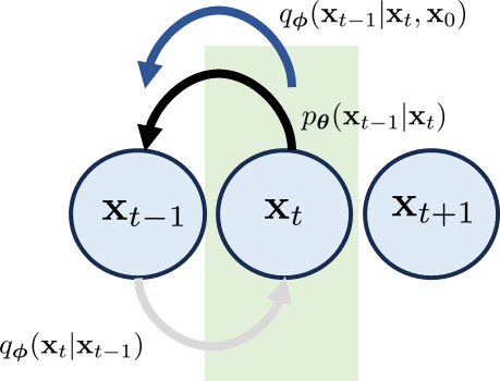
Figure 13: If we consider the Bayes theorem in Eqn (31), we can define a distribution $q_{\boldsymbol{\phi}}(\mathbf{x}_{t-1}|\mathbf{x}_{t},\mathbf{x}_{0})$ that has a direction parallel to $p_{\boldsymbol{\theta}}(\mathbf{x}_{t-1}|\mathbf{x}_{t})$.

If we manage to go through a few (boring) algebraic derivations, we can show that the ELBO is now: The ELBO for a variational diffusion model is $\displaystyle\text{ELBO}_{\boldsymbol{\phi},\boldsymbol{\theta}}(\mathbf{x})$ $\displaystyle=\mathbb{E}_{q_{\boldsymbol{\phi}}(\mathbf{x}_{1}|\mathbf{x}_{0})}[\log\underset{\text{same as before}}{\underbrace{p_{\boldsymbol{\theta}}(\mathbf{x}_{0}|\mathbf{x}_{1})}}]-\underset{\text{new prior matching}}{\underbrace{\mathbb{D}_{\text{KL}}\Big{(}q_{\boldsymbol{\phi}}(\mathbf{x}_{T}|\mathbf{x}_{0})\|p(\mathbf{x}_{T})\Big{)}}}$ $\displaystyle\qquad-\sum_{t=2}^{T}\mathbb{E}_{q_{\boldsymbol{\phi}}(\mathbf{x}_{t}|\mathbf{x}_{0})}\Big{[}\underset{\text{new consistency}}{\underbrace{\mathbb{D}_{\text{KL}}\Big{(}q_{\boldsymbol{\phi}}(\mathbf{x}_{t-1}|\mathbf{x}_{t},\mathbf{x}_{0})\|p_{\boldsymbol{\theta}}(\mathbf{x}_{t-1}|\mathbf{x}_{t})\Big{)}}}\Big{]}.$ (32) Let’s quickly make three interpretations:

• Reconstruction. The new reconstruction term is the same as before. We are still maximizing the log-likelihood.

• Prior Matching. The new prior matching is simplified to the KL divergence between $q_{\boldsymbol{\phi}}(\mathbf{x}_{T}|\mathbf{x}_{0})$ and $p(\mathbf{x}_{T})$. The change is due to the fact that we now condition upon $\mathbf{x}_{0}$. Thus, there is no need to draw samples from $q_{\boldsymbol{\phi}}(\mathbf{x}_{T-1}|\mathbf{x}_{0})$ and take expectation.

• Consistency. The new consistency term is different from the previous one in two ways. Firstly, the running index $t$ starts at $t=2$ and ends at $t=T$. Previously it was from $t=1$ to $t=T-1$. Accompanied with this is the distribution matching, which is now between $q_{\boldsymbol{\phi}}(\mathbf{x}_{t-1}|\mathbf{x}_{t},\mathbf{x}_{0})$ and $p_{\boldsymbol{\theta}}(\mathbf{x}_{t-1}|\mathbf{x}_{t})$. So, instead of asking a forward transition to match with a reverse transition, we use $q_{\boldsymbol{\phi}}$ to construct a reverse transition and use it to match with $p_{\boldsymbol{\theta}}$.

Proof of Eqn (32). We begin with Eqn (28) by showing that $\displaystyle\log p(\mathbf{x})$ $\displaystyle\geq\mathbb{E}_{q_{\boldsymbol{\phi}}(\mathbf{x}_{1:T}|\mathbf{x}_{0})}\left[\log\frac{p(\mathbf{x}_{0:T})}{q_{\boldsymbol{\phi}}(\mathbf{x}_{1:T}|\mathbf{x}_{0})}\right]$ By Eqn (28) $\displaystyle=\mathbb{E}_{q_{\boldsymbol{\phi}}(\mathbf{x}_{1:T}|\mathbf{x}_{0})}\left[\log\frac{p(\mathbf{x}_{T})p(\mathbf{x}_{0}|\mathbf{x}_{1})\prod_{t=2}^{T}p(\mathbf{x}_{t-1}|\mathbf{x}_{t})}{q_{\boldsymbol{\phi}}(\mathbf{x}_{1}|\mathbf{x}_{0})\prod_{t=2}^{T}q_{\boldsymbol{\phi}}(\mathbf{x}_{t}|\mathbf{x}_{t-1},\mathbf{x}_{0})}\right]$ split the chain $\displaystyle=\mathbb{E}_{q_{\boldsymbol{\phi}}(\mathbf{x}_{1:T}|\mathbf{x}_{0})}\left[\log\frac{p(\mathbf{x}_{T})p(\mathbf{x}_{0}|\mathbf{x}_{1})}{q_{\boldsymbol{\phi}}(\mathbf{x}_{1}|\mathbf{x}_{0})}\right]+\mathbb{E}_{q_{\boldsymbol{\phi}}(\mathbf{x}_{1:T}|\mathbf{x}_{0})}\left[\log\prod_{t=2}^{T}\frac{p(\mathbf{x}_{t-1}|\mathbf{x}_{t})}{q_{\boldsymbol{\phi}}(\mathbf{x}_{t}|\mathbf{x}_{t-1},\mathbf{x}_{0})}\right]$ (33) Let’s consider the second term: $\displaystyle\prod_{t=2}^{T}\frac{p(\mathbf{x}_{t-1}|\mathbf{x}_{t})}{q_{\boldsymbol{\phi}}(\mathbf{x}_{t}|\mathbf{x}_{t-1},\mathbf{x}_{0})}$ $\displaystyle=\prod_{t=2}^{T}\frac{p(\mathbf{x}_{t-1}|\mathbf{x}_{t})}{\frac{q_{\boldsymbol{\phi}}(\mathbf{x}_{t-1}|\mathbf{x}_{t},\mathbf{x}_{0})q_{\boldsymbol{\phi}}(\mathbf{x}_{t}|\mathbf{x}_{0})}{q_{\boldsymbol{\phi}}(\mathbf{x}_{t-1}|\mathbf{x}_{0})}}$ Bayes rule, Eqn (31) $\displaystyle=\prod_{t=2}^{T}\frac{p(\mathbf{x}_{t-1}|\mathbf{x}_{t})}{q_{\boldsymbol{\phi}}(\mathbf{x}_{t-1}|\mathbf{x}_{t},\mathbf{x}_{0})}\times\prod_{t=2}^{T}\frac{q_{\boldsymbol{\phi}}(\mathbf{x}_{t-1}|\mathbf{x}_{0})}{q_{\boldsymbol{\phi}}(\mathbf{x}_{t}|\mathbf{x}_{0})}$ Rearrange denominator $\displaystyle=\prod_{t=2}^{T}\frac{p(\mathbf{x}_{t-1}|\mathbf{x}_{t})}{q_{\boldsymbol{\phi}}(\mathbf{x}_{t-1}|\mathbf{x}_{t},\mathbf{x}_{0})}\times\frac{q_{\boldsymbol{\phi}}(\mathbf{x}_{1}|\mathbf{x}_{0})}{q_{\boldsymbol{\phi}}(\mathbf{x}_{T}|\mathbf{x}_{0})},$ Recursion cancels terms where the last equation uses the fact that for any sequence $a_{1},\ldots,a_{T}$, we have $\prod_{t=2}^{T}\frac{a_{t-1}}{a_{t}}=\frac{a_{1}}{a_{2}}\times\frac{a_{2}}{a_{3}}\times\ldots\times\frac{a_{T-1}}{a_{T}}=\frac{a_{1}}{a_{T}}$. Going back to the Eqn (33), we can see that $\displaystyle\mathbb{E}_{q_{\boldsymbol{\phi}}(\mathbf{x}_{1:T}|\mathbf{x}_{0})}\left[\log\frac{p(\mathbf{x}_{T})p(\mathbf{x}_{0}|\mathbf{x}_{1})}{q_{\boldsymbol{\phi}}(\mathbf{x}_{1}|\mathbf{x}_{0})}\right]+\mathbb{E}_{q_{\boldsymbol{\phi}}(\mathbf{x}_{1:T}|\mathbf{x}_{0})}\left[\log\prod_{t=2}^{T}\frac{p(\mathbf{x}_{t-1}|\mathbf{x}_{t})}{q_{\boldsymbol{\phi}}(\mathbf{x}_{t}|\mathbf{x}_{t-1},\mathbf{x}_{0})}\right]$ $\displaystyle=\mathbb{E}_{q_{\boldsymbol{\phi}}(\mathbf{x}_{1:T}|\mathbf{x}_{0})}\left[\log\frac{p(\mathbf{x}_{T})p(\mathbf{x}_{0}|\mathbf{x}_{1})}{q_{\boldsymbol{\phi}}(\mathbf{x}_{1}|\mathbf{x}_{0})}+\log\frac{q_{\boldsymbol{\phi}}(\mathbf{x}_{1}|\mathbf{x}_{0})}{q_{\boldsymbol{\phi}}(\mathbf{x}_{T}|\mathbf{x}_{0})}\right]+\mathbb{E}_{q_{\boldsymbol{\phi}}(\mathbf{x}_{1:T}|\mathbf{x}_{0})}\left[\log\prod_{t=2}^{T}\frac{p(\mathbf{x}_{t-1}|\mathbf{x}_{t})}{q_{\boldsymbol{\phi}}(\mathbf{x}_{t-1}|\mathbf{x}_{t},\mathbf{x}_{0})}\right]$ $\displaystyle=\mathbb{E}_{q_{\boldsymbol{\phi}}(\mathbf{x}_{1:T}|\mathbf{x}_{0})}\left[\log\frac{p(\mathbf{x}_{T})p(\mathbf{x}_{0}|\mathbf{x}_{1})}{q_{\boldsymbol{\phi}}(\mathbf{x}_{T}|\mathbf{x}_{0})}\right]+\mathbb{E}_{q_{\boldsymbol{\phi}}(\mathbf{x}_{1:T}|\mathbf{x}_{0})}\left[\log\prod_{t=2}^{T}\frac{p(\mathbf{x}_{t-1}|\mathbf{x}_{t})}{q_{\boldsymbol{\phi}}(\mathbf{x}_{t-1}|\mathbf{x}_{t},\mathbf{x}_{0})}\right],$ where we canceled $q_{\boldsymbol{\phi}}(\mathbf{x}_{1}|\mathbf{x}_{0})$ in the numerator and denominator since $\log\frac{a}{b}+\log\frac{b}{c}=\log\frac{a}{c}$ for any positive constants $a$, $b$, and $c$. This will give us $\displaystyle\mathbb{E}_{q_{\boldsymbol{\phi}}(\mathbf{x}_{1:T}|\mathbf{x}_{0})}\left[\log\frac{p(\mathbf{x}_{T})p(\mathbf{x}_{0}|\mathbf{x}_{1})}{q_{\boldsymbol{\phi}}(\mathbf{x}_{T}|\mathbf{x}_{0})}\right]$ $\displaystyle=\mathbb{E}_{q_{\boldsymbol{\phi}}(\mathbf{x}_{1:T}|\mathbf{x}_{0})}\left[\log p(\mathbf{x}_{0}|\mathbf{x}_{1})\right]+\mathbb{E}_{q_{\boldsymbol{\phi}}(\mathbf{x}_{1:T}|\mathbf{x}_{0})}\left[\log\frac{p(\mathbf{x}_{T})}{q_{\boldsymbol{\phi}}(\mathbf{x}_{T}|\mathbf{x}_{0})}\right]$ $\displaystyle=\underset{\text{reconstruction}}{\underbrace{\mathbb{E}_{q_{\boldsymbol{\phi}}(\mathbf{x}_{1}|\mathbf{x}_{0})}\left[\log p(\mathbf{x}_{0}|\mathbf{x}_{1})\right]}}-\underset{\text{prior matching}}{\underbrace{\mathbb{D}_{\text{KL}}(q_{\boldsymbol{\phi}}(\mathbf{x}_{T}|\mathbf{x}_{0})\|p(\mathbf{x}_{T}))}}.$ The last term is $\displaystyle\mathbb{E}_{q_{\boldsymbol{\phi}}(\mathbf{x}_{1:T}|\mathbf{x}_{0})}\left[\log\prod_{t=2}^{T}\frac{p(\mathbf{x}_{t-1}|\mathbf{x}_{t})}{q_{\boldsymbol{\phi}}(\mathbf{x}_{t-1}|\mathbf{x}_{t},\mathbf{x}_{0})}\right]$ $\displaystyle=\sum_{t=2}\mathbb{E}_{q_{\boldsymbol{\phi}}(\mathbf{x}_{t},\mathbf{x}_{t-1}|\mathbf{x}_{0})}\log\frac{p(\mathbf{x}_{t-1}|\mathbf{x}_{t})}{q_{\boldsymbol{\phi}}(\mathbf{x}_{t-1}|\mathbf{x}_{t},\mathbf{x}_{0})}$ $\displaystyle=-\underset{\text{consistency}}{\underbrace{\sum_{t=2}\mathbb{E}_{q_{\boldsymbol{\phi}}(\mathbf{x}_{t},\mathbf{x}_{t-1}|\mathbf{x}_{0})}\mathbb{D}_{\text{KL}}(q_{\boldsymbol{\phi}}(\mathbf{x}_{t-1}|\mathbf{x}_{t},\mathbf{x}_{0})\|p(\mathbf{x}_{t-1}|\mathbf{x}_{t}))}}.$ Finally, replace $p(\mathbf{x}_{t-1}|\mathbf{x}_{t})$ by $p_{\boldsymbol{\theta}}(\mathbf{x}_{t-1}|\mathbf{x}_{t})$, and $p(\mathbf{x}_{0}|\mathbf{x}_{1})$ by $p_{\boldsymbol{\theta}}(\mathbf{x}_{0}|\mathbf{x}_{1})$. Done!

2.6 Derivation of $q_{\boldsymbol{\phi}}(\mathbf{x}_{t-1}|\mathbf{x}_{t},\mathbf{x}_{0})$

Now that we know the new ELBO for the variational diffusion model, we should spend some time discussing its core component which is $q_{\boldsymbol{\phi}}(\mathbf{x}_{t-1}|\mathbf{x}_{t},\mathbf{x}_{0})$. In a nutshell, what we want to show is that

• $q_{\boldsymbol{\phi}}(\mathbf{x}_{t-1}|\mathbf{x}_{t},\mathbf{x}_{0})$ is not as crazy as you think. It is still a Gaussian.

• Since it is a Gaussian, it is fully characterized by the mean and covariance. It turns out that

  $$q_{\boldsymbol{\phi}}(\mathbf{x}_{t-1}|\mathbf{x}_{t},\mathbf{x}_{0})=\mathcal{N}(\mathbf{x}_{t-1}\,|\,\heartsuit\mathbf{x}_{t}+\spadesuit\mathbf{x}_{0},\clubsuit\mathbf{I}),$$ (34)

  for some magical scalars $\heartsuit$, $\spadesuit$ and $\clubsuit$ defined below.

The distribution $q_{\boldsymbol{\phi}}(\mathbf{x}_{t-1}|\mathbf{x}_{t},\mathbf{x}_{0})$ takes the form of $$q_{\boldsymbol{\phi}}(\mathbf{x}_{t-1}|\mathbf{x}_{t},\mathbf{x}_{0})=\mathcal{N}(\mathbf{x}_{t-1}\,|\,\boldsymbol{\mu}_{q}(\mathbf{x}_{t},\mathbf{x}_{0}),\boldsymbol{\Sigma}_{q}(t)),$$ (35) where $\displaystyle\boldsymbol{\mu}_{q}(\mathbf{x}_{t},\mathbf{x}_{0})$ $\displaystyle=\frac{(1-\overline{\alpha}_{t-1})\sqrt{\alpha_{t}}}{1-\overline{\alpha}_{t}}\mathbf{x}_{t}+\frac{(1-\alpha_{t})\sqrt{\overline{\alpha}_{t-1}}}{1-\overline{\alpha}_{t}}\mathbf{x}_{0}$ (36) $\displaystyle\boldsymbol{\Sigma}_{q}(t)$ $\displaystyle=\frac{(1-\alpha_{t})(1-\sqrt{\overline{\alpha}_{t-1}})}{1-\overline{\alpha}_{t}}\mathbf{I}\overset{\text{def}}{=}\sigma_{q}^{2}(t)\mathbf{I}.$ (37)

The interesting part of Eqn (35) is that $q_{\boldsymbol{\phi}}(\mathbf{x}_{t-1}|\mathbf{x}_{t},\mathbf{x}_{0})$ is completely characterized by $\mathbf{x}_{t}$ and $\mathbf{x}_{0}$. There is no neural network required to estimate the mean and variance! (You can compare this with VAE where a network is needed.) Since a network is not needed, there is really nothing to “learn”. The distribution $q_{\boldsymbol{\phi}}(\mathbf{x}_{t-1}|\mathbf{x}_{t},\mathbf{x}_{0})$ is automatically determined if we know $\mathbf{x}_{t}$ and $\mathbf{x}_{0}$. No guessing, no estimation, nothing.

The realization here is important. If we look at the consistency term, it is a summation of many KL divergence terms where the $t$-th term is

$$\mathbb{D}_{\text{KL}}(\underset{\quad\text{nothing to learn}\quad}{\underbrace{q_{\boldsymbol{\phi}}(\mathbf{x}_{t-1}|\mathbf{x}_{t},\mathbf{x}_{0})}}\|\underset{\text{need to do something}}{\underbrace{p_{\boldsymbol{\theta}}(\mathbf{x}_{t-1}|\mathbf{x}_{t})}}).$$ (38)

As we just said, there is nothing to do with $q_{\boldsymbol{\phi}}(\mathbf{x}_{t-1}|\mathbf{x}_{t},\mathbf{x}_{0})$. But we need to do something to $p_{\boldsymbol{\theta}}(\mathbf{x}_{t-1}|\mathbf{x}_{t})$ so that we can calculate the KL divergence.

So, what should we do? We know that $q_{\boldsymbol{\phi}}(\mathbf{x}_{t-1}|\mathbf{x}_{t},\mathbf{x}_{0})$ is Gaussian. If we want to quickly calculate the KL divergence, then obviously we need to assume that $p_{\boldsymbol{\theta}}(\mathbf{x}_{t-1}|\mathbf{x}_{t})$ is also a Gaussian. Yeah, no kidding. We have no justification why it is a Gaussian. But since $p_{\boldsymbol{\theta}}$ is a distribution we can choose, we should of course choose something easier. To this end, we pick

$$p_{\boldsymbol{\theta}}(\mathbf{x}_{t-1}|\mathbf{x}_{t})=\mathcal{N}\Big{(}\mathbf{x}_{t-1}|\underset{\text{neural network}}{\underbrace{\boldsymbol{\mu}_{\boldsymbol{\theta}}(\mathbf{x}_{t})}},\sigma_{q}^{2}(t)\mathbf{I}\Big{)},$$ (39)

where we assume that the mean vector can be determined using a neural network. As for the variance, we choose the variance to be $\sigma_{q}^{2}(t)$. This is identical to Eqn (37)! Thus, if we put Eqn (35) side by side with $p_{\boldsymbol{\theta}}(\mathbf{x}_{t-1}|\mathbf{x}_{t})$, we notice a parallel relation between the two:

$$q_{\boldsymbol{\phi}}(\mathbf{x}_{t-1}|\mathbf{x}_{t},\mathbf{x}_{0}) =\mathcal{N}\Big{(}\mathbf{x}_{t-1}\,|\,\underset{\text{known}}{\underbrace{\boldsymbol{\mu}_{q}(\mathbf{x}_{t},\mathbf{x}_{0})}},\underset{\text{known}}{\underbrace{\sigma_{q}^{2}(t)\mathbf{I}}}\Big{)},$$ (40)

$$p_{\boldsymbol{\theta}}(\mathbf{x}_{t-1}|\mathbf{x}_{t}) =\mathcal{N}\Big{(}\mathbf{x}_{t-1}|\underset{\text{neural network}}{\underbrace{\boldsymbol{\mu}_{\boldsymbol{\theta}}(\mathbf{x}_{t})}},\underset{\text{known}}{\underbrace{\sigma_{q}^{2}(t)\mathbf{I}}}\Big{)}.$$ (41)

Therefore, the KL divergence is simplified to

$$\mathbb{D}_{\text{KL}}\Big{(}q_{\boldsymbol{\phi}}(\mathbf{x}_{t-1}|\mathbf{x}_{t},\mathbf{x}_{0})\|p_{\boldsymbol{\theta}}(\mathbf{x}_{t-1}|\mathbf{x}_{t})\Big{)}$$

$$=\mathbb{D}_{\text{KL}}\Big{(}\mathcal{N}(\mathbf{x}_{t-1}\,|\,\boldsymbol{\mu}_{q}(\mathbf{x}_{t},\mathbf{x}_{0}),\sigma_{q}^{2}(t)\mathbf{I})\|\mathcal{N}(\mathbf{x}_{t-1}\,|\,\boldsymbol{\mu}_{\boldsymbol{\theta}}(\mathbf{x}_{t}),\sigma_{q}^{2}(t)\mathbf{I})\Big{)}$$

$$=\frac{1}{2\sigma_{q}^{2}(t)}\|\boldsymbol{\mu}_{q}(\mathbf{x}_{t},\mathbf{x}_{0})-\boldsymbol{\mu}_{\boldsymbol{\theta}}(\mathbf{x}_{t})\|^{2},$$ (42)

where we used the fact that the KL divergence between two identical-variance Gaussians is just the Euclidean distance square between the two mean vectors.

If we go back to the definition of ELBO in Eqn (32), we can rewrite it as

$$\text{ELBO}_{\boldsymbol{\theta}}(\mathbf{x}) =\mathbb{E}_{q(\mathbf{x}_{1}|\mathbf{x}_{0})}[\log p_{\boldsymbol{\theta}}(\mathbf{x}_{0}|\mathbf{x}_{1})]-\underset{\text{nothing to train}}{\underbrace{\mathbb{D}_{\text{KL}}\Big{(}q(\mathbf{x}_{T}|\mathbf{x}_{0})\|p(\mathbf{x}_{T})\Big{)}}}$$

$$\qquad-\sum_{t=2}^{T}\mathbb{E}_{q(\mathbf{x}_{t}|\mathbf{x}_{0})}\Big{[}\frac{1}{2\sigma_{q}^{2}(t)}\|\boldsymbol{\mu}_{q}(\mathbf{x}_{t},\mathbf{x}_{0})-\boldsymbol{\mu}_{\boldsymbol{\theta}}(\mathbf{x}_{t})\|^{2}\Big{]}.$$ (43)

A few observations are interesting:

• We dropped all the subscripts $\boldsymbol{\phi}$ because $q$ is completely described as long as we know $\mathbf{x}_{0}$. We are just adding (different level of) white noise to each of $\mathbf{x}_{1},\ldots,\mathbf{x}_{T}$. This will give us an ELBO that only requires us to optimize over $\boldsymbol{\theta}$.

• The parameter $\boldsymbol{\theta}$ is realized through the network $\boldsymbol{\mu}_{\boldsymbol{\theta}}(\mathbf{x}_{t})$. It is the network weight for $\boldsymbol{\mu}_{\boldsymbol{\theta}}(\mathbf{x}_{t})$.

• The sampling from $q(\mathbf{x}_{t}|\mathbf{x}_{0})$ is done according to Eqn (21) which states that $q(\mathbf{x}_{t}|\mathbf{x}_{0})=\mathcal{N}(\mathbf{x}_{t}|\sqrt{\overline{\alpha}_{t}}\mathbf{x}_{0},(1-\overline{\alpha}_{t})\mathbf{I})$.

• Given $\mathbf{x}_{t}\sim q(\mathbf{x}_{t}|\mathbf{x}_{0})$, we can calculate $\log p_{\boldsymbol{\theta}}(\mathbf{x}_{0}|\mathbf{x}_{1})$, which is just $\log\mathcal{N}(\mathbf{x}_{0}|\boldsymbol{\mu}_{\boldsymbol{\theta}}(\mathbf{x}_{1}),\sigma_{q}^{2}(1)\mathbf{I})$. So, as soon as we know $\mathbf{x}_{1}$, we can send it to a network $\boldsymbol{\mu}_{\boldsymbol{\theta}}(\mathbf{x}_{1})$ to return us a mean estimate. The mean estimate will then be used to compute the likelihood.

Before we go further down, let’s complete the story by discussing how Eqn (35) was determined.

Proof of Eqn (35). Using the Bayes theorem stated in Eqn (31), $q(\mathbf{x}_{t-1}|\mathbf{x}_{t},\mathbf{x}_{0})$ can be determined if we evaluate the following product of Gaussians $$q(\mathbf{x}_{t-1}|\mathbf{x}_{t},\mathbf{x}_{0})=\frac{\mathcal{N}(\mathbf{x}_{t}|\sqrt{\alpha_{t}}\mathbf{x}_{t-1},(1-\alpha_{t})\mathbf{I})\mathcal{N}(\mathbf{x}_{t-1}|\sqrt{\overline{\alpha}_{t-1}},(1-\overline{\alpha}_{t-1}\mathbf{I}))}{\mathcal{N}(\mathbf{x}_{t}|\sqrt{\overline{\alpha}_{t}}\mathbf{x}_{0},(1-\overline{\alpha}_{t})\mathbf{I})}.$$ (44) For simplicity we will treat the vectors are scalars. Then the above product of Gaussians will become $$q(\mathbf{x}_{t-1}|\mathbf{x}_{t},\mathbf{x}_{0})\propto\exp\left\{\frac{(\mathbf{x}_{t}-\sqrt{\alpha_{t}}\mathbf{x}_{t-1})^{2}}{2(1-\alpha_{t})}+\frac{(\mathbf{x}_{t-1}-\sqrt{\overline{\alpha}_{t-1}}z)^{2}}{2(1-\overline{\alpha}_{t-1})}-\frac{(\mathbf{x}_{t}-\sqrt{\overline{\alpha}_{t}}\mathbf{x}_{0})^{2}}{2(1-\overline{\alpha}_{t})}\right\}.$$ (45) We consider the following mapping: $\displaystyle x$ $\displaystyle=\mathbf{x}_{t},$ $\displaystyle a=\alpha_{t}$ $\displaystyle y$ $\displaystyle=\mathbf{x}_{t-1},$ $\displaystyle b=\overline{\alpha}_{t-1}$ $\displaystyle z$ $\displaystyle=\mathbf{x}_{0},$ $\displaystyle c=\overline{\alpha}_{t}.$ Consider a quadratic function $$f(y)=\frac{(x-\sqrt{a}y)^{2}}{2(1-a)}+\frac{(y-\sqrt{b}z)^{2}}{2(1-b)}-\frac{(x-\sqrt{c}z)^{2}}{2(1-c)}.$$ (46) We know that no matter how we rearrange the terms, the resulting function remains a quadratic equation. The minimizer of $f(y)$ is the mean of the resulting Gaussian. So, we can calculate the derivative of $f$ and show that $\displaystyle f^{\prime}(y)=\frac{1-ab}{(1-a)(1-b)}y-\left(\frac{\sqrt{a}}{1-a}x+\frac{\sqrt{b}}{1-b}z\right).$ Setting $f^{\prime}(y)=0$ yields $$y=\frac{(1-b)\sqrt{a}}{1-ab}x+\frac{(1-a)\sqrt{b}}{1-ab}z.$$ (47) We note that $ab=\alpha_{t}\overline{\alpha}_{t-1}=\overline{\alpha}_{t}$. So, $$\boldsymbol{\mu}_{q}(\mathbf{x}_{t},\mathbf{x}_{0})=\frac{(1-\overline{\alpha}_{t-1})\sqrt{\alpha_{t}}}{1-\overline{\alpha}_{t}}\mathbf{x}_{t}+\frac{(1-\alpha_{t})\sqrt{\overline{\alpha}_{t-1}}}{1-\overline{\alpha}_{t}}\mathbf{x}_{0}.$$ (48) Similarly, for the variance, we can check the curvature $f^{\prime\prime}(y)$. We can easily show that $$f^{\prime\prime}(y)=\frac{1-ab}{(1-a)(1-b)}=\frac{1-\overline{\alpha}_{t}}{(1-\alpha_{t})(1-\sqrt{\overline{\alpha}_{t-1}})}.$$ Taking the reciprocal will give us $$\boldsymbol{\Sigma}_{q}(t)=\frac{(1-\alpha_{t})(1-\sqrt{\overline{\alpha}_{t-1}})}{1-\overline{\alpha}_{t}}\mathbf{I}.$$ (49)

2.7 Training and Inference

The ELBO in Eqn (43) suggests that we need to find a network $\boldsymbol{\mu}_{\boldsymbol{\theta}}$ that can somehow minimize this loss:

$$\frac{1}{2\sigma_{q}^{2}(t)}\|\underset{\text{known}}{\underbrace{\boldsymbol{\mu}_{q}(\mathbf{x}_{t},\mathbf{x}_{0})}}-\underset{\text{network}}{\underbrace{\boldsymbol{\mu}_{\boldsymbol{\theta}}(\mathbf{x}_{t})}}\|^{2}.\$$ (50)

But where does the “denoising” concept come from?

To see this, we recall from Eqn (36) that

$$\boldsymbol{\mu}_{q}(\mathbf{x}_{t},\mathbf{x}_{0})=\frac{(1-\overline{\alpha}_{t-1})\sqrt{\alpha_{t}}}{1-\overline{\alpha}_{t}}\mathbf{x}_{t}+\frac{(1-\alpha_{t})\sqrt{\overline{\alpha}_{t-1}}}{1-\overline{\alpha}_{t}}\mathbf{x}_{0}.$$ (51)

Since $\boldsymbol{\mu}_{\boldsymbol{\theta}}$ is our design, there is no reason why we cannot define it as something more convenient. So here is an option:

$$\underset{\text{a network}}{\underbrace{\boldsymbol{\mu}_{\boldsymbol{\theta}}}}(\mathbf{x}_{t})\overset{\text{def}}{=}\frac{(1-\overline{\alpha}_{t-1})\sqrt{\alpha_{t}}}{1-\overline{\alpha}_{t}}\mathbf{x}_{t}+\frac{(1-\alpha_{t})\sqrt{\overline{\alpha}_{t-1}}}{1-\overline{\alpha}_{t}}\underset{\text{another network}}{\underbrace{\widehat{\mathbf{x}}_{\boldsymbol{\theta}}(\mathbf{x}_{t})}}.$$ (52)

Substituting Eqn (51) and Eqn (52) into Eqn (50) will give us

$$\frac{1}{2\sigma_{q}^{2}(t)}\|\boldsymbol{\mu}_{q}(\mathbf{x}_{t},\mathbf{x}_{0})-\boldsymbol{\mu}_{\boldsymbol{\theta}}(\mathbf{x}_{t})\|^{2} =\frac{1}{2\sigma_{q}^{2}(t)}\left\|\frac{(1-\alpha_{t})\sqrt{\overline{\alpha}_{t-1}}}{1-\overline{\alpha}_{t}}(\widehat{\mathbf{x}}_{\boldsymbol{\theta}}(\mathbf{x}_{t})-\mathbf{x}_{0})\right\|^{2}$$

$$=\frac{1}{2\sigma_{q}^{2}(t)}\frac{(1-\alpha_{t})^{2}\overline{\alpha}_{t-1}}{(1-\overline{\alpha}_{t})^{2}}\left\|\widehat{\mathbf{x}}_{\boldsymbol{\theta}}(\mathbf{x}_{t})-\mathbf{x}_{0}\right\|^{2}$$

Therefore ELBO can be simplified into

$$\text{ELBO}_{\boldsymbol{\theta}} =\mathbb{E}_{q(\mathbf{x}_{1}|\mathbf{x}_{0})}[\log p_{\boldsymbol{\theta}}(\mathbf{x}_{0}|\mathbf{x}_{1})]-\sum_{t=2}^{T}\mathbb{E}_{q(\mathbf{x}_{t}|\mathbf{x}_{0})}\Big{[}\frac{1}{2\sigma_{q}^{2}(t)}\|\boldsymbol{\mu}_{q}(\mathbf{x}_{t},\mathbf{x}_{0})-\boldsymbol{\mu}_{\boldsymbol{\theta}}(\mathbf{x}_{t})\|^{2}\Big{]}$$

$$=\mathbb{E}_{q(\mathbf{x}_{1}|\mathbf{x}_{0})}[\log p_{\boldsymbol{\theta}}(\mathbf{x}_{0}|\mathbf{x}_{1})]-\sum_{t=2}^{T}\mathbb{E}_{q(\mathbf{x}_{t}|\mathbf{x}_{0})}\Big{[}\frac{1}{2\sigma_{q}^{2}(t)}\frac{(1-\alpha_{t})^{2}\overline{\alpha}_{t-1}}{(1-\overline{\alpha}_{t})^{2}}\left\|\widehat{\mathbf{x}}_{\boldsymbol{\theta}}(\mathbf{x}_{t})-\mathbf{x}_{0}\right\|^{2}\Big{]}.$$ (53)

The first term is

$$\log p_{\boldsymbol{\theta}}(\mathbf{x}_{0}|\mathbf{x}_{1}) =\log\mathcal{N}(\mathbf{x}_{0}|\boldsymbol{\mu}_{\boldsymbol{\theta}}(\mathbf{x}_{1}),\sigma_{q}^{2}(1)\mathbf{I})\propto-\frac{1}{2\sigma_{q}^{2}(1)}\|\boldsymbol{\mu}_{\boldsymbol{\theta}}(\mathbf{x}_{1})-\mathbf{x}_{0}\|^{2}$$ definition

$$=-\frac{1}{2\sigma_{q}^{2}(1)}\left\|\frac{(1-\overline{\alpha}_{0})\sqrt{\alpha_{1}}}{1-\overline{\alpha}_{1}}\mathbf{x}_{1}+\frac{(1-\alpha_{1})\sqrt{\overline{\alpha}_{0}}}{1-\overline{\alpha}_{1}}\widehat{\mathbf{x}}_{\boldsymbol{\theta}}(\mathbf{x}_{1})-\mathbf{x}_{0}\right\|^{2} \alpha_{0}=1$$ recall

$$=-\frac{1}{2\sigma_{q}^{2}(1)}\left\|\frac{(1-\alpha_{1})}{1-\overline{\alpha}_{1}}\widehat{\mathbf{x}}_{\boldsymbol{\theta}}(\mathbf{x}_{1})-\mathbf{x}_{0}\right\|^{2}=-\frac{1}{2\sigma_{q}^{2}(1)}\left\|\widehat{\mathbf{x}}_{\boldsymbol{\theta}}(\mathbf{x}_{1})-\mathbf{x}_{0}\right\|^{2} \overline{\alpha}_{1}=\alpha_{1}$$ recall (54)

Substituting Eqn (54) into Eqn (53) will simplify ELBO as

$$\text{ELBO}_{\boldsymbol{\theta}}=-\sum_{t=1}^{T}\mathbb{E}_{q(\mathbf{x}_{t}|\mathbf{x}_{0})}\Big{[}\frac{1}{2\sigma_{q}^{2}(t)}\frac{(1-\alpha_{t})^{2}\overline{\alpha}_{t-1}}{(1-\overline{\alpha}_{t})^{2}}\left\|\widehat{\mathbf{x}}_{\boldsymbol{\theta}}(\mathbf{x}_{t})-\mathbf{x}_{0}\right\|^{2}\Big{]}.$$

Therefore, the training of the neural network boils down to a simple loss function: The loss function for a denoising diffusion probabilistic model: $$\boldsymbol{\theta}^{*}=\mathop{\underset{\boldsymbol{\theta}}{\mbox{argmin}}}\sum_{t=1}^{T}\frac{1}{2\sigma_{q}^{2}(t)}\frac{(1-\alpha_{t})^{2}\overline{\alpha}_{t-1}}{(1-\overline{\alpha}_{t})^{2}}\mathbb{E}_{q(\mathbf{x}_{t}|\mathbf{x}_{0})}\Big{[}\left\|\widehat{\mathbf{x}}_{\boldsymbol{\theta}}(\mathbf{x}_{t})-\mathbf{x}_{0}\right\|^{2}\Big{]}.$$ (55)

The loss function defined in Eqn (55) is very intuitive. Ignoring the constants and expectations, the main subject of interest, for a particular $\mathbf{x}_{t}$, is

$$\mathop{\underset{\boldsymbol{\theta}}{\mbox{argmin}}}\;\;\left\|\widehat{\mathbf{x}}_{\boldsymbol{\theta}}(\mathbf{x}_{t})-\mathbf{x}_{0}\right\|^{2}.$$

This is nothing but a denoising problem because we need to find a network $\widehat{\mathbf{x}}_{\boldsymbol{\theta}}$ such that the denoised image $\widehat{\mathbf{x}}_{\boldsymbol{\theta}}(\mathbf{x}_{t})$ will be close to the ground truth $\mathbf{x}_{0}$. What makes it not a typical denoiser is that

• $\mathbb{E}_{q(\mathbf{x}_{t}|\mathbf{x}_{0})}$: We are not trying to denoise any random noisy image. Instead, we are carefully choosing the noisy image to be

  $$\mathbf{x}_{t}\sim q(\mathbf{x}_{t}|\mathbf{x}_{0}) =\mathcal{N}(\mathbf{x}_{t}\,|\,\sqrt{\overline{\alpha}_{t}}\mathbf{x}_{0},\;\;(1-\overline{\alpha}_{t})\mathbf{I})$$

  $$=\sqrt{\overline{\alpha}_{t}}\mathbf{x}_{0}+\sqrt{(1-\overline{\alpha}_{t})}\mathbf{z},\qquad\mathbf{z}\sim\mathcal{N}(0,\mathbf{I}).$$

  Here, by “careful” we meant that the amount of noise we inject into the image is carefully controlled.

  

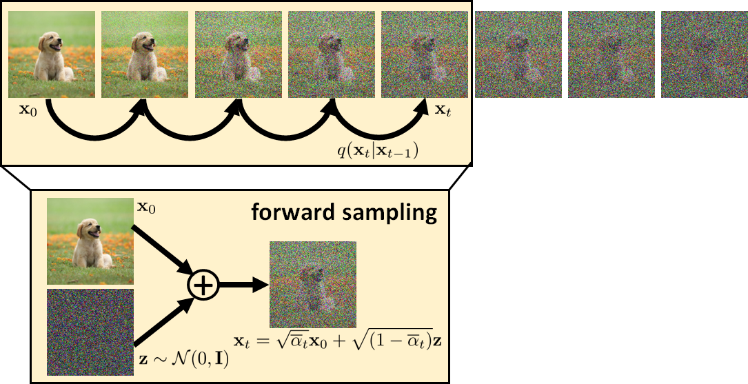
  Figure 14: Forward sampling process. The forward sampling process is originally a chain of operations. However, if we assume Gaussian, then we can simplify the sampling process as a one-step data generation.

• $\frac{1}{2\sigma_{q}^{2}(t)}\frac{(1-\alpha_{t})^{2}\overline{\alpha}_{t-1}}{(1-\overline{\alpha}_{t})^{2}}$: We do not weight the denoising loss equally for all steps. Instead, there is a scheduler to controls the relative emphasis on each denoising loss. However, for simplicity, we can drop these. It has minor impacts.

• $\sum_{t=1}^{T}$: The summation can be replaced by a uniform distribution $t\sim\text{Uniform}[1,T]$.

Training a Deniosing Diffusion Probabilistic Model. (Version: Predict image) For every image $\mathbf{x}_{0}$ in your training dataset: Repeat the following steps until convergence. • Pick a random time stamp $t\sim\text{Uniform}[1,T]$. • Draw a sample $\mathbf{x}_{t}\sim\mathcal{N}(\mathbf{x}_{t}\,|\,\sqrt{\overline{\alpha}_{t}}\mathbf{x}_{0},\;\;(1-\overline{\alpha}_{t})\mathbf{I})$, i.e., $$\mathbf{x}_{t}=\overline{\alpha}_{t}\mathbf{x}_{0}+\sqrt{(1-\overline{\alpha}_{t})}\mathbf{z},\qquad\mathbf{z}\sim\mathcal{N}(0,\mathbf{I}).$$ • Take gradient descent step on $$\nabla_{\boldsymbol{\theta}}\left\|\widehat{\mathbf{x}}_{\boldsymbol{\theta}}(\mathbf{x}_{t})-\mathbf{x}_{0}\right\|^{2}$$ You can do this in batches, just like how you train any other neural networks. Note that, here, you are training one denoising network $\widehat{\mathbf{x}}_{\boldsymbol{\theta}}$ for all noisy conditions.

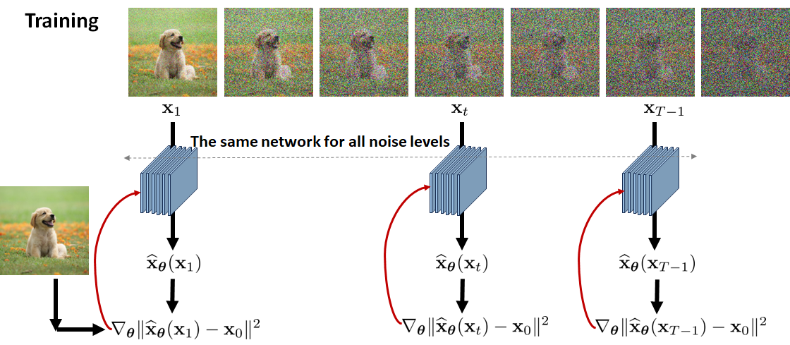
Figure 15: Training of a denoising diffusion probabilistic model. For the same neural network $\widehat{\mathbf{x}}_{\boldsymbol{\theta}}$, we send noisy inputs $\mathbf{x}_{t}$ to the network. The gradient of the loss is back-propagated to update the network. Note that the noisy images are not arbitrary. They are generated according to the forward sampling process.

Once the denoiser $\widehat{\mathbf{x}}_{\boldsymbol{\theta}}$ is trained, we can apply it to do the inference. The inference is about sampling images from the distributions $p_{\boldsymbol{\theta}}(\mathbf{x}_{t-1}|\mathbf{x}_{t})$ over the sequence of states $\mathbf{x}_{T},\mathbf{x}_{T-1},\ldots,\mathbf{x}_{1}$. Since it is the reverse diffusion process, we need to do it recursively via:

$$\mathbf{x}_{t-1}\sim p_{\boldsymbol{\theta}}(\mathbf{x}_{t-1}\,|\,\mathbf{x}_{t}) =\mathcal{N}(\mathbf{x}_{t-1}\,|\,\boldsymbol{\mu}_{\boldsymbol{\theta}}(\mathbf{x}_{t}),\sigma_{q}^{2}(t)\mathbf{I})$$

$$=\boldsymbol{\mu}_{\boldsymbol{\theta}}(\mathbf{x}_{t})+\sigma_{q}^{2}(t)\mathbf{z},\qquad\qquad\qquad\text{where}\quad\mathbf{z}\sim\mathcal{N}(0,\mathbf{I})$$

$$=\frac{(1-\overline{\alpha}_{t-1})\sqrt{\alpha_{t}}}{1-\overline{\alpha}_{t}}\mathbf{x}_{t}+\frac{(1-\alpha_{t})\sqrt{\overline{\alpha}_{t-1}}}{1-\overline{\alpha}_{t}}\widehat{\mathbf{x}}_{\boldsymbol{\theta}}(\mathbf{x}_{t})+\sigma_{q}(t)\mathbf{z}.$$

This leads to the following inferencing algorithm.

Inference on a Deniosing Diffusion Probabilistic Model. (Version: Predict image) You give us a white noise vector $\mathbf{x}_{T}\sim\mathcal{N}(0,\mathbf{I})$. • Repeat the following for $t=T,T-1,\ldots,1$. • We calculate $\widehat{\mathbf{x}}_{\boldsymbol{\theta}}(\mathbf{x}_{t})$ using our trained denoiser. • Update according to $\displaystyle\mathbf{x}_{t-1}$ $\displaystyle=\frac{(1-\overline{\alpha}_{t-1})\sqrt{\alpha_{t}}}{1-\overline{\alpha}_{t}}\mathbf{x}_{t}+\frac{(1-\alpha_{t})\sqrt{\overline{\alpha}_{t-1}}}{1-\overline{\alpha}_{t}}\widehat{\mathbf{x}}_{\boldsymbol{\theta}}(\mathbf{x}_{t})+\sigma_{q}(t)\mathbf{z},\qquad\mathbf{z}\sim\mathcal{N}(0,\mathbf{I}).$ (56)

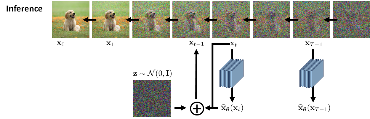
Figure 16: Inference of a denoising diffusion probabilistic model.

2.8 Derivation based on Noise Vector

If you are familiar with the denoising literature, you probably know the residue-type of algorithm that predicts the noise instead of the signal. The same spirit applies to denoising diffusion, where we can learn to predict the noise. To see why this is the case, we consider Eqn (24). If we re-arrange the terms we will obtain

$$\mathbf{x}_{t}=\sqrt{\overline{\alpha}_{t}}\mathbf{x}_{0}+\sqrt{1-\overline{\alpha}_{t}}\boldsymbol{\epsilon}_{0}$$

$$\Rightarrow\qquad \mathbf{x}_{0}=\frac{\mathbf{x}_{t}-\sqrt{1-\overline{\alpha}_{t}}\boldsymbol{\epsilon}_{0}}{\sqrt{\overline{\alpha}_{t}}}.$$

Substituting this into $\boldsymbol{\mu}_{q}(\mathbf{x}_{t},\mathbf{x}_{0})$, we can show that

$$\boldsymbol{\mu}_{q}(\mathbf{x}_{t},\mathbf{x}_{0}) =\frac{\sqrt{\alpha_{t}}(1-\overline{\alpha}_{t-1})\mathbf{x}_{t}+\sqrt{\overline{\alpha}_{t-1}}(1-\alpha_{t})\mathbf{x}_{0}}{1-\overline{\alpha}_{t}}$$

$$=\frac{\sqrt{\alpha_{t}}(1-\overline{\alpha}_{t-1})\mathbf{x}_{t}+\sqrt{\overline{\alpha}_{t-1}}(1-\alpha_{t})\cdot\frac{\mathbf{x}_{t}-\sqrt{1-\overline{\alpha}_{t}}\boldsymbol{\epsilon}_{0}}{\sqrt{\overline{\alpha}_{t}}}}{1-\overline{\alpha}_{t}}$$

$$=\text{a few more algebraic steps}$$

$$=\frac{1}{\sqrt{\alpha_{t}}}\mathbf{x}_{t}-\frac{1-\alpha_{t}}{\sqrt{1-\overline{\alpha}_{t}}\sqrt{\alpha}_{t}}\boldsymbol{\epsilon}_{0}.$$ (57)

So, if we can design our mean estimator $\boldsymbol{\mu}_{\boldsymbol{\theta}}$, we can freely choose it to match for the form:

$$\boldsymbol{\mu}_{\boldsymbol{\theta}}(\mathbf{x}_{t})=\frac{1}{\sqrt{\alpha_{t}}}\mathbf{x}_{t}-\frac{1-\alpha_{t}}{\sqrt{1-\overline{\alpha}_{t}}\sqrt{\alpha}_{t}}\widehat{\boldsymbol{\epsilon}}_{\boldsymbol{\theta}}(\mathbf{x}_{t}).$$ (58)

Substituting Eqn (57) and Eqn (58) into Eqn (50) will give us a new ELBO

$$\text{ELBO}_{\boldsymbol{\theta}}=-\sum_{t=1}^{T}\mathbb{E}_{q(\mathbf{x}_{t}|\mathbf{x}_{0})}\Big{[}\frac{1}{2\sigma_{q}^{2}(t)}\frac{(1-\alpha_{t})^{2}\overline{\alpha}_{t-1}}{(1-\overline{\alpha}_{t})^{2}}\left\|\widehat{\boldsymbol{\epsilon}}_{\boldsymbol{\theta}}(\mathbf{x}_{t})-\boldsymbol{\epsilon}_{0}\right\|^{2}\Big{]}.$$

Therefore, if you give us $\mathbf{x}_{t}$, we will return you a predicted noise $\widehat{\boldsymbol{\epsilon}}_{\boldsymbol{\theta}}(\mathbf{x}_{t})$. This will give us an alternative training scheme Training a Deniosing Diffusion Probabilistic Model (Version Predict noise). For every image $\mathbf{x}_{0}$ in your training dataset: Repeat the following steps until convergence. • Pick a random time stamp $t\sim\text{Uniform}[1,T]$. • Draw a sample $\mathbf{x}_{t}\sim\mathcal{N}(\mathbf{x}_{t}\,|\,\sqrt{\overline{\alpha}_{t}}\mathbf{x}_{0},\;\;(1-\overline{\alpha}_{t})\mathbf{I})$, i.e., $$\mathbf{x}_{t}=\sqrt{\overline{\alpha}_{t}}\mathbf{x}_{0}+\sqrt{(1-\overline{\alpha}_{t})}\mathbf{z},\qquad\mathbf{z}\sim\mathcal{N}(0,\mathbf{I}).$$ • Take gradient descent step on $$\nabla_{\boldsymbol{\theta}}\left\|{\color[rgb]{0,0,1}\widehat{\boldsymbol{\epsilon}}_{\boldsymbol{\theta}}(\mathbf{x}_{t})}-{\color[rgb]{0,0,1}\boldsymbol{\epsilon}_{0}}\right\|^{2}$$ Consequently, the inference step can be derived through

$$\mathbf{x}_{t-1}\sim p_{\boldsymbol{\theta}}(\mathbf{x}_{t-1}\,|\,\mathbf{x}_{t}) =\mathcal{N}(\mathbf{x}_{t-1}\,|\,\boldsymbol{\mu}_{\boldsymbol{\theta}}(\mathbf{x}_{t}),\sigma_{q}^{2}(t)\mathbf{I})$$

$$=\boldsymbol{\mu}_{\boldsymbol{\theta}}(\mathbf{x}_{t})+\sigma_{q}^{2}(t)\mathbf{z}$$

$$=\frac{1}{\sqrt{\alpha_{t}}}\mathbf{x}_{t}-\frac{1-\alpha_{t}}{\sqrt{1-\overline{\alpha}_{t}}\sqrt{\alpha}_{t}}\widehat{\boldsymbol{\epsilon}}_{\boldsymbol{\theta}}(\mathbf{x}_{t})+\sigma_{q}(t)\mathbf{z}$$

$$=\frac{1}{\sqrt{\alpha_{t}}}\left(\mathbf{x}_{t}-\frac{1-\alpha_{t}}{\sqrt{1-\overline{\alpha}_{t}}}\widehat{\boldsymbol{\epsilon}}_{\boldsymbol{\theta}}(\mathbf{x}_{t})\right)+\sigma_{q}(t)\mathbf{z}$$

Summarizing it here, we have Inference on a Deniosing Diffusion Probabilistic Model. (Version Predict noise) You give us a white noise vector $\mathbf{x}_{T}\sim\mathcal{N}(0,\mathbf{I})$. • Repeat the following for $t=T,T-1,\ldots,1$. • We calculate $\widehat{\mathbf{x}}_{\boldsymbol{\theta}}(\mathbf{x}_{t})$ using our trained denoiser. • Update according to $\displaystyle\mathbf{x}_{t-1}$ $\displaystyle=\frac{1}{\sqrt{\alpha_{t}}}\left(\mathbf{x}_{t}-\frac{1-\alpha_{t}}{\sqrt{1-\overline{\alpha}_{t}}}\widehat{\boldsymbol{\epsilon}}_{\boldsymbol{\theta}}(\mathbf{x}_{t})\right)+\sigma_{q}(t)\mathbf{z},\qquad\mathbf{z}\sim\mathcal{N}(0,\mathbf{I}).$

2.9 Inversion by Direct Denoising (InDI)

If we look at the DDPM equation, we will see that the update Eqn (56) takes the following form:

$$\mathbf{x}_{t-1}=\Big{(}\text{something}\Big{)}\cdot\mathbf{x}_{t}+\Big{(}\text{something else}\Big{)}\cdot\text{denoise}(\mathbf{x}_{t})+\text{noise}.$$ (59)

In other words, the $(t-1)$-th estimate is a linear combination of three terms: the current estimate $\mathbf{x}_{t}$, the denoised version $\text{denoise}(\mathbf{x}_{t})$ and a noise term. The current estimate and the noise term are easy to understand. But what is “denoise”? An interesting paper by Delbracio and Milanfar [6] looked at the generative diffusion models from a pure denoising perspective. As it turns out, this surprisingly simple perspective is consistent with the other more advanced diffusion models in some good ways.

What is $\text{denoise}(\mathbf{x}_{t})$? Denoising is a generic procedure that removes noise from a noisy image. In the good old days of statistical signal processing, a standard textbook problem is to derive the optimal denoiser for white noise. Given the observation model

$$\mathbf{y}=\mathbf{x}+\boldsymbol{\epsilon},\qquad\text{where}\;\;\boldsymbol{\epsilon}\sim\mathcal{N}(0,\mathbf{I}),$$

can you construct an estimator $g(\cdot)$ such that the mean squared error is minimized?

We shall skip the derivation of the solution to this classical problem because you can find it in any probability textbook, e.g., [7, Chapter 8]. The solution is

$$\text{denoise}(\mathbf{y}) =\mathop{\underset{g}{\mbox{argmin}}}\;\;\mathbb{E}_{\mathbf{x},\mathbf{y}}[\|g(\mathbf{y})-\mathbf{x}\|^{2}]$$

$$=\text{some magical step}$$

$$=\mathbb{E}[\mathbf{x}|\mathbf{y}].$$ (60)

So, going back to our problem: If we assume that

$$\mathbf{x}_{t}=\mathbf{x}_{t-1}+\boldsymbol{\epsilon}_{t-1},\qquad\text{where}\;\;\boldsymbol{\epsilon}_{t-1}\sim\mathcal{N}(0,\mathbf{I}),$$

then clearly the denoiser is the conditional expectation of the posterior distribution:

$$\text{denoise}(\mathbf{x}_{t})=\mathbb{E}[\mathbf{x}_{t-1}|\mathbf{x}_{t}].$$ (61)

Thus, if we are given the distribution $p_{\boldsymbol{\theta}}(\mathbf{x}_{t-1}|\mathbf{x}_{t})$, then the optimal denoiser is just the conditional expectation of this distribution. Such a denoiser is called the minimum mean squared error (MMSE) denoiser. MMSE denoiser is not the “best” denoiser; It is only the optimal denoiser with respect to the mean squared error. Since mean squared error is never a good metric for image quality, minimizing the MSE will not necessarily give us a better image. Nevertheless, people like MMSE denoisers because they are easy to derive.

Incremental Denoising Steps. If you understand that an MMSE denoiser is equivalent to the conditional expectation of the posterior distribution, you will appreciate the incremental denoising. Here is how it works. Suppose that we have a clean image $\mathbf{x}_{0}$ and a noise image $\mathbf{y}$. Our goal is to form a linear combination of $\mathbf{x}_{0}$ and $\mathbf{y}$ via a simple equation

$$\mathbf{x}_{t}=(1-t)\mathbf{x}_{0}+t\mathbf{y},\qquad 0\leq t\leq 1.$$ (62)

Now, consider a small step $\tau$ previous to time $t$. The following result, showed by [6], provides some useful utilities: Let $0\leq\tau<t\leq 1$ , and suppose that $\mathbf{x}_{t}=(1-t)\mathbf{x}_{0}+t\mathbf{y}$, then it holds that $$\mathbb{E}[\mathbf{x}_{t-\tau}|\mathbf{x}_{t}]=\left(1-\frac{\tau}{t}\right)\underset{\text{current estimate}}{\underbrace{\mathbf{x}_{t}}}\qquad+\qquad\frac{\tau}{t}\;\;\;\;\underset{\text{denoised}}{\underbrace{\mathbb{E}[\mathbf{x}_{0}|\mathbf{x}_{t}]}}.$$ (63) If we define $\widehat{\mathbf{x}}_{t-\tau}$ as the left hand side, replace $\mathbf{x}_{t}$ by $\widehat{\mathbf{x}}_{t}$, and write $\mathbb{E}[\mathbf{x}_{0}|\mathbf{x}_{t}]$ as $\text{denoise}(\widehat{\mathbf{x}}_{t})$, then the above equation will become

$$\widehat{\mathbf{x}}_{t-\tau}=\left(1-\frac{\tau}{t}\right)\cdot\widehat{\mathbf{x}}_{t}+\frac{\tau}{t}\text{denoise}(\widehat{\mathbf{x}}_{t}),$$ (64)

where $\tau$ is a small step in time.

Eqn (64) gives us an inference step. If you tell us the denoiser and suppose that you start with a noisy image $\mathbf{y}$, then we can iteratively apply Eqn (64) to retrieve the images $\widehat{\mathbf{x}}_{t-1}$, $\widehat{\mathbf{x}}_{t-2}$, …, $\widehat{\mathbf{x}}_{0}$.

Training. The training of the iterative scheme requires a denoiser that generates $\text{denoise}(\mathbf{x}_{t})$. To this end, we can train a neural network $\text{denoise}_{\boldsymbol{\theta}}$ (where $\boldsymbol{\theta}$ denotes the network weight):

$$\mathop{\underset{\boldsymbol{\theta}}{\mathrm{minimize}}}\;\;\mathbb{E}_{\mathbf{x},\mathbf{y}}\mathbb{E}_{t\sim\text{uniform}}\Big{[}\|\text{denoise}_{\boldsymbol{\theta}}(\mathbf{x}_{t})-\mathbf{x}\|^{2}\Big{]}.$$ (65)

Here, the distribution “$t\sim\text{uniform}$” specifies that the time step $t$ is drawn uniformly from a given distribution. Therefore, we are training one denoiser for all time steps $t$. The expectation $(\mathbf{x},\mathbf{y})$ is generally fulfilled when you use a pair of noisy and clean images from the training dataset. After training, we can perform the incremental update via Eqn (64).

Connection with Denoising Score-Matching. Although we have not yet discussed score-matching (which will be presented in the next Section), an interesting fact about the above iterative denoising procedure is that it is related to denoising score-matching. At the high level, we can rewrite the iteration as

$$\mathbf{x}_{t-\tau} =\left(1-\frac{\tau}{t}\right)\cdot\mathbf{x}_{t}+\frac{\tau}{t}\text{denoise}(\mathbf{x}_{t})$$

$$\Rightarrow\qquad \mathbf{x}_{t-\tau}-\mathbf{x}_{t} =-\frac{\tau}{t}\mathbf{x}_{t}+\frac{\tau}{t}\text{denoise}(\mathbf{x}_{t})$$

$$\Rightarrow\qquad \frac{\mathbf{x}_{t}-\mathbf{x}_{t-\tau}}{\tau} =\frac{\mathbf{x}_{t}-\text{denoise}(\mathbf{x}_{t})}{t}$$

$$\Rightarrow\qquad \frac{d\mathbf{x}_{t}}{dt}=\lim_{\tau\rightarrow 0}\frac{\mathbf{x}_{t}-\mathbf{x}_{t-\tau}}{\tau} =\frac{\mathbf{x}_{t}-\text{denoise}(\mathbf{x}_{t})}{t}$$

This is an ordinary differential equation (ODE). If we let $\mathbf{x}_{t}=\mathbf{x}+t\boldsymbol{\epsilon}$ so that the noise level in $\mathbf{x}_{t}$ is $\sigma_{t}^{2}=t^{2}\sigma^{2}$, then we can use several results in the literature to show that

$$\frac{d\mathbf{x}_{t}}{dt} =-\frac{1}{2}\frac{d(\sigma_{t}^{2})}{dt}\nabla_{\mathbf{x}_{t}}\log p_{t}(\mathbf{x}_{t}) (\text{ODE defined by Song et al. \cite[cite]{[\@@bibref{}{Song_2021_SGM}{}{}]}})$$

$$=-t\sigma^{2}\nabla_{\mathbf{x}_{t}}\log p_{t}(\mathbf{x}_{t}) (\sigma_{t}=t\sigma)$$

$$\approx-t\sigma^{2}\frac{\mathbf{x}-\text{denoise}(\mathbf{x}_{t})}{t^{2}\sigma^{2}} (\text{Approximation proposed by Vincent \cite[cite]{[\@@bibref{}{Vincent_2011_DSM}{}{}]}})$$

$$=\frac{\mathbf{x}_{t}-\text{denoise}(\mathbf{x}_{t})}{t}.$$

Therefore, the incremental denoising iteration is equivalent to the denoising score-matching, at least in the limiting case determined by the ODE.

Adding Stochastic Steps. The above incremental denoising iteration can be equipped with stochastic perturbation. For the inference step, we can define a sequence of noise levels $\{\sigma_{t}\;|\;0\leq t\leq 1\}$, and define

$$\widehat{\mathbf{x}}_{t-\tau}=\left(1-\frac{\tau}{t}\right)\cdot\widehat{\mathbf{x}}_{t}+\frac{\tau}{t}\text{denoise}(\widehat{\mathbf{x}}_{t})+(t-\tau)\sqrt{\sigma_{t-\tau}^{2}-\sigma_{t}^{2}}\boldsymbol{\epsilon},\qquad\boldsymbol{\epsilon}\sim\mathcal{N}(0,\mathbf{I}).$$ (66)

As or training, one can train a denoiser via

$$\mathop{\underset{\boldsymbol{\theta}}{\mathrm{minimize}}}\;\;\mathbb{E}_{(\mathbf{x},\mathbf{y})}\mathbb{E}_{t\sim\text{uniform}}\mathbb{E}_{\boldsymbol{\epsilon}}\left[\|\text{denoise}(\mathbf{x}_{t})-\mathbf{x}\|^{2}\right],$$ (67)

where $\mathbf{x}_{t}=(1-t)\mathbf{x}+t\mathbf{y}+\sqrt{t}\sigma_{t}\boldsymbol{\epsilon}$.

Congratulations! We are done. This is all about DDPM.

The literature of DDPM is quickly exploding. The original paper by Sohl-Dickstein et al. [10] and Ho et al. [4] are the must-reads to understand the topic. For a more “user-friendly” version, we found that the tutorial by Luo very useful [11]. Some follow up works are highly cited, including the denoising diffusion implicit models by Song et al. [12]. In terms of application, people have been using DDPM for various image synthesis applications, e.g., [13, 14].

3 Score-Matching Langevin Dynamics (SMLD)

Score-based generative models [8] are alternative approaches to generate data from a desired distribution. There are several core ingredients: the Langevin dynamics, the (Stein) score function, and the score-matching loss. In this section, we will look at these topics one by one.

3.1 Langevin Dynamics

An interesting starting point of our discussion is the Langevin dynamics. It is a very physics topic that will appear to have nothing to do with generative models. But please don’t worry. They are related, in fact, in a good way.

Instead of telling you the physics right a way, let’s talk about how Langevin dynamics can be used to draw samples from a distribution. Imagine that we are given a distribution $p(\mathbf{x})$ and suppose that we want to draw samples from $p(\mathbf{x})$. Langevin dynamics is an iterative procedure that allows us to draw samples according to the following equation. The Langevin dynamics for sampling from a known distribution $p(\mathbf{x})$ is an iterative procedure for $t=1,\ldots,T$: $$\mathbf{x}_{t+1}=\mathbf{x}_{t}+\tau\nabla_{\mathbf{x}}\log p(\mathbf{x}_{t})+\sqrt{2\tau}\mathbf{z},\qquad\mathbf{z}\sim\mathcal{N}(0,\mathbf{I}),$$ (68) where $\tau$ is the step size which users can control, and $\mathbf{x}_{0}$ is white noise.

You may wonder, what on the Earth is this mysterious equation about?! Here is the short and quick answer. If you ignore the noise term $\sqrt{2\tau}\mathbf{z}$ at the end, the Langevin dynamics equation in Eqn (68) is literally gradient descent. The descent direction $\nabla_{\mathbf{x}}\log p(\mathbf{x})$ is carefully chosen that $\mathbf{x}_{t}$ will converge to the distribution $p(\mathbf{x})$. If you watch any YouTube videos mumbling Langevin dynamics equations for 10 minutes without explaining what it is, you can gently tell them the following: Without the noise term, Langevin dynamics is gradient descent.

Consider a distribution $p(\mathbf{x})$. The shape of this distribution is defined and is fixed as soon as the model parameters are defined. For example, if you choose a Gaussian, the shape and location of the Gaussian is fixed once you specify the mean and the variance. The value $p(\mathbf{x})$ is nothing but the probability density evaluated at a data point $\mathbf{x}$. Therefore, going from one $\mathbf{x}$ to another $\mathbf{x}^{\prime}$, we are just moving from one value $p(\mathbf{x})$ to a different value $p(\mathbf{x}^{\prime})$. The underlying shape of the Gaussian is not changed.

Suppose that we start with some arbitrary location in $\mathbb{R}^{d}$. We want to move it to (one of) the peak(s) of the distribution. The peak is a special place because it is where the probability is the highest. So, if we say that a sample $\mathbf{x}$ is drawn from a distribution $p(\mathbf{x})$, certainly the “optimal” location for $\mathbf{x}$ is where $p(\mathbf{x})$ is maximized. If $p(\mathbf{x})$ has multiple local minima, any one of them would be fine. So, naturally, the goal of sampling is equivalent to solving the optimization

$$\mathbf{x}^{*}=\mathop{\underset{\mathbf{x}}{\mbox{argmax}}}\;\;\log p(\mathbf{x}).$$

We emphasize again that this is not maximum likelihood estimation. In maximum likelihood, the data point $\mathbf{x}$ is fixed but the model parameters are changing. Here, the model parameters are fixed but the data point is changing. The table below summarizes the difference.

Problem	Sampling	Maximum Likelihood
Optimization target	A sample $\mathbf{x}$	Model parameter $\boldsymbol{\theta}$
Formulation	$\mathbf{x}^{*}=\mathop{\underset{\mathbf{x}}{\mbox{argmax}}}\;\;\log p(\mathbf{x};\boldsymbol{\theta})$	$\boldsymbol{\theta}^{*}=\mathop{\underset{\boldsymbol{\theta}}{\mbox{argmax}}}\;\;\log p(\mathbf{x};\boldsymbol{\theta})$

The optimization can be solved in many ways. The cheapest way is, of course, gradient descent. For $\log p(\mathbf{x})$, we see that the gradient descent step is

$$\mathbf{x}_{t+1}=\mathbf{x}_{t}+\tau\nabla_{\mathbf{x}}\log p(\mathbf{x}_{t}),$$

where $\nabla_{\mathbf{x}}\log p(\mathbf{x}_{t})$ denotes the gradient of $\log p(\mathbf{x})$ evaluated at $\mathbf{x}_{t}$, and $\tau$ is the step size. Here we use “$+$” instead of the typical “$-$” because we are solving a maximization problem.

Example. Consider a Gaussian distribution $p(x)=\mathcal{N}(x\,|\,\mu,\sigma^{2})$, we can easily show that the Langevin dynamics equation is $\displaystyle x_{t+1}$ $\displaystyle=x_{t}+\tau\cdot\nabla_{x}\log\left\{\frac{1}{\sqrt{2\pi\sigma^{2}}}e^{-\frac{(x-\mu)^{2}}{2\sigma^{2}}}\right\}+\sqrt{2\tau}z$ $\displaystyle=x_{t}-\tau\cdot\frac{x_{t}-\mu}{\sigma^{2}}+\sqrt{2\tau}z,$ $\displaystyle\qquad z\sim\mathcal{N}(0,1)$

Example. Consider a Gaussian mixture $p(x)=\pi_{1}\mathcal{N}(x\,|\,\mu_{1},\sigma_{1}^{2})+\pi_{2}\mathcal{N}(x\,|\,\mu_{2},\sigma_{2}^{2})$. We can numerically calculate $\nabla_{x}\log p(x)$. For demonstration, we choose $\pi_{1}=0.6$. $\mu_{1}=2$, $\sigma_{1}=0.5$, $\pi_{2}=0.4$, $\mu_{2}=-2$, $\sigma_{2}=0.2$. We initialize $x_{0}=0$. We choose $\tau=0.05$. We run the above gradient descent iteration for $T=500$ times, and we plot the trajectory of the values $p(x_{t})$ for $t=1,\ldots,T$. As we can see in the figure below, the sequence $\{x_{1},x_{2},\ldots,x_{T}\}$ simply follows the shape of the Gaussian and climb to one of the peaks. What is more interesting is when we add the noise term. Instead of landing at the peak, the sequence $x_{t}$ move around the peak and finishes somewhere near the peak. The closer we are to the peak, the higher probability we will stop there. $\mathbf{x}_{t+1}=\mathbf{x}_{t}+\tau\nabla_{\mathbf{x}}\log p(\mathbf{x}_{t})$ $\mathbf{x}_{t+1}=\mathbf{x}_{t}+\tau\nabla_{\mathbf{x}}\log p(\mathbf{x}_{t})+\sqrt{2\tau}\mathbf{z}$

Figure 17 shows an interesting description of the sample trajectory. Starting with an arbitrary location, the data point $\mathbf{x}_{t}$ will do a random walk according to the Langevin dynamics equation. The direction of the random walk is not completely arbitrary. There is a certain amount of pre-defined drift while at every step there is some level of randomness. The drift is determined by $\nabla_{\mathbf{x}}\log p(\mathbf{x})$ where as the randomness comes from $\mathbf{z}$.

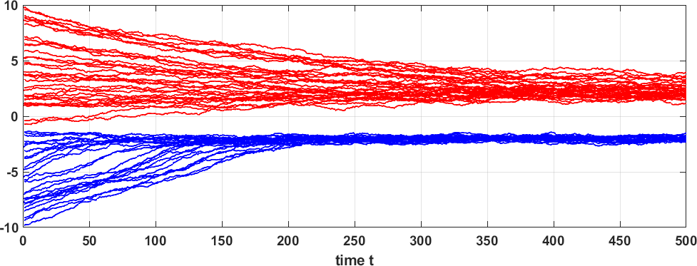
Figure 17: Trajectory of sample evolutions using the Langevin dynamics. We colored the two modes of the Gaussian mixture in different colors for better visualization. The setting here is identical to the example above, except that the step size is $\tau=0.001$.

As we can see from the example above, the addition of the noise term actually changes the gradient descent to stochastic gradient descent. Instead of shooting for the deterministic optimum, the stochastic gradient descent climbs up the hill randomly. Since we use a constant step size $\sqrt{2\tau}$, the final solution will just oscillate around the peak. So, we can summarize Langevin dynamics equation as Langevin dynamics is stochastic gradient descent. But why do we want to do stochastic gradient descent instead of gradient descent? The key is that we are not interested in solving the optimization problem. Instead, we are more interested in sampling from a distribution. By introducing the random noise to the gradient descent step, we randomly pick a sample that is following the objective function’s trajectory while not staying at where it is. If we are closer to the peak, we will move left and right slightly. If we are far from the peak, the gradient direction will pull us towards the peak. If the curvature around the peak is sharp, we will concentrate most of the steady state points $\mathbf{x}_{T}$ there. If the curvature around the peak is flat, we will spread around. Therefore, by repeatedly initialize the stochastic gradient descent algorithm at a uniformly distributed location, we will eventually collect samples that will follow the distribution we designate.

Example. Consider a Gaussian mixture $p(x)=\pi_{1}\mathcal{N}(x\,|\,\mu_{1},\sigma_{1}^{2})+\pi_{2}\mathcal{N}(x\,|\,\mu_{2},\sigma_{2}^{2})$. We can numerically calculate $\nabla_{x}\log p(x)$. For demonstration, we choose $\pi_{1}=0.6$. $\mu_{1}=2$, $\sigma_{1}=0.5$, $\pi_{2}=0.4$, $\mu_{2}=-2$, $\sigma_{2}=0.2$. Suppose we initialize $M=10000$ uniformly distributed samples $x_{0}\sim\text{Uniform}[-3,3]$. We run Langevin updates for $t=100$ steps. The histograms of generated samples are shown in the figures below.

Remark: Origin of Langevin Dynamics. The name Langevin dynamics of course does not originate from our “hacking” point of view. It starts with physics. Consider the basic Newton equation which relates force $\mathbf{F}$ with mass $m$ and velocity $\mathbf{v}(t)$. Newton’s second law says that $$\underset{\text{force}}{\underbrace{\mathbf{F}}}=\underset{\text{mass}}{\underbrace{m}}\cdot\underset{\text{acceleration}}{\underbrace{\frac{d\mathbf{v}(t)}{dt}}}.$$ (69) Given force $\mathbf{F}$, we also know that it is related to the potential energy $U(\mathbf{x})$ via $$\underset{\text{force}}{\underbrace{\mathbf{F}}}=\nabla_{\mathbf{x}}\underset{\text{energy}}{\underbrace{U(\mathbf{x})}}.$$ (70) The randomness of Langevin dynamics comes from Brownian motion. Imagine that we have a bag of molecules moving around. Their motion can be described according to the Brownian motion model: $$\frac{d\mathbf{v}(t)}{dt}=-\frac{\lambda}{m}\mathbf{v}(t)+\frac{1}{m}\boldsymbol{\eta},\qquad\text{where}\;\;\boldsymbol{\eta}\sim\mathcal{N}(0,\sigma^{2}\mathbf{I}).$$ (71) Therefore, substituting Eqn (71) into Eqn (69), and equating it with Eqn (70), we have $\displaystyle-\nabla_{\mathbf{x}}U(\mathbf{x})=-\lambda\mathbf{v}(t)+\boldsymbol{\eta}\quad\Rightarrow\quad\mathbf{v}(t)=-\frac{1}{\lambda}\nabla_{\mathbf{x}}U(\mathbf{x})+\frac{1}{\lambda}\boldsymbol{\eta}.$ This can be equivalently written as $$\frac{d\mathbf{x}}{dt}=-\frac{1}{\lambda}\nabla_{\mathbf{x}}U(\mathbf{x})+\frac{\sigma}{\lambda}\mathbf{z},\qquad\text{where}\;\;\mathbf{z}\sim\mathcal{N}(0,\mathbf{I}).$$ (72) If we let $\tau=\frac{dt}{\lambda}$ and discretize the above differential equation, we will obtain $$\mathbf{x}_{t+1}=\mathbf{x}_{t}-\tau\nabla_{\mathbf{x}}U(\mathbf{x}_{t})+\sigma\tau\mathbf{z}_{t}.$$ (73) So it remains to identify the energy potential. A very reasonable (and lazy) choice for our probability distribution function $p(\mathbf{x})$ is the Boltzmann distribution with the form $\displaystyle p(\mathbf{x})=\frac{1}{Z}\exp\left\{-U(\mathbf{x})\right\}.$ Therefore, it follows immediately that $$\nabla_{\mathbf{x}}\log p(\mathbf{x})=\nabla_{\mathbf{x}}\Big{\{}-U(\mathbf{x})-\log Z\Big{\}}=-\nabla_{\mathbf{x}}U(\mathbf{x}).$$ (74) Substituting Eqn (74) into Eqn (73) would yield $\mathbf{x}_{t+1}=\mathbf{x}_{t}+\tau\nabla_{\mathbf{x}}\log p(\mathbf{x})+\sigma\tau\mathbf{z}$. Finally, if we choose $\sigma=\sqrt{2/\tau}$ (for no particular reason), we will obtain $$\mathbf{x}_{t+1}=\mathbf{x}_{t}+\tau\nabla_{\mathbf{x}}\log p(\mathbf{x}_{t})+\sqrt{2\tau}\mathbf{z}_{t}.$$ (75)

3.2 (Stein’s) Score Function

The second component of the Langevin dynamics equation is the gradient $\nabla_{\mathbf{x}}\log p(\mathbf{x})$. It has a formal name known as the Stein’s score function, denoted by

$$\mathbf{s}_{\boldsymbol{\theta}}(\mathbf{x})\overset{\text{def}}{=}\nabla_{\mathbf{x}}\log p_{\boldsymbol{\theta}}(\mathbf{x}).$$ (76)

We should be careful not to confuse Stein’s score function with the ordinary score function which is defined as

$$\mathbf{s}_{\mathbf{x}}(\boldsymbol{\theta})\overset{\text{def}}{=}\nabla_{\boldsymbol{\theta}}\log p_{\boldsymbol{\theta}}(\mathbf{x}).$$ (77)

The ordinary score function is the gradient (wrt $\boldsymbol{\theta}$) of the log-likelihood. In contrast, the Stein’s score function is the gradient wrt the data point $\mathbf{x}$. Maximum likelihood estimation uses the ordinary score function, whereas Langevin dynamics uses Stein’s score function. However, since most people in the diffusion literature calls Stein’s score function as the score function, we follow this culture. The “score function” in Langevin dynamics is more accurately known as the Stein’s score function.

The way to understand the score function is to remember that it is the gradient with respect to the data $\mathbf{x}$. For any high-dimensional distribution $p(\mathbf{x})$, the gradient will give us vector field

$$\nabla_{\mathbf{x}}\log p(\mathbf{x})=\text{a vector field}=\left[\frac{\partial\log p(\mathbf{x})}{\partial x},\;\;\frac{\partial\log p(\mathbf{x})}{\partial y}\right]^{T}$$ (78)

Let’s consider two examples. Example. If $p(x)$ is a Gaussian with $p(x)=\frac{1}{\sqrt{2\pi\sigma^{2}}}e^{-\frac{(x-\mu)^{2}}{2\sigma^{2}}}$, then $$s(x)=\nabla_{x}\log p(x)=-\frac{(x-\mu)}{\sigma^{2}}.$$

Example. If $p(x)$ is a Gaussian mixture with $p(x)=\sum_{i=1}^{N}\pi_{i}\frac{1}{\sqrt{2\pi\sigma_{i}^{2}}}e^{-\frac{(x-\mu_{i})^{2}}{2\sigma_{i}^{2}}}$, then $$s(x)=\nabla_{x}\log p(x)=-\frac{\sum_{j=1}^{N}\pi_{j}\frac{1}{\sqrt{2\pi\sigma_{j}^{2}}}e^{-\frac{(x-\mu_{j})^{2}}{2\sigma_{j}^{2}}}\frac{(x-\mu_{j})}{\sigma_{j}^{2}}}{\sum_{i=1}^{N}\pi_{i}\frac{1}{\sqrt{2\pi\sigma_{i}^{2}}}e^{-\frac{(x-\mu_{i})^{2}}{2\sigma_{i}^{2}}}}.$$

The probability density function and the corresponding score function of the above two examples are shown in Figure 18.

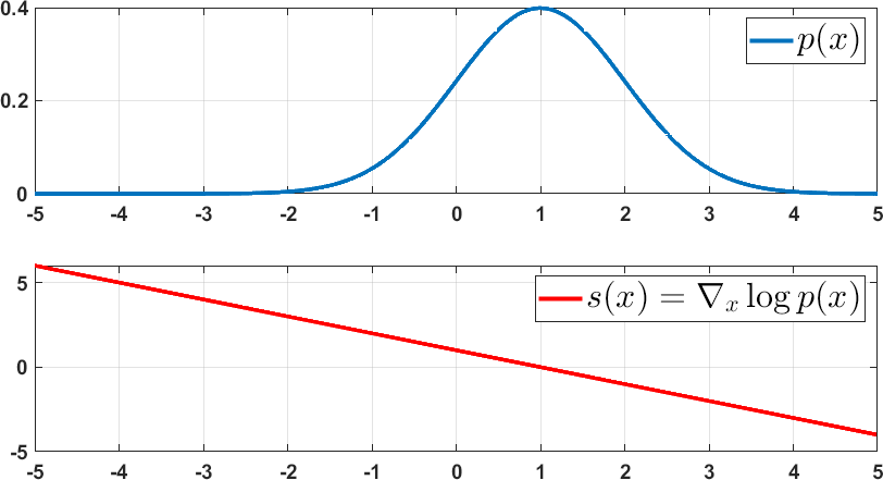
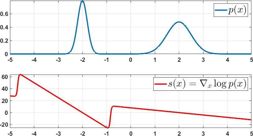
(a) $\mathcal{N}(1,1)$	(b) $0.6\mathcal{N}(2,0.5^{2})+0.4\mathcal{N}(-2,0.2^{2})$

Figure 18: Examples of score functions

Geometric Interpretations of the Score Function.

• The magnitude of the vectors are the strongest at places where the change of $\log p(\mathbf{x})$ is the biggest. Therefore, in regions where $\log p(\mathbf{x})$ is close to the peak will be mostly very weak gradient.

• The vector field indicates how a data point should travel in the contour map. In Figure 19 we show the contour map of a Gaussian mixture (with two Gaussians). We draw arrows to indicate the vector field. Now if we consider a data point living the space, the Langevin dynamics equation will basically move the data points along the direction pointed by the vector field towards the basin.

• In physics, the score function is equivalent to the “drift”. This name suggests how the diffusion particles should flow to the lowest energy state.

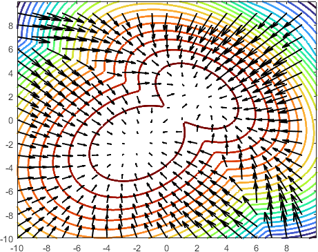
(a) vector field of $\nabla_{\mathbf{x}}\log p(\mathbf{x})$	(b) $\mathbf{x}_{t}$ trajectory

Figure 19: The contour map of the score function, and the corresponding trajectory of two samples.

3.3 Score Matching Techniques

The most difficult question in Langevin dynamics is how to obtain $\nabla_{\mathbf{x}}p(\mathbf{x})$ because we have no access to $p(\mathbf{x})$. Let’s recall the definition of the (Stein’s) score function

$$\mathbf{s}_{\boldsymbol{\theta}}(\mathbf{x})\overset{\text{def}}{=}\nabla_{\mathbf{x}}p(\mathbf{x}),$$ (79)

where we put a subscript $\boldsymbol{\theta}$ to denote that $\mathbf{s}_{\boldsymbol{\theta}}$ will be implemented via a network. Since the right hand side of the above equation is not known, we need some cheap and dirty ways to approximate it. In this section, we briefly discuss two approximation.

Explicit Score-Matching. Suppose that we are given a dataset $\mathcal{X}=\{\mathbf{x}_{1},\ldots,\mathbf{x}_{M}\}$. The solution people came up with is to consider the classical kernel density estimation by defining a distribution

$$q(\mathbf{x})=\frac{1}{M}\sum_{m=1}^{M}\frac{1}{h}K\left(\frac{\mathbf{x}-\mathbf{x}_{m}}{h}\right),$$ (80)

where $h$ is just some hyperparameter for the kernel function $K(\cdot)$, and $\mathbf{x}_{m}$ is the $m$-th sample in the training set. Figure 20 illustrates the idea of kernel density estimation. In the cartoon figure shown on the left, we show multiple kernels $K(\cdot)$ centered at different data points $\mathbf{x}_{m}$. The sum of all these individual kernels gives us the overall kernel density estimate $q(\mathbf{x})$. On the right hand side we show a real histogram and the corresponding kernel density estimate. We remark that $q(\mathbf{x})$ is at best an approximation to the true data distribution $p(\mathbf{x})$ which is never known.

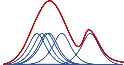
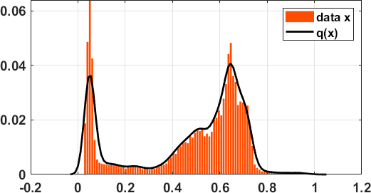
Figure 20: Illustration of kernel density estimation.

Since $q(\mathbf{x})$ is an approximation to $p(\mathbf{x})$ which is never accessible, we can learn $\mathbf{s}_{\boldsymbol{\theta}}(\mathbf{x})$ based on $q(\mathbf{x})$. This leads to the following definition of the a loss function which can be used to train a network. The explicit score matching loss is $$J_{\text{ESM}}(\boldsymbol{\theta})\overset{\text{def}}{=}\mathbb{E}_{q(\mathbf{x})}\|\mathbf{s}_{\boldsymbol{\theta}}(\mathbf{x})-\nabla_{\mathbf{x}}\log q(\mathbf{x})\|^{2}$$ (81) By substituting the kernel density estimation, we can show that the loss is

$$J_{\text{ESM}}(\boldsymbol{\theta}) \overset{\text{def}}{=}\mathbb{E}_{q(\mathbf{x})}\|\mathbf{s}_{\boldsymbol{\theta}}(\mathbf{x})-\nabla_{\mathbf{x}}\log q(\mathbf{x})\|^{2}$$

$$=\int\|\mathbf{s}_{\boldsymbol{\theta}}(\mathbf{x})-\nabla_{\mathbf{x}}\log q(\mathbf{x})\|^{2}\left[\frac{1}{M}\sum_{m=1}^{M}\frac{1}{h}K\left(\frac{\mathbf{x}-\mathbf{x}_{m}}{h}\right)\right]d\mathbf{x}$$

$$=\frac{1}{M}\sum_{m=1}^{M}\int\|\mathbf{s}_{\boldsymbol{\theta}}(\mathbf{x})-\nabla_{\mathbf{x}}\log q(\mathbf{x})\|^{2}\frac{1}{h}K\left(\frac{\mathbf{x}-\mathbf{x}_{m}}{h}\right)d\mathbf{x}.$$ (82)

So, we have derived a loss function that can be used to train the network. Once we train the network $\mathbf{s}_{\boldsymbol{\theta}}$, we can replace it in the Langevin dynamics equation to obtain the recursion:

$$\mathbf{x}_{t+1}=\mathbf{x}_{t}+\tau\mathbf{s}_{\boldsymbol{\theta}}(\mathbf{x}_{t})+\sqrt{2\tau}\mathbf{z}.$$ (83)

The issue of explicit score matching is that the kernel density estimation is a fairly poor non-parameter estimation of the true distribution. Especially when we have limited number of samples and the samples live in a high dimensional space, the kernel density estimation performance can be poor.

Denoising Score Matching. Given the potential drawbacks of explicit score matching, we now introduce a more popular score matching known as the denoising score matching (DSM). In DSM, the loss function is defined as follows.

$$J_{\text{DSM}}(\boldsymbol{\theta})\overset{\text{def}}{=}\mathbb{E}_{q(\mathbf{x},\mathbf{x}^{\prime})}\left[\frac{1}{2}\left\|\mathbf{s}_{\boldsymbol{\theta}}(\mathbf{x})-\nabla_{\mathbf{x}}q(\mathbf{x}|\mathbf{x}^{\prime})\right\|^{2}\right]$$ (84)

The key difference here is that we replace the distribution $q(\mathbf{x})$ by a conditional distribution $q(\mathbf{x}|\mathbf{x}^{\prime})$. The former requires an approximation, e.g., via kernel density estimation, whereas the latter does not. Here is an example.

In the special case where $q(\mathbf{x}|\mathbf{x}^{\prime})=\mathcal{N}(\mathbf{x}\;|\;\mathbf{x}^{\prime},\sigma^{2})$, we can let $\mathbf{x}=\mathbf{x}^{\prime}+\sigma\mathbf{z}$. This will give us

$$\nabla_{\mathbf{x}}\log q(\mathbf{x}|\mathbf{x}^{\prime}) =\nabla_{\mathbf{x}}\log\frac{1}{(\sqrt{2\pi\sigma^{2}})^{d}}\exp\left\{-\frac{\|\mathbf{x}-\mathbf{x}^{\prime}\|^{2}}{2\sigma^{2}}\right\}$$

$$=\nabla_{\mathbf{x}}\left\{-\frac{\|\mathbf{x}-\mathbf{x}^{\prime}\|^{2}}{2\sigma^{2}}-\log(\sqrt{2\pi\sigma^{2}})^{d}\right\}$$

$$=-\frac{\mathbf{x}-\mathbf{x}^{\prime}}{\sigma^{2}}=-\frac{\mathbf{z}}{\sigma^{2}}.$$

As a result, the loss function of the denoising score matching becomes

$$J_{\text{DSM}}(\boldsymbol{\theta}) \overset{\text{def}}{=}\mathbb{E}_{q(\mathbf{x},\mathbf{x}^{\prime})}\left[\frac{1}{2}\left\|\mathbf{s}_{\boldsymbol{\theta}}(\mathbf{x})-\nabla_{\mathbf{x}}q(\mathbf{x}|\mathbf{x}^{\prime})\right\|^{2}\right]$$

$$=\mathbb{E}_{q(\mathbf{x}^{\prime})}\left[\frac{1}{2}\left\|\mathbf{s}_{\boldsymbol{\theta}}(\mathbf{x}^{\prime}+\sigma\mathbf{z})+\frac{\mathbf{z}}{\sigma^{2}}\right\|^{2}\right].$$

If we replace the dummy variable $\mathbf{x}^{\prime}$ by $\mathbf{x}$, and we note that sampling from $q(\mathbf{x})$ can be replaced by sampling from $p(\mathbf{x})$ when we are given a training dataset, we can conclude the following. The Denoising Score Matching has a loss function defined as $$J_{\text{DSM}}(\boldsymbol{\theta})=\mathbb{E}_{p(\mathbf{x})}\left[\frac{1}{2}\left\|\mathbf{s}_{\boldsymbol{\theta}}(\mathbf{x}+\sigma\mathbf{z})+\frac{\mathbf{z}}{\sigma^{2}}\right\|^{2}\right]$$ (85)

The beauty about Eqn (85) is that it is highly interpretable. The quantity $\mathbf{x}+\sigma\mathbf{z}$ is effectively adding noise $\sigma\mathbf{z}$ to a clean image $\mathbf{x}$. The score function $\mathbf{s}_{\boldsymbol{\theta}}$ is supposed to take this noisy image and predict the noise $\frac{\mathbf{z}}{\sigma^{2}}$. Predicting noise is equivalent to denoising, because any denoised image plus the predicted noise will give us the noisy observation. Therefore, Eqn (85) is a denoising step. Figure 21 illustrates the training procedure of the score function $\mathbf{s}_{\boldsymbol{\theta}}(\mathbf{x})$.

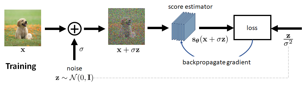
Figure 21: Training of $\mathbf{s}_{\boldsymbol{\theta}}$ for denoising score matching. The network $\mathbf{s}_{\boldsymbol{\theta}}$ is trained to estimate the noise.

The training step can simply described as follows: You give us a training dataset $\{\mathbf{x}^{(\ell)}\}_{\ell=1}^{L}$, we train a network $\boldsymbol{\theta}$ with the goal to

$$\boldsymbol{\theta}^{*}=\mathop{\underset{\boldsymbol{\theta}}{\mbox{argmin}}}\;\;\frac{1}{L}\sum_{\ell=1}^{L}\frac{1}{2}\left\|\mathbf{s}_{\boldsymbol{\theta}}\left(\mathbf{x}^{(\ell)}+\sigma\mathbf{z}^{(\ell)}\right)+\frac{\mathbf{z}^{(\ell)}}{\sigma^{2}}\right\|^{2},\qquad\text{where}\quad\mathbf{z}^{(\ell)}\sim\mathcal{N}(0,\mathbf{I}).$$ (86)

The bigger question here is why Eqn (84) would even make sense in the first place. This needs to be answered through the equivalence between the explicit score matching loss and the denoising score matching loss.

Theorem [Vincent [9]] For up to a constant $C$ which is independent of the variable $\boldsymbol{\theta}$, it holds that $$J_{\text{DSM}}(\boldsymbol{\theta})=J_{\text{ESM}}(\boldsymbol{\theta})+C.$$ (87)

The equivalence between the explicit score matching and the denoising score matching is a major discovery. The proof below is based on the original work of Vincent 2011.

Proof of Eqn (87) We start with the explicit score matching loss function, which is given by $\displaystyle J_{\text{ESM}}(\boldsymbol{\theta})$ $\displaystyle=\mathbb{E}_{q(\mathbf{x})}\left[\frac{1}{2}\left\|\mathbf{s}_{\boldsymbol{\theta}}(\mathbf{x})-\nabla_{\mathbf{x}}\log q(\mathbf{x})\right\|^{2}\right]$ $\displaystyle=\mathbb{E}_{q(\mathbf{x})}\Big{[}\frac{1}{2}\left\|\mathbf{s}_{\boldsymbol{\theta}}(\mathbf{x})\right\|^{2}-\mathbf{s}_{\boldsymbol{\theta}}(\mathbf{x})^{T}\nabla_{\mathbf{x}}\log q(\mathbf{x})+\underset{\overset{\text{def}}{=}C_{1},\text{independent of $\boldsymbol{\theta}$}}{\underbrace{\frac{1}{2}\left\|\nabla_{\mathbf{x}}\log q(\mathbf{x})\right\|^{2}}}\Big{]}.$ Let’s zoom into the second term. We can show that $\displaystyle\mathbb{E}_{q(\mathbf{x})}\left[\mathbf{s}_{\boldsymbol{\theta}}(\mathbf{x})^{T}\nabla_{\mathbf{x}}\log q(\mathbf{x})\right]$ $\displaystyle=\int\left(\mathbf{s}_{\boldsymbol{\theta}}(\mathbf{x})^{T}\nabla_{\mathbf{x}}\log q(\mathbf{x})\right)q(\mathbf{x})d\mathbf{x},$ (expectation) $\displaystyle=\int\left(\mathbf{s}_{\boldsymbol{\theta}}(\mathbf{x})^{T}\frac{\nabla_{\mathbf{x}}q(\mathbf{x})}{\cancel{q(\mathbf{x})}}\right)\cancel{q(\mathbf{x})}d\mathbf{x},$ (gradient) $\displaystyle=\int\mathbf{s}_{\boldsymbol{\theta}}(\mathbf{x})^{T}\nabla_{\mathbf{x}}q(\mathbf{x})d\mathbf{x}.$ Next, we consider conditioning by recalling $q(\mathbf{x})=\int q(\mathbf{x}^{\prime})q(\mathbf{x}|\mathbf{x}^{\prime})d\mathbf{x}^{\prime}$. This will give us $\displaystyle\int\mathbf{s}_{\boldsymbol{\theta}}(\mathbf{x})^{T}\nabla_{\mathbf{x}}{\color[rgb]{0,0,1}q(\mathbf{x})}d\mathbf{x}$ $\displaystyle=\int\mathbf{s}_{\boldsymbol{\theta}}(\mathbf{x})^{T}\nabla_{\mathbf{x}}\underset{=q(\mathbf{x})}{\underbrace{\left(\int q(\mathbf{x}^{\prime})q(\mathbf{x}|\mathbf{x}^{\prime})d\mathbf{x}^{\prime}\right)}}d\mathbf{x}$ (conditional) $\displaystyle=\int\mathbf{s}_{\boldsymbol{\theta}}(\mathbf{x})^{T}\left(\int q(\mathbf{x}^{\prime}){\color[rgb]{0,0,1}\nabla_{\mathbf{x}}}q(\mathbf{x}|\mathbf{x}^{\prime})d\mathbf{x}^{\prime}\right)d\mathbf{x}$ (move gradient) $\displaystyle=\int\mathbf{s}_{\boldsymbol{\theta}}(\mathbf{x})^{T}\left(\int q(\mathbf{x}^{\prime})\nabla_{\mathbf{x}}q(\mathbf{x}|\mathbf{x}^{\prime})\times{\color[rgb]{0,0,1}\frac{q(\mathbf{x}|\mathbf{x}^{\prime})}{q(\mathbf{x}|\mathbf{x}^{\prime})}}d\mathbf{x}^{\prime}\right)d\mathbf{x}$ (multiple and divide) $\displaystyle=\int\mathbf{s}_{\boldsymbol{\theta}}(\mathbf{x})^{T}\int q(\mathbf{x}^{\prime})\underset{=\nabla_{\mathbf{x}}\log q(\mathbf{x}|\mathbf{x}^{\prime})}{\underbrace{\left(\frac{\nabla_{\mathbf{x}}q(\mathbf{x}|\mathbf{x}^{\prime})}{q(\mathbf{x}|\mathbf{x}^{\prime})}\right)}}q(\mathbf{x}|\mathbf{x}^{\prime})d\mathbf{x}^{\prime}d\mathbf{x}$ (rearrange terms) $\displaystyle=\int\mathbf{s}_{\boldsymbol{\theta}}(\mathbf{x})^{T}\left(\int q(\mathbf{x}^{\prime})\Big{(}\nabla_{\mathbf{x}}\log q(\mathbf{x}|\mathbf{x}^{\prime})\Big{)}q(\mathbf{x}|\mathbf{x}^{\prime})d\mathbf{x}^{\prime}\right)d\mathbf{x}$ $\displaystyle=\int\int\underset{=q(\mathbf{x},\mathbf{x}^{\prime})}{\underbrace{q(\mathbf{x}|\mathbf{x}^{\prime})q(\mathbf{x}^{\prime})}}\Big{(}\mathbf{s}_{\boldsymbol{\theta}}(\mathbf{x})^{T}\nabla_{\mathbf{x}}\log q(\mathbf{x}|\mathbf{x}^{\prime})\Big{)}d\mathbf{x}^{\prime}d\mathbf{x}$ (move integration) $\displaystyle=\mathbb{E}_{q(\mathbf{x},\mathbf{x}^{\prime})}\left[\mathbf{s}_{\boldsymbol{\theta}}(\mathbf{x})^{T}\nabla_{\mathbf{x}}\log q(\mathbf{x}|\mathbf{x}^{\prime})\right].$ So, if we substitute this result back to the definition of ESM, we can show that $\displaystyle J_{\text{ESM}}(\boldsymbol{\theta})=\mathbb{E}_{q(\mathbf{x})}\Big{[}\frac{1}{2}\left\|\mathbf{s}_{\boldsymbol{\theta}}(\mathbf{x})\right\|^{2}\Big{]}-\mathbb{E}_{q(\mathbf{x},\mathbf{x}^{\prime})}\left[\mathbf{s}_{\boldsymbol{\theta}}(\mathbf{x})^{T}\nabla_{\mathbf{x}}\log q(\mathbf{x}|\mathbf{x}^{\prime})\right]+C_{1}.$ Comparing this with the definition of DSM, we can observe that $\displaystyle J_{\text{DSM}}(\boldsymbol{\theta})$ $\displaystyle\overset{\text{def}}{=}\mathbb{E}_{q(\mathbf{x},\mathbf{x}^{\prime})}\left[\frac{1}{2}\left\|\mathbf{s}_{\boldsymbol{\theta}}(\mathbf{x})-\nabla_{\mathbf{x}}q(\mathbf{x}|\mathbf{x}^{\prime})\right\|^{2}\right]$ $\displaystyle=\mathbb{E}_{q(\mathbf{x},\mathbf{x}^{\prime})}\Big{[}\frac{1}{2}\left\|\mathbf{s}_{\boldsymbol{\theta}}(\mathbf{x})\right\|^{2}-\mathbf{s}_{\boldsymbol{\theta}}(\mathbf{x})^{T}\nabla_{\mathbf{x}}\log q(\mathbf{x}|\mathbf{x}^{\prime})+\underset{\overset{\text{def}}{=}C_{2},\text{independent of $\boldsymbol{\theta}$}}{\underbrace{\frac{1}{2}\left\|\nabla_{\mathbf{x}}\log q(\mathbf{x}|\mathbf{x}^{\prime})\right\|^{2}}}\Big{]}$ $\displaystyle=\mathbb{E}_{q(\mathbf{x})}\Big{[}\frac{1}{2}\left\|\mathbf{s}_{\boldsymbol{\theta}}(\mathbf{x})\right\|^{2}\Big{]}-\mathbb{E}_{q(\mathbf{x},\mathbf{x}^{\prime})}\left[\mathbf{s}_{\boldsymbol{\theta}}(\mathbf{x})^{T}\nabla_{\mathbf{x}}\log q(\mathbf{x}|\mathbf{x}^{\prime})\right]+C_{2}.$ Therefore, we conclude that $$J_{\text{DSM}}(\boldsymbol{\theta})=J_{\text{ESM}}(\boldsymbol{\theta})-C_{1}+C_{2}.$$

For inference, we assume that we have already trained the score estimator $\mathbf{s}_{\boldsymbol{\theta}}$. To generate an image, we perform the following procedure for $t=1,\ldots,T$:

$$\mathbf{x}_{t+1}=\mathbf{x}_{t}+\tau\mathbf{s}_{\boldsymbol{\theta}}(\mathbf{x}_{t})+\sqrt{2\tau}\mathbf{z}_{t},\qquad\text{where}\quad\mathbf{z}_{t}\sim\mathcal{N}(0,\mathbf{I}).$$ (88)

Congratulations! We are done. This is all about Score-based Generative Models.

Additional readings about score-matching should start with Vincent’s technical report [9]. A very popular paper in the recent literature is Song and Ermon [15], their follow up work [16], and [8]. In practice, training a score function requires a noise schedule by considering a sequence of noise levels. We will briefly discuss this when we explain the variance exploding SDE in the next section.

4 Stochastic Differential Equation (SDE)

Thus far we have derived the diffusion iterations via the DDPM and the SMLD perspective. In this section, we will introduce a third perspective through the lens of differential equation. It may not be obvious why our iterative schemes suddenly become the complicated differential equations. So, before we derive any equation, we should briefly discuss how differential equations can be relevant to us.

4.1 Motivating Examples

Example 1. Simple First-Order ODE. Imagine that we are given a discrete-time algorithm with the iterations defined by the recursion: $$\mathbf{x}_{i}=\left(1-\frac{\beta\Delta t}{2}\right)\mathbf{x}_{i-1},\qquad\text{for}\;\;i=1,2,\ldots,N,$$ (89) for some hyperparameter $\beta$ and a step-size parameter $\Delta t$. This recursion has nothing complicated: You give us $\mathbf{x}_{i-1}$, we update and return you $\mathbf{x}_{i}$. If we assume a discretization scheme of a continuous time function $\mathbf{x}(t)$ by letting $\mathbf{x}_{i}=\mathbf{x}(\tfrac{i}{N})$, $\Delta t=\tfrac{1}{N}$, and $t\in\{0,\tfrac{1}{N},\ldots,\tfrac{N-1}{N}\}$, then we can rewrite the recursion as $\displaystyle\mathbf{x}(t+\Delta t)=\left(1-\frac{\beta\Delta t}{2}\right)\mathbf{x}(t).$ Rearranging the terms will give us $\displaystyle\frac{\mathbf{x}(t+\Delta t)-\mathbf{x}(t)}{\Delta t}=-\frac{\beta}{2}\mathbf{x}(t),$ where at the limit when $\Delta t\rightarrow 0$, we can write the discrete equation as an ordinary differential equation (ODE) $$\frac{d\mathbf{x}(t)}{dt}=-\frac{\beta}{2}\mathbf{x}(t).$$ (90) Not only that, we can solve for an analytic solution for the ODE where the solution is given by $$\mathbf{x}(t)=e^{-\frac{\beta}{2}t}.$$ (91) If you don’t believe us, just substitute Eqn (91) into Eqn (90) and you can show that the equality holds. The power of the ODE is that it offers us an analytic solution. Instead of resorting to the iterative scheme (which will take hundreds to thousands of iterations), the analytic solution tells us exactly the behavior of the solution at any time $t$. To illustrate this fact, we show in the figure below the trajectory of the solution $\mathbf{x}_{1},\mathbf{x}_{2},\ldots,\mathbf{x}_{i},\ldots,\mathbf{x}_{N}$ defined by the algorithm. Here, we choose $\Delta t=0.1$. In the same plot, we directly plot the continuous-time solution $\mathbf{x}(t)=\exp\{-\beta t/2\}$ for arbitrary $t$. As you can see, the analytic solution is exactly the same as the trajectory predicted by the iterative scheme.

What we observe in this motivating example are a two interesting facts:

• The discrete-time iterative scheme can be written as a continuous-time ordinary differential equation. It turns out that for any finite-difference equations, we can turn the recursion into an ODE.

• For simple ODEs, we can write down the analytic solution in closed form. More complicated ODE would be hard to write an analytic solution. But we can still use ODE tools to analyze the behavior of the solution. We can also derive the limiting solution $t\rightarrow 0$.

Example 2: Gradient Descent. Recall that a gradient descent algorithm for a (well-behaved) convex function $f$ is the following recursion. For $i=1,2,\ldots,N$, do $$\mathbf{x}_{i}=\mathbf{x}_{i-1}-\beta_{i-1}\nabla f(\mathbf{x}_{i-1}),$$ (92) for step-size parameter $\beta_{i}$. Using the same discretization as we did in the previous example, we can show that (by letting $\beta_{i-1}=\beta(t)\Delta t$): $\displaystyle\mathbf{x}_{i}=\mathbf{x}_{i-1}-\beta_{i-1}\nabla f(\mathbf{x}_{i-1})$ $\displaystyle\qquad\Longrightarrow\qquad\mathbf{x}(t+\Delta t)=\mathbf{x}(t)-\beta(t)\Delta t\nabla f(\mathbf{x}(t))$ $\displaystyle\qquad\Longrightarrow\qquad\frac{\mathbf{x}(t+\Delta t)-\mathbf{x}(t)}{\Delta t}=-\beta(t)\nabla f(\mathbf{x}(t))$ $\displaystyle\qquad\Longrightarrow\qquad\frac{d\mathbf{x}(t)}{dt}=-\beta(t)\nabla f(\mathbf{x}(t)).$ (93) The ordinary differential equation shown on the right has a solution trajectory $\mathbf{x}(t)$. This $\mathbf{x}(t)$ is known as the gradient flow of the function $f$. For simplicity, we can make $\beta(t)=\beta$ for all $t$. Then there are two simple facts about this ODE. First, we can show that $\displaystyle\frac{d}{dt}f(\mathbf{x}(t))$ $\displaystyle=\nabla f(\mathbf{x}(t))^{T}\frac{d\mathbf{x}(t)}{dt}$ $\displaystyle(\text{chain rule})$ $\displaystyle=\nabla f(\mathbf{x}(t))^{T}\left[-\beta\nabla f(\mathbf{x}(t))\right]$ $\displaystyle(\text{Eqn \eqref{eq: GD ODE main}})$ $\displaystyle=-\beta\nabla f(\mathbf{x}(t))^{T}\nabla f(\mathbf{x}(t))$ $\displaystyle=-\beta\|\nabla f(\mathbf{x}(t))\|^{2}\leq 0$ $\displaystyle(\text{norm-squares}).$ Therefore, as we move from $\mathbf{x}_{i-1}$ to $\mathbf{x}_{i}$, the objective value $f(\mathbf{x}(t))$ has to go down. This is consistent with our expectation because a gradient descent algorithm should bring the cost down as the iteration goes on. Second, at the limit when $t\rightarrow\infty$, we know that $\frac{d\mathbf{x}(t)}{dt}\rightarrow 0$. Hence, $\frac{d\mathbf{x}(t)}{dt}=-\nabla f(\mathbf{x}(t))$ will imply that $$\nabla f(\mathbf{x}(t))\rightarrow 0,\qquad\text{as }t\rightarrow\infty.$$ (94) Therefore, the solution trajectory $\mathbf{x}(t)$ will approach the minimizer for the function $f$.

Forward and Backward Updates.

Let’s use the gradient descent example to illustrate one more aspect of the ODE. Going back to Eqn (92), we recognize that the recursion can be written equivalently as (assuming $\beta(t)=\beta)$:

$$\underset{\Delta\mathbf{x}}{\underbrace{\mathbf{x}_{i}-\mathbf{x}_{i-1}}}=-\underset{\beta\Delta t}{\underbrace{\beta_{i-1}}}\nabla f(\mathbf{x}_{i-1})\;\;\Rightarrow\;\;d\mathbf{x}=-\beta\nabla f(\mathbf{x})dt,$$ (95)

where the continuous equation holds when we set $\Delta t\rightarrow 0$ and $\Delta\mathbf{x}\rightarrow 0$. The interesting point about this equality is that it gives us a summary of the update $\Delta\mathbf{x}$ by writing it in terms of $dt$. It says that if we move the along the time axis by $dt$, then the solution $\mathbf{x}$ will be updated by $d\mathbf{x}$.

Eqn (95) defines the relationship between changes. If we consider a sequence of iterates $i=1,2,\ldots,N$, and if we are told that the progression of the iterates follows Eqn (95), then we can write

$$\text{(forward)}\hskip 56.9055pt\mathbf{x}_{i}=\mathbf{x}_{i-1}+\Delta\mathbf{x}_{i-1} \approx\mathbf{x}_{i-1}+d\mathbf{x}$$

$$=\mathbf{x}_{i-1}-\nabla f(\mathbf{x}_{i-1})\beta dt$$

$$\approx\mathbf{x}_{i-1}-\beta_{i-1}\nabla f(\mathbf{x}_{i-1}).$$

We call this as the forward equation because we update $\mathbf{x}$ by $\mathbf{x}+\Delta\mathbf{x}$ assuming that $t\leftarrow t+\Delta t$.

Now, consider a sequence of iterates $i=N,N-1,\ldots,2,1$. If we are told that the progression of the iterates follows Eqn (95), then the time-reversal iterates will be

$$\text{(reverse)}\hskip 56.9055pt\mathbf{x}_{i-1}=\mathbf{x}_{i}-\Delta\mathbf{x}_{i} \approx\mathbf{x}_{i}+d\mathbf{x}$$

$$=\mathbf{x}_{i}+\beta\nabla f(\mathbf{x}_{i})dt$$

$$\approx\mathbf{x}_{i}+\beta_{i}\nabla f(\mathbf{x}_{i}).$$

Note the change in sign when reversing the progression direction. We call this the reverse equation.

4.2 Forward and Backward Iterations in SDE

The concept of differential equation for diffusion is not too far from the above gradient descent algorithm. If we introduce a noise term $\mathbf{z}_{t}\sim\mathcal{N}(0,\mathbf{I})$ to the gradient descent algorithm, then the ODE will become a stochastic differential equation (SDE). To see this, we just follow the same discretization scheme by defining $\mathbf{x}(t)$ as a continuous function for $0\leq t\leq 1$. Suppose that there are $N$ steps in the interval so that the interval $[0,1]$ can be divided into a sequence $\{\tfrac{i}{N}\,|\,i=0,\ldots,N-1\}$. The discretization will give us $\mathbf{x}_{i}=\mathbf{x}(\tfrac{i}{N})$, and $\mathbf{x}_{i-1}=\mathbf{x}(\tfrac{i-1}{N})$. The interval step is $\Delta t=\tfrac{1}{N}$, and the set of all $t$’s is $t\in\{0,\tfrac{1}{N},\ldots,\tfrac{N-1}{N}\}$. Using these definitions, we can write

$$\mathbf{x}_{i} =\mathbf{x}_{i-1}-\tau\nabla f(\mathbf{x}_{i-1})+\mathbf{z}_{i-1}$$

$$\qquad\Longrightarrow\qquad \mathbf{x}(t+\Delta t) =\mathbf{x}(t)-\tau\nabla f(\mathbf{x}(t))+\mathbf{z}(t).$$

Now, let’s define a random process $\mathbf{w}(t)$ such that $\mathbf{z}(t)=\mathbf{w}(t+\Delta t)-\mathbf{w}(t)\approx\frac{d\mathbf{w}(t)}{dt}\Delta t$ for a very small $\Delta t$. In computation, we can generate such a $\mathbf{w}(t)$ by integrating $\mathbf{z}(t)$ (which is a Wiener process). With $\mathbf{w}(t)$ defined, we can write

$$\mathbf{x}(t+\Delta t) =\mathbf{x}(t)-\tau\nabla f(\mathbf{x}(t))+\mathbf{z}(t)$$

$$\qquad\Longrightarrow\qquad \mathbf{x}(t+\Delta t)-\mathbf{x}(t) =-\tau\nabla f(\mathbf{x}(t))+\mathbf{w}(t+\Delta t)-\mathbf{w}(t)$$

$$\qquad\Longrightarrow\qquad d\mathbf{x} =-\tau\nabla f(\mathbf{x})dt+d\mathbf{w}.$$

The equation above reveals a generic form of the SDE. We summarize it as follows. Forward Diffusion. $$d\mathbf{x}=\underset{\text{drift}}{\underbrace{\mathbf{f}(\mathbf{x},t)}}\;dt+\underset{\text{diffusion}}{\underbrace{g(t)}}\;d\mathbf{w}.$$ (96)

The two terms $\mathbf{f}(\mathbf{x},t)$ and $g(t)$ carry physical meaning. The draft coefficient is a vector-valued function $\mathbf{f}(\mathbf{x},t)$ defining how molecules in a closed system would move in the absence of random effects. For the gradient descent algorithm, the drift is defined by the negative gradient of the objective function. That is, we want the solution trajectory to follow the gradient of the objective.

The diffusion coefficient $g(t)$ is a scalar function describing how the molecules would randomly walk from one position to another. The function $g(t)$ determines how strong the random movement is.

Example. Consider the equation $$d\mathbf{x}=ad\mathbf{w},$$ where $a=0.05$. The iterative scheme can be written as $\displaystyle\mathbf{x}_{i}-\mathbf{x}_{i-1}=a\underset{\overset{\text{def}}{=}\mathbf{z}_{i-1}\sim\mathcal{N}(0,\mathbf{I})}{\underbrace{(\mathbf{w}_{i}-\mathbf{w}_{i-1})}}\quad\Rightarrow\quad\mathbf{x}_{i}=\mathbf{x}_{i-1}+a\mathbf{z}_{i}.$ We can plot the function $\mathbf{x}_{i}$ as below. The initial point $\mathbf{x}_{0}=0$ is marked as in red to indicate that the process is moving forward in time.

Remark. As you can see, the differential $d\mathbf{w}=\mathbf{w}_{i}-\mathbf{w}_{i-1}$ is defined as the Wiener process which is a white Gaussian vector. The individual $\mathbf{w}_{i}$ is not a Gaussian, but the difference $\mathbf{w}_{i}-\mathbf{w}_{i-1}$ is a Gaussian.

Example. Consider the equation $$d\mathbf{x}=-\frac{\alpha}{2}\mathbf{x}dt+\beta d\mathbf{w},$$ where $\alpha=1$ and $\beta=0.1$. This equation can be written as $\displaystyle\mathbf{x}_{i}-\mathbf{x}_{i-1}=-\frac{\alpha}{2}\mathbf{x}_{i-1}+\beta\underset{\overset{\text{def}}{=}\mathbf{z}_{i-1}\sim\mathcal{N}(0,\mathbf{I})}{\underbrace{(\mathbf{w}_{i}-\mathbf{w}_{i-1})}}\quad\Rightarrow\quad\mathbf{x}_{i}=\left(1-\frac{\alpha}{2}\right)\mathbf{x}_{i-1}+\beta\mathbf{z}_{i-1}.$ We can plot the function $\mathbf{x}_{i}$ as below.

The reverse direction of the diffusion equation is to move backward in time. The reverse-time SDE, according to Anderson [17], is given as follows. Reverse SDE. $$d\mathbf{x}=[\underset{\text{drift}}{\underbrace{\mathbf{f}(\mathbf{x},t)}}-g(t)^{2}\underset{\text{score function}}{\underbrace{\nabla_{\mathbf{x}}\log p_{t}(\mathbf{x})}}]\;dt\;\;\;\;+\underset{\text{reverse-time diffusion}}{\underbrace{g(t)d\overline{\mathbf{w}}}},$$ (97) where $p_{t}(\mathbf{x})$ is the probability distribution of $\mathbf{x}$ at time $t$, and $\overline{\mathbf{w}}$ is the Wiener process when time flows backward.

Example. Consider the reverse diffusion equation $$d\mathbf{x}=ad\overline{\mathbf{w}}.$$ (98) We can write the discrete-time recursion as follows. For $i=N,N-1,\ldots,1$, do $\displaystyle\mathbf{x}_{i-1}=\mathbf{x}_{i}+a\underset{=\mathbf{z}_{i}}{\underbrace{(\mathbf{w}_{i-1}-\mathbf{w}_{i})}}=\mathbf{x}_{i}+a\mathbf{z}_{i},\quad\mathbf{z}_{i}\sim\mathcal{N}(0,\mathbf{I}).$ In the figure below we show the trajectory of this reverse-time process. Note that the initial point marked in red is at $\mathbf{x}_{N}$. The process is tracked backward to $\mathbf{x}_{0}$.

4.3 Stochastic Differential Equation for DDPM

In order to draw the connection between DDPM and SDE, we consider the discrete-time DDPM iteration. For $i=1,2,\ldots,N$:

$$\mathbf{x}_{i}=\sqrt{1-\beta_{i}}\mathbf{x}_{i-1}+\sqrt{\beta_{i}}\mathbf{z}_{i-1},\qquad\mathbf{z}_{i-1}\sim\mathcal{N}(0,\mathbf{I}).$$ (99)

We can show that this equation can be derived from the forward SDE equation below. The forward sampling equation of DDPM can be written as an SDE via $$d\mathbf{x}=\underset{=\mathbf{f}(\mathbf{x},t)}{\underbrace{-\frac{\beta(t)}{2}\;\mathbf{x}}}\;dt+\underset{=g(t)}{\underbrace{\sqrt{\beta(t)}}}d\mathbf{w}.$$ (100)

To see why this is the case, we define a step size $\Delta t=\tfrac{1}{N}$, and consider an auxiliary noise level $\{\overline{\beta}_{i}\}_{i=1}^{N}$ where $\beta_{i}=\tfrac{\overline{\beta}_{i}}{N}$. Then

$$\beta_{i}=\underset{\overline{\beta}_{i}}{\underbrace{\beta\left(\tfrac{i}{N}\right)}}\cdot\frac{1}{N}=\beta(t+\Delta t)\Delta t,$$

where we assume that in the $N\rightarrow\infty$, $\overline{\beta}_{i}=\rightarrow\beta(t)$ which is a continuous time function for $0\leq t\leq 1$. Similarly, we define

$$\mathbf{x}_{i}=\mathbf{x}\left(\tfrac{i}{N}\right)=\mathbf{x}(t+\Delta t),\quad\mathbf{z}_{i}=\mathbf{z}\left(\tfrac{i}{N}\right)=\mathbf{z}(t+\Delta t).$$

Hence, we have

$$\mathbf{x}_{i} =\sqrt{1-\beta_{i}}\mathbf{x}_{i-1}+\sqrt{\beta_{i}}\mathbf{z}_{i-1}$$

$$\Rightarrow\qquad \mathbf{x}_{i} =\sqrt{1-\tfrac{\overline{\beta}_{i}}{N}}\mathbf{x}_{i-1}+\sqrt{\tfrac{\overline{\beta}_{i}}{N}}\mathbf{z}_{i-1}$$

$$\Rightarrow\qquad \mathbf{x}(t+\Delta t) =\sqrt{1-\beta(t+\Delta t)\cdot\Delta t}\;\mathbf{x}(t)+\sqrt{\beta(t+\Delta t)\cdot\Delta t}\;\mathbf{z}(t)$$

$$\Rightarrow\qquad \mathbf{x}(t+\Delta t) \approx\left(1-\frac{1}{2}\beta(t+\Delta t)\cdot\Delta t\right)\;\mathbf{x}(t)+\sqrt{\beta(t+\Delta t)\cdot\Delta t}\;\mathbf{z}(t)$$

$$\Rightarrow\qquad \mathbf{x}(t+\Delta t) \approx\mathbf{x}(t)-\frac{1}{2}\beta(t)\Delta t\;\mathbf{x}(t)+\sqrt{\beta(t)\cdot\Delta t}\;\mathbf{z}(t).$$

Thus, as $\Delta t\rightarrow 0$, we have

$$d\mathbf{x}=-\frac{1}{2}\beta(t)\mathbf{x}dt+\sqrt{\beta(t)}\;d\mathbf{w}.$$ (101)

Therefore, we showed that the DDPM forward update iteration can be equivalently written as an SDE.

Being able to write the DDPM forward update iteration as an SDE means that the DDPM estimates can be determined by solving the SDE. In other words, for an appropriately defined SDE solver, we can throw the SDE into the solver. The solution returned by an appropriately chosen solver will be the DDPM estimate. Of course, we are not required to use the SDE solver because the DDPM iteration itself is solving the SDE. It may not be the best SDE solver because the DDPM iteration is only a first order method. Nevertheless, if we are not interested in using the SDE solver, we can still use the DDPM iteration to obtain a solution. Here is an example.

Example. Consider the DDPM forward equation with $\beta_{i}=0.05$ for all $i=0,\ldots,N-1$. We initialize the sample $\mathbf{x}_{0}$ by drawing it from a Gaussian mixture such that $$\mathbf{x}_{0}\sim\sum_{k=1}^{K}\pi_{k}\mathcal{N}(\mathbf{x}_{0}|\boldsymbol{\mu}_{k},\sigma_{k}^{2}\mathbf{I}),$$ where $\pi_{1}=\pi_{2}=0.5$, $\sigma_{1}=\sigma_{2}=1$, $\boldsymbol{\mu}_{1}=3$ and $\boldsymbol{\mu}_{2}=-3$. Then, using the equation $$\mathbf{x}_{i}=\sqrt{1-\beta_{i}}\mathbf{x}_{i-1}+\sqrt{\beta_{i}}\mathbf{z}_{i-1},\qquad\mathbf{z}_{i-1}\sim\mathcal{N}(0,\mathbf{I}),$$ we can plot the trajectory and the distribution as follows.

The reverse diffusion equation follows from Eqn (97) by substituting the appropriate quantities: $\mathbf{f}(\mathbf{x},t)=-\frac{\beta(t)}{2}$ and $g(t)=\sqrt{\beta(t)}$. This will give us

$$d\mathbf{x} =[\mathbf{f}(\mathbf{x},t)-g(t)^{2}\nabla_{\mathbf{x}}\log p_{t}(\mathbf{x})]dt+g(t)d\overline{\mathbf{w}}$$

$$=\left[-\frac{\beta(t)}{2}\;\mathbf{x}-\beta(t)\nabla_{\mathbf{x}}\log p_{t}(\mathbf{x})\right]dt+\sqrt{\beta(t)}d\overline{\mathbf{w}},$$

which will give us the following equation: The reverse sampling equation of DDPM can be written as an SDE via $$d\mathbf{x}=-\beta(t)\left[\frac{\mathbf{x}}{2}+\nabla_{\mathbf{x}}\log p_{t}(\mathbf{x})\right]dt+\sqrt{\beta(t)}d\overline{\mathbf{w}}.$$ (102)

The iterative update scheme can be written by considering $d\mathbf{x}=\mathbf{x}(t)-\mathbf{x}(t-\Delta t)$, and $d\overline{\mathbf{w}}=\mathbf{w}(t-\Delta t)-\mathbf{w}(t)=-\mathbf{z}(t)$. Then, letting $dt=\Delta t$, we can show that

$$\mathbf{x}(t)-\mathbf{x}(t-\Delta t) =-\beta(t)\Delta t\left[\frac{\mathbf{x}(t)}{2}+\nabla_{\mathbf{x}}\log p_{t}(\mathbf{x}(t))\right]-\sqrt{\beta(t)\Delta t}\mathbf{z}(t)$$

$$\Rightarrow\quad \mathbf{x}(t-\Delta t) =\mathbf{x}(t)+\beta(t)\Delta t\left[\frac{\mathbf{x}(t)}{2}+\nabla_{\mathbf{x}}\log p_{t}(\mathbf{x}(t))\right]+\sqrt{\beta(t)\Delta t}\mathbf{z}(t).$$

By grouping the terms, and assuming that $\beta(t)\Delta t\ll 1$, we recognize that

$$\mathbf{x}(t-\Delta t) =\mathbf{x}(t)\left[1+\frac{\beta(t)\Delta t}{2}\right]+\beta(t)\Delta t\nabla_{\mathbf{x}}\log p_{t}(\mathbf{x}(t))+\sqrt{\beta(t)\Delta t}\mathbf{z}(t)$$

$$\approx\mathbf{x}(t)\left[1+\frac{\beta(t)\Delta t}{2}\right]+\beta(t)\Delta t\nabla_{\mathbf{x}}\log p_{t}(\mathbf{x}(t))+{\color[rgb]{0,0,1}\tfrac{(\beta(t)\Delta t)^{2}}{2}\nabla_{\mathbf{x}}\log p_{t}(\mathbf{x}(t))}+\sqrt{\beta(t)\Delta t}\mathbf{z}(t)$$

$$=\left[1+\frac{\beta(t)\Delta t}{2}\right]\Big{(}\mathbf{x}(t)+\beta(t)\Delta t\nabla_{\mathbf{x}}\log p_{t}(\mathbf{x}(t))\Big{)}+\sqrt{\beta(t)\Delta t}\mathbf{z}(t).$$

Then, following the discretization scheme by letting $t\in\{0,\ldots,\frac{N-1}{N}\}$, $\Delta t=1/N$, $\mathbf{x}(t-\Delta t)=\mathbf{x}_{i-1}$, $\mathbf{x}(t)=\mathbf{x}_{i}$, and $\beta(t)\Delta t=\beta_{i}$, we can show that

$$\mathbf{x}_{i-1} =(1+\tfrac{\beta_{i}}{2})\Big{[}\mathbf{x}_{i}+\tfrac{\beta_{i}}{2}\nabla_{\mathbf{x}}\log p_{i}(\mathbf{x}_{i})\Big{]}+\sqrt{\beta_{i}}\mathbf{z}_{i}$$

$$\approx\tfrac{1}{\sqrt{1-\beta_{i}}}\Big{[}\mathbf{x}_{i}+\tfrac{\beta_{i}}{2}\nabla_{\mathbf{x}}\log p_{i}(\mathbf{x}_{i})\Big{]}+\sqrt{\beta_{i}}\mathbf{z}_{i},$$ (103)

where $p_{i}(\mathbf{x})$ is the probability density function of $\mathbf{x}$ at time $i$. For practical implementation, we can replace $\nabla_{\mathbf{x}}\log p_{i}(\mathbf{x}_{i})$ by the estimated score function $\mathbf{s}_{\boldsymbol{\theta}}(\mathbf{x}_{i})$.

So, we have recovered the DDPM iteration that is consistent with the one defined by Song and Ermon in [8]. This is an interesting result, because it allows us to connect DDPM’s iteration using the score function. Song and Ermon [8] called the SDE an variance preserving (VP) SDE.

Example. Following from the previous example, we perform the reverse diffusion equation using $$\mathbf{x}_{i-1}=\tfrac{1}{\sqrt{1-\beta_{i}}}\Big{[}\mathbf{x}_{i}+\tfrac{\beta_{i}}{2}\nabla_{\mathbf{x}}\log p_{i}(\mathbf{x}_{i})\Big{]}+\sqrt{\beta_{i}}\mathbf{z}_{i},$$ where $\mathbf{z}_{i}\sim\mathcal{N}(0,\mathbf{I})$. The trajectory of the iterates is shown below.

4.4 Stochastic Differential Equation for SMLD

The score-matching Langevin Dynamics model can also be described by an SDE. To start with, we notice that in the SMLD setting, there isn’t really a “forward diffusion step”. However, we can roughly argue that if we divide the noise scale in the SMLD training into $N$ levels, then the recursion should follow a Markov chain

$$\mathbf{x}_{i}=\mathbf{x}_{i-1}+\sqrt{\sigma_{i}^{2}-\sigma_{i-1}^{2}}\mathbf{z}_{i-1},\qquad i=1,2,\ldots,N.$$ (104)

This is not too hard to see. If we assume that the variance of $\mathbf{x}_{i-1}$ is $\sigma_{i-1}^{2}$, then we can show that

$$\mathrm{Var}[\mathbf{x}_{i}] =\mathrm{Var}[\mathbf{x}_{i-1}]+(\sigma_{i}^{2}-\sigma_{i-1}^{2})$$

$$=\sigma_{i-1}^{2}+(\sigma_{i}^{2}-\sigma_{i-1}^{2})=\sigma_{i}^{2}.$$

Therefore, given a sequence of noise levels, Eqn (104) will indeed generate estimates $\mathbf{x}_{i}$ such that the noise statistics will satisfy the desired property.

If we agree Eqn (104), it is easy to derive the SDE associated with Eqn (104). Assuming that in the limit $\{\sigma_{i}\}_{i=1}^{N}$ becomes the continuous time $\sigma(t)$ for $0\leq t\leq 1$, and $\{\mathbf{x}_{i}\}_{i=1}^{N}$ becomes $\mathbf{x}(t)$ where $\mathbf{x}_{i}=\mathbf{x}(\tfrac{i}{N})$ if we let $t\in\{0,\tfrac{1}{N},\ldots,\tfrac{N-1}{N}\}$. Then we have

$$\mathbf{x}(t+\Delta t) =\mathbf{x}(t)+\sqrt{\sigma(t+\Delta t)^{2}-\sigma(t)^{2}}\mathbf{z}(t)$$

$$\approx\mathbf{x}(t)+\sqrt{\frac{d[\sigma(t)^{2}]}{dt}\Delta t}\;\mathbf{z}(t).$$

At the limit when $\Delta t\rightarrow 0$, the equation converges to

$$d\mathbf{x}=\sqrt{\frac{d[\sigma(t)^{2}]}{dt}}\;d\mathbf{w}.$$

We summarize our result as follows. The forward sampling equation of SMLD can be written as an SDE via $$d\mathbf{x}=\sqrt{\frac{d[\sigma(t)^{2}]}{dt}}\;d\mathbf{w}.$$ (105) Mapping this to Eqn (96), we recognize that

$$\mathbf{f}(\mathbf{x},t)=0,\qquad\text{and}\qquad g(t)=\sqrt{\frac{d[\sigma(t)^{2}]}{dt}}.$$

As a result, if we write the reverse equation Eqn (97), we should have

$$d\mathbf{x} =[\mathbf{f}(\mathbf{x},t)-g(t)^{2}\nabla_{\mathbf{x}}\log p_{t}(\mathbf{x})]\;dt\;\;+\;\;g(t)d\overline{\mathbf{w}}$$

$$=-\left(\frac{d[\sigma(t)^{2}]}{dt}\nabla_{\mathbf{x}}\log p_{t}(\mathbf{x}(t))\right)dt+\sqrt{\frac{d[\sigma(t)^{2}]}{dt}}\;d\overline{\mathbf{w}}.$$

This will give us the following reverse equation: The reverse sampling equation of SMLD can be written as an SDE via $$d\mathbf{x}=-\left(\frac{d[\sigma(t)^{2}]}{dt}\nabla_{\mathbf{x}}\log p_{t}(\mathbf{x}(t))\right)dt+\sqrt{\frac{d[\sigma(t)^{2}]}{dt}}\;d\overline{\mathbf{w}}.$$ (106) For the discrete-time iterations, we first define $\alpha(t)=\frac{d[\sigma(t)^{2}]}{dt}$. Then, using the same set of discretization setups as the DDPM case, we can show that

$$\mathbf{x}(t+\Delta t)-\mathbf{x}(t) =-\Big{(}\alpha(t)\nabla_{\mathbf{x}}\log p_{t}(\mathbf{x})\Big{)}\Delta t-\sqrt{\alpha(t)\Delta t}\;\mathbf{z}(t)$$

$$\Rightarrow\quad \mathbf{x}(t) =\mathbf{x}(t+\Delta t)+\alpha(t)\Delta t\nabla_{\mathbf{x}}\log p_{t}(\mathbf{x})+\sqrt{\alpha(t)\Delta t}\;\mathbf{z}(t)$$

$$\Rightarrow\quad \mathbf{x}_{i-1} =\mathbf{x}_{i}+\alpha_{i}\nabla_{\mathbf{x}}\log p_{i}(\mathbf{x}_{i})+\sqrt{\alpha_{i}}\;\mathbf{z}_{i}$$ (107)

$$\Rightarrow\quad \mathbf{x}_{i-1} =\mathbf{x}_{i}+(\sigma_{i}^{2}-\sigma_{i-1}^{2})\nabla_{\mathbf{x}}\log p_{i}(\mathbf{x}_{i})+\sqrt{(\sigma_{i}^{2}-\sigma_{i-1}^{2})}\;\mathbf{z}_{i},$$

which is identical to the SMLD reverse update equation. Song and Ermon [8] called the SDE an variance exploding (VE) SDE.

4.5 Solving SDE

In this subsection, we briefly discuss how the differential equations are solved numerically. To make our discussion slightly easier, we shall focus on the ODE. Consider the following ODE

$$\frac{d\mathbf{x}(t)}{dt}=\mathbf{f}(\mathbf{x}(t),t).$$ (108)

If the ODE is a scalar ODE, then the ODE is $\frac{dx(t)}{dt}=f(x(t),t)$.

Euler Method. Euler method is a first order numerical method for solving the ODE. Given $\frac{dx(t)}{dt}=f(x(t),t)$, and $x(t_{0})=x_{0}$, Euler method solves the problem via an iterative scheme for $i=0,1,\ldots,N-1$ such that

$$x_{i+1}=x_{i}+\alpha\cdot f(x_{i},t_{i}),\qquad 0,1,\ldots,N-1,$$

where $\alpha$ is the step size. Let’s consider a simple example.

Example. [18, Example 2.2] Consider the following ODE $$\frac{dx(t)}{dt}=\frac{x(t)+t^{2}-2}{t+1}.$$ If we apply the Euler method with a step size $\alpha$, then the iteration will take the form $\displaystyle x_{i+1}=x_{i}+\alpha\cdot f(x_{i},t_{i})=x_{i}+\alpha\cdot\frac{(x_{i}+t_{i}^{2}-2)}{t_{i}+1}.$

Runge-Kutta (RK) Method. Another popularly used ODE solver is the Runge-Kutta (RK) method. The classical RK-4 algorithm solves the ODE via the iteration

$$x_{i+1}=x_{i}+\frac{\alpha}{6}\cdot\Big{(}k_{1}+2k_{2}+2k_{3}+k_{4}\Big{)},\qquad i=1,2,\ldots,N,$$

where the quantities $k_{1}$, $k_{2}$, $k_{3}$ and $k_{4}$ are defined as

$$k_{1} =f(x_{i},t_{i}),$$

$$k_{2} =f\left(x_{i}+\alpha\tfrac{k_{1}}{2},\;t_{i}+\tfrac{\alpha}{2}\right),$$

$$k_{3} =f\left(x_{i}+\alpha\tfrac{k_{2}}{2},\;t_{i}+\tfrac{\alpha}{2}\right),$$

$$k_{4} =f\left(x_{i}+\alpha k_{3},\;t_{i}+\alpha\right).$$

For more details, you can consult numerical methods textbooks such as [18].

Predictor-Corrector Algorithm. Since different numerical solvers have different behavior in terms of the error of approximation, throwing the ODE (or SDE) into an off-the-shelf numerical solver will result in various degrees of error [19]. However, if we are specifically trying to solve the reverse diffusion equation, it is possible to use techniques other than numerical ODE/SDE solvers to make the appropriate corrections, as illustrated in Figure 22.

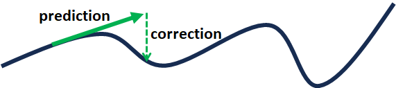
Figure 22: Prediction and correction algorithm.

Let’s use DDPM as an example. In DDPM, the reverse diffusion equation is given by

$$\mathbf{x}_{i-1}=\tfrac{1}{\sqrt{1-\beta_{i}}}\Big{[}\mathbf{x}_{i}+\tfrac{\beta_{i}}{2}\nabla_{\mathbf{x}}\log p_{i}(\mathbf{x}_{i})\Big{]}+\sqrt{\beta_{i}}\mathbf{z}_{i}.$$

We can consider it as an Euler method for the reverse diffusion. However, if we have already trained the score function $\mathbf{s}_{\boldsymbol{\theta}}(\mathbf{x}_{i},i)$, we can run the score-matching equation, i.e.,

$$\mathbf{x}_{i-1}=\mathbf{x}_{i}+\epsilon_{i}\mathbf{s}_{\boldsymbol{\theta}}(\mathbf{x}_{i},i)+\sqrt{2\epsilon_{i}}\mathbf{z}_{i},$$

for $M$ times to make the correction. Algorithm 1 summarizes the idea. (Note that we have replaced the score function by the estimate.)

Algorithm 1 Prediction Correction Algorithm for DDPM.

  $\mathbf{x}_{N}=\mathcal{N}(0,\mathbf{I})$.

  for $i=N-1,\ldots,0$ do

     

$$(\text{Prediction})\qquad\mathbf{x}_{i-1}=\tfrac{1}{\sqrt{1-\beta_{i}}}\Big{[}\mathbf{x}_{i}+\tfrac{\beta_{i}}{2}\mathbf{s}_{\boldsymbol{\theta}}(\mathbf{x}_{i},i)\Big{]}+\sqrt{\beta_{i}}\mathbf{z}_{i}.$$ (109)

     for $m=1,\ldots,M$ do

        

$$(\text{Correction})\qquad\mathbf{x}_{i-1}=\mathbf{x}_{i}+\epsilon_{i}\mathbf{s}_{\boldsymbol{\theta}}(\mathbf{x}_{i},i)+\sqrt{2\epsilon_{i}}\mathbf{z}_{i},$$ (110)

     end for

  end for

For the SMLD algorithm, the two equations are:

$$\mathbf{x}_{i-1} =\mathbf{x}_{i}+(\sigma_{i}^{2}-\sigma_{i-1}^{2})\mathbf{s}_{\boldsymbol{\theta}}(\mathbf{x}_{i},\sigma_{i})+\sqrt{\sigma_{i}^{2}-\sigma_{i-1}^{2}}\mathbf{z} \text{Prediction},$$

$$\mathbf{x}_{i-1} =\mathbf{x}_{i}+\epsilon_{i}\nabla_{\mathbf{x}}\mathbf{s}_{\boldsymbol{\theta}}(\mathbf{x}_{i},\sigma_{i})+\sqrt{\epsilon_{i}}\;\mathbf{z} \text{Correction}.$$

We can pair them up as in the case of DDPM’s prediction-correction algorithm by repeating the correction iteration a few times.

Accelerate the SDE Solver. While generic ODE solvers can be used to solve the ODE, the forward and reverse diffusion equations we encounter are quite special. In fact, they take the form of

$$\frac{d\mathbf{x}(t)}{dt}=\mathbf{a}(t)\mathbf{x}(t)+\mathbf{b}(t),\qquad\mathbf{x}(t_{0})=\mathbf{x}_{0},$$ (111)

for some choice of functions $\mathbf{a}(t)$ and $\mathbf{b}(t)$, with the initial condition $\mathbf{x}(t_{0})=\mathbf{x}_{0}$. This is not a complicated ODE. It is just a first order ODE. In [20], Lu et al. observed that because of the special structure of the ODE (they called the semi-linear structure), it is possible to separately handle $\mathbf{a}(t)\mathbf{x}(t)$ and $\mathbf{b}(t)$. To understand how things work, we use a textbook result shown below. Theorem [Variation of Constants] ([21, Theorem 1.2.3]). Consider the ODE over the range $[s,t]$: $$\frac{dx(t)}{dt}=a(t)x(t)+b(t),\qquad\text{where}\;\;x(t_{0})=x_{0}.$$ (112) The solution is given by $$x(t)=x_{0}e^{A(t)}+e^{A(t)}\int_{t_{0}}^{t}e^{-A(\tau)}b(\tau)d\tau.$$ (113) where $A(t)=\int_{t_{0}}^{t}a(\tau)d\tau$. We can further simplify the second term above by noticing that

$$e^{A(t)-A(\tau)} =e^{\int_{t_{0}}^{t}a(r)dr-\int_{t_{0}}^{\tau}a(r)dr}=e^{\int_{\tau}^{t}a(r)dr}.$$

Of particular interest as presented in [20] was the reverse diffusion equation derived from [8]:

$$\frac{d\mathbf{x}(t)}{dt}=f(t)\mathbf{x}(t)+\frac{g^{2}(t)}{2\sigma(t)}\boldsymbol{\epsilon}_{\boldsymbol{\theta}}(\mathbf{x}(t),t),\qquad\mathbf{x}(t)\sim\mathcal{N}(0,\widetilde{\sigma}^{2}\mathbf{I}),$$

where $f(t)=\frac{d\log\alpha(t)}{dt}$, and $g^{2}(t)=\frac{d\sigma(t)^{2}}{dt}-2\frac{d\log\alpha(t)}{dt}\sigma(t)^{2}$. Using the Variation of Constants Theorem, we can solve the ODE exactly at time $t$ by the formula

$$\mathbf{x}(t)=e^{\int_{s}^{t}f(\tau)d\tau}\mathbf{x}(s)+\int_{s}^{t}\left(e^{\int_{\tau}^{t}f(r)dr}\frac{g^{2}(\tau)}{2\sigma(\tau)}\boldsymbol{\epsilon}_{\boldsymbol{\theta}}(\mathbf{x}(\tau),\tau)\right)d\tau.$$

Then, by defining $\lambda_{t}=\log\alpha(t)/\sigma(t)$, and with additional simplifications outlined in [20], this equation can be simplified to

$$\mathbf{x}(t)=\frac{\alpha(t)}{\alpha(s)}\mathbf{x}(s)-\alpha(t)\int_{s}^{t}\left(\frac{d\lambda_{\tau}}{d\tau}\right)\frac{\sigma(\tau)}{\alpha(\tau)}\boldsymbol{\epsilon}_{\boldsymbol{\theta}}(\mathbf{x}(tau))d\tau.$$

To evaluate this equation, one just needs to run a numerical integrator for the integration shown on the right hand side. Of course, there are other numerical acceleration methods for solving ODEs which we shall skip for brevity.

Congratulations! We are done. This is all about SDE.

Some of you may wonder: Why do we want to map the iterative schemes to differential equations? There are several reasons, some are legitimate whereas some are speculative.

• By unifying multiple diffusion models to the same SDE framework, one can compare the algorithms. In some cases, one can improve the numerical scheme by borrowing ideas from the SDE literature as well as the probabilistic sampling literature. For example, the predictor-corrector scheme in [8] was a hybrid SDE solver coupled with a Markov Chain Monte Carlo.

• Mapping the diffusion iterations to SDE, according to some papers such as [22], offers more design flexibility.

• Outside the context diffusion algorithms, in general stochastic gradient descent algorithms have corresponding SDE such as the Fokker-Planck equations. People have demonstrated how to theoretically analyze the limiting distribution of the estimates, in exact closed-form. This alleviates the difficulty of analyzing the random algorithm by means of analyzing a well-defined limiting distribution.

5 Conclusion

This tutorial covers a few basic concepts underpinning the development of diffusion-based generative models in the recent literature. Given the sheer volume (and quickly expanding) of literature, we find it particularly important to describe the fundamental ideas instead of recycling the Python demos. A few lessons we learned from writing this tutorial are:

• The same diffusion idea can be derived independently from multiple perspectives, namely VAE, DDPM, SMLD, and SDE. There is no particular reason why one is more superior/inferior than the other although some may argue differently.

• The main reason why denoising diffusion works is because of its small increment which was not realized in the age of GAN and VAE.

• Although iterative denoising is the current state-of-the-art, the approach itself does not appear to be the ultimate solution. Humans do not generate images from pure noise. Moreover, because of the small increment nature of diffusion models, speed will continue to be a major hurdle although some efforts in knowledge distillation have been made to improve the situation.

• Some questions regarding generating noise from non-Gaussian might require justification. If the whole reason of introducing Gaussian distribution is to make the derivations easier, why should we switch to another type of noise by making our lives harder?

• Application of diffusion models to inverse problem is readily available. For any existing inverse solvers such as the Plug-and-Play ADMM algorithm, we can replace the denoiser by an explicit diffusion sampler. People have demonstrated improved image restoration results based on this approach.

References

- [1] D. P. Kingma and M. Welling, “An introduction to variational autoencoders,” Foundations and Trends in Machine Learning, vol. 12, no. 4, pp. 307–392, 2019. https://arxiv.org/abs/1906.02691.
- [2] C. Doersch, “Tutorial on variational autoencoders,” 2016. https://arxiv.org/abs/1606.05908.
- [3] D. P. Kingma and M. Welling, “Auto-encoding variational Bayes,” in ICLR, 2014. https://openreview.net/forum?id=33X9fd2-9FyZd.
- [4] J. Ho, A. Jain, and P. Abbeel, “Denoising diffusion probabilistic models,” in NeurIPS, 2020. https://arxiv.org/abs/2006.11239.
- [5] D. P. Kingma, T. Salimans, B. Poole, and J. Ho, “Variational diffusion models,” in NeurIPS, 2021. https://arxiv.org/abs/2107.00630.
- [6] M. Delbracio and P. Milanfar, “Inversion by direct iteration: An alternative to denoising diffusion for image restoration,” Transactions on Machine Learning Research, 2023. https://openreview.net/forum?id=VmyFF5lL3F.
- [7] S. H. Chan, Introduction to Probability for Data Science. Michigan Publishing, 2021. https://probability4datascience.com/.
- [8] Y. Song, J. Sohl-Dickstein, D. P. Kingma, A. Kumar, S. Ermon, and B. Poole, “Score-based generative modeling through stochastic differential equations,” in ICLR, 2021. https://openreview.net/forum?id=PxTIG12RRHS.
- [9] P. Vincent, “A connection between score matching and denoising autoencoders,” Neural Computation, vol. 23, no. 7, pp. 1661–1674, 2011. https://www.iro.umontreal.ca/~vincentp/Publications/smdae_techreport.pdf.
- [10] J. Sohl-Dickstein, E. Weiss, N. Maheswaranathan, and S. Ganguli, “Deep unsupervised learning using nonequilibrium thermodynamics,” in ICML, vol. 37, pp. 2256–2265, 2015. https://arxiv.org/abs/1503.03585.
- [11] C. Luo, “Understanding diffusion models: A unified perspective,” 2022. https://arxiv.org/abs/2208.11970.
- [12] J. Song, C. Meng, and S. Ermon, “Denoising diffusion implicit models,” in ICLR, 2023. https://openreview.net/forum?id=St1giarCHLP.
- [13] R. Rombach, A. Blattmann, D. Lorenz, P. Esser, and B. Ommer, “High-resolution image synthesis with latent diffusion models,” in CVPR, pp. 10684–10695, 2022. https://arxiv.org/abs/2112.10752.
- [14] C. Saharia, W. Chan, S. Saxena, L. Li, J. Whang, E. L. Denton, K. Ghasemipour, R. Gontijo Lopes, B. Karagol Ayan, T. Salimans, J. Ho, D. J. Fleet, and M. Norouzi, “Photorealistic text-to-image diffusion models with deep language understanding,” in NeurIPS, vol. 35, pp. 36479–36494, 2022. https://arxiv.org/abs/2205.11487.
- [15] Y. Song and S. Ermon, “Generative modeling by estimating gradients of the data distribution,” in NeurIPS, 2019. https://arxiv.org/abs/1907.05600.
- [16] Y. Song and S. Ermon, “Improved techniques for training score-based generative models,” in NeurIPS, 2020. https://arxiv.org/abs/2006.09011.
- [17] B. Anderson, “Reverse-time diffusion equation models,” Stochastic Process. Appl., vol. 12, pp. 313–326, May 1982. https://www.sciencedirect.com/science/article/pii/0304414982900515.
- [18] K. Atkinson, W. Han, and D. Stewart, Numerical solution of ordinary differential equations. Wiley, 2009. https://homepage.math.uiowa.edu/~atkinson/papers/NAODE_Book.pdf.
- [19] T. Karras, M. Aittala, T. Aila, and S. Laine, “Elucidating the design space of diffusion-based generative models,” in NeurIPS, 2022. https://arxiv.org/abs/2206.00364.
- [20] C. Lu, Y. Zhou, F. Bao, J. Chen, C. Li, and J. Zhu, “DPM-Solver: A fast ODE solver for diffusion probabilistic model sampling in around 10 steps,” in NeurIPS, 2022. https://arxiv.org/abs/2206.00927.
- [21] G. Nagy, “MTH 235 differential equations,” 2024. https://users.math.msu.edu/users/gnagy/teaching/ade.pdf.
- [22] M. S. Albergo, N. M. Boffi, and E. Vanden-Eijnden, “Stochastic interpolants: A unifying framework for flows and diffusions.” https://arxiv.org/abs/2303.08797.