Goal-Oriented Bayesian Optimal Experimental Design for Nonlinear Models using Markov Chain Monte Carlo
Abstract
Optimal experimental design (OED) provides a systematic approach to quantify and maximize the value of experimental data. Under a Bayesian approach, conventional OED maximizes the expected information gain (EIG) on model parameters. However, we are often interested in not the parameters themselves, but predictive quantities of interest (QoIs) that depend on the parameters in a nonlinear manner. We present a computational framework of predictive goal-oriented OED (GO-OED) suitable for nonlinear observation and prediction models, which seeks the experimental design providing the greatest EIG on the QoIs. In particular, we propose a nested Monte Carlo estimator for the QoI EIG, featuring Markov chain Monte Carlo for posterior sampling and kernel density estimation for evaluating the posterior-predictive density and its Kullback-Leibler divergence from the prior-predictive. The GO-OED design is then found by maximizing the EIG over the design space using Bayesian optimization. We demonstrate the effectiveness of the overall nonlinear GO-OED method, and illustrate its differences versus conventional non-GO-OED, through various test problems and an application of sensor placement for source inversion in a convection-diffusion field.
1 Introduction
Experiments play a central role in science and engineering. For example, they can provide data for us to better understand the underlying dynamics of a complex system, to examine process behavior in unexplored regimes, and to validate the performance of a designed engineering system under real-world conditions. Different experiments also offer varying degrees of usefulness. Consideration of an experiment’s value thus becomes particularly important when costs are high or resources are limited, such as the case of choosing components for destructive testing, deploying sensors to hazardous locations, and selecting experiments for flagship scientific facilities and instruments. The field of optimal experimental design (OED) (see, e.g., [25, 14, 11, 2]) thus seeks to identify experiments that can provide the greatest value.
In order to compare and optimize the value of experiments, a prerequisite is to define a utility metric that appropriately and quantitatively reflects the value of an experiment with respect to the experiment goal. For example, a common experiment goal is to reduce the uncertainty about unknown model parameters. For linear inverse problems [2], this uncertainty can be portrayed through the Fisher’s information matrix (FIM) that is inversely proportional to the parameter covariance matrix. The well-known alphabetic optimality criteria are then formed via different operations on the FIM (e.g., A-optimality maximizes the trace of FIM, D-optimality maximizes the log-determinant of FIM, etc.). Bayesian versions of the alphabetic optimality criteria can also be formed by inserting the prior covariance [11]. For nonlinear models, mutual information (MI) [25] between the parameters and observables (equivalently, the expected Kullback–Leibler (KL) divergence from the Bayesian prior to the posterior) is commonly adopted to measure the expected information gain (EIG) (i.e., expected uncertainty reduction) on the model parameters. The MI criterion can be shown to simplify to the Bayesian D-optimal design when applied to a linear model.
In many situations, however, reducing the uncertainty of model parameters is not the ultimate goal. Instead, the experiment goal may entail reducing the uncertainty towards a downstream purpose (e.g., estimating the failure probability of a component, predicting the operational envelope of a system, or making a decision that minimizes risk at a future time) that depends on the learned model parameters and their uncertainty. Forming and optimizing a criterion reflecting such goal steers OED to be directly relevant to the scientific question which motivated the experimental effort, and can reveal designs that that significantly differ from OED that does not take these goals into account. We refer to such an approach a goal-oriented optimal experimental design (GO-OED).
In this paper, we specifically consider the case where the goal is to reduce uncertainty on predictive quantities of interest (QoIs) whose value or distribution can be derived from the model parameters—i.e., a predictive GO-OED. Hence, any uncertainty on the model parameters must be propagated to the QoIs through a parameter-to-QoI mapping (i.e., prediction model) that in general differs from the parameter-to-observable mapping (i.e., observation model). Understanding how uncertainty reduction due to experimental data propagates from the model parameters to the QoIs is non-trivial and requires new algorthmic advances.
The simplest forms of alphabetic optimality that involve predictive quantities are the L- and D-optimal designs, which respectively optimizes the trace and log-determinant of the covariance under a linear combination of the model parameters [2]. For more general linear prediction models, I-optimality minimizes the predictive variance integrated over a region of the prediction model’s domain, while V-optimality minimizes over a set of points and G-optimality minimizes the maximum predictive variance over a region [2]. More recent efforts demonstrated gradient-based techniques for tackling Bayesian DA- and L-optimal designs [3], and advanced scalable offline-online decompositions and low-rank approximations for reducing the complexity for high-dimensional QoIs [39]. These formulations, however, continue to require linearity in the observation and prediction models.
Nonlinear GO-OED’s theoretical formulation originates from [4], but computational approaches were not considered. GO-OED’s computation is significantly more challenging than non-GO-OED that focuses on the parameter EIG. A related effort, the OED for prediction (OED4P) framework [8], has been proposed by introducing a stochastic inverse problem aimed at finding a distribution whose push-forward through the parameter-to-observable mapping matches the observed data distribution [6, 7]. The corresponding update distribution for the parameters is similar to the Bayesian posterior, but replaces the marginal likelihood with the initial push-forward distribution of the predictive QoIs. As a result of avoiding the marginal likelihood, the update distribution and its push-forward can be easily sampled, and the expected KL divergence from the initial to the update distributions (and for their push-forward counterparts) can be estimated inexpensively. Like other data consistent inversion approaches, OED4P is flexible but also struggles to scale with the dimensionality of the data and the number of experiments as the push-forward mapping is harder to approximate. Moreover, OED4P is built upon principles differing from Bayesian probability, where the latter features posterior distributions that emerge from conditioning on new data instead.
In this paper, we present new computational approaches for a Bayesian predictive GO-OED method that estimates and optimizes the EIG on the predictive QoIs while accommodating nonlinear observation and prediction models. In particular, we propose a nested Monte Carlo (MC) estimator for the EIG on the QoIs, employing Markov chain Monte Carlo (MCMC) to achieve the required parameter posterior sampling. These samples are then propagated through the prediction model to obtain corresponding posterior-predictive samples of the QoIs. Using a tuned kernel density estimation (KDE), approximate posterior-predictive density values can be obtained, allowing the KL divergence to be computed from the QoI’s prior-predictive to posterior-predictive distributions. The GO-OED design is then found by maximizing a MC average of this KL divergence under different samples of potential experimental observations using a stochastic optimization routine such as Bayesian optimization (BO). Our approach to GO-OED can generally apply to any Bayesian inference problem for which MCMC has been demonstrated to give efficient and accurate results. Further it is highly parallelizable, reducing the effective computational challenge.
The key novelty and contributions of our work can be summarized as follows.
-
•
We review the Bayesian predictive GO-OED formulation for nonlinear observation and nonlinear prediction models based on optimizing the EIG on the predictive QoIs.
-
•
We propose computational methods for approximating the expected utility through a nested MC estimator powered by MCMC and KDE, and optimizing it with BO.
-
•
We demonstrate GO-OED on benchmark tests and a convection-diffusion sensor placement application, while contrasting the differences between GO-OED and non-GO-OED results.
The remainder of this paper is structured as follows. Section 2 presents the nonlinear Bayesian GO-OED formulation. Section 3 details the numerical methods used to solve the GO-OED problem. Section 4 provides three examples of GO-OED problems to demonstrate our GO-OED method, along with discussions and interpretations of the results. Finally, Sec. 5 offers concluding remarks, discussions on limitations, and ideas of future work.
2 Problem Formulation
Consider an observation model in the form
| (1) |
where is the observation data, the vector of model parameters, the experimental design vector, a nonlinear observation forward model (parameter-to-observable mapping), and the observation error. Under the Bayesian perspective, is modeled as a random vector whose probability density function (PDF) represents the belief (i.e., uncertainty) about . When new data y is acquired from an experiment performed at design d, the PDF of is updated via Bayes’ rule:
| (2) |
where is the prior PDF, is the likelihood, is the marginal likelihood (model evidence), and is the posterior PDF. The prior thus depicts the uncertainty in before seeing any data, and the posterior depicts the updated uncertainty after observing y from an experiment performed at d. We can reasonably assume that the prior is unchanged by the design alone, i.e., . The likelihood corresponding to Eqn. 1 can be evaluated through the PDF of : .
Further consider a prediction model
| (3) |
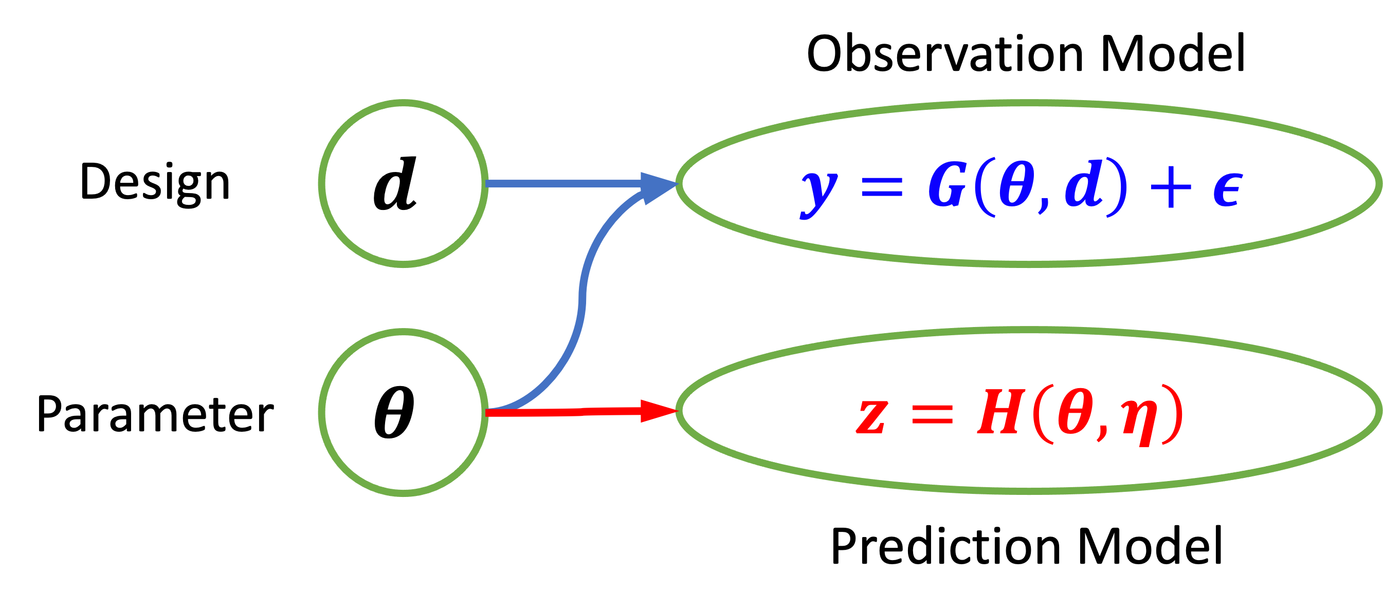
where is the vector of predictive QoIs that depends on the model parameters (but does not depend on the experimental design d) and prediction stochastic variable , and is a nonlinear stochastic prediction forward model (parameter-to-QoI mapping). Figure 1 illustrates the relationship of , y, d, and z through the observation and prediction models.
The prior-predictive and posterior-predictive PDFs for z are respectively
| (4) | ||||
| (5) |
If the prediction is deterministic (i.e., no prediction stochasticity ) then the respective PDFs are defined by pushforward probability measures under suitable conditions.555In situations where we can separate Eqn. 3 into deterministic and stochastic parts, e.g., , then we make the distinction between prior-/posterior-predictive and prior-/posterior-pushforward PDFs. “Predictive” refers to z, and “pushforward” refers to the deterministic prediction portion (e.g., ). The two names coincide when the prediction model is deterministic: . Whether stochastic or deterministic, we proceed with using z to denote the predictive QoIs.
We take a decision-theoretic approach [25] to quantify the value of an experiment. Let be the utility when y is obtained from an experiment performed at design d and the true data-generating parameters are . Since and y are unknown when designing the experiment, we take their joint expectation to arrive at the expected utility
| (6) |
In non-GO-OED, is typically chosen to be the KL divergence from the -prior to the -posterior. This leads to a that is equivalent to the MI between and y, or the EIG in [25]. Since GO-OED now targets the predictive QoIs z, we follow [4] and analogously employ the KL divergence from the z-prior-predictive to the z-posterior-predictive:
| (7) | ||||
| (8) |
Note that the utility itself, same as in the non-GO-OED case, does not dependent on . Substituting Eqn. 8 into Eqn. 6, we obtain
| (9) | ||||
| (10) |
which is the expected KL divergence (or EIG) on the predictive QoIs z (per Eqn. 9) and also the MI between y and z conditioned on d (per Eqn. 10). Notably, as stated by Theorem 1 in [4],
| (11) |
with equality if z is a one-to-one transformation of . That is, the EIG (or MI) on the predictive QoIs z is always less or equal than the EIG (or MI) on the parameters .
Lastly, solving the GO-OED problem entails finding the optimal design from a design space to maximize the expected utility:
| (12) |
3 Numerical Methods
3.1 Monte Carlo Estimation of the Expected Utility
In order to solve the GO-OED problem in Eqn. 12, we need to be able to evaluate . However, generally does not have a closed form and must be approximated numerically. We proceed to build a MC estimator for .
An initial MC estimator for Eqn. 9 may be written as
| (13) | ||||
| (14) |
where we can sample , (using observation model Eqn. 1), (using prediction model Eqn. 3). We do not explicitly have the prior-predictive PDF , but using MC samples we can estimate this density. However, we cannot evaluate the posterior-predictive PDF in the first term of Eqn. 14, nor can we directly estimate this conditional density from MC samples since we do not have multiple z samples for each . This motivates the following nested-loop MC estimator, continuing from Eqn. 13:
| (15) |
where and are respectively the number of samples for the outer and inner loops. For the first term, the outer loop is tasked with sampling , which is achieved by sampling followed by . The inner loop then samples and . For the second term, since is independent from both y and d, the term may be estimated separately from the above loops and from the optimization over d (i.e., omitted from the optimization statement in Eqn. 12). Here we write its estimation under the outer loop so to use the same samples to generate the prior-predictive samples, but noting that this is done only once at the beginning of the d optimization and need not be repeated at each d (see Algorithm 1).
The key of the nested-loop MC structure is that it allows multiple samples to be generated for each , and hence density estimation can be carried out for . Furthermore, while the prior, likelihood, and predictive sampling all can be done easily, is posterior sampling and non-trivial. In the next section, we discuss our approach to these two numerical challenges in the MC estimator for : posterior sampling and density estimation.
3.2 Posterior Sampling and Density Estimation
3.2.1 Markov Chain Monte Carlo for Sampling
We elect to perform posterior sampling via MCMC (see e.g., [1, 35, 5]), although the overall GO-OED framework is agnostic to the choice of posterior sampling method. MCMC will asymptotically sample the posterior distribution under sufficient conditions of ergodicity and detailed balance. In particular, we adopt an existing parallel Python MCMC implementation called emcee [15]. Emcee is built upon the affine invariant stretch move algorithm [17] that is designed to perform well under all linear transformations and therefore insensitive to correlation among parameters. The algorithm involves an ensemble of walkers . For the th walker currently at , the proposal procedure first randomly samples a among the current positions of the other walkers and then computes
| (16) |
where is drawn from a PDF satisfying in order to achieve the affine invariant property. For example [17] uses
| (19) |
where is an adjustable hyperparameter. Detailed balance is satisfied if the proposed point is accepted with probability
| (20) |
where the posterior density ratio can be calculated from just the prior and likelihood (marginal likelihood terms cancel out in the ratio). The emcee package further parallelizes the algorithm by splitting all walkers into two subsets, where walkers from within each subset are then updated by proposing from the other subset. The use of multiple walkers can potentially provide better exploration of multi-modal posteriors.
We note that in the GO-OED context, the posterior sampling is done conditioning on each sample, and we always have access to the true that generated this (see the sampling procedure described just below Eqn. 15). Hence, MCMC can be accelerated by initializing the walkers at , which corresponds to an “oracle estimator” that is generally much closer to the center region of the posterior than a randomly initialized point from the prior. Thus, MCMC in GO-OED is more benign, and requires fewer iterations, than a typical Bayesian inference problem. However, for unidentifiable and multi-modal posteriors, this technique is less effective and samplers suited for multi-modality may be more appropriate [13, 23, 33, 30, 10]. As with general MCMC, convergence diagnostics should be evaluated to make sure the choice of sampler and its parameters are amenable to the problem [12, 36].
3.2.2 Kernel Density Estimation for and
We perform density estimation for the prior- and posterior-predictive PDFs, respectively and , using KDE. Given samples , the estimated PDF from KDE is
| (21) |
where is the kernel and is its bandwidth matrix. We use the Scikit-Learn KDE implementation [31] that employs an isotropic Gaussian kernel with :
| (22) |
Thus, plays the role of standard deviation of the kernel, and smaller leads to sharper peaks around each sample while larger induces a more diffusive effect. Many methods for choosing exist [29, 9, 22] but they become expensive if needs to be repeated for with every sample and at each new d. In order to maintain a reasonable computational cost for bandwidth selection, at each d, we perform 5-fold cross-validation to select the optimal during the first few outer-loop iterations, and then choose the average value of those optimal ’s and fix it in all subsequent computations for that d. Bandwidth can certainly affect the estimation of , where too small of a bandwidth produces sharper posteriors and therefore higher perceived EIG and overestimate of , while too large a bandwidth tends to underestimate . We will explore the effects of KDE bandwidth in the numerical experiments.
3.3 Bayesian Optimization
Lastly, we need an optimization algorithm to solve Eqn. 12. Such algorithm needs to handle noisy objectives since only MC estimates of are available. Grid search may be feasible for low dimensional d (e.g., ) but the number of grid points grows exponentially with . While previous efforts have investigated derivative-free (e.g., nonlinear simplex and simultaneous perturbation stochastic approximation) [19] and gradient-based (e.g., Robbins-Monro and sample average approximation) [20] optimization methods in the context of non-GO-OED, the former can be slow in convergence and the latter requires gradient access and more prone to local optima.
We explore the use of BO in this work favoring its globally convergent properties, high sample efficiency and noise tolerance, and suitability for expensive objective function evaluations [32, 37, 16, 38]. In particular, we adopt the Nogueira Python BO package [28]. BO describes the objective function as a Gaussian process (GP) [34, 18], and its GP prior can be updated to a posterior analytically when new “observations” (i.e., evaluations) of become available. The next evaluation point for is then determined by optimizing a relevant acquisition function derived from the GP, which does not require gradient of . We summarize below the three main BO steps along with our choice of algorithm settings.
3.3.1 Step 1: Gaussian Process Regression
BO uses a GP to represent the uncertainty of a random function that we wish to optimize. The GP is specified by a mean function and covariance kernel . While different kernel choices are possible, we adopt the Matérn kernel [34], a popular choice that also generalizes the radial basis function:
| (23) |
where controls the smoothness, is the length scale, is the Euclidean distance, is the gamma function, and is the modified Bessel function. We further fix but re-tune the hyperparameter every time the GP is updated. As new evaluations of the random function at locations become available, the GP’s prior mean and covariance are updated to the posterior mean and covariance following standard GP regression update formulas [34].
3.3.2 Step 2: Acquisition Function
The selection of the next d to evaluate is guided by an acquisition function. Thus, the acquisition function needs to be inexpensive to evaluate and optimize, and reflects the potential value of a new evaluation towards the overall optimization problem in Eqn. 12. Many choices of acquisition function have been proposed in the BO literature, such as the upper confidence bound (UCB), probability of improvement (PI), and expected improvement (EI) (see, e.g., [21, 26, 40]). We select a simple 99.5% UCB in this work.
3.3.3 Step 3: Optimization Update
The next location to evaluate is then selected by maximizing the acquisition function. This inner optimization subproblem is inexpensive by design and needs not be solved very accurately in practice. We solve it using the limited-memory Broyden-Fletcher-Goldfarb-Shanno algorithm with box constraints (L-BFGS-B) [27][Ch. 7] and with multiple restarts. Upon obtaining , the GP can then be updated via Step 1. The cycle can be repeated until we reach a stopping criterion (e.g., maximum allowable iteration, lack of improvement to the highest value of encountered).
3.4 Summary of the Overall Algorithm
Pseudocode for our overall MCMC-based GO-OED algorithm is provided in Algorithm 1.
4 Numerical Experiments and Results
We present a series of numerical experiments with increasing complexity and designed to illuminate different aspects of the GO-OED approach. Section 4.1 starts with several cases with one-dimensional (1D) parameter, observation, and design spaces. The primary purposes of these examples are to validate GO-OED by comparing it with accessible and accurate non-GO-OED results under situations where theory shows they should agree, and to explore GO-OED’s numerical behavior (e.g., effect of KDE bandwidth). Section 4.2 increases to two-dimensional (2D) parameter, observation, and design spaces with a focus to present the effectiveness of BO. Lastly, Sec. 4.3 presents a problem of sensor placement in a convection-diffusion field with predictive QoIs that include future concentrations at various locations and flux across a boundary. The last problem involves even higher dimensional settings and provides illustrations that involves physics-based modeling.
4.1 1D Nonlinear Test Problems
We begin with a 1D test problem from [19] to explore some basic properties of our GO-OED approach. Consider a nonlinear observation model:
| (24) |
where all variables are scalar, , , and prior . With this observation model, below we present cases involving different combinations of prediction models.
Case Bn
First, we set up a benchmark (Bn) case where the prediction model is itself:
| (25) |
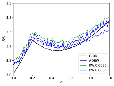
GO-OED therefore coincides with non-GO-OED and near-identical results are expected. As a high-accuracy reference solution, we estimate using a gridding method on a fine grid of 2000 nodes for discretizing the parameter space . The unnormalized posterior PDF (i.e., likelihood times prior) is calculated on this grid and then normalized by approximating the marginal likelihood through the mid-point integration rule. However, gridding is not scalable to higher dimensional and only implementable for prediction models of , therefore it is not be available for other test cases.
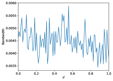
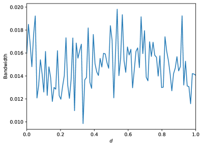
Figure 2a shows the expected utility computed using gridding (GRID), adaptive bandwidth (ADBW) (KDE bandwidth adaptively optimized at each using cross-validation as described in Sec. 3.2.2), and fixed bandwidth (BW) (KDE bandwidth fixed across all , illustrated at two pre-selected values) methods. MCMC used for ADBW and BW employed 1000 iterations with an additional 50 for burn-in. While all methods preserve the general trend in the expected utility, the discrepancies of ADBW and BW compared to the GRID reference is noticeable. Both ADBW and BW exhibit variance and bias, which result from the underlying MCMC and KDE computations. The optimized bandwidths for ADBW are shown in Fig. 2b across , varying roughly between and . As shown in Fig. 2a, the expected utility when setting BW to roughly ADBW’s lower (0.0035) and upper (0.006) bandwidth limits approximately creates an envelopes around the ADBW expected utility curve. This is consistent with the anticipated behavior described in Sec. 3.2.2, where a lower bandwidth tends to form narrower posterior distributions and overestimate the EIG, and vice versa for higher bandwidth. Overall, ADBW and BW perform similarly, suggesting that fixing bandwidth across the design space may be sufficient in practice.
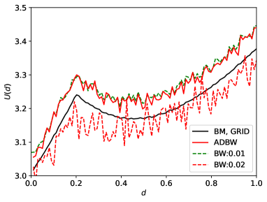
Case T1
In case T1, we adopt a nonlinear prediction model that differs from the observation model:
| (26) |
Since the prior for has compact support between , the predictive QoI is bijective for the parameter within this range. From Eqn. 11, a bijective parameter-to-observation mapping should lead to the same EIG as the non-GO-OED case just as in Case Bn. This is confirmed by the expected utility curves shown in Fig. 3a, all agreeing with the trend of the non-GO-OED GRID results in Case Bn (which is equivalent to this case). The GO-OED methods here, however, exhibit additional variance and bias from the KDE and MCMC compared to those in the Bn case. This is likely due to the increased sensitivity and variability of the mapping from to . The optimized bandwidths from ADBW is shown in Fig. 3b across , varying roughly between and . Similar to the previous case, in Fig. 3a we observe that the expected utility curves when setting BW to around ADBW’s lower (0.01) and upper (0.02) bandwidth limits create an envelope around ADBW, although the upper curve (from the lower bandwidth limit) is quite tight. Given the challenges in identifying a suitable fixed bandwidth a priori, we will focus on the ADBW for upcoming cases.
Case T2 and T3
In cases T2 and T3, we adopt observation models where is no longer bijective with . These illustrations will show that reducing the uncertainty of parameters is not equivalent to reducing the uncertainty of predictive QoI , leading to different optimal designs. Consider prediction model T2:
| (27) |
and prediction model T3:
| (28) |
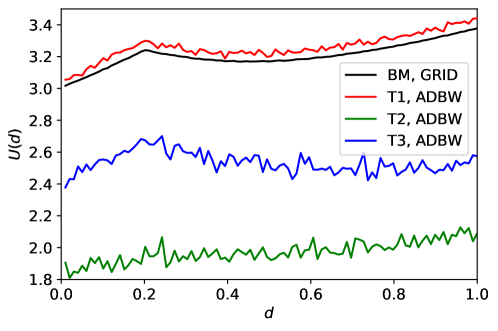
The expected utility curves for T2 and T3 are shown in Fig. 4, which are significantly different from that of Bn and T1. Notably, T2 continuously increases with roughly at a constant rate and reaches an optimal around , and T3 does not “tail up” as much as T1/Bn when approaches 1.0 while reaching an optimal around .
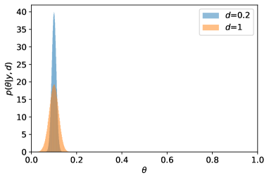
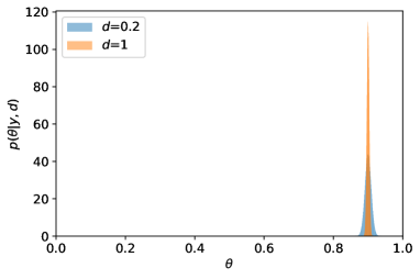
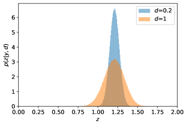
To further illuminate the optimal design behavior of non-GO-OED versus GO-OED, we produce in Fig. 5 example posterior distributions when (T3 GO-OED optimum) and (non-GO-OED optimum). These examples are demonstrated by conditioning on simulated at and for parameter variety (recall prior ). From Fig. 5a where the is simulated at , yields a narrower posterior (KL divergence from prior to posterior, or information gain, of 3.15) while offers a slightly wider posterior (information gain 2.44). Figure 5b presents another example for when is simulated at , where the opposite is observed (information gain 3.89 at is higher than information gain 3.23 at ). The variability in information gain thus can alter the ranking of the two designs. When this procedure is repeated for many samples of and and taking the expectation, it is the expected information gain on that becomes higher at than at .
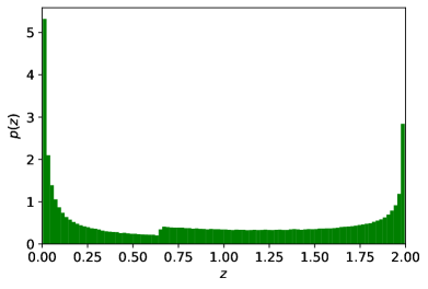
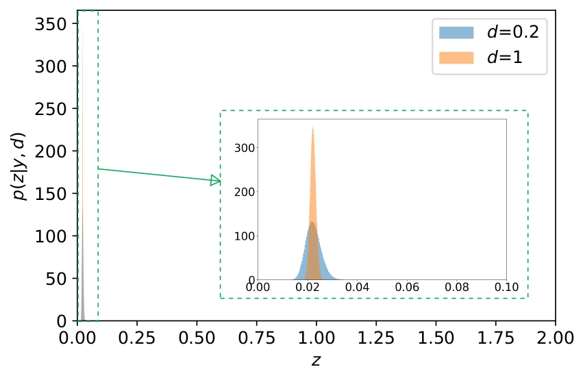
We perform the same assessment for the posterior-predictive distributions, shown in Fig. 6. To begin, we note that the prior-predictive, shown in Fig. 6a, is no longer uniform after is transformed through the T3 prediction model in Eqn. 28 but rather highly concentrated towards the two ends and slightly higher on the left side. The subsequent information gains on the QoIs will thus be computed relative to a KDE fit to this prior-predictive distribution. In Fig. 6b we see the case where is simulated at and design yields a narrower posterior-predictive (information gain 2.49) while design offers a slightly wider posterior-predictive (information gain 1.76). Figure 6c presents another example for when is simulated at , where again the opposite is observed (information gain 2.11 at is higher than information gain of 1.91 at ). First, we note that these information gain values are all lower than their information gain counterparts from Fig. 5; this is again consistent with the inequality in Eqn. 11. Second, the variability in information gain can again alter the ranking of the two designs. Upon taking the expected information gain over different , , and values leads to an overall higher EIG on at than at ; this ranking is inverted compared to that in the EIG.
4.2 2D Nonlinear Test Problems
Next, we present test problems that entail 2D parameter, observation, and design spaces. The first example modifies the observation model from Eqn. 24 to incorporate a 2D :
| (29) |
where now the prior becomes and all other settings remain the same. We consider two subcases with new prediction models:
| (Easom Eqn.) | (30) | ||||
| (Rosenbrock Eqn.) | (31) |
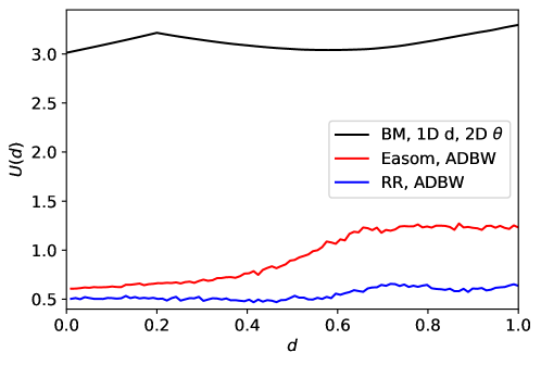
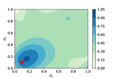
The non-GO-OED (via the gridding method) and GO-OED expected utilities are shown in Fig. 7. Both Easom and Rosenbrock subcases maximize EIG with a design around . To understand these results, we see that when is small is not easily identifiable, but as increases up to both and improve their identifiablilty, with ’s signal peaking at . As further increases, ’s identifiability continues to improve while ’s decreases again. This explains the trend of the non-GO-OED EIG curve in Fig. 7. However, the peak disappears for the EIG curves under the Easom and Rosenbrock prediction models. This can be understood from the forms of Eqn. 30 and 31. As noted above, for small information is only gained about and not . However, knowing alone does not provide much information about these QoIs without knowing some information about . When is larger we find more balanced information gain about both parameters alowing more information to be gained about these two functions.
Expanding further to 2D design and 2D observation spaces, the next case involves a multi-dimensional observation model:
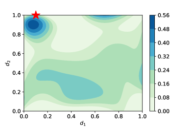
| (32) |
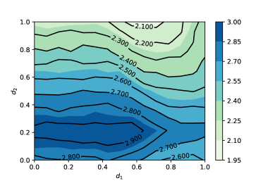
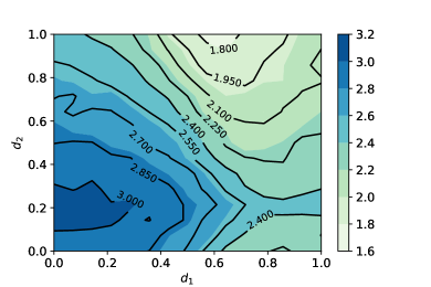
where . The prediction models are the same Easom and Rosenbrock equations from Eqn. 30 and Eqn. 31, respectively. The 2D GO-OED expected utility contours are shown in Fig. 8. In contrast to the 1D results in Fig. 7, the GO-OED contours now exhibit the local maximum at design values around 0.2. This is because the 2D observation model in Eqn. 32, through having both and pre-multiplying the two exponential terms, allows the learning of both parameters well at . As long as is small, the observation model means that both parameters are well identified so the QoIs will also be well identified.
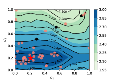
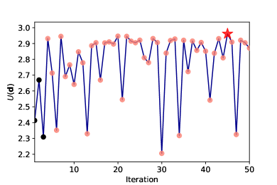
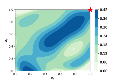
While the expected utility contours have all been constructed so far by estimating on a tensor grid of d, such brute-force grid search is computationally expensive and may only be done for low dimensional d. An optimization algorithm, such as the BO algorithm presented in Sec. 3.3, would be more efficient to seek out directly. Here we assess the BO performance in searching for the optimal design via the Easom prediction subcase. As seen in Fig. 9a, BO first randomly select 3 initial points (black) and then uses the UBC acquisition function to select the next points (in orange). We see these points cluster towards the eventual numerical optimum (red star) but maintains some exploration of the design space as well. The combination of exploitation and exploration can be seen further in Fig. 9b that plots the convergence history of BO. The values encountered in BO holds an overall increasing trend, but also scattered with low dips that are indicative of the occasional exploration. We will employ BO for all subsequent numerical demonstrations.
4.3 Convection-Diffusion Example
In this example, we apply GO-OED for the design of sensor locations in a 2D convection-diffusion field. In this scenario, the concentration (e.g., of a chemical contaminant) at location and time is governed by the convection-diffusion partial differential equation (PDE):
| (33) |
where is the (unknown) source location with a uniform prior , is the (known) convection velocity, and the source function has the form:
| (34) |
with and representing source strength and source width respectively. No-flux (homogeneous) Neumann boundary conditions are applied on all four boundaries of the square domain, and the initial condition is .
Numerical Solver and Surrogate Model
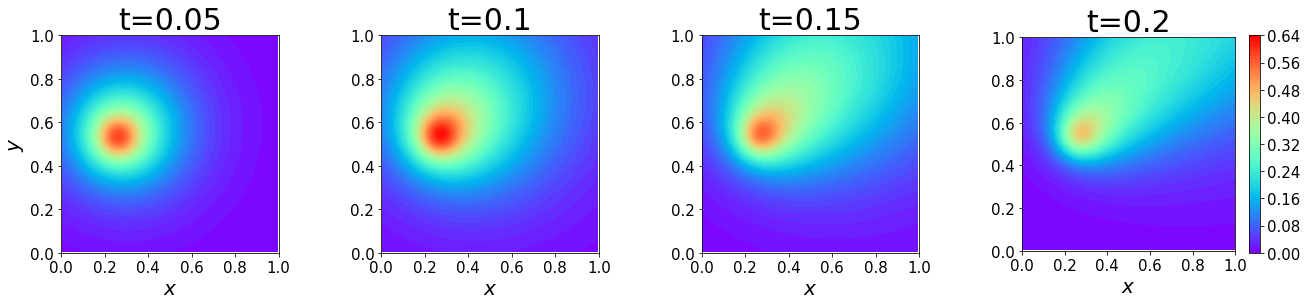
To numerically solve the PDE, we use second-order finite volume method on a uniform grid with , and the fractional step method for time marching with stepsize . The fractional step method combines an explicit second-order Adams–Bashforth discretization for the convective term and an implicit second-order Crank–Nicolson discretization for the diffusive term. Moreover, we employ the QUICK scheme [24] on the convective term to increase numerical stability. Example solutions of the concentration field at different time snapshots are shown in Fig. 10.
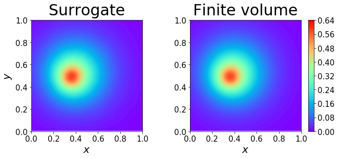
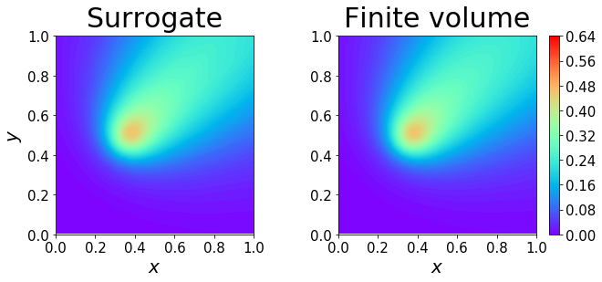
The OED cases (detailed setups to be presented later) will entail making observations at for predicting various QoIs at future time —hence, the concentrations and will be needed. While it is possible to directly use the finite volume forward model through the entire OED procedure, we construct deep neural network (DNN) surrogate models for quantities and in order to accelerate the computations. Each DNN has a four-dimensional input layer taking x and , five hidden layers with 40, 80, 40, 20 and 10 nodes, and a scalar output . To facilitate training of these surrogate models, finite volume solution fields are obtained at 2000 random samples drawn from the prior. The full dataset for the region of interest thus entails total points for , and also for . Each dataset is randomly shuffled and then divided to training and testing with an 80–20 split. Figure 11 provides comparisons of the the predicted concentration fields at and using DNN surrogates (left columns) and finite volume (right columns), which agree very well with testing mean-squared errors around and for and , respectively. More crucially, the DNN surrogates accelerate each forward model evaluation by about times compared to finite volume.
We begin by setting up an observation model for a design problem of selecting the coordinates of a single sensor at which the concentration can be observed:
| (35) |
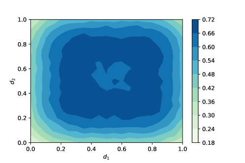
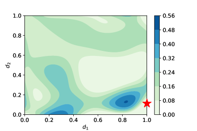
with . For a non-GO-OED that seeks to maximize the EIG on , the expected utility contour is shown in Fig. 12 where the optimal design appears around an inner ring roughly radius 0.2 from the center and slightly shifted to the top-right due to the convection direction to the top-right.
Future Concentration QoIs
For GO-OED, we first investigate when the predictive QoI is set to
| (36) |
with four subcases of (a) , (b) , (c) , and (d) . Each subcase corresponds to predicting the concentration near one of the four corners at future time . The expected utility contours for the subcases are shown in Fig. 13, which appear drastically different from the non-GO-OED result in Fig. 12. The regions of high expected utility roughly coincide with location of the predictive QoIs: for example, for subcase (a) where the QoI is in near the top-left corner, the GO-OED optimal design also follows towards the top-left. The more elongated contour for subcase (b) results from the convection in the top-right direction, where there is value in taking the earlier measurement at upstream of the targeted top-right at .
Next, we illustrate a few cases with multiple sensors and combinations of QoIs. Consider the GO-OED case where the concentration at two locations, and , are of interest:
| (37) |
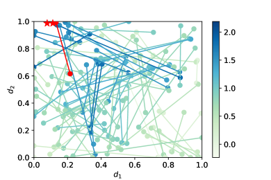
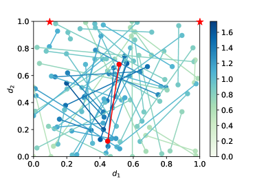
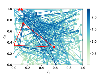
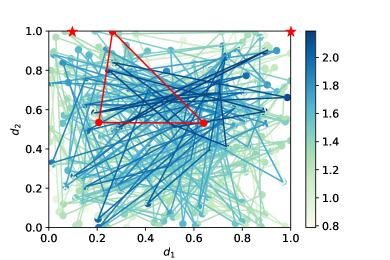
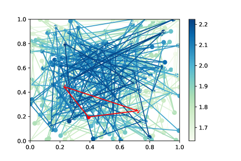
We consider two subcases of (a) and and (b) and . Figure 14 shows the sensor combinations encountered in BO (each combination is connected by a straight line) and the expected utility value is indicated by color intensity. The combination with the highest expected utility (i.e., the optimal 2-sensor design) is highlighted in red. In subcase (a), while both the QoI locations and are near the top-left corner, we see the sensor combinations with high expected utility tend to spread from top-left towards crossing the diagonal line of . Subcase (b) similarly does not simply place the two sensors near the locations. The high-value design patterns change further when designing for 3 sensors in Fig. 15, where now the optimal 3-sensor combination is connected by a triangle. Overall, the 3-sensor patterns appear more spread out, possibly as a result of having a larger number of observation opportunities. These observations suggest the non-trivial effects from the experiment dynamics and sensor coordination toward the experiment goals.
Future Flux QoI
Our final cases involve an QoI that is functional of the concentration field, namely the flux through the right boundary of the region of interest at . Such quantity is useful for understanding the total contaminant crossing the boundary into a sensitive or protected area to the right. The prediction model becomes
| (38) |
which we estimate using second-order center difference upon obtaining values from the DNN surrogate model. Figure 16 shows the 2-sensor combinations encountered in BO with the best combination highlighted in red. In general, combinations of top-left-to-bottom-right tend to provide higher EIG for this flux QoI, and the sensors are not simply placed geographically close to the flux being considered (i.e., close to the right boundary).
The last example illustrates a 3-sensor design while combining two different types of QoI together: the concentration at and the flux through the right boundary. Figure 17 shows the 3-sensor combinations encountered in BO with the best combination highlighted in red. We again observe a more spread-out pattern, likely due of having a larger number of observation opportunities.
5 Conclusions
We presented a computational method for Bayesian GO-OED that estimates and optimizes the EIG on the predictive QoIs under nonlinear observation and prediction models. This was achieve by establishing a nested MC estimator for the QoIs’ EIG, which used MCMC for the necessary posterior sampling. Posterior-predictive samples were then generated by propagating the posterior samples through the prediction model, and subsequently posterior-predictive PDF was approximated via KDE, finally allowing the KL divergence to be computed from the QoIs’ prior-predictive distribution to the posterior-predictive distribution. The GO-OED design was then found by maximizing the EIG estimate in the design space using BO.
A number of numerical experiments were provided to illuminate different aspects of the GO-OED framework. These included 1D test problems for validating GO-OED results against alternate computing methods, and exploring GO-OED’s numerical behavior (e.g., KDE bandwidth) in simple, controlled settings. 2D examples then followed to demonstrate the effectiveness of BO. Finally, a problem of sensor placement in a convection-diffusion field involving physics-based modeling was investigated to illustrate different predictive QoIs that included concentrations at various locations and flux across a boundary, all at a future time. Throughout these examples, we demonstrated that GO-OED and non-GO-OED design configuration may differ significantly.
A key limitations of this paper’s GO-OED is its dependence on MCMC and KDE. While MCMC can be accelerated by initializing the walkers from the true sample-generating parameter values, it can still be slow for complex posterior manifolds and high dimensional parameter spaces. This can introduce high estimator variance. KDE in principle converges to the true density as sample size increases, its finite approximation error can still greatly shift the optimal design locations. The adaptive tuning of bandwidth is also not infallible (i.e. still leading to bias), and becomes expensive if re-tuning is required frequently (e.g., for every MC sample). Promising directions of future work thus entail seeking more efficient methods for estimating the EIG, for example through more sophisticated density estimations such as Gaussian mixture models, transport maps, and normalizing flows; deriving and optimizing bounds for EIG; and building density ratio estimators that can also accommodate implicit likelihood situations.
Acknowledgments
WS, TC, and XH are supported in part by the U.S. Department of Energy, Office of Science, Office of Office of Advanced Scientific Computing Research under Award Number DE-SC0021397. Sandia National Laboratories is a multimission laboratory managed and operated by National Technology and Engineering Solutions of Sandia, LLC, a wholly owned subsidiary of Honeywell International, Inc., for the U.S. Department of Energy’s National Nuclear Security Administration under contract DE-NA-0003525. This paper describes objective technical results and analysis. Any subjective views or opinions that might be expressed in the paper do not necessarily represent the views of the U.S. Department of Energy or the United States Government.
References
- [1] C. Andrieu, N. de Freitas, A. Doucet, and M. I. Jordan. An Introduction to MCMC for Machine Learning. Machine Learning, 50:5–43, 2003.
- [2] A. C. Atkinson, A. N. Donev, and R. D. Tobias. Optimum Experimental Designs, With SAS. Oxford University Press, New York, NY, 2007.
- [3] A. Attia, A. Alexanderian, and A. K. Saibaba. Goal-oriented optimal design of experiments for large-scale Bayesian linear inverse problems. Inverse Problems, 34(9):aad210, 2018.
- [4] J. M. Bernardo. Expected Information as Expected Utility. The Annals of Statistics, 7(3):686–690, 1979.
- [5] S. Brooks, A. Gelman, G. Jones, and X.-L. Meng, editors. Handbook of Markov Chain Monte Carlo. Chapman and Hall/CRC, 2011.
- [6] T. Butler, J. Jakeman, and T. Wildey. Combining Push-Forward Measures and Bayes’ Rule to Construct Consistent Solutions to Stochastic Inverse Problems. SIAM Journal on Scientific Computing, 40(2):A984–A1011, 2018.
- [7] T. Butler, J. Jakeman, and T. Wildey. Convergence of Probability Densities Using Approximate Models for Forward and Inverse Problems in Uncertainty Quantification. SIAM Journal on Scientific Computing, 40(5):A3523–A3548, 2018.
- [8] T. Butler, J. D. Jakeman, and T. Wildey. Optimal experimental design for prediction based on push-forward probability measures. Journal of Computational Physics, 416:109518, 2020.
- [9] R. Cao, A. Cuevas, and W. González Manteiga. A comparative study of several smoothing methods in density estimation. Computational Statistics & Data Analysis, 17(2):153–176, 1994.
- [10] T. A. Catanach and J. L. Beck. Bayesian updating and uncertainty quantification using sequential tempered MCMC with the rank-one modified Metropolis algorithm. arXiv preprint arXiv:1804.08738, 2018.
- [11] K. Chaloner and I. Verdinelli. Bayesian Experimental Design: A Review. Statistical Science, 10(3):273–304, 1995.
- [12] M. K. Cowles and B. P. Carlin. Markov chain Monte Carlo convergence diagnostics: a comparative review. Journal of the American Statistical Association, 91(434):883–904, 1996.
- [13] D. J. Earl and M. W. Deem. Parallel tempering: Theory, applications, and new perspectives. Physical Chemistry Chemical Physics, 7(23):3910–3916, 2005.
- [14] V. V. Fedorov. Theory of Optimal Experiments. Academic Press, New York, NY, 1972.
- [15] D. Foreman-Mackey, D. W. Hogg, D. Lang, and J. Goodman. emcee: The MCMC Hammer. Publications of the Astronomical Society of the Pacific, 125(925):306–312, 2013.
- [16] P. I. Frazier. A tutorial on Bayesian optimization. arXiv preprint arXiv:1807.02811, 2018.
- [17] J. Goodman and J. Weare. Ensemble samplers with affine invariance. Communications in Applied Mathematics and Computational Science, 5(1):65–80, 2010.
- [18] R. B. Gramacy. Surrogates. Chapman and Hall/CRC, mar 2020.
- [19] X. Huan and Y. M. Marzouk. Simulation-based optimal Bayesian experimental design for nonlinear systems. Journal of Computational Physics, 232(1):288–317, 2013.
- [20] X. Huan and Y. M. Marzouk. Gradient-Based Stochastic Optimization Methods in Bayesian Experimental Design. International Journal for Uncertainty Quantification, 4(6):479–510, 2014.
- [21] D. R. Jones, M. Schonlau, and W. J. Welch. Efficient global optimization of expensive black-box functions. Journal of Global Optimization, 13:455–492, 1998.
- [22] M. C. Jones, J. S. Marron, and S. J. Sheather. A Brief Survey of Bandwidth Selection for Density Estimation. Journal of the American Statistical Association, 91(433):401–407, 1996.
- [23] J. Latz, J. P. Madrigal-Cianci, F. Nobile, and R. Tempone. Generalized parallel tempering on Bayesian inverse problems. Statistics and Computing, 31(5):67, 2021.
- [24] B. Leonard. A stable and accurate convective modelling procedure based on quadratic upstream interpolation. Computer Methods in Applied Mechanics and Engineering, 19(1):59–98, jun 1979.
- [25] D. V. Lindley. On a Measure of the Information Provided by an Experiment. The Annals of Mathematical Statistics, 27(4):986–1005, 1956.
- [26] J. Močkus. On Bayesian methods for seeking the extremum. In Optimization Techniques IFIP Technical Conference, pages 400–404, 1975.
- [27] J. Nocedal and S. J. Wright. Numerical Optimization. Springer New York, New York, NY, 2006.
- [28] F. Nogueira. Bayesian Optimization: Open source constrained global optimization tool for Python, 2014.
- [29] B. U. Park and J. S. Marron. Comparison of data-driven bandwidth selectors. Journal of the American Statistical Association, 85(409):66–72, 1990.
- [30] D. Paulin, A. Jasra, and A. Thiery. Error bounds for sequential Monte Carlo samplers for multimodal distributions. and Probability, 25(1):310–340, 2019.
- [31] F. Pedregosa, G. Varoquaux, A. Gramfort, V. Michel, B. Thirion, O. Grisel, M. Blondel, P. Prettenhofer, R. Weiss, V. Dubourg, J. Vanderplas, A. Passos, D. Cournapeau, M. Brucher, M. Perrot, and E. Duchesnay. Scikit-learn: Machine learning in Python. Journal of Machine Learning Research, 12:2825–2830, 2011.
- [32] M. Pelikan, D. E. Goldberg, and E. Cantú-Paz. BOA: The Bayesian Optimization Algorithm. In Proceedings of the 1st Annual Conference on Genetic and Evolutionary Computation - Volume 1, GECCO’99, page 525–532, 1999.
- [33] E. Pompe, C. Holmes, and K. Łatuszyński. A Framework for Adaptive MCMC Targeting Multimodal Distributions. arXiv preprint arXiv:1812.02609, 2018.
- [34] C. E. Rasmussen and C. K. I. Williams. Gaussian Processes for Machine Learning. The MIT Press, Cambridge, MA, 2006.
- [35] C. P. Robert and G. Casella. Monte Carlo Statistical Methods. Springer New York, New York, NY, 2004.
- [36] V. Roy. Convergence diagnostics for Markov chain Monte Carlo. Annual Review of Statistics and Its Application, 7:387–412, 2020.
- [37] B. Shahriari, K. Swersky, Z. Wang, R. P. Adams, and N. de Freitas. Taking the Human Out of the Loop: A Review of Bayesian Optimization. Proceedings of the IEEE, 104(1):148–175, 2016.
- [38] X. Wang, Y. Jin, S. Schmitt, and M. Olhofer. Recent advances in Bayesian optimization. ACM Computing Surveys, 55(13s):1–36, 2023.
- [39] K. Wu, P. Chen, and O. Ghattas. An efficient method for goal-oriented linear Bayesian optimal experimental design: Application to optimal sensor placement. arXiv preprint arXiv:2102.06627, 2021.
- [40] D. Zhan and H. Xing. Expected improvement for expensive optimization: a review. Journal of Global Optimization, 78(3):507–544, 2020.