From Sontag’s to Cardano-Lyapunov Formula for Systems
Not Affine in the Control: Convection-Enabled PDE Stabilization

Abstract

We propose the first generalization of Sontag’s universal controller to systems not affine in the control, particularly, to PDEs with boundary actuation. We assume that the system admits a control Lyapunov function (CLF) whose derivative, rather than being affine in the control, has either a depressed cubic, quadratic, or depressed quartic dependence on the control. For each case, a continuous universal controller that vanishes at the origin and achieves global exponential stability is derived. We prove our result in the context of convection-reaction-diffusion PDEs with Dirichlet actuation. We show that if the convection has a certain structure, then the $L^{2}$ norm of the state is a CLF. In addition to generalizing Sontag’s formula to some non-affine systems, we present the first general Lyapunov approach for boundary control of nonlinear PDEs. We illustrate our results via a numerical example.

I Introduction and Main Result

I-A Sontag’s formula

Artstein considers in his 1983 paper [1] the problem of smooth stabilization of control systems

$$\dot{u}=f(u,v),$$ (1)

where, for consistency with the notation used in PDE control, $u$ denotes the state, $v$ denotes the control input, and $f$ a smooth vector field. One of Artstein’s results is that, if the system admits a smooth CLF, then there exists a stabilizing feedback $v(u)$ with $v(0)=0$, which is smooth everywhere except possibly at the origin $u=0$. If the system possesses the ‘small control property,’ then continuity at the origin can be guaranteed.

Artstein’s proof is not constructive: the feedback is not designed. For systems affine in the control,

$$\dot{u}=f(u)+g(u)v,$$ (2)

where $f$ and $g$ are smooth, Sontag provides a feedback formula in his 1989 paper [2]. Among various pedagogical presentations of Sontag’s universal controller, the reader may consult Section 1.3 in [3].

Extensions of Sontag’s formula are too numerous to comprehensively survey. For example, in [4], a bounded version of Sontag’s controller is proposed under the assumption that the system admits a CLF whose derivative can be made negative by choosing the control input $v$ in a bounded set. In [5, equation (2.4)], the concept of adaptive CLF is introduced for stabilization of nonlinear systems, linear in the unknown constant parameters, and an “adaptive Sontag’s formula” is given. The extension of Sontag’s formula to systems affine in a deterministic disturbance is given in [6, equation (35)]. Sontag’s formula for stochastic systems is introduced in [7, equation (5.12)]. In [8], Sontag’s formula is generalized to the case where the input is affected by a disturbance, to guarantee integral-input-to-state stability. Finally, in [9], Sontag’s formula is adapted for the problem of event-based stabilization of control-affine systems.

I-B Going beyond control-affine systems: Framework

None of the results above go beyond the control-affine case. Our first contribution here is to take the construction of a universal feedback controller beyond the control-affine case, motivated by classes of boundary-actuated PDEs. Specifically, the question we ask, a third of a century after [2], is: Given a CLF $V$ for a control system (not necessarily finite-dimensional), for which $\dot{V}$ is not affine in the control $v$, can we construct a ’universal’ feedback controller $v$ that vanishes at the origin, is at least ’continuous everywhere’, and stabilizes the existing solutions? In other words, can we extend the universal control concept beyond the control-affine case?

To answer the above question, we consider the class of scalar-valued PDE systems admitting a CLF $V$, whose time derivative has a polynomial structure in the control input $v$, i.e.,

$$\dot{V}(u)\leq\phi(u)+\gamma(v,u),$$ (3)

where $\phi$ is some operator acting on the state $u$ that verifies $\phi(0)=0$ and such that $\phi(u)$ does not depend explicitly on $v$, and $\gamma(v,u)$ is a polynomial in the control input $v$, whose higher-order coefficient is constant, and whose lower-order coefficients may depend on $u$ but not on $v$.

The inspiration for this work comes from [10], [11], [12], [13], and [14]. In [10], stabilization of the inviscid Burgers’ equation is achieved by exploiting the quadratic convection $-(u^{2})_{x}$, which makes $\dot{V}$ cubic in the control, with $V$ being the $L^{2}$ norm of the state. In [11], [12], and [13], it is shown that the $L^{2}$ norm of the state of the Kuramoto-Sivashinsky is a CLF, because of the convection $-(u^{2})_{x}$. Stabilization is then achieved. In [14], the authors consider a reaction-diffusion PDE, observe that a spatially weighted $L^{2}$ norm of the state is quadratic in the control, thanks to the diffusion term, and propose a stabilizing feedback, which is a root of a quadratic equation.

We consider the following structures for $\gamma$:

$$\gamma(v,u):=\pm v^{3}+\beta(u)v\quad$$ (depressed cubic), (4)

$$\gamma(v,u):=-v^{2}+\beta(u)v\quad$$ (quadratic), (5)

$$\gamma(v,u):=-v^{4}+\beta(u)v\quad$$ (depressed quartic), (6)

where $\beta$ is some continuous operator acting on $u$ that verifies $\beta(0)=0$. For each structure on $\gamma(v,u)$, we construct a universal continuous feedback

$$v\left(V(u),\beta(u),\phi(u)\right)$$ (7)

that verifies $v(0)=0$ and, under which, the regular closed-loop solutions verify

$$\dot{V}(u)\leq-\alpha(V(u))\,,\quad\alpha\in{\cal K}\,,$$ (8)

where $\alpha\in\mathcal{K}$ if $\alpha$ is continuous, strictly increasing and $\alpha(0)=0$. For example, one can choose $\alpha(V):=V$ to enforce exponential stability. The controller (7) is said to be universal because its structure is not specific to $\phi(u)$ and $\beta(u)$, which are general/universal. The structure of the controller depends only on the structure of the actuated part of the CLF, i.e. $\gamma(v,u)$.

The universal feedback (7), when $\gamma(v,u)$ has the cubic structure (4); namely, when

$$\dot{V}\leq\phi+\beta v\pm v^{3}\,,$$ (9)

is given by what we suggest to be called the Cardano-Lyapunov formula

$$\framebox{$\displaystyle v:=\sqrt[3]{-\frac{q}{2}+\sqrt{\frac{q^{2}}{4}\pm\frac{\beta^{3}}{27}}}+\sqrt[3]{-\frac{q}{2}-\sqrt{\frac{q^{2}}{4}\pm\frac{\beta^{3}}{27}}}$}$$ (10)

where

$$\framebox{$\displaystyle q:=~{}\pm\left[|\phi(u)|+\frac{2\sqrt{3}}{9}|\beta(u)|^{\frac{3}{2}}+\alpha(V(u))\right]$}$$ (11)

Note that, unlike the classical control-affine case, $\dot{V}=L_{f}V+L_{g}Vv$, where one has to assume that $L_{g}V=0\Rightarrow L_{f}V<0$, in (9) the cubic term $\pm v^{3}$ removes the need for any assumptions on $\phi$ and $\beta$—namely, $V$ is a CLF by virtue of (9) alone.

I-C Going beyond control-affine systems: Motivation

We illustrate our result on the class of scalar convection-reaction-diffusion (CRD) PDEs of the form

$$u_{t}=\epsilon u_{xx}+C(u)_{x}+R(u)\,\qquad x\in(0,1),$$ (12)

where $R(u)$ is the reaction which is continuous and verifies $R(0)=0$; $C(u)_{x}$ is the convection; and $\epsilon u_{xx}$ is the diffusion with $\epsilon>0$. We suppose that this system is subject to the Dirichlet actuation

$$u(0)=v,$$ (13)

$$u(1)=0,$$ (14)

in which $v$ is the control input to be designed to stabilize the origin $u:=0$ of (12) in the $L^{2}$ sense. Three types of convection are considered; namely,

$$C(u)_{x}:=\pm(u^{2})_{x}\quad$$ (flow convection), (15)

$$C(u)_{x}:=u_{x}\quad$$ (counter-convection), (16)

$$C(u)_{x}:=(u^{3})_{x}\quad$$ (Buckmaster convection). (17)

We reveal that the $L^{2}$ norm

$$V(u):=\frac{1}{2}\int_{0}^{1}u(x)^{2}dx$$ (18)

is a CLF for the control system (12), under (13), (14), if the convection is given by (15), (16), or (17). In particular, $\dot{V}$ is not affine in the control input $v$ and satisfies (3), with $\gamma(v,u)$ a depressed cubic in the case of flow convection; quadratic in the case of counter-convection; and depressed quartic in the case of Buckmaster convection. The function $\phi(u)$ in (3) depends only on the reaction and the diffusion, while the function $\beta(u)$ in (4), (5) and (6) comes only from the diffusion.

CRD PDEs are difficult to control because of the reaction, which is the main source of instability. An example of a CRD PDE that is difficult to stabilize is

$$u_{t}=\epsilon u_{xx}-(u^{2})_{x}+\lambda u^{3}$$ (19)

where $\lambda>0$ is constant. The superlinear reaction $u^{3}$ contributes to blow-up type phenomena in open-loop and may lead to the lack of global controllability [15, 16, 17]. Add to that, standard approaches such as linear backstepping cannot be applied to this system. For some PDEs involving superlinear reaction terms, it is possible to use nonlinear backstepping [18, 19, 20], but the resulting controller is extremely complex. It involves infinite Volterra series and the analysis of PDEs satisfied by the Volterra kernels, that evolve on Goursat domains. The dimension of the domains increases to infinity but the volume decreases to zero.

I-D Main result

For each case of the convection term $C(u)_{x}$, we design a feedback controller that achieves stabilization in the sense of inequality (8). Note that our approach is not limited to the CRD PDEs. It can be easily adapted to any control system that admits a CLF whose derivative verifies (3), under one of the structures (4), (5), or (6).

Theorem 1

Consider the control system (12), (13), (14), along with $V$ defined in (18). For each of the convection terms in (15), (16), and (17), there exists a continuous feedback

$$v\left(V,u_{x}(0),\int_{0}^{1}\left(u(x)R(u(x))-\epsilon u_{x}(x)^{2}\right)dx\right),$$ (20)

with the property $v(0)=0$ and guaranteeing that (8) holds for the closed-loop regular solutions. $\square$

The rest of the paper is devoted to the proof of Theorem 1, i.e. to the construction of the feedback (20). The universal controllers that we construct in this paper are remarkably simple in comparison with nonlinear backstepping controllers, as they are constructed using only finite number of additions, multiplications, and extraction of $n^{\rm th}$ roots. Hence, our result not only generalizes Sontag formula to non-affine cases, but also introduces a new method for boundary control of PDEs, distinct from PDE backstepping. We just need the PDE to possess a helpful convective structure.

II Construction of the Universal Controllers

In this section, we provide a constructive proof of Theorem 1, i.e. we design the feedback (20). The proof follows in two steps. First, we differentiate the Lyapunov function candidate $V$ along the regular solutions of (12), (13), (14). We obtain, on $\dot{V}$, a structure that is not affine in the control, in the form of (3). Then, we consider the cases of flow convection $\pm(u^{2})_{x}$, counter-convection $u_{x}$, and Buckmaster convection $(u^{3})_{x}$. We show that the flow convection leads to a depressed cubic structure on the control input $v$, the counter-convection leads to a quadratic structure, and that the Buckmaster convection leads to a depressed quartic structure. In each case, we construct the corresponding universal controller.

II-A Upperbounding $\dot{V}$

By differentiating $V$ along the regular solutions of (12), (13), (14), we find

$$\dot{V}= ~{}\int_{0}^{1}u(x)C(u(x))_{x}dx+\int_{0}^{1}u(x)R(u(x))dx$$

$$~{}+\epsilon\int_{0}^{1}u(x)u_{xx}(x)dx.$$ (21)

Using integration by parts and the boundary conditions (13), (14), we obtain

$$\dot{V}=-vC(v)-\int_{0}^{1}u_{x}(x)C(u(x))dx-\epsilon vu_{x}(0)$$

$$~{}-\epsilon\int_{0}^{1}u_{x}(x)^{2}dx+\int_{0}^{1}u(x)R(u(x))dx.$$ (22)

Next, we perform the change of variable $s:=u$, leading to $ds=u_{x}dx$. Equation (22) can therefore be rewritten as

$$\dot{V}= ~{}-vC(v)+\int_{0}^{v}C(s)ds-\epsilon\int_{0}^{1}u_{x}(x)^{2}dx$$

$$~{}+\int_{0}^{1}u(x)R(u(x))dx-\epsilon vu_{x}(0).$$ (23)

II-B Flow Convection

We distinguish between two cases. Either $C(u):=u^{2}$, or $C(u):=-u^{2}$. Let us start with a $C(u):=u^{2}$. Note that

$$-vC(v)+\int_{0}^{v}C(s)ds= ~{}-\frac{2}{3}v^{3}.$$ (24)

As a consequence, equation (23) becomes

$$\dot{V}= ~{}\int_{0}^{1}u(x)R(u(x))dx-\epsilon\int_{0}^{1}u_{x}(x)^{2}dx$$

$$~{}-\frac{2}{3}v^{3}-\epsilon vu_{x}(0).$$ (25)

The function $\dot{V}$ has a depressed cubic structure on the control input $v$. The first idea to enforce (8) is, therefore, to set $v$ as a real root of the cubic equation

$$0=v^{3}+\frac{3\epsilon}{2}vu_{x}(0)$$

$$~{}-\frac{3}{2}\left(\alpha(V)+\int_{0}^{1}\left(u(x)R(u(x))-\epsilon u_{x}(x)^{2}\right)dx\right).$$ (26)

Selecting arbitrarily one real root of (26) at each time instant may lead to $v$ being discontinuous with respect to the coefficients of (26). We need more work to enforce the continuity of $v$. This being said, we propose to consider instead the cubic equation

$$0= ~{}v^{3}+\frac{3\epsilon}{2}u_{x}(0)v-\frac{3}{2}\bigg{(}\alpha(V)+\frac{\sqrt{2\epsilon^{3}}}{3}|u_{x}(0)|^{\frac{3}{2}}$$

$$~{}+\bigg{|}\int_{0}^{1}\left(u(x)R(u(x))-\epsilon u_{x}(x)^{2}\right)dx\bigg{|}\bigg{)}.$$ (27)

If $v$ is a real root of (27), then we obtain

$$\dot{V}\leq ~{}-\alpha(V)-\frac{\sqrt{2\epsilon^{3}}}{3}|u_{x}(0)|^{\frac{3}{2}}$$

$$~{}+\int_{0}^{1}\left(u(x)R(u(x))-\epsilon u_{x}(x)^{2}\right)dx$$

$$~{}-\bigg{|}\int_{0}^{1}\left(u(x)R(u(x))-\epsilon u_{x}(x)^{2}\right)dx\bigg{|},$$ (28)

which implies (8). It remains to choose the real root $v$ of (27) such that it is continuous with respect to the coefficients of (27). To do so, we just need to remark that contrarily to (26), the depressed cubic equation (27) always admits a real root, which is given by Cardano formula, which is a continuous expression relating the coefficients of (27). This is due to the fact that the discriminant of (27) is nonnegative. Indeed, the discriminant of (27) is $\Delta:=q^{2}/4+\beta^{3}/27$, where $\beta$ and $q$ are given by

$$\beta:= ~{}\frac{3\epsilon}{2}u_{x}(0),$$ (29)

$$q:= ~{}-\frac{3}{2}\bigg{(}\alpha(V)+\bigg{|}\int_{0}^{1}\left(uR(u)-\epsilon u_{x}^{2}\right)dx\bigg{|}\bigg{)}$$

$$~{}-\frac{\sqrt{2\epsilon^{3}}}{2}|u_{x}(0)|^{\frac{3}{2}}.$$ (30)

Note that

$$q= ~{}-\frac{3}{2}\bigg{(}\alpha(V)+\bigg{|}\int_{0}^{1}\left(uR(u)-\epsilon u_{x}^{2}\right)dx\bigg{|}\bigg{)}$$

$$~{}-\frac{2\sqrt{3}}{9}|\beta|^{\frac{3}{2}}.$$ (31)

A direct computation gives us

$$\Delta= ~{}\frac{1}{4}\bigg{(}\frac{9}{4}\bigg{(}\alpha(V)+\bigg{|}\int_{0}^{1}\left(uR(u)-\epsilon u_{x}^{2}\right)dx\bigg{|}\bigg{)}^{2}$$

$$~{}+\frac{\sqrt{3}}{3}\bigg{(}\alpha(V)+\bigg{|}\int_{0}^{1}\left(uR(u)-\epsilon u_{x}^{2}\right)dx\bigg{|}\bigg{)}$$

$$~{}|\beta|^{\frac{3}{2}}+\frac{4}{27}|\beta|^{3}\bigg{)}+\frac{\beta^{3}}{27}\geq\frac{1}{27}(|\beta|^{3}+\beta^{3})\geq 0.$$ (32)

We, therefore, propose to set the control input $v$ as

$$v:=\sqrt[3]{-\frac{q}{2}+\sqrt{\frac{q^{2}}{4}+\frac{\beta^{3}}{27}}}+\sqrt[3]{-\frac{q}{2}-\sqrt{\frac{q^{2}}{4}+\frac{\beta^{3}}{27}}}.$$ (33)

This control input vanishes if the state vanishes. Indeed, if $u=0$, then $\beta=q=0$, which implies that $v=0$.

Considering now a negative convection, we obtain

$$-vC(v)+\int_{0}^{v}C(s)ds= ~{}\frac{2}{3}v^{3}.$$ (34)

As a consequence, equation (23) becomes

$$\dot{V}= ~{}\int_{0}^{1}u(x)R(u(x))dx-\epsilon\int_{0}^{1}u_{x}(x)^{2}dx$$

$$~{}+\frac{2}{3}v^{3}-\epsilon vu_{x}(0).$$ (35)

To enforce inequality (8), we consider the cubic equation

$$0= ~{}v^{3}-\frac{3}{2}\epsilon u_{x}(0)v+\frac{3}{2}\bigg{(}\alpha(V)+\frac{\sqrt{2\epsilon^{3}}}{3}|u_{x}(0)|^{\frac{3}{2}}$$

$$~{}+\bigg{|}\int_{0}^{1}\left(u(x)R(u(x))-\epsilon u_{x}(x)^{2}\right)dx\bigg{|}\bigg{)}.$$ (36)

The discriminant of (36) is $\Delta:=q^{2}/4+\beta^{3}/27$ with $\beta$ and $q$ defined as

$$\beta:= ~{}-\frac{3\epsilon}{2}u_{x}(0),$$ (37)

$$q:= ~{}\frac{3}{2}\bigg{(}\alpha(V)+\bigg{|}\int_{0}^{1}\left(uR(u)-\epsilon u_{x}^{2}\right)dx\bigg{|}\bigg{)}$$

$$~{}+\frac{\sqrt{2\epsilon^{3}}}{2}|u_{x}(0)|^{\frac{3}{2}}.$$ (38)

Since $\Delta\geq 0$, then we propose to set the control input $v$ as in (33). As previously, if $u=0$ then $\beta=q=0$ which leads to $v=0$.

II-C Counter-convection

In this case, we have

$$-vC(v)+\int_{0}^{v}C(s)ds= ~{}-\frac{1}{2}v^{2}.$$ (39)

As a result, equation (23) becomes

$$\dot{V}= ~{}\int_{0}^{1}u(x)R(u(x))dx-\epsilon\int_{0}^{1}u_{x}(x)^{2}dx$$

$$~{}-\frac{1}{2}v^{2}-\epsilon vu_{x}(0).$$ (40)

The function $\dot{V}$ has a quadratic structure in $v$. The first idea to enforce (8), is to set $v$ as a real root of the quadratic equation

$$0= ~{}\int_{0}^{1}\left(u(x)R(u(x))-\epsilon u_{x}(x)^{2}\right)dx$$

$$~{}-\frac{1}{2}v^{2}-\epsilon u_{x}(0)v+\alpha(V).$$ (41)

However, there is no guarantee that (41) admits a real root. We need to construct another polynomial equation as in the previous case. This being said, we consider the quadratic equation

$$0= ~{}\bigg{|}\int_{0}^{1}\left(u(x)R(u(x))-\epsilon u_{x}(x)^{2}\right)dx\bigg{|}$$

$$~{}-\frac{1}{2}v^{2}-\epsilon u_{x}(0)v+\alpha(V).$$ (42)

If $v$ is a real root of (42), then (8) is verified. The polynomial equation (42) admits either one double real root or two distinct real roots. This is due to the fact that its discriminant is nonnegative. Indeed, the discriminant of (42) is $\Delta:=b^{2}-4ac$, where $a$, $b$ and $c$ are given by

$$a:=-\frac{1}{2},\quad b:=-\epsilon u_{x}(0),$$ (43)

$$c:=\alpha(V)+\bigg{|}\int_{0}^{1}\left(uR(u)-\epsilon u_{x}^{2}\right)dx\bigg{|}.$$ (44)

Hence, $\Delta\geq 0$. We set then the control input $v$ as

$$v:=b\pm\sqrt{b^{2}+2c}.$$ (45)

If $u=0$ then $b=c=0$ which implies that $v=0$.

II-D Buckmaster Convection

The convection $(u^{3})_{x}$ is characteristic of the Buckmaster equation [21]. We have

$$-vC(v)+\int_{0}^{v}C(s)ds= ~{}-\frac{3}{4}v^{4}.$$ (46)

As a consequence, equation (23) becomes

$$\dot{V}= ~{}\int_{0}^{1}u(x)R(u(x))dx-\epsilon\int_{0}^{1}u_{x}(x)^{2}dx$$

$$~{}-\frac{3}{4}v^{4}-\epsilon vu_{x}(0).$$ (47)

The function $\dot{V}$ has a depressed quartic structure on $v$. The idea is to transform this depressed quartic structure into a biquadratic structure. Namely, using Young inequality, we find

$$-\epsilon vu_{x}(0)\leq ~{}\epsilon|v|\sqrt{|u_{x}(0)|}\sqrt{|u_{x}(0|}$$

$$\leq ~{}\frac{1}{2}|u_{x}(0)|v^{2}+\frac{\epsilon^{2}}{2}|u_{x}(0)|.$$ (48)

Equation (47) becomes

$$\dot{V}\leq ~{}\int_{0}^{1}u(x)R(u(x))dx-\epsilon\int_{0}^{1}u_{x}(x)^{2}dx$$

$$~{}-\frac{3}{4}v^{4}+\frac{1}{2}|u_{x}(0)|v^{2}+\frac{\epsilon^{2}}{2}|u_{x}(0)|.$$ (49)

The function $\dot{V}$ has a biquadratic structure in $v$. We perform the change of variable $\tilde{v}:=v^{2}$, which allows us to rewrite (49) as

$$\dot{V}\leq ~{}\int_{0}^{1}u(x)R(u(x))dx-\epsilon\int_{0}^{1}u_{x}(x)^{2}dx$$

$$~{}-\frac{3}{4}\tilde{v}^{2}+\frac{1}{2}|u_{x}(0)|\tilde{v}+\frac{\epsilon^{2}}{2}|u_{x}(0)|.$$ (50)

To enforce inequality (8), we consider the quadratic equation

$$0= ~{}\bigg{|}\int_{0}^{1}\left(u(x)R(u(x))-\epsilon u_{x}(x)^{2}\right)dx\bigg{|}$$

$$~{}-\frac{3}{4}\tilde{v}^{2}+\frac{1}{2}|u_{x}(0)|\tilde{v}+\alpha(V)+\frac{\epsilon^{2}}{2}|u_{x}(0)|.$$ (51)

The discriminant of (51) is given by $\Delta:=b^{2}-4ac$, with $a$, $b$ and $c$ defined as follows

$$a:= ~{}-\frac{3}{4},\quad b:=\frac{1}{2}|u_{x}(0)|,$$ (52)

$$c:= ~{}\bigg{|}\int_{0}^{1}\left(u(x)R(u(x))-\epsilon u_{x}(x)^{2}\right)dx\bigg{|}$$

$$~{}+\alpha(V)+\frac{\epsilon^{2}}{2}|u_{x}(0)|.$$ (53)

Since the discriminant is nonnegative, we set the control input $v$ as

$$v:=\pm\sqrt{\frac{2}{3}\left(b+\sqrt{b^{2}+3c}\right)}.$$ (54)

If $u=0$, then $b=c=0$ and therefore $v=0$.

Remark 1

For the flow convection, we considered both $(u^{2})_{x}$ and $-(u^{2})_{x}$. For each direction, we constructed a universal controller. However, for the counter-convection and Buchmaster convection, only $u_{x}$ and $(u^{3})_{x}$ are considered. To understand why, we consider for example the system

$$u_{t}=\epsilon u_{xx}-u_{x}+R(u).$$ (55)

By differentiating $V$ along the regular solutions to (55), (13), (14), and using integration by parts, we find

$$\dot{V}= ~{}\int_{0}^{1}u(x)R(u(x))dx-\epsilon\int_{0}^{1}u_{x}(x)^{2}dx$$

$$~{}+\frac{1}{2}v^{2}-\epsilon vu_{x}(0).$$ (56)

Hence, $V$ may not be a CLF. The same problem happens if we consider the system

$$u_{t}=\epsilon u_{xx}-(u^{3})_{x}+R(u).$$ (57)

Indeed, by differentiating $V$ along the regular solutions to (57), (13), (14), and using integration by parts, we obtain

$$\dot{V}= ~{}\int_{0}^{1}u(x)R(u(x))dx-\epsilon\int_{0}^{1}u_{x}(x)^{2}dx$$

$$~{}+\frac{3}{4}v^{4}-\epsilon vu_{x}(0).$$ (58)

Interestingly, however, our approach can be adapted to $-u_{x}$ and $-(u^{3})_{x}$ if instead of the left Dirichlet actuation (13)-(14), we consider the right Dirichlet actuation

$$u(0)=0,$$ (59)

$$u(1)=v.$$ (60)

Indeed, if we differentiate now $V$ along the solutions to (55), under (59)-(60), and we use integration by parts, we find

$$\dot{V}= ~{}\int_{0}^{1}u(x)R(u(x))dx-\epsilon\int_{0}^{1}u_{x}(x)^{2}dx$$

$$~{}-\frac{1}{2}v^{2}+\epsilon vu_{x}(0).$$ (61)

In other words, $V$ is a CLF when we consider the convections $-u_{x}$ and $-(u^{3})_{x}$ provided that the controller acts at the end point $x=1$ instead of $x=0$.

Remark 2

Well-posedness of infinite dimensional systems such as (12) is far from being trivial, especially when the boundary controller is non-smooth. Non-smooth (yet continuous) feedback control of PDEs is not new. It first appears in [10], where a non-smooth boundary controller is designed to stabilize an inviscid Burgers’ equation. However, since this first paper, except for very few works such as [14], non-smooth control of PDEs has not been studied. The principal reason for such poor exploration is that it is difficult to prove closed-loop well-posedness via the standard functional analysis techniques used for more regular boundary controllers. This being said, well-posedness of infinite-dimensional systems subject to non-smooth (yet continuous) boundary feedback controllers is a fundamental mathematical question that has not been solved yet, but that should not hold us back from exploring what kind of stability results one can obtain using less regular controllers.

III Numerical Example

In this Section, we illustrate our main result in Theorem 1 via a numerical example. The PDE we consider is (19) under (13), (14). In open-loop ($v=0$), this PDE exhibits finite time blow-ups due to the superlinear reaction term $u^{3}$ [15, 16, 17].

According to Theorem 1, provided that for a given initial condition a regular closed-loop solution to (19), (13), (14) exists, then this solution verifies (8). This being said, we will consider an initial condition for which a finite-time blow-up occurs in open-loop and show that our universal controller prevents such a blow-up and stabilizes the solution towards the origin. Since this equation possesses the flow convection $-(u^{2})_{x}$, we select the control input $v$ as in (33) with $\beta$ given by (37) and $q$ given by (38).

For the simulations, we take $\alpha(V):=V$, and we select the coefficients $\lambda:=0.01$ and $\epsilon:=0.0002$. The initial condition is $u(x,0):=-300\left(\cos(10\pi x)-1\right)$. The simulations are performed on Matlab^® R2022b. We combine a Crank-Nicolson scheme with multiquadrics radial-basis-function (RBF) decomposition. We recall that multiquadrics RBF depend on a shape parameter $c\in\mathbb{R}$ that is to be chosen. We use an explicit scheme for the convection and the reaction. We use the same numerical parameters for both open-loop and closed-loop responses. Namely, the time step is $\Delta t:=10^{-4}$; the number of collocation points is $N+1:=501$; and the shape parameter is $c:=10^{-9}$. The open-loop response is depicted in Figure 1 (top). We can observe the finite time blow-up of the solution. We close the loop with the universal controller (33), (37), (38). The closed-loop response is shown in Figure 1 (bottom). We can see that our universal controller prevents finite-time blow-up, and stabilizes the solution.

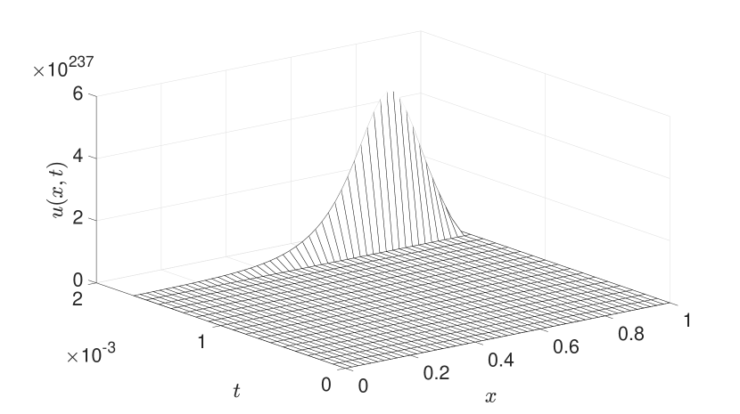
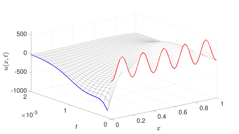
Figure 1: Open-loop response (top) of system (19). Closed-loop response (bottom) of system (19).

IV Conclusion

We proposed in this work the first generalization of Sontag’s formula to systems that admit a CLF whose derivative is not affine in the control input, but polynomial. Depending on the structure of the resulting polynomial, we designed continuous universal controllers that vanish at the origin and achieve stabilization. We proved our results in the context of boundary control of convection-reaction-diffusion PDEs. Finally, our results have been illustrated on a numerical example where the PDE to control possesses a superlinear reaction term that yields finite-time blow-up phenomena. In future work, we would like to guarantee in addition to continuity boundedness of the boundary control input in the context of CRD PDEs. We would also like to see if it is possible to design universal controllers for other structures of the derivative of the CLF, and for more general convective terms, such as a combination of flow convection and counter-convection. It would be also interesting to generalize our approach to higher-order PDEs, such as the Kuramoto-Sivashinsky and the Korteweg-de Vries equations.

References

- [1] Z. Artstein, “Stabilization with Relaxed Controls,” Nonlinear Analysis: Theory, Methods & Applications, vol. 7, no. 11, pp. 1163–1173, 1983.
- [2] E. D. Sontag, “A ‘Universal’ Construction of Artstein’s Theorem on Nonlinear Stabilization,” Systems & control letters, vol. 13, no. 2, pp. 117–123, 1989.
- [3] M. Krstić and H. Deng, Stabilization of Nonlinear Uncertain Systems. Springer, 1998.
- [4] Y. Lin and E. D. Sontag, “A Universal Formula for Stabilization with Bounded Controls,” Systems & control letters, vol. 16, no. 6, pp. 393–397, 1991.
- [5] M. Krstić and P. V. Kokotovic, “Control Lyapunov functions for Adaptive Nonlinear Stabilization,” Systems & Control Letters, vol. 26, no. 1, pp. 17–23, 1995.
- [6] M. Krstić and Z.-H. Li, “Inverse Optimal Design of Input-To-State Stabilizing Nonlinear Controllers,” IEEE Transactions on Automatic Control, vol. 43, no. 3, pp. 336–350, 1998.
- [7] H. Deng, M. Krstić, and R. J. Williams, “Stabilization of Stochastic Nonlinear Systems Driven by Noise of Unknown Covariance,” IEEE Transactions on Automatic Control, vol. 46, no. 8, pp. 1237–1253, 2001.
- [8] D. Liberzon, E. D. Sontag, and Y. Wang, “Universal Construction of Feedback Laws Achieving ISS and Integral-ISS Disturbance Attenuation,” Systems & Control Letters, vol. 46, no. 2, pp. 111–127, 2002.
- [9] N. Marchand, S. Durand, and J. F. G. Castellanos, “A General Formula for Event-Based Stabilization of Nonlinear Systems,” IEEE Transactions on Automatic Control, vol. 58, no. 5, pp. 1332–1337, 2013.
- [10] M. Krstić, “On Global Stabilization of Burgers’ Equation by Boundary Control,” Systems & Control Letters, vol. 37, no. 3, pp. 123–141, 1999.
- [11] W.-J. Liu and M. Krstić, “Stability Enhancement by Boundary Control in the Kuramoto–Sivashinsky Equation,” Nonlinear Analysis: Theory, Methods & Applications, vol. 43, no. 4, pp. 485–507, 2001.
- [12] M. Maghenem, C. Prieur, and E. Witrant, “Boundary Control of the Kuramoto-Sivashinsky Equation Under Intermittent Data Availability,” in American Control Conference (ACC), pp. 2227–2232, 2022.
- [13] M. C. Belhadjoudja, M. Maghenem, E. Witrant, and C. Prieur, “Adaptive Stabilization of the Kuramoto-Sivashinsky Equation Subject to Intermittent Sensing,” in American Control Conference (ACC), pp. 1608–1613, 2023.
- [14] S. Zekraoui, N. Espitia, and W. Perruquetti, “Lyapunov-Based Nonlinear Boundary Control Design with Predefined Convergence for a Class of 1D Linear Reaction-Diffusion Equations,” European Journal of Control, p. 100845, 2023.
- [15] H. Fujita, “On the Blowing Up of Solutions of the Cauchy Problem for ,” J. Fac. Sci. Univ. Tokyo, vol. 13, pp. 109–124, 1966.
- [16] K. Deng and H. A. Levine, “The Role of Critical Exponents in Blow-Up Theorems: The Sequel,” Journal of Mathematical Analysis and Applications, vol. 243, no. 1, pp. 85–126, 2000.
- [17] E. Fernandez-Cara and E. Zuazua, “Null and Approximate Controllability for Weakly Blowing Up Semilinear Heat Equations,” Annales de l’Institut Henri Poincaré C, Analyse non linéaire, vol. 17, no. 5, pp. 583–616, 2000.
- [18] M. Krstić and R. Vazquez, “Nonlinear Control of PDEs: Are Feedback Linearization and Geometric Methods Applicable?,” IFAC Proceedings Volumes, vol. 40, no. 12, pp. 20–27, 2007.
- [19] R. Vazquez and M. Krstić, “Control of 1-D Parabolic PDEs with Volterra Nonlinearities, part I: Design,” Automatica, vol. 44, no. 11, pp. 2778–2790, 2008.
- [20] R. Vazquez and M. Krstić, “Control of 1D Parabolic PDEs with Volterra Nonlinearities, Part II: Analysis,” Automatica, vol. 44, no. 11, pp. 2791–2803, 2008.
- [21] J. Buckmaster, “Viscous Sheets Advancing Over Dry Beds,” Journal of Fluid Mechanics, vol. 81, no. 4, pp. 735–756, 1977.