The low multipoles in the Pantheon+SH0ES data
Abstract
In previous work we have shown that the dipole in the low redshift supernovae of the Pantheon+SH0ES data does not agree with the one inferred from the velocity of the solar system as obtained from CMB data. We interpreted this as the presence of significant bulk velocities. In this paper we study the monopole, dipole and quadrupole in the Pantheon+SH0ES data. We find that in addition to the dipole also both, the monopole and the quadrupole are detected with high significance. They are of similar amplitudes as the bulk flow. While the monopole is only significant at very low redshift, the quadrupole even increases with redshift.
1 Introduction
Standard cosmology assumes a statistically homogeneous and isotropic distribution of matter and radiation in the Universe. Correspondingly, on sufficiently large scales the geometry of the Universe is assumed to deviate little from homogeneity and isotropy, i.e., from a Friedmann-Lemaître (FL) universe. These assumptions are in good agreement with the small fluctuations observed in the Cosmic Microwave Background (CMB), which is isotropic with fluctuations of order , see [1, 2, 3, 4] for the latest results.
Due to our motion with respect to the surface of last scattering, the CMB also exhibits a dipole with an amplitude of about . This dipole has been discovered in the 1970s [5, 6] and is now measured with exquisite precision [7, 8, 1]. This anisotropy in the CMB also leads to a correlation of adjacent multipoles which have consistently been measured with a significance of about 5 standard deviations [9]. Attributing the entire CMB dipole to our motion, one infers a velocity of the solar system given by
| (1.1) |
where are the ‘right ascension’ (ra) and ‘declination’ (dec) denoting the directions with respect to the baricenter of the solar system (at J2000, i.e. January 1, 2000). A possible intrinsic dipole in the CMB of the same order as the higher multipoles is expected to change this result by about 1%.
Within the standard model of cosmology we expect to see this dipole due to our motion also in the large scale distribution of galaxies [10]. While first results of a radio survey agreed reasonably well with the CMB velocity [11], more recent analyses of catalogs of radio galaxies and quasars have found widely differing results from which significantly larger peculiar velocities have been inferred [12, 13, 14, 15, 16]. The latest results [17] show a discrepancy with the CMB dipole which is considered by the authors as a challenge of the cosmological principle. There are, however also critiques that the analysis of the data might be too simplified and that a more refined analysis would give results that are consistent with standard cosmology [18, 19, 20], see also [21] for an alternative method which gives results in agreement with the CMB dipole albeit with large error bars.
In previous work [22] we determined the dipole inferred from the Pantheon+ compilation of type Ia Supernovae [23]. We found a dipole compatible in amplitude with the CMB dipole, but pointing in a different direction. However, the dipole amplitude in supernova distances is proportional to and hence it rapidly decays with redshift so that for supernovae with no significant dipole can be measured. It is therefore possible that the dipole we have seen in this data actually corresponds to the velocity where is the peculiar velocity of the solar system and is the bulk velocity of a sphere around us with radius Mpc, where is the present value of the Hubble parameter. Interestingly, the bulk velocity inferred in this way is in relatively good agreement with the result of the ‘cosmicflow4’ analysis [24], however our error-bars are significantly larger. In the present paper we test this hypothesis. As we discuss in the next section, if the SN dipole is really due to the peculiar motion of the individual supernovae and not due to a global dipole, we expect to observe also a monopole and a quadrupole (and higher multipoles) of similar amplitude. For this reason, we determine in this paper also the monopole and the quadrupole of the Pantheon+ compilation of supernova distances, in addition to the bulk flow (dipole) – a possible quadrupolar Hubble expansion in Pantheon+ was also studied in [25] with the help of a cosmographic expansion. We do indeed find a monopole and a quadrupole with amplitudes of the expected order of magnitude. We also argue that this amplitude for the bulk velocity is not extremely unlikely in the standard CDM model.
Notation : We consider a spatially flat FL universe with linear scalar perturbations in Newtonian gauge,
| (1.2) |
The two metric perturbations and are the Bardeen potentials. Einstein’s summation convention is assumed. Spatial vectors are denoted in bold face. The derivative with respect to conformal time is indicated as an overdot. is the comoving Hubble parameter, while the physical Hubble parameter is given by . We work in units where the speed of light is unity but, for the convenience of the reader, we present our results on velocities in km/s.
2 Theoretical description
In our previous paper [22], we have found that even after subtracting the observer velocity , assumed to be the one seen in the CMB data, there remains a significant dipole in the supernova distances of the Pantheon+ compilation. We now want to study whether there are also significant monopole and quadrupole contributions. At first order in cosmological perturbation theory, the luminosity distance out to a source at observed redshift in direction is, up to some small local contributions which we neglect here, given by [26, 27, 28]:
| (2.1) | |||||
Here is the observer velocity, is the comoving distance out to redshift , is the peculiar velocity of the source. The functions are to be evaluated at and . The symbol denotes the Laplacian on the sphere, while is the luminosity distance of the background FL universe. In a flat CDM universe at low redshift where radiation can be neglected it is given by
| (2.2) |
2.1 The monopole and quadrupole perturbations of the luminosity distance at low redshift
In what follows we only retain the terms in the perturbation of the luminosity distance. These terms dominate the fluctuations at small redshift. For we may approximate by
| (2.3) |
For small redshifts, this term dominates over the other contributions since it is enhanced by a factor and since, at low redshift, velocities are about two orders of magnitude larger than the Bardeen potentials. Using that et we can write (2.3) as
| (2.4) |
If the source peculiar velocity were independent of direction, a pure ‘bulk velocity’ shared by all supernovae, this would lead to a pure dipole, which is what we considered in our previous paper. However, we expect that there should also be some dependence on direction and on redshift. Here we assume that the redshift dependence is the one given by linear perturbation theory, this is a reasonable assumption for the large scales that we investigate (e.g. corresponds to a radius of Mpc). We then fit for an angular dependence in the form of a monopole and a quadrupole. Of course we expect in principle also higher multipoles to be present but we neglect them here. As the different multipoles are orthogonal to each other, this should not bias our results on the monopole, dipole and quadrupole. Within linear perturbation theory, the time dependence of the peculiar velocity field is given by
where is the linear growth function and the overdot denotes a derivative with respect to conformal time. Introducing the growth rate defined as [29]
| (2.5) |
we can write
With this, (2.4) becomes
| (2.6) |
As mentioned above, if is independent of direction we obtain simply a dipole. Here we now go one step further by allowing for a dipole, a monopole and a quadrupole in the directional dependence,
| (2.7) |
In this expression, is a symmetric traceless tensor which represents the ‘bulk quadrupole’ today, and since , corresponds to a monopole, the part of that is parallel to the radial direction . Both, and have the units of a velocity. Putting all of this together we obtain
| (2.8) |
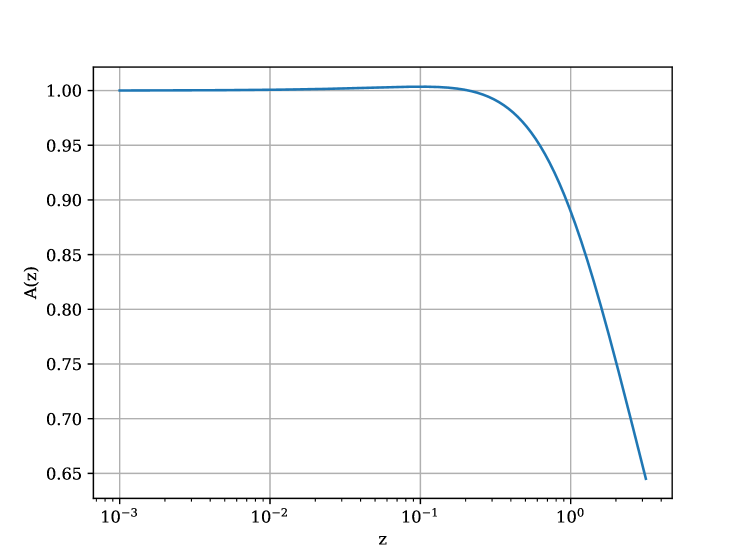
where we defined the prefactor as
| (2.9) |
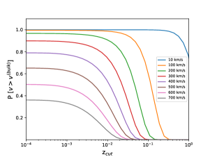
The trace can be distinguished from via its redshift dependence which differs from . A short inspection shows that the ratio between these redshift dependencies, , is well approximated by and therefore becomes large at very low redshifts.
In Fig. 1 we show the behaviour of the prefactor . At small redshifts, , we find that , implying that the correction due to this factor is negligible, in agreement with the assumption of a bulk motion of nearby galaxies.
In our assumption of a flat CDM universe, it is possible to obtain an analytical expression for the linear growth function and the growth rate:
| (2.10) |
| (2.11) |
with
| (2.12) |
2.2 Redshift corrections
The velocity-dependent terms in actually stem from the fact that peculiar velocities modify the observed redshifts. They are the first terms in a Taylor series in . It might be more accurate to directly correct the redshift by subtracting inside the expression for . This is the method used in [23] and we also adopt it here. The redshift correction due to the motion of the solar system is given by
| (2.14) |
where
| (2.15) |
with .
Similarly, we consider the redshift correction due to the peculiar motion of the supernovae relative to the solar system which we model as a bulk velocity, a monopole and a quadrupole,
| (2.16) |
where, similar to (2.15), is given by
| (2.17) |
with given by
| (2.18) |
We can then rewrite (2.8) more concisely as
| (2.19) |
3 Data and methodology
As in our previous work [22], we use the Pantheon+ data which provides distance moduli for 1550 SNe,
| (3.1) |
As reported in Tab. 8, 77 SNe are in galaxies that also host Cepheids, for which we know the absolute distance modulus . While Pantheon+ uses corrected redshifts including the motion of the solar system and estimated peculiar velocities of the sources, we use the actually measured redshifts for our analysis.
For handling the astronomical quantities and convenient unit conversions we use the package astropy [32, 33, 34]. To determine the parameters of our model we perform an MCMC analysis using the python package emcee [35]. Our code is parallelized using the Python package schwimmbad [36]. Our sampler consists of 32 walkers with the “stretch move” ensemble method described in [37].
As in our previous paper, we maximize the likelihood
| (3.2) |
where is the covariance matrix provided by the Pantheon+ collaboration. The vector is defined by
| (3.3) |
where
| (3.4) |
and is given in (2.19). In Eq. (3.3) we introduce the nuisance parameter dM which is constrained by the supernovae in Cepheid-host galaxies, while the supernovae in galaxies not hosting Cepheids constrain the luminosity distance parameters.
Finally, we analyse our chains using the getdist package [38]. Following the emcee guidelines (the interested reader is referred to https://emcee.readthedocs.io/en/stable/tutorials/autocorr/), we use the integrated [37] as convergence diagnostics. Here can be considered as the number of steps necessary for the chain to forget where it started. In particular, we assume that the chain is converged with respect to a certain parameter when the number of steps in the chain is larger than 50 times the auto-correlation time, . We further consider as burn-in and discard the first steps, where is the maximum value for all the parameters. In all MCMC analyses, we use uniform priors as reported in Table 1 for the parameters that are varied.
| Parameter | Prior range |
|---|---|
| [0, 1000] km/s | |
| ra | [0°, 360°] |
| [-1, 1] | |
| [-500,500] km/s | |
| [-500,500] km/s | |
| dM | [-0.5, 0.5] |
| [40, 100] km/s/Mpc | |
| [0, 1] |
4 Results
As first step, in order to test our code and the theoretical assumptions, we perform a similar analysis for the dipole only as in our previous paper [22], but applying the redshift correction as described in Section 2.2, neglecting peculiar velocity corrections.
As we see in Figure 2, we obtain the same contours as in our previous paper where the corrections were applied at the level of the definition of luminosity distance instead of the redshift, i.e., using only the first term in the Taylor series in and linearizing in (neglecting bulk velocity, the monopole and the quadrupole). The robustness of applying redshift corrections is also manifest by the fact that, when considering the dipole only, we find a negligible difference of with respect to the analysis developed in the previous paper where we used Eq. (2.11). In Table 2 we report the constraints inferred from the MCMC routine for the new orange contours, where the bulk velocity correction is taken into account as a redshift correction. Note that while the amplitude roughly agrees with the velocity of the solar system inferred from the CMB, the direction is very different, compared with Eq. (1.1). This result is in excellent agreement with our previous paper [22], where it was the main finding. It led us to the conclusion that the bulk velocity cannot be neglected.
| [km/s] | ra[°] | dec[°] | dM | [km/s/Mpc] | |
|---|---|---|---|---|---|
4.1 Bulk velocity
When fixing to the Planck value and including just the correction in Equation (2.17), i.e. considering only the first term in brackets in Equation (2.18), the dipole, we obtain the contour plots shown in Figure 3 and reported in Table 3. These bulk velocities agree with our previous paper [22].
4.2 Bulk + quadrupole analysis
We now include also the quadrupole in the luminosity distance, which actually comes from the dipole in the peculiar velocity and which we describe by the matrix , to perform a bulk + quadrupole analysis. As mentioned in Section 2.1, is a symmetric trace-less tensor of dimension . It is defined by five parameters that we introduce in our MCMC routine.
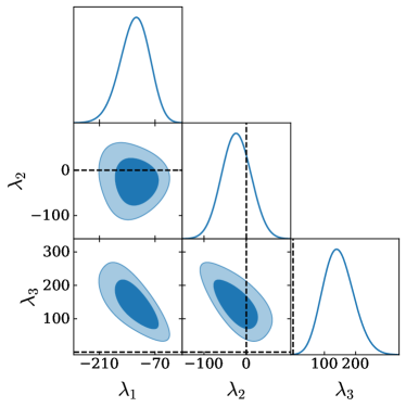
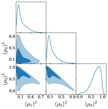
Using the samples obtained for the matrix elements , we determine the contour plots for the eigenvalues which are shown in Figure 4 and reported in Table 4.
| [km/s] | [km/s] | [km/s] |
|---|---|---|
In our parametrisation of the matrix the trace vanishes, hence the sum of the eigenvalues is zero by construction. However, eigenvalues and differ from zero by 3 to 4 standard deviations. Since their distributions are close to Gaussian, see Fig. 4, we conclude that the detection of the quadrupole is significant. The direction of the eigenvectors is fixed up to a sign. To remove this ambiguity, we choose all eigenvectors to point into the northern hemisphere. They are normalized and dimensionless, since we assume the eigenvalues to have the dimension of velocity. In Table 5 we report their directions. As is compatible with zero, it is not surprising that the direction of is not well determined. However, also the direction of has surprisingly large errors.
To compare the amplitude of the quadrupole with the bulk flow, we define
| (4.1) |
and compare it with obtained in the bulk + quadrupole analysis. While km/s, we find km/s.111Errors associated to are computed using the python package uncertainties [39]. Even though the quadrupole is somewhat smaller than the dipole, it is of a comparable order of magnitude.
| ra [°] | dec [°] | [(km/s)2] | |
|---|---|---|---|
In Fig. 5 and Table 5 we also show the scalar products . Note that the sign has no significance since both and are eigenvectors of . Since the direction of is not well determined the value of is also not. Interestingly, is well aligned with and, as a consequence, is nearly orthogonal to .
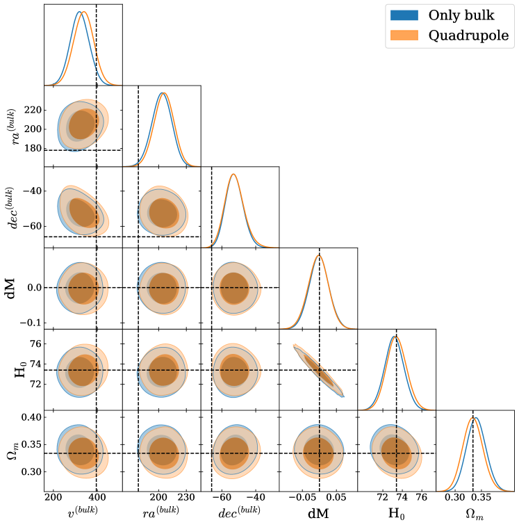
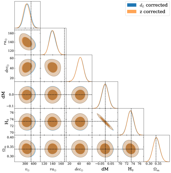
In Fig. 6 we compare the inferred cosmological parameters and the bulk velocity in an analysis including the quadrupole from the bulk motion (orange) with the one including only the dipole. We find that all values are virtually identical in both analyses. It is not surprising that the dipole is not changed, as we expect different multipoles to be independent, but we note that also the cosmological parameter constraints stay the same.
4.3 Bulk + monopole analysis
We also model the data by adding a monopole to the bulk velocity, the parameter of Eq. (2.18). Interestingly, while adding a quadrupole with its five free parameters reduces the by the modest value with respect to the analysis including only a bulk velocity, by adding a monopole characterized by just one free parameter, , we gain a . The inclusion of the monopole also leads to a slight increase of , by and to a decrease of by about , see Table 6. The increase of can be understood as follows: a negative value of leads to an increase in hence the measured . And since is inversely proportional to , this implies a larger . At this reduction of is about 1.2%, but due to the reduced value of , it decays rapidly and is only about 0.02% at . The difference crosses zero at , above which the Pantheon+ dataset contains no SNIa.
However, like the quadrupole the monopole does not affect the dipole, . This again is a consequence of the fact that the different multipoles are orthogonal functions. As the background luminosity distance is a monopole, only the monopole of the peculiar velocity, i.e. its radial component, can affect the it and thereby modify the inferred cosmological parameters.
| [km/s] | [km/s] | ra(bulk)[°] | dec(bulk)[°] | [km/s/Mpc] | |
|---|---|---|---|---|---|
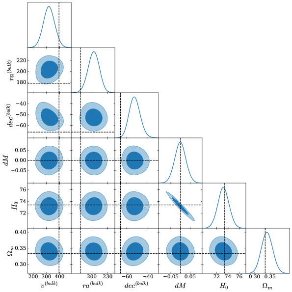
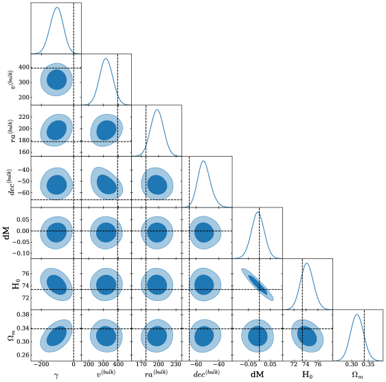
The contour plots for this analysis are shown in Fig. 7. Note the correlation between and and the anti-correlation of and . Despite the relatively low best fit amplitude of the monopole, about of the bulk velocity, its impact on the cosmological parameters is quite strong. Note also that the monopole is distinguished from the background luminosity distance only via its redshift dependence. Nevertheless, it is detected with a significance of more than . As we shall see, this is mainly due to its strong effect at very low redshift.
4.4 The full bulk + quadrupole + monopole analysis
Finally we model the redshift by adding all, the radial velocity (monopole), the bulk velocity (dipole) and the quadrupole. With respect to the analysis allowing only for a bulk velocity (dipole), we gain a in this model which has six additional parameters. As we have seen in the previous section, most of this improvement is due to the monopole. The contour plots of this analysis are shown in Fig. 8 and the best fit values with error bars are reported in Table 7. As already in the pure monopole analysis, the monopole amplitude, is correlated with and . The best fit values of and are affected by the presence of , but the values found in the original Pantheon+ analysis [23] remain consistent within with our results.
| zcut | ra(bulk) | dec(bulk) | |||||||
|---|---|---|---|---|---|---|---|---|---|
| [km/s] | [km/s] | [deg] | [deg] | [km/s/Mpc] | [km/s] | [km/s] | [km/s] | ||
| No cut | |||||||||
| 0.005 | |||||||||
| 0.01 | |||||||||
| 0.0175 | |||||||||
| 0.025 | |||||||||
| 0.0375 | |||||||||
| 0.05 |
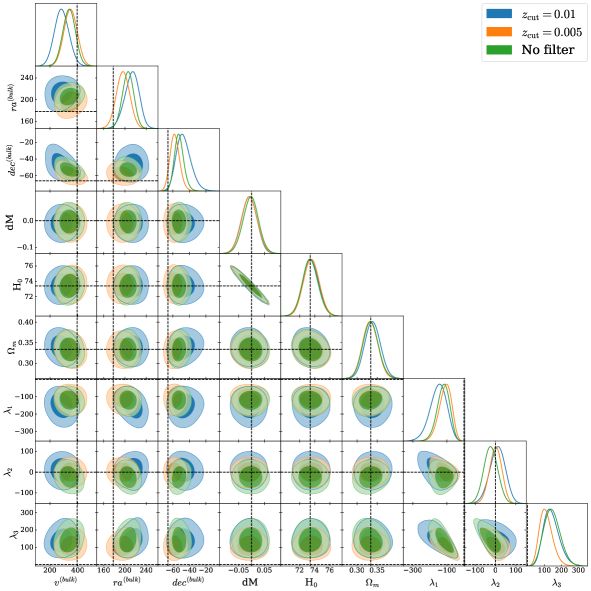
4.5 Applying redshift cuts
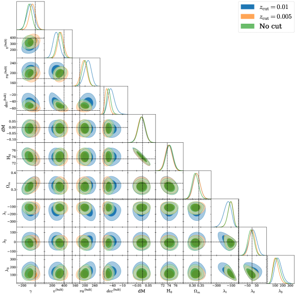
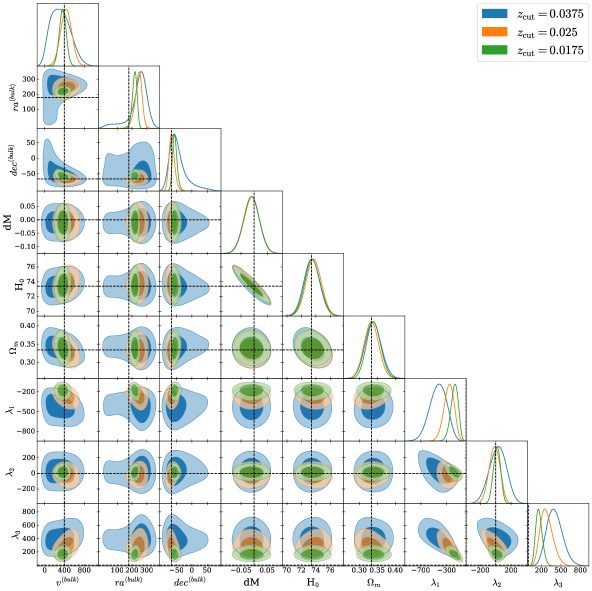
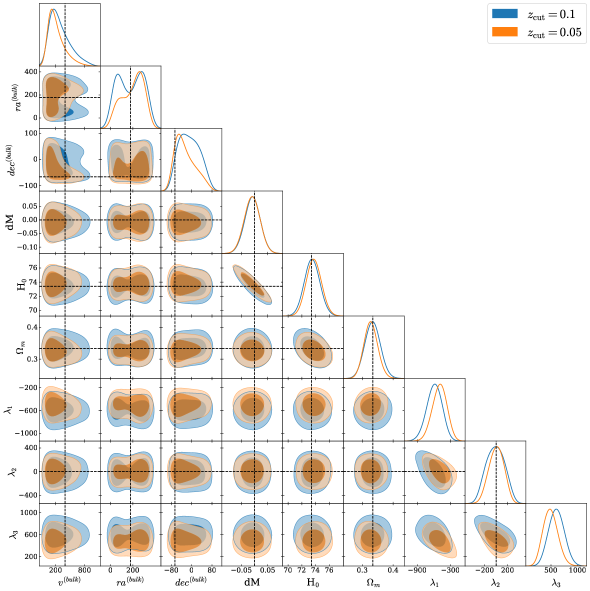
We repeat our bulk + monopole + quadrupole analysis to sub-portion of the Pantheon+ dataset obtained removing all the supernovae with a redshift smaller than a certain values . We obtain the contour plots reported in Figs. 8, 9 and in Appendix A, Figs. 13 and 14. In Table 8 we report the number of supernovae included within a given redshift cut.
| zcut | Pantheon+ | SNe in | |
|---|---|---|---|
| without Cepheids | Cepheid hosts | ||
| No cut | 1624 | 77 | |
| 0.005 | 1615 | 50 | |
| 0.01 | 1576 | 7 | |
| 0.0175 | 1468 | 2 | |
| 0.025 | 1312 | 0 | |
| 0.0375 | 1126 | 0 | |
| 0.05 | 1054 | 0 | |
| 0.1 | 960 | 0 |
| ra(bulk) | dec(bulk) | |||||||
|---|---|---|---|---|---|---|---|---|
| [km/s] | [deg] | [deg] | [km/s/Mpc] | [km/s] | [km/s] | [km/s] | ||
| No cut | ||||||||
| 0.005 | ||||||||
| 0.01 | ||||||||
| 0.0175 | ||||||||
| 0.025 | ||||||||
| 0.0375 | ||||||||
| 0.05 | ||||||||
| 0.1 |
Our results are also summarized in tables 7, where the full analysis is presented and in table 9 where we do not include the monopole. Note that already at , the monopole is no longer detected at more than . It is significant only at very low redshifts where it is multiplied by a factor Nevertheless, its presence does somewhat raise the inferred value of the Hubble parameter, albeit within and not in the direction which would reduce the Hubble tension. Note also that for the first redshift cut only 9 Supernovae in galaxies without Cepheids and 27 supernovae in galaxies with Cepheids are removed, see table 8. Hence most of the monopole signal comes from modelling these 9 lowest redshift supernovae.
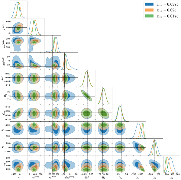
In table 7 we do not include the redshift cut since for this cut the likelihood contours become very flat and good convergence cannot be reached. For this reason we also include the redshift-cut study without the monopole reported in table 9. This MCMC converges well also for . The results for the bulk velocity and the quadrupole of this analysis are in good agreement with the full analysis. It is interesting to note that while for the dipole, i.e., the bulk velocity, is no longer detected and more than , see table 9 and Figs. 13 and 14, the eigenvalues and of the quadrupole remain non-zero even at 95% confidence. Contrary to the bulk velocities, the eigenvalues and of the quadrupole are even increasing with redshift cut. This means that above , corresponding to a distance Mpc, the angular fluctuations in the luminosity distance are better fitted with a quadrupole than with a dipole. This is not so surprising as the quadrupole represents fluctuating velocity field roughly on the scale of the redshift cut while the bulk velocity is assumed to be constant on all scales relevant in the analysis.
4.6 analysis
It is also interesting to study the improvement of the fit when including the monopole and quadrupole. As shown in Table 10, this strongly depends on the redshift cut. Introducing no cut the fit is significantly improved and as we have seen this is mainly due to the monopole. At the very low cuts of and corresponding to a radius of Mpc and Mpc, the improvement is not significant considering that we have introduced 5 or, with monopole 6, additional parameters. However, for , is monotonically increasing and for , the improvement obtained by including a quadrupole (and a at this redshift irrelevant monopole) is, even if not overwhelming, more substantial. This is due to the fact that even for the highest redshift cuts, and are non-zero within 95% confidence. In the contrary, their best fit values are even increasing. Even though also the error bars increase, the significance of and simply measured as (best fit value)/error also increases with redshift. This is not the case for which can vanish within less than 90% confidence for and becomes even less significant with increasing redshift, see Table 9 and Figs. 13 and 14 in Appendix A.
| Bulk + quadrupole | Bulk + quadrupole | |
| + monopole | ||
| No cut | ||
| - | ||
4.7 Mock tests
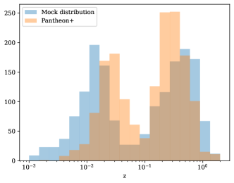
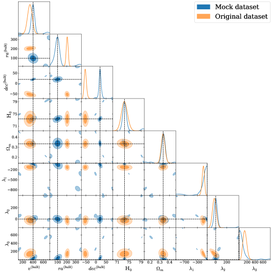
In order to confirm the significance of the monopole, quadrupole and the bulk velocity, we have also compared the analysis of the true Pantheon+ data with the analysis of a mock dataset created using an artificial redshift distribution (the comparison with the original redshift distribution is in Fig. 10), the distance moduli computed according to Eqs. (2.16, 2.18, 2.19), fixing a constant km/s in direction °, °), so that the monopole and quadrupole vanish, and a cosmology given by the fiducial values , . Moreover, for simplicity, we neglected supernovae hosted in cepheids and fixed dM=0, and we used a diagonal covariance whose elements are the same as the diagonal of the covariance matrix of the Pantheon+ analysis.
For , and the bulk velocity we are able to recover the values chosen for the construction of the mock dataset. At the same time, we do not find any monopole or quadrupole as they are detected in the real data. In Fig. 11 we show the results from a parameter estimation of the Mock dataset compared to the real data for dipole and quadrupole only. The bulk velocity inserted in the Mock data and the cosmological parameters used are indicated by dashed vertical and horizontal lines. Clearly, the input parameters are very well reproduced and all three eigenvalues of the quadrupole peak at zero. The same is true for the monopole. This confirms our interpretation that the bulk velocity, the monopole and the quadrupole are present in the data.
5 Conclusions
In this paper we analysed the Pantheon+ data including a dipole, a quadrupole and a monopole perturbation in the luminosity distance which are motivated by the peculiar motion of the supernovae which leads to an angular dependence of the redshift perturbation. We have found that both, the quadrupole and at very low redshift also the monopole are significant and roughly of the same amplitude as the dipole of the bulk velocity. Removing low redshift supernovae from our sample, we even find that while the monopole and the dipole from the bulk motion are no longer detected with high significance, the quadrupole remains non-zero at more than 95% confidence. It is also interesting to note that the eigenvalues of the quadrupole are even significantly increasing with redshift while their errors stay roughly constant. Hence they also become more significant at higher redshift. This trend is understandable as at higher redshifts, where neither the monopole perturbation nor the dipole (bulk velocity) are significant, the peculiar velocity of the sources has to be modelled by the quadrupole alone in our approach.
It is intriguing that our result for the bulk velocity is within 95% confidence in agreement with the bulk flow found in the CosmicFlows4 analysis [24]. That it does not perfectly agree with CosmicFlows4 is not surprising since our means that we exclude all supernovae inside a ball of radius . While the remaining bulk flow is dominated by the one in a shell close to , this is not quite the same as the velocity inside the ball. Also, while the CosmicFlows4 analysis does include the Pantheon+ data, it has a much larger catalog of about 38’000 galaxy velocities. For we obtain a bulk flow of about km/s, and based on Appendix B, see also Fig. 12, we find the probability to find a velocity of this size or larger inside a ball of redshift is
| (5.1) |
This is the result within standard CDM with Mpckm/s. This seems to be in tension with the standard model at nearly two . However, taking into account that our error in is relatively large we also have to consider km/s, for which we find
| (5.2) |
for which certainly there is no tension. The reason that our results are not in strong tension with CDM is mainly due to the weaker statistical power, hence to the large error bars of and to the fact that we have no truly significant bulk flow at Mpc. Would we take at face value the bulk flow of 280km/s at which corresponds to Mpc, with Mpckm/s, we would find
| (5.3) |
This would be similar to the findings of Ref. [24]. But since this bulk velocity is compatible at 68% confidence, see Fig. 14, with the nominally expected value of km/s, this is certainly not a valid conclusion.
Within the statistical power of the Pantheon+ data, we therefore conclude that the inferred mmonopole perturbation, dipole and quadrupole in the Pantheon+ data are in reasonable agreement with a velocity field expected in the standard CDM model of cosmology. It will certainly be very important to repeat this analysis with a larger sample of supernovae. Especially low redshift supernovae with are suited to improve the statistical power. For example, the Vera Rubin Observatory’s LSST should be able to detect up to supernovae within a year or so in this redshift range [40], while the Pantheon+ dataset has 800 sources in this redshift range.
Acknowledgments
The authors acknowledge financial support from the Swiss National Science Foundation. The computations were performed at University of Geneva using Baobab HPC service.
Appendix A Pantheon+ redshift dependence
In this appendix we also show the contour plots for higher redshift cuts for both the bulk + quadrupole analysis and the full bulk + quadrupole + monopole analysis. We choose and in Fig. (13, 15) for both the analyses, whereas we set and in Figs. 14, for only the bulk + quadrupole analysis.
Appendix B Statistical properties of the velocity field
In the standard cosmological model, the velocity field is the gradient of a scalar velocity potential , . The velocity potential is an isotropic Gaussian random field with zero mean and power spectrum (at ) . This implies that each component of the velocity field is itself an isotropic Gaussian random field, and in Fourier space is given by
| (B.1) |
The variance of the fields and are then related through
| (B.2) |
Thanks to the statistical isotropy of the velocity field, each component contributes equally to , so that the prefactor is on average, and
| (B.3) |
Here we are interested in the variance of the velocity field when averaged over a spatial volume of a given size ,
| (B.4) |
for a given window function that describes the shape of the spatial volume. For a spherical top-hat window in real space, the Fourier-space window function is
| (B.5) |
In perturbation theory, the power spectrum of is related to the power spectrum of the density contrast through
| (B.6) |
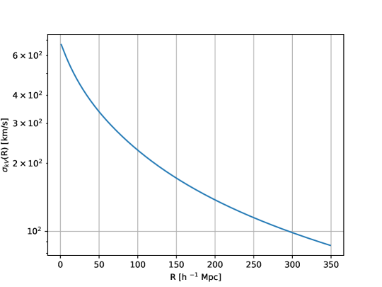
where is the growth factor today in the CDM model. We show as a function of in Fig. 16.222For computing the power spectrum used in the probability analysis we used the boltzmann solver camb [41], assuming =73.4 km/s/Mpc and =0.338 for the background cosmology.
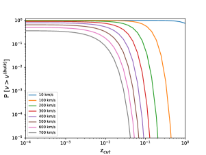
In order to evaluate the probability for finding a larger bulk velocity on a given scale than a certain value we consider the random variable
| (B.7) |
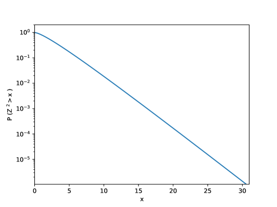
which has zero mean and unit variance. Its norm-squared, then has a distribution with 3 degrees of freedom (and has a distribution). The probability to find a value larger than for a random variable that has a distribution with degrees of freedom is
| (B.8) |
where is the incomplete Gamma function. We show this probability for in Fig. 17. From Fig. 16 we see that on a scale of Mpc which corresponds to , we find km/s. In our analysis we find a mean value of km/s inside this redshift cut. For a distribution, we obtain
| (B.9) |
While this probability is not very high, it is by no means excluding the model.
References
- [1] Planck Collaboration, N. Aghanim et al., Planck 2018 results. I. Overview and the cosmological legacy of Planck, Astron. Astrophys. 641 (2020) A1, [arXiv:1807.06205].
- [2] Planck Collaboration, N. Aghanim et al., Planck 2018 results. VI. Cosmological parameters, Astron. Astrophys. 641 (2020) A6, [arXiv:1807.06209]. [Erratum: Astron.Astrophys. 652, C4 (2021)].
- [3] ACT Collaboration, S. Aiola et al., The Atacama Cosmology Telescope: DR4 Maps and Cosmological Parameters, JCAP 12 (2020) 047, [arXiv:2007.07288].
- [4] SPT-3G Collaboration, L. Balkenhol et al., Measurement of the CMB temperature power spectrum and constraints on cosmology from the SPT-3G 2018 TT, TE, and EE dataset, Phys. Rev. D 108 (2023), no. 2 023510, [arXiv:2212.05642].
- [5] E. K. Conklin, Velocity of the Earth with Respect to the Cosmic Background Radiation, Nature 222 (June, 1969) 971–972.
- [6] P. S. Henry, Isotropy of the 3 K Background, Nature 231 (June, 1971) 516–518.
- [7] A. Kogut et al., Dipole anisotropy in the COBE DMR first year sky maps, Astrophys. J. 419 (1993) 1, [astro-ph/9312056].
- [8] Planck Collaboration, N. Aghanim et al., Planck 2013 results. XXVII. Doppler boosting of the CMB: Eppur si muove, Astron. Astrophys. 571 (2014) A27, [arXiv:1303.5087].
- [9] S. Saha, S. Shaikh, S. Mukherjee, T. Souradeep, and B. D. Wandelt, Bayesian estimation of our local motion from the Planck-2018 CMB temperature map, JCAP 10 (2021) 072, [arXiv:2106.07666].
- [10] G. F. R. Ellis and J. E. Baldwin, On the expected anisotropy of radio source counts, MNRAS 206 (Jan., 1984) 377–381.
- [11] C. Blake and J. Wall, Quantifying angular clustering in wide-area radio surveys, Mon. Not. Roy. Astron. Soc. 337 (2002) 993, [astro-ph/0208350].
- [12] P. Tiwari and A. Nusser, Revisiting the NVSS number count dipole, Journal of Cosmology and Astroparticle Physics 2016 (mar, 2016) 062–062.
- [13] C. A. P. Bengaly, R. Maartens, and M. G. Santos, Probing the Cosmological Principle in the counts of radio galaxies at different frequencies, JCAP 04 (2018) 031, [arXiv:1710.08804].
- [14] J. Colin, R. Mohayaee, M. Rameez, and S. Sarkar, Evidence for anisotropy of cosmic acceleration, Astron. Astrophys. 631 (2019) L13, [arXiv:1808.04597].
- [15] N. J. Secrest, S. v. Hausegger, M. Rameez, R. Mohayaee, S. Sarkar, and J. Colin, A test of the cosmological principle with quasars, The Astrophysical Journal 908 (2021), no. 2 L51, [arXiv:2009.14826].
- [16] Siewert, Thilo M., Schmidt-Rubart, Matthias, and Schwarz, Dominik J., Cosmic radio dipole: Estimators and frequency dependence, A&A 653 (2021) A9.
- [17] N. J. Secrest, S. von Hausegger, M. Rameez, R. Mohayaee, and S. Sarkar, A Challenge to the Standard Cosmological Model, Astrophys. J. Lett. 937 (2022), no. 2 L31, [arXiv:2206.05624].
- [18] C. Dalang and C. Bonvin, On the kinematic cosmic dipole tension, Mon. Not. Roy. Astron. Soc. 512 (2022), no. 3 3895–3905, [arXiv:2111.03616].
- [19] C. Guandalin, J. Piat, C. Clarkson, and R. Maartens, Theoretical systematics in testing the Cosmological Principle with the kinematic quasar dipole, arXiv:2212.04925.
- [20] Y.-T. Cheng, T.-C. Chang, and A. Lidz, Is the Radio Source Dipole from NVSS Consistent with the CMB and CDM?, arXiv:2309.02490.
- [21] P. da Silveira Ferreira and V. Marra, Tomographic redshift dipole: Testing the cosmological principle, arXiv:2403.14580.
- [22] F. Sorrenti, R. Durrer, and M. Kunz, The dipole of the pantheon+sh0es data, Journal of Cosmology and Astroparticle Physics 2023 (nov, 2023) 054.
- [23] D. Brout et al., The Pantheon+ Analysis: Cosmological Constraints, Astrophys. J. 938 (2022), no. 2 110, [arXiv:2202.04077].
- [24] R. Watkins, T. Allen, C. J. Bradford, J. Ramon, Albert, A. Walker, H. A. Feldman, R. Cionitti, Y. Al-Shorman, E. Kourkchi, and R. B. Tully, Analysing the large-scale bulk flow using cosmicflows4: increasing tension with the standard cosmological model, Monthly Notices of the Royal Astronomical Society 524 (07, 2023) 1885–1892, [https://academic.oup.com/mnras/article-pdf/524/2/1885/50877754/stad1984.pdf].
- [25] J. A. Cowell, S. Dhawan, and H. J. Macpherson, Potential signature of a quadrupolar hubble expansion in Pantheon+supernovae, Monthly Notices of the Royal Astronomical Society 526 (09, 2023) 1482–1494, [https://academic.oup.com/mnras/article-pdf/526/1/1482/51791200/stad2788.pdf].
- [26] C. Bonvin, R. Durrer, and M. A. Gasparini, Fluctuations of the luminosity distance, Phys. Rev. D 73 (2006) 023523, [astro-ph/0511183]. [Erratum: Phys.Rev.D 85, 029901 (2012)].
- [27] L. Hui and P. B. Greene, Correlated fluctuations in luminosity distance and the importance of peculiar motion in supernova surveys, Physical Review D 73 (jun, 2006).
- [28] S. G. Biern and J. Yoo, Gauge-Invariance and Infrared Divergences in the Luminosity Distance, JCAP 04 (2017) 045, [arXiv:1606.01910].
- [29] R. Durrer, The Cosmic Microwave Background. Cambridge University Press, 12, 2020.
- [30] E. V. Linder and R. N. Cahn, Parameterized beyond-einstein growth, Astroparticle Physics 28 (dec, 2007) 481–488.
- [31] Euclid Collaboration, G. Jelic-Cizmek et al., Euclid Preparation. TBD. Impact of magnification on spectroscopic galaxy clustering, arXiv:2311.03168.
- [32] Astropy Collaboration and Astropy Project Contributors, Astropy: A community Python package for astronomy, Astron. Astrophys. 558 (Oct., 2013) A33, [arXiv:1307.6212].
- [33] Astropy Collaboration and Astropy Project Contributors, The Astropy Project: Building an Open-science Project and Status of the v2.0 Core Package, Astron. J. 156 (Sept., 2018) 123, [arXiv:1801.02634].
- [34] Astropy Collaboration and Astropy Project Contributors, The Astropy Project: Sustaining and Growing a Community-oriented Open-source Project and the Latest Major Release (v5.0) of the Core Package, Astrophys. J. 935 (Aug., 2022) 167, [arXiv:2206.14220].
- [35] D. Foreman-Mackey, D. W. Hogg, D. Lang, and J. Goodman, emcee: The MCMC Hammer, Publ. Astron. Soc. Pac. 125 (Mar., 2013) 306, [arXiv:1202.3665].
- [36] A. M. Price-Whelan and D. Foreman-Mackey, schwimmbad: A uniform interface to parallel processing pools in python, The Journal of Open Source Software 2 (sep, 2017).
- [37] J. Goodman and J. Weare, Ensemble samplers with affine invariance, Communications in Applied Mathematics and Computational Science 5 (Jan., 2010) 65–80.
- [38] A. Lewis, Getdist: a python package for analysing monte carlo samples, 2019.
- [39] E. O. LEBIGOT, “Uncertainties: a python package for calculations with uncertainties.” http://pythonhosted.org/uncertainties/.
- [40] LSST Dark Energy Science Collaboration, V. Petrecca, M. T. Botticella, E. Cappellaro, L. Greggio, B. Sánchez, A. Möller, M. Sako, M. Graham, M. Paolillo, and F. Bianco, Recovered SN Ia rate from simulated LSST images, arXiv:2402.17612.
- [41] A. Lewis, “CAMB Notes.” https://cosmologist.info/notes/CAMB.pdf.