All-in-One: Heterogeneous Interaction Modeling for Cold-Start Rating Prediction

Abstract

Cold-start rating prediction is a fundamental problem in recommender systems that has been extensively studied. Many methods have been proposed that exploit explicit relations among existing data, such as collaborative filtering, social recommendations and heterogeneous information network, to alleviate the data insufficiency issue for cold-start users and items. However, the explicit relations constructed based on data between different roles may be unreliable and irrelevant, which limits the performance ceiling of the specific recommendation task. Motivated by this, in this paper, we propose a flexible framework dubbed heterogeneous interaction rating network (HIRE). HIRE dose not solely rely on the pre-defined interaction pattern or the manually constructed heterogeneous information network. Instead, we devise a Heterogeneous Interaction Module (HIM) to jointly model the heterogeneous interactions and directly infer the important interactions via the observed data. In the experiments, we evaluate our model under three cold-start settings on three real-world datasets. The experimental results show that HIRE outperforms other baselines by a large margin. Furthermore, we visualize the inferred interactions of HIRE to confirm the contribution of our model.

I Introduction

Rating prediction is a crucial task in recommender systems for estimating a user’s preference score on an item, which has wide-ranging applications [1, 2, 3, 4, 5] in e-commerce, online education, and entertainment platforms. In cold-start scenarios, where new users/items have limited information for prediction, accurate rating prediction is essential to attract and retain users (in the case of cold-users) and promote and market items (in the case of cold-items). Due to scarce ratings and interactions, prediction in cold-start scenarios presents a significant challenge, since current recommendation models heavily rely on the observed ratings and interactions to make predictions. To improve prediction accuracy, current solutions introduce explicit additional associations and side information to enrich the features of cold users and items. These approaches can be generally categorized into three lines of research.

As the most traditional approach, collaborative filtering (CF) [6, 7, 8, 9, 10, 11, 12] assumes similar users and items share similar ratings and exploits the user-item interactions to make the rating prediction. Recently, classical CF models have been empowered by neural networks to better incorporate the side information such as user profiles and item descriptions to encode user embeddings [8]. However, CF models can only model a single type of interactions and fail to generalize well to cold users/items with scarce rating interactions.

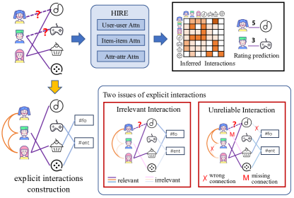
Figure 1: An illustrative example: two main obstacles of existing approaches by exploiting interactions. To predict the first girl’s preference for music, relation between the girl and a boy seems to be irrelevant. The wrong label food for music is also unreliable for rating prediction. HIRE directly models heterogeneous interactions in a data-driven way.

To address the issue of extreme cold users/items, social recommendation approaches [13, 14, 15, 16, 17, 18, 19] extend the scope of interactions and introduce social connections to aid the recommendation task. The intuition behind this approach is that users’ preferences are highly influenced by their social communities and opinion leaders in social networks. Social relationships, collected from multiple sources, can be utilized to enhance modeling of user-item interactions, thereby alleviating the cold-start problem to some extent. However, the effectiveness of such approaches is limited by the usability and reliability of social relations. Firstly, abundant social relations are not always available due to privacy issues and data integration. For example, in some e-commerce scenarios, there are no explicit social relations between customers. Secondly, for specific recommendation tasks, irrelevant social relations can introduce noise and lead to inaccurate predictions. For instance, teenagers are more likely to rate action movies highly based on their friends’ opinions rather than their teachers’, indicating that the interaction between teachers and teenagers is irrelevant when it comes to rate action movies.

Furthermore, recent research has started to involve more complex interactions by constructing heterogeneous information networks (HINs) on entities other than users and items, such as tags and points of interest (POIs). HINs are expected to include richer semantic information and further enhance the quality of representations of users and items. Graph Neural Networks [20] and meta-path embedding [21] are two commonly-used approaches to extract users’ and items’ embeddings from HINs, enabling rating predictions based on such embeddings. However, HIN-based approaches rely on pre-defined graph structures and are therefore vulnerable to the noise and mistakes introduced during the graph construction process. They also suffer from the issue of irrelevance, similar to social recommendation approaches.

To summarize, the homogeneity, unreliability and irrelevancy introduced by the explicit interactions present significant obstacles for existing recommendation approaches, especially for the cold-start scenarios. Fig. 1 illustrates the observed interactions in the system and the challenge of effectively exploiting them. This motivates us to reconsider how a rating model can automatically infer heterogeneous interactions and how rating prediction can be supported in an end-to-end fashion.

In this paper, we propose a deep learning framework named Heterogeneous Interaction Rating nEtwork (HIRE) for rating prediction in cold-start scenarios. Distinguished from existing approaches we discussed, HIRE does not rely on side information in the data, but models the heterogeneous interactions for rating prediction in a fully data-driven way. Specifically, the core component of our HIRE model is the Heterogeneous Interaction Module (HIM), which jointly learns heterogeneous interactions from a prediction context of the cold users/items. HIM consists of three multi-head self-attention (MHSA) layers, the key building block of foundation models that exhibits powerful modeling capability of interactions in NLP tasks. However, in contrast to the usage of textual sequence, we leverage this interaction modeling capability of MHSA to capture the correlations between the users, items and attributes in the prediction context. The inherent metric learning idea of MHSA is beneficial for cold-start scenarios where the target users/items have only a few interactions. For ratings of user-item pairs to be predicted, to construct a prediction context, we design a neighborhood-based sampling strategy to select relevant users and items from the user-item rating bipartite graph. This provides an initial prior that is informative for predicting the ratings of cold users and items. The model is trained by learning the underlying heterogeneous interactions from multiple sampled prediction contexts to predict masked ratings. Regarding model optimization, unlike the complex optimization or memorization strategies employed in meta-learning-based recommendation systems [22, 23, 24], HIRE can be optimized with simple stochastic gradient descent algorithms, which are more flexible and efficient. Our accurate prediction results demonstrate the promise of holistically modeling heterogeneous interactions using attention layers for cold-start recommendation tasks.

The contributions of this paper are summarized as follows.

• We propose a novel learning framework, Heterogeneous Interaction Rating nEtwork (HIRE), for the cold-start rating prediction in recommendation systems. Instead of explicitly exploiting external interaction information, HIRE learns the interactions from heterogeneous sources in a holistic and data-driven fashion, and can deal with 3 typical cold-start scenarios, i.e., user cold-start, item cold-start and both user and item cold-start.

• We design a Heterogeneous Interaction Module (HIM), powered by multi-head self-attention. HIM learns the interaction in the perspective of users, items, and the multi-category attributes from a prediction context, which are composed of a set of users and items. We devise a sampling-based, simple yet effective context construction strategy and prove that HIM is permutation equivariant to the order of the users or items in the prediction context.

• We conduct substantial experimental studies on $3$ real-world datasets in the three cold scenarios to verify the effectiveness of HIRE. Compared with 4 collaborative filtering methods, a social recommendation method, 2 HIN-based methods and 3 state-of-the-art methods for cold-start, our HIRE outperforms others with higher precision, NDCG and MAP by 0.22, 0.30 and 0.22 on average. We conduct case studies, and show that HIM provides potential interpretive ability for rating prediction.

II Related Work

CF-based approaches. Collaborative Filtering (CF) is a classical approach in recommendation systems. In recent years, CF is enhanced by deep learning, where neural networks enable feature fusion from auxiliary information, e.g., user profiles and item descriptions. NCF [8] leverages multi-layer perceptron to capture non-linear feature interaction between user and item and can generalize matrix factorization. Wide&Deep [25] incorporates wide linear models and deep neural networks to fulfill memorization of sparse feature interaction and generalization to unseen user and item features. DeepFM [26] integrates factorization machine and neural networks for jointly modeling the low-order and high-order user-item feature interactions. AFN [27] introduces a logarithmic transformation layer with neural networks to model arbitrary-order feature interactions for rating prediction. The CF-based approaches only model the interactions of user and item features, and are not specifically tailored for cold-start recommendation.

Social recommendation approaches. Social recommendation relies on additional relationships from social media to enhance feature interactions. TrustWalker [16] proposes a random walk model to combine the interactions in trust networks among users with item-based collaborative filtering. MCCP [12] designs the random walk process on user-item bipartite graph to simulate the preference propagation to alleviate the data sparsity problem for cold-start users. LOCABLE [17] exploits social contents from both local user friendship and global ranking of user reputation, i.e., PageRank. SoRec [18] jointly factorizes user-item rating matrix and user-user social relation matrix. GraphRec [15] is a graph neural network framework that jointly models the social influence in a user-user graph and the rating opinions in a user-item graph. To better learn user and item embeddings for recommendation, DiffNet [14] simulates the social influence propagation in a social network by an influence diffusion neural network model. Leveraging social information alleviates data scarcity and sparsity in cold-start scenarios. However, these approaches rely on explicit and external social information, which can be incomplete and inaccurate.

TABLE I: Frequently-used Notations

Notation	Description
$\mathcal{U}$/$\mathcal{I}$	user/item set in the recommending system
$\mathcal{R}$	observed rating in the system
$u$/$i$	a user / an item
$m$/$n$	number of users/items in each context
$\bm{e}_{u}$/$\bm{e}_{i}$	one-hot embedding of the attributes of $u$/$i$
$h$	number of attributes of user and item
$f$	embedding dimension of each attribute
$e$	embedding dimension for a pair of user and item
$f_{U}^{k}$/$f_{I}^{k}$	linear transformation for the $k$-th attribute of user/item
$f_{R}$	rating linear transformation
$\bm{H}$	initial embedding of a prediction context
$\hat{R}$	predicted rating matrix

HIN-based approaches. Similar to social recommendation approaches, HIN-based approaches further utilize heterogeneous interactions from HINs. In early studies, meta-path or meta-graph based user and item similarity matrices are utilized for matrix factorization [28, 29] and collaborative filtering [30]. GraphHINGE [21] designs a neighborhood-based interaction model to enhance the user and item representations, where the neighbors are selected by meta-paths [31]. Similarly, NI-CTR [32] leverages neighborhood interactions in 4 types of HIN to assist the CTR prediction. To address cold-start problem, MetaHIN [33] exploits the rich semantics in HINs at the data level and meta-learning at the model level. HIN-based approaches need to collect and construct HINs with manually defined heterogeneous patterns, i.e., meta-paths or meta-graphs for any specific dataset. In contrast, our approach HIRE learns the heterogeneous interactions in a generic and data-driven way.

Meta-learning for cold-start recommendation. Meta-learning [34, 35, 36, 37] aims to learn a meta model that can rapidly adapt to new tasks with a few training samples. Recently, meta-learning is used for cold-start recommendation where predication for one user is treated as a task. MeLU [23] adopts model-agnostic meta learning (MAML) [37] to learn a personalized model for each user given her preference on a few items. MAMO [24] also adopts MAML to learn a global parameter initialization for all users. In addition, a feature-specific memory module and a task-specific memory module are used to guide parameter personalization and fast prediction of user preference. TaNP [22] learns a Neural Process [38], an encoder-decoder model architecture for meta-learning, where the decoder is equipped with a task-adaptive mechanism for task-specific adaptation. These proposed meta model only explicitly model the interaction of user-item pairs, where the potential interactions among users are derived from model adaptation. Our approach can be generalized to a meta model when a prediction context is regarded as a task. The difference is that in predication contexts, we explicitly model extra interactions among multiple users and items.

III Preliminary

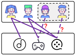
(a) User Cold-Start

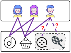
(b) Item Cold-Start

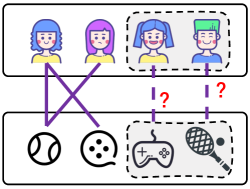
(c) User&Item Cold-Start

Figure 2: Three cold-start scenarios for rating prediction: Entities in dotted boxes are the cold-start entities.

We formulate the problem of cold-start rating prediction, and introduce multi-head self-attention based on which HIRE is developed.

III-A Problem Statement

A recommendation system has a set of users ${\mathcal{U}}=\{u_{1},\cdots,u_{M}\}$ and a set of items ${\mathcal{I}}=\{i_{1},\cdots,i_{N}\}$. The users and items are associated with categorical attributes, i.e., the user profiles and item descriptions. Here, we use $\bm{e}^{k}_{u}$ and $\bm{e}^{k}_{i}$ to denote the $k$-th categorical attribute of a user $u$ and an item $i$, respectively, which are represented by one-hot encoding. We also use $r_{ui}$ to denote the observed rating (preference) of user $u$ to item $i$. Given a set of observed ratings, ${\mathcal{R}}$, rating prediction is to predict unknown rating for pairs of users and items. Table I summarizes the frequently-used notations in this paper.

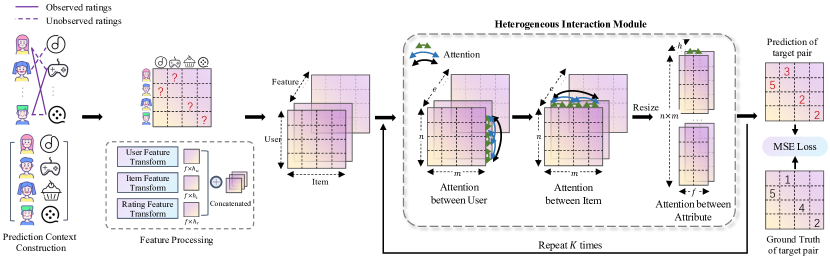
Figure 3: The architecture of HIRE. For ratings of cold user/items to be predicted, HIRE first samples a prediction context. Then, the model constructs the initial embedding for the prediction context and learns the heterogeneous interactions via $K$ HIMs. Finally, the output embedding of the last HIM is transformed into the predicted rating matrix.

Cold-start rating prediction is to predict cold-start users or/and items. There are three scenarios:

• User Cold-Start: The user $u^{*}$ is new arrival, i.e., $u^{*}\notin{\mathcal{U}}$, which has only a few rating interactions with existing items in ${\mathcal{I}}$.

• Item Cold-Start: The item $i^{*}$ is new arrival, i.e., $i^{*}\notin{\mathcal{I}}$, which has only a few rating interactions with existing users in ${\mathcal{U}}$.

• User&Item Cold-Start: Both the user $u^{*}$ and the item $i^{*}$ are new arrival, i.e., $u^{*}\notin{\mathcal{U}}$, $i^{*}\notin{\mathcal{I}}$. They have only a few rating interactions with existing and other possible new items/users in the system.

Fig. 2 shows an example of the three cold-start scenarios in a product rating system, where entities in the dotted boxes are cold-start entities. In Fig. 2(a), it shows a User cold-start scenario to predict two new users’ ratings on three existing items, in Fig. 2(b), it shows an Item cold-start scenario to predict existing users’ preference on two cold items (e.g., movie and tennis racket), and in Fig. 2(c), it shows a User&Item cold-start scenario to predict the ratings of two new users on 2 new items (e.g., game and tennis racket).

Given the user set ${\mathcal{U}}$, item set ${\mathcal{I}}$ and the observed rating ${\mathcal{R}}$, in this paper, we build a deep learning model to support above cold-start rating prediction. It is important to note that by cold-start, the cold user and item to be predicted, as well as their associated ratings, are unavailable in the model training stage.

III-B Multi-Head Self-Attention

Multi-head self-attention (MHSA) [39] is the building block of foundation models, such as BERT [40], GPT [41], Vision Transformer [42], achieving high performance in various natural language processing and computer vision tasks. Given a sequence of tokens $X=[x_{1},\cdots,x_{t}]\in\mathbb{R}^{t\times d}$ as input, self-attention models the interactions among the tokens by computing the attention weights $A\in\mathbb{R}^{t\times t}$ as Eq. (1)-(2). Here, $W_{Q}\in\mathbb{R}^{d\times d^{k}}$, $W_{K}\in\mathbb{R}^{d\times d^{k}}$ are linear weights that map $X$ to query matrix $Q\in\mathbb{R}^{t\times d^{k}}$ and key matrix $K\in\mathbb{R}^{t\times d^{k}}$, respectively, and $A_{ij}$ indicate the similarity between token $x_{i}$ and $x_{j}$.

$$Q=XW_{Q},K=XW_{K}$$ (1)

$$A=\text{softmax}(\frac{QK^{T}}{\sqrt{d^{k}}})$$ (2)

Self-attention (SA) fuses the embedding of the input tokens by taking $A$ as the aggregation weights, where $W_{V}\in\mathbb{R}^{d\times d^{v}}$ is a linear weight matrix.

$$\text{SA}(X)=AXW_{V}$$ (3)

MHSA computes $l$ self-attention independently and concatenates the results as Eq. (4), where the weight $W_{O}\in\mathbb{R}^{l\cdot d^{v}\times d^{o}}$ maps the concatenated dimension $l\cdot d^{v}$ to the output dimension $d^{o}$ and $\|$ is the concatenation operation.

$$\text{MHSA}(X)=[\text{SA}^{(1)}(X)\|\cdots\|\text{SA}^{(l)}(X)]W_{O}$$ (4)

It is worth noting that MHSA is equivariant w.r.t. the permutation of the tokens. Given a permutation function $\Pi_{[1:t]}$ that shuffles the $t$ tokens by an arbitrary order, we have:

$$\Pi_{[1:t]}\circ\text{MHSA}(X)=\text{MHSA}(\Pi_{[1:t]}\circ X)$$ (5)

Our model adopts MHSA as the unique building block, which indicates the power of deep attention layers in modeling heterogeneous relationships for recommendation tasks.

IV Methodology

We propose a DL framework, Heterogeneous Interaction Rating nEtwork (HIRE), for cold-start rating prediction. In this section, we present an overview of HIRE, followed by details on the input construction and the model architecture.

IV-A Overview

The gist of HIRE is to use a simple yet effective mechanism, MHSA, to holistically learn the interactions in three levels, i.e., users, items, and attributes, in an end-to-end, and data-driven fashion. The overall architecture of HIRE is illustrated in Fig. 3. To predict the rating of a user on an item, where either the user or item or both is cold-start, first we generate a prediction context which is composed of the target user/item, together with a set of pertinent users and items. These pertinent users and items are sampled from the user-item bipartite graph by leveraging the rating interaction. We envision that such users and items randomly selected by explicit rating relationships are informative for the cold-start user/item. Second, for a sampled prediction context, we construct a context matrix as the input of the model, which is a 3-dimensional tensor account for the users, items and attributes. The attributes contain individual attributes of users and items, and the observed ratings between the users and items in the context, where the ratings to be predicted are masked. The context matrix is transformed by $K$ Heterogeneous Interaction Module (HIM) blocks, the main component of the HIRE model, followed by a decoder to generate the prediction matrix. In each HIM block, there are three MHSA layers that learn the interactions between different users, different items and different categories of attributes, respectively. Intuitively, as Fig. 4 shows, the three MHSA layers learn via message passing in three complete graphs, where the nodes are the users, items in the context, and the involved attributes, respectively. In the rest of this section, we will elaborate on the details of the construction of the prediction context and the HIM block in § IV-B and § IV-C, respectively.

From the perspective of the prediction task, what a HIRE model does is analogous to inductive matrix completion [43, 44], where Graph Neural Networks are used to model the interactions in a matrix. However, from the perspective of model design, HIRE is different from these GNN-based approaches. For one thing, GNN-based approaches only learn from a single type of rating relationship. For the other thing, the MHSA we use is a flexible specification of GNN layer [45]. As Eq. (2)-(3) shows, self-attention conducts the message passing on a complete graph with a learned ’soft’ adjacency matrix instead of a fixed adjacency matrix.

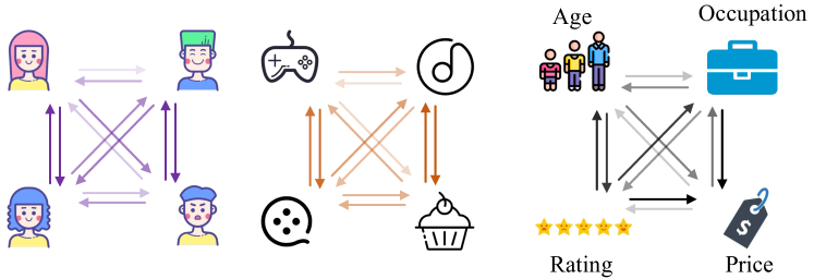
Figure 4: Message Passing in complete graphs via learned interactions

IV-B Construction of Prediction Context

In this section, we delve into the methodology of constructing the prediction context for cold users/items, which encompasses rich information for modeling the heterogeneous interactions to cold users/items. For cold users/items, the prediction context comprises a set of users and items which are relevant to them, associated with their attributes and observed ratings. To determine the relevance of users and items, we employ a neighborhood-based sampling strategy to select the users and items from the user-item interaction bipartite graph. In a nutshell, given the limited budget of $n$ users and $m$ items in a prediction context, our sampling strategy preferentially samples those users/items that have rating interactions with the cold users/items. Concretely, we initialize a seed set by the prediction target, i.e., pairs of users and items involving cold users/items. Subsequently, the sampling begins at the seed set, by selecting the entities of the one-hop neighbors of the seed into the prediction context. If the number of the corresponding neighbor entities does not surpass the current budget, we put all the neighbor entities into the context. Otherwise, a subset of the neighborhood is sampled uniformly subject to the budget size. The neighborhood sampling iterates hop by hop until the budget is exhausted. In § VI-E, we also explore other sampling strategies to construct the context, such as random sampling and feature similarity sampling, where neighbourhood sampling achieves the best empirical results.

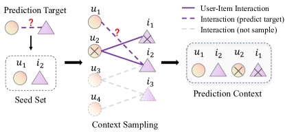
Figure 5: An example of prediction context construction

Fig. 5 shows a toy example of prediction context construction.

Example 1

Given $n=2,m=2$, we aim to predict the rating of a cold user $u_{1}$ on an item $i_{2}$. Initially, the seed set is fixed as $\{u_{1},i_{2}\}$, and an extra user and an extra item need to be sampled. In the bipartite rating graphs in Fig. 5, $i_{2}$ has two neighbors $\{u_{2},u_{3}\}$, in which $u_{2}$ is sampled and the budget for users, $n$, is exhausted. As $u_{1}$ does not have any rated items, we can only sample an item from the neighbors of $u_{2}$, i.e., $i_{1}$. Finally, $\{u_{1},u_{2},i_{1},i_{2}\}$ forms the prediction context.

After sampling $n$ users and $m$ items as the prediction context, we construct a 3-dimensional tensor as the initial input of the model. The tensor, denoted as $\bm{H}\in\mathbb{R}^{n\times m\times e}$, encodes the potential attributes or identities of the users and items and the observed ratings. Concretely, in Eq. (6), the $k$-th row and $j$-th column of $\bm{H}$, $\bm{H}[k,j,\cdot]$, is an $e$-dimensional vector that concatenates three parts of the features, i.e., the features of the user $u_{k}$, $\bm{x}_{u_{k}}$, the features of the item $i_{j}$, $\bm{x}_{i_{j}}$, the vector representation of the potential rating of $u_{k}$ on $i_{j}$, $\bm{x}_{r}$.

$$\bm{H}[k,j,\cdot]\leftarrow[\bm{x}_{u_{k}}\|\bm{x}_{i_{j}}\|\bm{x}_{r}]$$ (6)

The user and item features derive from linear transformation from the original attributes into hidden space. Let $\bm{e}_{u}^{k}$ denotes the one-hot embedding of the $k$-th categorical attribute of a user $u$. For the $h_{u}$ attributes of users, there are $h_{u}$ independent linear transformations $\{f_{U}^{1},\cdots,f_{U}^{h_{u}}\}$ that transforms the one-hot embeddings into hidden features respectively, and the user feature $\bm{x}_{u}$ is the concatenation of those features as shown in Eq. (7). All the users in the recommendation system share the same set of linear feature transformations. And the item feature $\bm{x}_{i}$ is generated in a similar fashion as shown in Eq. (8).

$$\bm{x}_{u} \leftarrow[f_{U}^{1}(\bm{e}_{u}^{1})\|f_{U}^{2}(\bm{e}_{u}^{2})\|\dots\|f_{U}^{h_{u}}(\bm{e}_{u}^{h_{u}})]$$ (7)

$$\bm{x}_{i} \leftarrow[f_{I}^{1}(\bm{e}_{i}^{1})\|f_{I}^{2}(\bm{e}_{i}^{2})\|\dots\|f_{I}^{h_{i}}(\bm{e}_{i}^{h_{i}})]$$ (8)

For the ratings, we also use a linear transformation $f_{R}$ to map the concrete one-hot encoding of a rating $r$, $\bm{e}_{r}$, to the hidden representation $\bm{x}_{r}$ as shown in Eq. (9).

$$\bm{x}_{r}\leftarrow f(\bm{e}_{r})$$ (9)

If the rating $r$ is masked that will be predicted by the model, here, $\bm{e}_{r}$ and $\bm{x}_{r}$ are full-zero vectors. Suppose all the linear transformations $f_{U}^{k}$, $f_{I}^{k}$ and $f_{R}$ map all the one-hot embeddings into $f$-dimensional vectors. The dimension of the feature vector $\bm{H}[k,j,\cdot]$, $e$, equals to $(h_{u}+h_{i}+1)\times f$. If a user/item does not possess an attribute, we set $\bm{e}_{u}$/$\bm{e}_{i}$ to the one-hot encoding of the ID of the user/item as its unique attribute, which is also transformed by a linear mapping $f_{U}$/$f_{I}$. The encoding of $\bm{H}$ can be easily extended to encode continuous attributes and ratings.

IV-C Model Details

We give the technical details of the heterogeneous interaction module (HIM) of HIRE. HIM fully exploits self-attention, a prevailing and powerful neural network layer, to learn implicit interactions. One HIM is composed of three different attention layers, i.e., attention between users, attention between items and attention between attributes, which are stacked layer by layer.

Modeling interactions between users (MBU). Given the initial embedding of the context $\bm{H}\in\mathbb{R}^{n\times m\times e}$, where $n$ is the number of users, $m$ is the number of items, $e$ is the embedding dimension of attributes, we introduce an attention layer between users to model their implicit interactions. Specifically, we use $H_{i_{j}}=\bm{H}[\cdot,j,\cdot]\in\mathbb{R}^{n\times e}$ to denote the embedding view of item $j$ in $\bm{H}$. An item embedding view, $H_{i_{j}}$, is processed by a multi-head self-attention (MHSA) layer, where the attention weights between $n$ users are computed, which is specific to item $j$. In Eq. (10), $\tilde{H}_{i_{j}}\in\mathbb{R}^{m\times e}$ is the fused item embedding view weighted by the attention weights among users. All the item embedding views are processed by a parameter-sharing MHSA in parallel, and the fused embeddings, $\{\tilde{H}_{i_{j}}|j\in[1,m]\}$, are stacked as the output embedding $\bm{H}^{(U)}\in\mathbb{R}^{n\times m\times e}$ (Eq. (11)).

$$\tilde{H}_{i_{j}} \leftarrow\text{MHSA}(H_{i_{j}}),\forall{j}\in[1,\cdots,m]$$ (10)

$$\bm{H}^{(U)} \leftarrow[\tilde{H}_{i_{1}}\|\tilde{H}_{i_{2}}\|\cdots\|\tilde{H}_{i_{m}}]$$ (11)

Modeling interaction between items (MBI). To further model the attention between items, we introduce an attention layer between items, given the stacked output embedding $\bm{H}^{(U)}\in\mathbb{R}^{n\times m\times e}$ as the input. Similarly, ${H}_{u_{k}}=\bm{H}^{(U)}[k,\cdot,\cdot]\in\mathbb{R}^{m\times e}$ denotes the embedding view of user $k$ in $\bm{H}^{(U)}$. The attention weights between $m$ items are computed through a MHSA layer, which is specific to a user embedding view, $H_{u_{k}}$, indicating the user-specific interactions of items. As Eq. (12) shows, $\tilde{H}_{u_{k}}$ is the fused user embedding view weighted by the attention weights among items. A parameter-sharing MHSA processes $m$ independent user embedding views in parallel. The fused embeddings, $\{\tilde{H}_{u_{k}}|k\in[1,n]\}$, are stacked as the output embedding $\bm{H}^{(I)}\in\mathbb{R}^{n\times m\times e}$ (Eq. (13)).

$$\tilde{H}_{u_{k}} \leftarrow\text{MHSA}(H_{u_{k}}),\forall{k}\in[1,\cdots,n]$$ (12)

$$\bm{H}^{(I)} \leftarrow[\tilde{H}_{u_{1}}\|\tilde{H}_{u_{2}}\|\cdots\|\tilde{H}_{u_{n}}]$$ (13)

Modeling interaction between attributes (MBA). HIM further learns the interaction between fine-grained attributes by computing the attention between user and item attributes. Taking the embedding $\bm{H}^{(I)}\in\mathbb{R}^{n\times m\times e}$ as input, we first reshape $\bm{H}^{(I)}$ to $\mathbb{R}^{n\times m\times h\times f}$ by spliting the feature dimension $e$ into $h\times f$, where $h$ is the number of categorical attributes and $f$ is the embedding dimension for each attribute. We use ${H}_{u_{k},i_{j}}=\bm{H}^{(I)}[k,j,\cdot,\cdot]\in\mathbb{R}^{h\times f}$ to denote the embedding view of a user-item pair $(u_{k},i_{j})$ in $\bm{H}^{(I)}$. The embedding view $H_{u_{k},i_{j}}$ is processed by a MHSA layer, where the attention weights between $h$ attributes are computed, indicating the interaction between attributes that is specific to a user-item pair $(u_{k},i_{j})$. $\tilde{H}_{u_{k},i_{j}}\in\mathbb{R}^{h\times f}$ in Eq. (14) is the fused user-item pair embedding view weighted by the attention weights between the $h$ attributes. All the user-item pair embedding views are processed by a parameter-sharing MHSA in parallel, and the fused embeddings, $\{\tilde{H}_{u_{k},i_{j}}|k\in[1,n],j\in[1,m]\}$, are stacked as the output embedding $\bm{H}^{(A)}\in\mathbb{R}^{n\times m\times h\times f}$ (Eq. (15)). The embedding $\bm{H}^{(A)}$ will be reshaped to $\mathbb{R}^{n\times m\times e}$ by flatting the feature dimension $h\times f$ back to $e$ for future processing.

$$\tilde{H}_{u_{k},i_{j}} \leftarrow\text{MHSA}(H_{u_{k},i_{j}}),\forall{k}\in[1,\cdots,n],\forall{j}\in[1,\cdots,m]$$ (14)

$$\bm{H}^{(A)}\leftarrow[\tilde{H}_{u_{1},i_{1}}\|\tilde{H}_{u_{1},i_{2}}\|\cdots\|\tilde{H}_{u_{1},i_{m}}$$

$$\tilde{H}_{u_{2},i_{1}}\|\tilde{H}_{u_{2},i_{2}}\|\cdots\|\tilde{H}_{u_{2},i_{m}}$$

$$\cdots$$

$$\tilde{H}_{u_{n},i_{1}}\|\tilde{H}_{u_{n},i_{2}}\|\cdots\|\tilde{H}_{u_{n},i_{m}}]$$ (15)

To summarize, HIM takes the sampled context $\bm{H}\in\mathbb{R}^{n\times m\times e}$ as input embedding, and model the interactions between users, items and attributes by three MHSA layer by layer. It finally generates embedding $\bm{H}^{(A)}\in\mathbb{R}^{n\times m\times e}$ which adaptively aggregates the features of users, items and attributes in the context by leveraging the attention weights. As Fig. 3 presents, the model HIRE is composed of $K$ HIMs, where the output of the $(k-1)$-th HIM is fed into $k$-th HIM for modeling the higher order interactions.

Rating Prediction. Given $\bm{H}^{(A)}\in\mathbb{R}^{n\times m\times e}$ as the output of the $K$-th HIM, we use a decoder to predict the rating matrix $\hat{R}\in\mathbb{R}^{n\times m}$ of the sampled context as Eq. (16).

$$\hat{R}\leftarrow\alpha\cdot\text{Sigmoid}(g_{\theta}(\bm{H}^{(A)}))$$ (16)

Here, $g_{\theta}:\mathbb{R}^{e}\rightarrow\mathbb{R}^{1}$ is a linear transformation parameterized by $\theta$ and $\alpha\in\mathbb{R}$ is a scalar that rescales the range of the estimated ratings.

V Model Training and Analysis

In this section, we further present the training of HIRE and analyze the complexity and inductive bias of the model.

V-A Model Training

In a recommendation system, given a set of users ${\mathcal{U}}$, a set of items ${\mathcal{I}}$ and observed ratings ${\mathcal{R}}$, a HIRE model is trained by a set of prediction contexts, denoted as $\mathcal{D}$, which are sampled from ${\mathcal{U}}$, ${\mathcal{I}}$, and ${\mathcal{R}}$. Given a ratio of $p$ ratings in a prediction context, the model is optimized to minimize the mean squared error (MSE) loss (Eq. (17)) for the $1-p$ of masked ratings.

$$\mathcal{L}=\frac{1}{|\mathcal{D}|}\sum_{\mathcal{D}}\frac{1}{|\mathcal{Q}|}\sum_{r\in\mathcal{Q}}\norm{r-\hat{r}}^{2}$$ (17)

where $\hat{r}\in\mathbb{R}$ is a predicted rating in the output matrix $\hat{R}$ and $r\in\mathbb{R}$ is the corresponding ground truth rating. We use $\mathcal{Q}$ to denote the masked rating set.

Algorithm 1 presents the training process implemented by stochastic gradient descent. In each step, we randomly draw a mini-batch of prediction context, $\mathcal{B}$, from the training set $\mathcal{D}$ as line 1. Then, in line 1-1, each context is transformed by the three attention layers in a HIM block one by one, and there are $K$ HIM blocks in total. In line 1, the output of the $K$-th HIM is mapped to the predicted rating matrix $\hat{R}$. Finally, we compute the MSE Loss for the mini-batch $\mathcal{B}$ and update the model parameters via the back-propagation of gradient in line 1-1. The training will be terminated until the MSE loss converges.

In test stage, when new user set $\mathcal{U}^{*}$ and item set $\mathcal{I}^{*}$ comes, we can construct an embedding matrix $\bm{H}^{*}$. Ratings to be predicted are masked. It is worth to mention that the size of matrix can be decided by the number of new users and items and can be flexible. $\bm{H}^{*}$ is input into $K$ HIM blocks following a mapping function to get predicted rating.

V-B Model Analysis

We analyze the time and space complexity of HIRE in brief. Suppose a prediction context is composed of $n$ users and $m$ items. $e=h\times f$ is the hidden dimension of the MHSA layer in HIM, where $h$ is the number of attributes and $f$ is the embedding dimension of each attribute. The linear feature transformation of HIRE (Eq. (7)-(9)) takes ${\mathcal{O}}(nmee_{0})$ time, where $e_{0}$ is the maximum dimension of original feature. The computation of HIM dominates the complexity of HIRE. Specifically, the time complexities of the attention between users (Eq. (10)-(11)), attention between items (Eq. (12)-(13)) and attention between attributes (Eq. (14)-(15)) are ${\mathcal{O}}(n^{2}me)$, ${\mathcal{O}}(nm^{2}e)$, ${\mathcal{O}}(nmh^{2}f)$, respectively. The time complexity of the output layer (Eq. (16)) for rating prediction is $\mathcal{O}(nme)$. Assume $e_{0}\ll e$ and the model is composed of $K$ HIM blocks, the total time complexity is ${\mathcal{O}}(Knme(n+m+h))$. Regarding the space complexity, our neighborhood-based sampling strategy constructs a matrix which costs $\mathcal{O}(nme_{0})$ space complexity for each task. For attention between users, items and attributes, the space complexity is $\mathcal{O}(n^{2}me)$, $\mathcal{O}(nm^{2}e)$ and $\mathcal{O}(nmh^{2}f)$, respectively. Thus the total space complexity for one context is $\mathcal{O}(Knme(n+m+h))$.

In addition, HIRE preserves an inherent inductive bias when exploiting sets of users and items for rating prediction, which is formulated as the property below.

Property 5.1. Given a set of users $\{u_{1},\cdots,u_{n}\}$ and a set of items $\{i_{1},\cdots,i_{m}\}$ as a prediction context $\bm{H}$ and the HIRE model $\mathcal{M}$, the predicted rating matrix, $\hat{R}$, is equivariant w.r.t. any permutation of the user set $\Pi_{[1:n]}$ and permutation of the item set $\Pi_{[1:m]}$.

$$\Pi_{[1:n]}\circ\Pi_{[1:m]}\circ\hat{R}=\mathcal{M}(\Pi_{[1:n]}\circ\Pi_{[1:m]}\circ\bm{H})$$ (18)

The inductive bias is intuitive, since the MHSA is permutation equivariant., i.e.,

$$\Pi_{[1:n]}\circ\tilde{H}_{i_{j}} \leftarrow\text{MHSA}(\Pi_{[1:n]}\circ H_{i_{j}})$$ (19)

$$\Pi_{[1:m]}\circ\tilde{H}_{u_{k}} \leftarrow\text{MHSA}(\Pi_{[1:m]}\circ H_{u_{k}})$$ (20)

And matrices stack/concatenation naturally preserve permutation equivariance. This property ensures that given the sets of users and items in the prediction context, our model predicts deterministic ratings regardless their input order, which also shows that our approach can make use of MHSA designed for sequential inputs to solve the cold-start problem.

Input : User set $\mathcal{U}$, item set $\mathcal{I}$, observed ratings $\mathcal{R}$.

Output : Model parameters.

1

2Initialize model parameters;

3 Generate a set of context matrices $\mathcal{D}=\{\bm{H}_{1},\cdots\}$ for training;

4 do

5       Sample a mini-batch of context matrices $\mathcal{B}\sim\mathcal{D}$;

6       for $\bm{H}\in\mathcal{B}$ do

7             for $k\rightarrow 1$ to $K$ do

8                   Compute $\bm{H}^{(U)}$ via Eq. (10)-(11);

9                   Compute $\bm{H}^{(I)}$ via Eq. (12)-(13);

10                   Compute $\bm{H}^{(A)}$ via Eq. (14)-(15);

11                  

12             end for

13            Compute the predicted rating matrix $\hat{R}$ via Eq. (16);

14            

15       end for

16      Compute the MSE Loss $\mathcal{L}$ via Eq. (17);

17       Update model parameters by gradient descent;

18      

19while $\mathcal{L}$ converges

Algorithm 1 Training Algorithm of HIRE

TABLE II: Profile of Datasets

Dataset	$\mathsf{MovieLens}$-$\mathsf{1M}$	$\mathsf{Douban}$	$\mathsf{Bookcrossing}$
# Users	6,040	23,822	278,858
# Items	3,706	185,574	271,379
# Ratings	1,000,209	1,387,216	1,149,780
User Attributes	Age, Occupation, Gender, Zip code	N/A	Age
Item Attributes	Rate, Genre, Director, Actor	N/A	Publication year
Range of Ratings	$1\sim 5$	$1\sim 5$	$1\sim 10$

TABLE III: Overall Performance in Three Cold-Start Scenarios on $\mathsf{MovieLens}$-$\mathsf{1M}$

Scenarios	Methods	TOP5			TOP7			TOP10
		Precision	NDCG	MAP	Precision	NDCG	MAP	Precision	NDCG	MAP
UC	NeuMF	$0.4702_{\small(.0066)}$	$0.7073_{\small(.0034)}$	$0.3713_{\small(.0068)}$	$0.5026_{\small(.0067)}$	$0.6899_{\small(.0045)}$	$0.3947_{\small(.0063)}$	$0.5478_{\small(.0065)}$	$0.6713_{\small(.0052)}$	$0.4391_{\small(.0068)}$
	Wide&Deep	$0.5189_{\small(.0083)}$	$0.8385_{\small(.0015)}$	$0.4157_{\small(.0102)}$	$0.5561_{\small(.0047)}$	$0.8396_{\small(.0021)}$	$0.4420_{\small(.0058)}$	$0.6248_{\small(.0066)}$	$0.8471_{\small(.0015)}$	$0.5081_{\small(.0093)}$
	DeepFM	$0.5169_{\small(.0092)}$	$0.8367_{\small(.0079)}$	$0.4123_{\small(.0093)}$	$0.5536_{\small(.0053)}$	$0.8385_{\small(.0073)}$	$0.4384_{\small(.0062)}$	$0.6190_{\small(.0025)}$	$0.8451_{\small(.0063)}$	$0.5019_{\small(.0028)}$
	AFN	$0.5084_{\small(.0057)}$	$0.8294_{\small(.0032)}$	$0.3998_{\small(.0056)}$	$0.5550_{\small(.0033)}$	$0.8333_{\small(.0029)}$	$0.4340_{\small(.0033)}$	$0.6254_{\small(.0026)}$	$0.8423_{\small(.0018)}$	$0.5028_{\small(.0043)}$
	GraphHINGE	$0.5180_{\small(.0075)}$	$0.7809_{\small(.0058)}$	$0.4076_{\small(.0071)}$	$0.5819_{\small(.0086)}$	$0.7787_{\small(.0066)}$	$0.4655_{\small(.0086)}$	$0.6462_{\small(.0076)}$	$0.7752_{\small(.0064)}$	$0.5303_{\small(.0094)}$
	MetaHIN	$0.4392_{\small(.0238)}$	$0.8005_{\small(.0107)}$	$0.3579_{\small(.0245)}$	$0.4892_{\small(.0162)}$	$0.8109_{\small(.0092)}$	$0.3881_{\small(.0179)}$	$0.5644_{\small(.0148)}$	$0.8258_{\small(.0091)}$	$0.4572_{\small(.0191)}$
	MAMO	$0.4663_{\small(.0053)}$	$0.5905_{\small(.0079)}$	$0.3405_{\small(.0070)}$	$0.5294_{\small(.0038)}$	$0.6119_{\small(.0062)}$	$0.3869_{\small(.0032)}$	$0.6466_{\small(.0063)}$	$0.6531_{\small(.0032)}$	$0.5086_{\small(.0040)}$
	TaNP	$0.5715_{\small(.0102)}$	$0.8718_{\small(.0041)}$	$0.4728_{\small(.0099)}$	$0.5986_{\small(.0044)}$	$0.8731_{\small(.0026)}$	$0.4899_{\small(.0069)}$	$0.6591_{\small(.0049)}$	$0.8807_{\small(.0020)}$	$0.5495_{\small(.0054)}$
	MeLU	$0.5093_{\small(.0066)}$	$0.6254_{\small(.0173)}$	$0.4011_{\small(.0149)}$	$0.5787_{\small(.0018)}$	$0.6499_{\small(.0129)}$	$0.4622_{\small(.0107)}$	$0.6882_{\small(.0149)}$	$0.6974_{\small(.0139)}$	$0.5767_{\small(.0167)}$
	HIRE	$\mathbf{0.6999_{\small(.0184)}}$	$\mathbf{0.9169_{\small(.0145)}}$	$\mathbf{0.6454_{\small(.0309)}}$	$\mathbf{0.7259_{\small(.0042)}}$	$\mathbf{0.9254_{\small(.0176)}}$	$\mathbf{0.6652_{\small(.0144)}}$	$\mathbf{0.7656_{\small(.0246)}}$	$\mathbf{0.9432_{\small(.0223)}}$	$\mathbf{0.7065_{\small(.0211)}}$
IC	NeuMF	$0.5726_{\small(.0062)}$	$0.7503_{\small(.0045)}$	$0.4982_{\small(.0061)}$	$0.6097_{\small(.0062)}$	$0.7353_{\small(.0048)}$	$0.5356_{\small(.0062)}$	$0.6609_{\small(.0063)}$	$0.7237_{\small(.0055)}$	$0.5933_{\small(.0061)}$
	Wide&Deep	$0.3006_{\small(.0111)}$	$0.5196_{\small(.0614)}$	$0.1925_{\small(.0174)}$	$0.3751_{\small(.0196)}$	$0.5407_{\small(.0603)}$	$0.2373_{\small(.0328)}$	$0.4681_{\small(.0301)}$	$0.5635_{\small(.0583)}$	$0.3090_{\small(.0533)}$
	DeepFM	$0.3091_{\small(.0015)}$	$0.5309_{\small(.0649)}$	$0.2012_{\small(.0090)}$	$0.3795_{\small(.0143)}$	$0.5486_{\small(.0609)}$	$0.2451_{\small(.0247)}$	$0.4672_{\small(.0342)}$	$0.5689_{\small(.0537)}$	$0.3134_{\small(.0506)}$
	AFN	$0.2989_{\small(.0256)}$	$0.4855_{\small(.0878)}$	$0.1891_{\small(.0057)}$	$0.3705_{\small(.0126)}$	$0.5111_{\small(.0856)}$	$0.2308_{\small(.0089)}$	$0.4592_{\small(.0128)}$	$0.5387_{\small(.0780)}$	$0.2965_{\small(.0338)}$
	GraphHINGE	$0.1428_{\small(.0037)}$	$0.1779_{\small(.0072)}$	$0.0567_{\small(.0017)}$	$0.2087_{\small(.0058)}$	$0.2214_{\small(.0083)}$	$0.0769_{\small(.0027)}$	$0.2971_{\small(.0050)}$	$0.2670_{\small(.0092)}$	$0.1148_{\small(.0019)}$
	MetaHIN	$0.4369_{\small(.0144)}$	$0.7941_{\small(.0068)}$	$0.3541_{\small(.0159)}$	$0.4934_{\small(.0098)}$	$0.8044_{\small(.0054)}$	$0.3917_{\small(.0122)}$	$0.5624_{\small(.0074)}$	$0.8196_{\small(.0052)}$	$0.4489_{\small(.0106)}$
	MAMO	$0.4687_{\small(.0132)}$	$0.5942_{\small(.0090)}$	$0.3439_{\small(.0080)}$	$0.5425_{\small(.0023)}$	$0.6194_{\small(.0064)}$	$0.4006_{\small(.0009)}$	$0.6515_{\small(.0040)}$	$0.6590_{\small(.0044)}$	$0.5152_{\small(.0085)}$
	TaNP	$0.4068_{\small(.0122)}$	$0.7564_{\small(.0060)}$	$0.2720_{\small(.0152)}$	$0.4882_{\small(.0155)}$	$0.7741_{\small(.0065)}$	$0.3339_{\small(.0202)}$	$0.5938_{\small(.0207)}$	$0.7982_{\small(.0077)}$	$0.4383_{\small(.0290)}$
	MeLU	$0.4893_{\small(.0079)}$	$0.5920_{\small(.0126)}$	$0.3666_{\small(.0172)}$	$0.5708_{\small(.0067)}$	$0.6244_{\small(.0058)}$	$0.4397_{\small(.0035)}$	$0.6860_{\small(.0178)}$	$0.6761_{\small(.0039)}$	$0.5665_{\small(.0139)}$
	HIRE	$\mathbf{0.5989_{\small(.0161)}}$	$\mathbf{0.8640_{\small(.0162)}}$	$\mathbf{0.5304_{\small(.0307)}}$	$\mathbf{0.6444_{\small(.0116)}}$	$\mathbf{0.8750_{\small(.0188)}}$	$\mathbf{0.5672_{\small(.0186)}}$	$\mathbf{0.7125_{\small(.0284)}}$	$\mathbf{0.8987_{\small(.0222)}}$	$\mathbf{0.6372_{\small(.0260)}}$
U&I C	NeuMF	$0.5599_{\small(.0061)}$	$0.7059_{\small(.0062)}$	$0.4850_{\small(.0064)}$	$0.6065_{\small(.0053)}$	$0.6936_{\small(.0062)}$	$0.5326_{\small(.0054)}$	$0.6682_{\small(.0036)}$	$0.6885_{\small(.0057)}$	$0.6034_{\small(.0039)}$
	Wide&Deep	$0.2952_{\small(.0128)}$	$0.5113_{\small(.0610)}$	$0.1857_{\small(.0179)}$	$0.3745_{\small(.0241)}$	$0.5345_{\small(.0586)}$	$0.2337_{\small(.0353)}$	$0.4663_{\small(.0348)}$	$0.5577_{\small(.0559)}$	$0.3039_{\small(.0578)}$
	DeepFM	$0.3099_{\small(.0073)}$	$0.5286_{\small(.0674)}$	$0.1971_{\small(.0058)}$	$0.3870_{\small(.0074)}$	$0.5467_{\small(.0638)}$	$0.2474_{\small(.0220)}$	$0.4691_{\small(.0330)}$	$0.5651_{\small(.0557)}$	$0.3121_{\small(.0523)}$
	AFN	$0.2918_{\small(.0290)}$	$0.4749_{\small(.0916)}$	$0.1828_{\small(.0098)}$	$0.3674_{\small(.0183)}$	$0.5016_{\small(.0911)}$	$0.2285_{\small(.0043)}$	$0.4584_{\small(.0116)}$	$0.5317_{\small(.0818)}$	$0.2912_{\small(.0347)}$
	GraphHINGE	$0.0992_{\small(.0045)}$	$0.1131_{\small(.0062)}$	$0.0335_{\small(.0018)}$	$0.1700_{\small(.0032)}$	$0.1567_{\small(.0055)}$	$0.0552_{\small(.0015)}$	$0.2913_{\small(.0034)}$	$0.2078_{\small(.0043)}$	$0.1248_{\small(.0042)}$
	MetaHIN	$0.4392_{\small(.0238)}$	$0.8005_{\small(.0107)}$	$0.3579_{\small(.0245)}$	$0.4892_{\small(.0162)}$	$0.8109_{\small(.0092)}$	$0.3881_{\small(.0179)}$	$0.5644_{\small(.0148)}$	$0.8258_{\small(.0091)}$	$0.4572_{\small(.0191)}$
	MAMO	$0.4789_{\small(.0053)}$	$0.6046_{\small(.0001)}$	$0.3550_{\small(.0020)}$	$0.5391_{\small(.0062)}$	$0.6251_{\small(.0018)}$	$0.3971_{\small(.0026)}$	$0.6480_{\small(.0013)}$	$0.6614_{\small(.0028)}$	$0.5120_{\small(.0069)}$
	TaNP	$0.4114_{\small(.0112)}$	$0.7663_{\small(.0051)}$	$0.2813_{\small(.0093)}$	$0.4929_{\small(.0100)}$	$0.7820_{\small(.0042)}$	$0.3441_{\small(.0066)}$	$0.5867_{\small(.0074)}$	$0.8016_{\small(.0024)}$	$0.4335_{\small(.0096)}$
	MeLU	$0.4680_{\small(.0103)}$	$0.5692_{\small(.0060)}$	$0.3393_{\small(.0055)}$	$0.5616_{\small(.0126)}$	$0.6087_{\small(.0072)}$	$0.4210_{\small(.0128)}$	$0.6840_{\small(.0179)}$	$0.6650_{\small(.0094)}$	$0.5556_{\small(.0232)}$
	HIRE	$\mathbf{0.6030_{\small(.0175)}}$	$\mathbf{0.8693_{\small(.0180)}}$	$\mathbf{0.5362_{\small(.0319)}}$	$\mathbf{0.6627_{\small(.0073)}}$	$\mathbf{0.8837_{\small(.0207)}}$	$\mathbf{0.5904_{\small(.0116)}}$	$\mathbf{0.7419_{\small(.0429)}}$	$\mathbf{0.9140_{\small(.0233)}}$	$\mathbf{0.6764_{\small(.0433)}}$

TABLE IV: Overall Performance in Three Cold-Start Scenarios on $\mathsf{Bookcrossing}$

Scenarios	Methods	TOP5			TOP7			TOP10
		Precision	NDCG	MAP	Precision	NDCG	MAP	Precision	NDCG	MAP
UC	NeuMF	$0.3328_{\small(.0106)}$	$0.3887_{\small(.0110)}$	$0.2657_{\small(.0167)}$	$0.4176_{\small(.0112)}$	$0.3962_{\small(.0132)}$	$0.3388_{\small(.0203)}$	$0.5165_{\small(.0155)}$	$0.4178_{\small(.0127)}$	$0.4214_{\small(.0271)}$
	Wide&Deep	$0.2852_{\small(.0161)}$	$0.5408_{\small(.0197)}$	$0.2161_{\small(.0008)}$	$0.3759_{\small(.0231)}$	$0.5528_{\small(.0273)}$	$0.2517_{\small(.0196)}$	$0.4746_{\small(.0678)}$	$0.5666_{\small(.0416)}$	$0.3258_{\small(.0504)}$
	DeepFM	$0.2956_{\small(.0013)}$	$0.5154_{\small(.0066)}$	$0.1870_{\small(.0079)}$	$0.3511_{\small(.0125)}$	$0.5230_{\small(.0151)}$	$0.2120_{\small(.0070)}$	$0.4321_{\small(.0278)}$	$0.5224_{\small(.0015)}$	$0.2787_{\small(.0233)}$
	AFN	$0.2205_{\small(.0714)}$	$0.4970_{\small(.0354)}$	$0.1462_{\small(.0644)}$	$0.3195_{\small(.0414)}$	$0.5063_{\small(.0264)}$	$0.1856_{\small(.0452)}$	$0.4210_{\small(.0066)}$	$0.5238_{\small(.0080)}$	$0.2573_{\small(.0277)}$
	MAMO	$0.4016_{\small(.0115)}$	$0.2752_{\small(.0194)}$	$0.3062_{\small(.0123)}$	$0.5444_{\small(.0070)}$	$0.3244_{\small(.0184)}$	$0.4419_{\small(.0091)}$	$0.7119_{\small(.0046)}$	$0.3895_{\small(.0150)}$	$0.6417_{\small(.0065)}$
	TaNP	$0.4118_{\small(.0030)}$	$0.8504_{\small(.0145)}$	$0.3338_{\small(.0039)}$	$0.4598_{\small(.0054)}$	$0.8601_{\small(.0110)}$	$0.3626_{\small(.0131)}$	$0.5288_{\small(.0210)}$	$0.8712_{\small(.0072)}$	$0.4160_{\small(.0329)}$
	MeLU	$0.4651_{\small(.0416)}$	$0.5860_{\small(.0709)}$	$0.3534_{\small(.0440)}$	$0.5282_{\small(.0779)}$	$0.6079_{\small(.0737)}$	$0.4079_{\small(.0662)}$	$0.6701_{\small(.0442)}$	$0.6466_{\small(.0798)}$	$0.5558_{\small(.0492)}$
	HIRE	$\mathbf{0.5713_{\small(.0530)}}$	$\mathbf{0.8931_{\small(.0291)}}$	$\mathbf{0.5079_{\small(.0751)}}$	$\mathbf{0.6405_{\small(.0257)}}$	$\mathbf{0.9058_{\small(.0267)}}$	$\mathbf{0.5640_{\small(.0544)}}$	$\mathbf{0.7191_{\small(.0284)}}$	$\mathbf{0.9295_{\small(.0234)}}$	$\mathbf{0.6475_{\small(.0151)}}$
IC	NeuMF	$0.4070_{\small(.0066)}$	$0.3632_{\small(.0407)}$	$0.3282_{\small(.0414)}$	$0.5142_{\small(.0225)}$	$0.3813_{\small(.0422)}$	$0.4303_{\small(.0773)}$	$0.5930_{\small(.0868)}$	$0.4103_{\small(.0430)}$	$0.5729_{\small(.0200)}$
	Wide&Deep	$0.5007_{\small(.0786)}$	$0.8014_{\small(.0095)}$	$0.3814_{\small(.0935)}$	$0.5451_{\small(.0885)}$	$0.8059_{\small(.0096)}$	$0.3953_{\small(.0874)}$	$0.5870_{\small(.0914)}$	$0.8047_{\small(.0058)}$	$0.4393_{\small(.0928)}$
	DeepFM	$0.5246_{\small(.0813)}$	$0.8110_{\small(.0162)}$	$0.4092_{\small(.0772)}$	$0.5142_{\small(.0723)}$	$0.8156_{\small(.0181)}$	$0.4121_{\small(.0928)}$	$0.5515_{\small(.0769)}$	$0.8123_{\small(.0219)}$	$0.4437_{\small(.0995)}$
	AFN	$0.4915_{\small(.0710)}$	$0.8018_{\small(.0178)}$	$0.4040_{\small(.0908)}$	$0.5395_{\small(.0998)}$	$0.8083_{\small(.0187)}$	$0.3764_{\small(.0761)}$	$0.5679_{\small(.0660)}$	$0.8129_{\small(.0187)}$	$0.4399_{\small(.0891)}$
	MAMO	$0.4129_{\small(.0062)}$	$0.2810_{\small(.0049)}$	$0.3246_{\small(.0051)}$	$0.5462_{\small(.0041)}$	$0.3240_{\small(.0036)}$	$0.4498_{\small(.0071)}$	$0.7160_{\small(.0036)}$	$0.3942_{\small(.0086)}$	$0.6418_{\small(.0019)}$
	TaNP	$0.4116_{\small(.0315)}$	$0.8545_{\small(.0132)}$	$0.3125_{\small(.0152)}$	$0.4506_{\small(.0174)}$	$0.8618_{\small(.0129)}$	$0.3287_{\small(.0290)}$	$0.5194_{\small(.0435)}$	$0.8713_{\small(.0122)}$	$0.3848_{\small(.0504)}$
	MeLU	$0.4925_{\small(.0577)}$	$0.6159_{\small(.0289)}$	$0.3764_{\small(.0517)}$	$0.5204_{\small(.0820)}$	$0.6258_{\small(.0245)}$	$0.3915_{\small(.0639)}$	$0.6415_{\small(.0872)}$	$0.6565_{\small(.0362)}$	$0.5341_{\small(.0789)}$
	HIRE	$\mathbf{0.5837_{\small(.0338)}}$	$\mathbf{0.8925_{\small(.0056)}}$	$\mathbf{0.5174_{\small(.0327)}}$	$\mathbf{0.6418_{\small(.0244)}}$	$\mathbf{0.9057_{\small(.0057)}}$	$\mathbf{0.5649_{\small(.0206)}}$	$\mathbf{0.7220_{\small(.0471)}}$	$\mathbf{0.9262_{\small(.0065)}}$	$\mathbf{0.6519_{\small(.0497)}}$
U&I C	NeuMF	$0.3829_{\small(.0097)}$	$0.4221_{\small(.0329)}$	$0.2976_{\small(.0105)}$	$0.4342_{\small(.0120)}$	$0.4304_{\small(.0345)}$	$0.3274_{\small(.0229)}$	$0.4922_{\small(.0074)}$	$0.4364_{\small(.0205)}$	$0.3661_{\small(.0170)}$
	Wide&Deep	$0.4037_{\small(.0841)}$	$0.7387_{\small(.0776)}$	$0.3304_{\small(.0696)}$	$0.5023_{\small(.0682)}$	$0.7172_{\small(.0840)}$	$0.4058_{\small(.0692)}$	$0.5649_{\small(.0654)}$	$0.7204_{\small(.0790)}$	$0.3126_{\small(.0866)}$
	DeepFM	$0.3927_{\small(.0771)}$	$0.6848_{\small(.0731)}$	$0.3018_{\small(.0710)}$	$0.4750_{\small(.0294)}$	$0.6900_{\small(.0838)}$	$0.3649_{\small(.0429)}$	$0.5414_{\small(.0965)}$	$0.7266_{\small(.0503)}$	$0.3881_{\small(.0981)}$
	AFN	$0.3476_{\small(.0396)}$	$0.6344_{\small(.0479)}$	$0.2815_{\small(.0301)}$	$0.3505_{\small(.0193)}$	$0.6298_{\small(.0468)}$	$0.2651_{\small(.0085)}$	$0.3988_{\small(.0317)}$	$0.6458_{\small(.0479)}$	$0.2839_{\small(.0289)}$
	MAMO	$0.4100_{\small(.0087)}$	$0.3256_{\small(.0632)}$	$0.3026_{\small(.0376)}$	$0.5167_{\small(.0763)}$	$0.3699_{\small(.0534)}$	$0.4101_{\small(.0934)}$	$0.7178_{\small(.0154)}$	$0.4485_{\small(.0724)}$	$0.6380_{\small(.0391)}$
	TaNP	$0.5114_{\small(.0174)}$	$0.8812_{\small(.0650)}$	$0.4365_{\small(.0083)}$	$0.5153_{\small(.0214)}$	$0.8774_{\small(.0447)}$	$0.4286_{\small(.0456)}$	$0.5484_{\small(.0676)}$	$0.8780_{\small(.0250)}$	$0.4531_{\small(.0856)}$
	MeLU	$0.4335_{\small(.0436)}$	$0.5465_{\small(.0146)}$	$0.3349_{\small(.0293)}$	$0.4992_{\small(.0928)}$	$0.5716_{\small(.0080)}$	$0.3784_{\small(.0788)}$	$0.6373_{\small(.0918)}$	$0.5993_{\small(.0351)}$	$0.5350_{\small(.0999)}$
	HIRE	$\mathbf{0.6077_{\small(.0333)}}$	$\mathbf{0.9060_{\small(.0025)}}$	$\mathbf{0.5529_{\small(.0322)}}$	$\mathbf{0.6903_{\small(.0430)}}$	$\mathbf{0.9209_{\small(.0051)}}$	$\mathbf{0.6284_{\small(.0405)}}$	$\mathbf{0.7636_{\small(.0689)}}$	$\mathbf{0.9392_{\small(.0064)}}$	$\mathbf{0.7015_{\small(.0812)}}$

TABLE V: Overall Performance in Three Cold-Start Scenarios on $\mathsf{Douban}$

Scenarios	Methods	TOP5			TOP7			TOP10
		Precision	NDCG	MAP	Precision	NDCG	MAP	Precision	NDCG	MAP
UC	NeuMF	$0.4443_{\small(.0160)}$	$0.3334_{\small(.0199)}$	$0.4056_{\small(.0164)}$	$0.5872_{\small(.0124)}$	$0.3471_{\small(.0191)}$	$0.5623_{\small(.0130)}$	$0.7261_{\small(.0071)}$	$0.3765_{\small(.0168)}$	$0.7113_{\small(.0080)}$
	Wide&Deep	$0.5442_{\small(.0105)}$	$0.7725_{\small(.0083)}$	$0.4443_{\small(.0175)}$	$0.5566_{\small(.0031)}$	$0.7595_{\small(.0081)}$	$0.4501_{\small(.0120)}$	$0.5826_{\small(.0032)}$	$0.7376_{\small(.0070)}$	$0.4783_{\small(.0068)}$
	DeepFM	$0.5133_{\small(.0178)}$	$0.7261_{\small(.0242)}$	$0.4141_{\small(.0250)}$	$0.5133_{\small(.0239)}$	$0.7016_{\small(.0293)}$	$0.4115_{\small(.0280)}$	$0.5281_{\small(.0147)}$	$0.6707_{\small(.0286)}$	$0.4312_{\small(.0193)}$
	AFN	$0.5918_{\small(.0119)}$	$0.8041_{\small(.0171)}$	$0.4919_{\small(.0198)}$	$0.6088_{\small(.0083)}$	$0.7981_{\small(.0182)}$	$0.4992_{\small(.0157)}$	$0.6442_{\small(.0108)}$	$0.7875_{\small(.0198)}$	$0.5407_{\small(.0038)}$
	GraphRec	$0.6065_{\small(.0279)}$	$0.5073_{\small(.0366)}$	$0.5477_{\small(.0326)}$	$\mathbf{0.7549_{\small(.0238)}}$	$0.5605_{\small(.0373)}$	$\mathbf{0.7220_{\small(.0267)}}$	$\mathbf{0.8771_{\small(.0172)}}$	$0.6206_{\small(.0356)}$	$\mathbf{0.8631_{\small(.0189)}}$
	MAMO	$0.6098_{\small(.0007)}$	$0.7356_{\small(.0005)}$	$0.5101_{\small(.0005)}$	$0.6796_{\small(.0005)}$	$0.7594_{\small(.0002)}$	$0.5741_{\small(.0004)}$	$0.8006_{\small(.0003)}$	$0.8060_{\small(.0002)}$	$0.7209_{\small(.0004)}$
	TaNP	$0.6408_{\small(.0340)}$	$0.9020_{\small(.0104)}$	$0.5465_{\small(.0447)}$	$0.6906_{\small(.0308)}$	$0.9100_{\small(.0094)}$	$0.5919_{\small(.0422)}$	$0.7824_{\small(.0386)}$	$0.9259_{\small(.0104)}$	$0.7044_{\small(.0530)}$
	MeLU	$0.4542_{\small(.0480)}$	$0.6452_{\small(.0181)}$	$0.3463_{\small(.0457)}$	$0.5054_{\small(.0706)}$	$0.6623_{\small(.0269)}$	$0.3815_{\small(.0693)}$	$0.5953_{\small(.0798)}$	$0.6930_{\small(.0352)}$	$0.4723_{\small(.0885)}$
	HIRE	$\mathbf{0.7152_{\small(.0391)}}$	$\mathbf{0.9269_{\small(.0131)}}$	$\mathbf{0.6595_{\small(.0574)}}$	$0.7459_{\small(.0248)}$	$\mathbf{0.9328_{\small(.0122)}}$	$0.6837_{\small(.0420)}$	$0.8046_{\small(.0130)}$	$\mathbf{0.9479_{\small(.0111)}}$	$0.7521_{\small(.0108)}$
IC	NeuMF	$0.3919_{\small(.0442)}$	$0.4305_{\small(.0428)}$	$0.3050_{\small(.0183)}$	$0.4688_{\small(.0167)}$	$0.4423_{\small(.0413)}$	$0.3693_{\small(.0212)}$	$0.5604_{\small(.0088)}$	$0.4644_{\small(.0395)}$	$0.4536_{\small(.0309)}$
	Wide&Deep	$0.2285_{\small(.0080)}$	$0.4496_{\small(.0173)}$	$0.1787_{\small(.0059)}$	$0.2500_{\small(.0153)}$	$0.4453_{\small(.0170)}$	$0.1878_{\small(.0127)}$	$0.2937_{\small(.0130)}$	$0.4533_{\small(.0172)}$	$0.2168_{\small(.0105)}$
	DeepFM	$0.2390_{\small(.0023)}$	$0.4723_{\small(.0155)}$	$0.1856_{\small(.0029)}$	$0.2574_{\small(.0019)}$	$0.4665_{\small(.0151)}$	$0.1881_{\small(.0053)}$	$0.2970_{\small(.0068)}$	$0.4731_{\small(.0148)}$	$0.2130_{\small(.0074)}$
	AFN	$0.2600_{\small(.0271)}$	$0.5014_{\small(.0255)}$	$0.2044_{\small(.0217)}$	$0.2875_{\small(.0210)}$	$0.4993_{\small(.0238)}$	$0.2160_{\small(.0175)}$	$0.3298_{\small(.0259)}$	$0.5056_{\small(.0265)}$	$0.2405_{\small(.0183)}$
	GraphRec	$0.3460_{\small(.0298)}$	$0.3973_{\small(.0360)}$	$0.2847_{\small(.0393)}$	$0.4328_{\small(.0328)}$	$0.4273_{\small(.0409)}$	$0.3597_{\small(.0436)}$	$0.5388_{\small(.0270)}$	$0.4639_{\small(.0424)}$	$0.4508_{\small(.0469)}$
	MAMO	$0.5980_{\small(.0011)}$	$0.7250_{\small(.0005)}$	$0.4986_{\small(.0010)}$	$\mathbf{0.6696_{\small(.0011)}}$	$0.7495_{\small(.0004)}$	$0.5639_{\small(.0012)}$	$\mathbf{0.7943_{\small(.0006)}}$	$0.7978_{\small(.0003)}$	$\mathbf{0.7120_{\small(.0006)}}$
	TaNP	$0.4945_{\small(.0303)}$	$0.8502_{\small(.0090)}$	$0.3808_{\small(.0326)}$	$0.5479_{\small(.0396)}$	$0.8590_{\small(.0100)}$	$0.4230_{\small(.0462)}$	$0.6328_{\small(.0595)}$	$0.8740_{\small(.0135)}$	$0.5107_{\small(.0750)}$
	MeLU	$0.5087_{\small(.0363)}$	$0.6650_{\small(.0221)}$	$0.3876_{\small(.0335)}$	$0.5619_{\small(.0685)}$	$0.6859_{\small(.0371)}$	$0.4354_{\small(.0822)}$	$0.6512_{\small(.0902)}$	$0.7179_{\small(.0493)}$	$0.5770_{\small(.0576)}$
	HIRE	$\mathbf{0.6128_{\small(.0467)}}$	$\mathbf{0.8926_{\small(.0159)}}$	$\mathbf{0.5496_{\small(.0679)}}$	$0.6463_{\small(.0307)}$	$\mathbf{0.8983_{\small(.0147)}}$	$\mathbf{0.5708_{\small(.0513)}}$	$0.7066_{\small(.0067)}$	$\mathbf{0.9122_{\small(.0136)}}$	$0.6305_{\small(.0196)}$
U&I C	NeuMF	$0.2763_{\small(.0055)}$	$0.3898_{\small(.0098)}$	$0.2266_{\small(.0119)}$	$0.2857_{\small(.0130)}$	$0.3616_{\small(.0118)}$	$0.2237_{\small(.0099)}$	$0.3340_{\small(.0235)}$	$0.3597_{\small(.0191)}$	$0.2478_{\small(.0079)}$
	Wide&Deep	$0.0910_{\small(.0210)}$	$0.1615_{\small(.0143)}$	$0.0819_{\small(.0193)}$	$0.0820_{\small(.0196)}$	$0.1435_{\small(.0118)}$	$0.0731_{\small(.0144)}$	$0.0753_{\small(.0230)}$	$0.1303_{\small(.0153)}$	$0.0637_{\small(.0178)}$
	DeepFM	$0.0682_{\small(.0324)}$	$0.1433_{\small(.0742)}$	$0.0596_{\small(.0281)}$	$0.0596_{\small(.0330)}$	$0.1248_{\small(.0663)}$	$0.0521_{\small(.0292)}$	$0.0561_{\small(.0332)}$	$0.1106_{\small(.0610)}$	$0.0463_{\small(.0263)}$
	AFN	$0.0609_{\small(.0159)}$	$0.1484_{\small(.0195)}$	$0.0552_{\small(.0133)}$	$0.0588_{\small(.0167)}$	$0.1286_{\small(.0192)}$	$0.0527_{\small(.0126)}$	$0.0559_{\small(.0155)}$	$0.1123_{\small(.0182)}$	$0.0485_{\small(.0142)}$
	GraphRec	$0.3568_{\small(.0283)}$	$0.3900_{\small(.0168)}$	$0.2624_{\small(.0178)}$	$0.4066_{\small(.0271)}$	$0.4043_{\small(.0165)}$	$0.2885_{\small(.0234)}$	$0.4700_{\small(.0181)}$	$0.4276_{\small(.0128)}$	$0.3326_{\small(.0149)}$
	MAMO	$0.6009_{\small(.0012)}$	$0.7278_{\small(.0004)}$	$0.5037_{\small(.0011)}$	$0.6750_{\small(.0016)}$	$0.7531_{\small(.0005)}$	$0.5721_{\small(.0016)}$	$\mathbf{0.7976_{\small(.0006)}}$	$0.8007_{\small(.0003)}$	$\mathbf{0.7173_{\small(.0008)}}$
	TaNP	$0.6067_{\small(.0244)}$	$0.8734_{\small(.0040)}$	$0.4982_{\small(.0217)}$	$\mathbf{0.6962_{\small(.0089)}}$	$0.8903_{\small(.0030)}$	$0.5805_{\small(.0166)}$	$0.7755_{\small(.0174)}$	$0.9100_{\small(.0039)}$	$0.6690_{\small(.0171)}$
	MeLU	$0.5032_{\small(.0173)}$	$0.6737_{\small(.0070)}$	$0.3934_{\small(.0111)}$	$0.5544_{\small(.0273)}$	$0.6875_{\small(.0116)}$	$0.4355_{\small(.0228)}$	$0.6717_{\small(.0125)}$	$0.7294_{\small(.0078)}$	$0.5626_{\small(.0136)}$
	HIRE	$\mathbf{0.6266_{\small(.0195)}}$	$\mathbf{0.8902_{\small(.0214)}}$	$\mathbf{0.5416_{\small(.0586)}}$	$0.6953_{\small(.0169)}$	$\mathbf{0.9017_{\small(.0194)}}$	$\mathbf{0.6148_{\small(.0324)}}$	$0.7833_{\small(.0251)}$	$\mathbf{0.9247_{\small(.0166)}}$	$0.7106_{\small(.0200)}$

VI Experimental Studies

In this section, we give the test setting (§ VI-A) and report our substantial experimental results in the following facets: (1) Compare the effectiveness of HIRE with the state-of-the-art approaches under three cold-start scenarios (§ VI-B). (2) Compare the test efficiency of HIRE with the baseline approaches (§ VI-C). (3) Investigate the sensitivity of HIRE regarding key hyper-parameter configurations (§ VI-D). (4) Study the influence of different attention layers via an ablation study (§ VI-E). (5) Conduct a case study for HIRE on a movie rating task. (§ VI-F).

VI-A Experimental Setup

Datasets: We use 3 widely used datasets to evaluate HIRE and the baseline approaches, whose profiles are summarized in Table II. $\mathsf{MovieLens}$-$\mathsf{1M}$ [46] contains the ratings of users for movies. We randomly split 80% of users for training and 20% of users as the cold-start test users. Movies whose release years are before 1997 are used for training and the remaining are used for cold-start prediction. Both the users and movies are associated with rich attributes. $\mathsf{Douban}$ [47, 48] contains the ratings of users on music, which are extracted from a rating website Douban. Users and music are randomly split by 70% and 30% for training and cold-start testing, respectively. The dataset also provides friendship relations between users. Since users/items do not have attributes, we use the embeddings of the user/item ID as the attributes, which are generated by learnable linear weights. $\mathsf{Bookcrossing}$ [49] is collected from Book-Crossing, containing ratings of users on books. Similar to $\mathsf{Douban}$, both users and books are randomly split by 70% and 30% for training and cold-start testing, respectively.

Baselines: To comprehensively evaluate HIRE, we compare with the following $10$ baselines which fall into 4 categories, i.e., (1) $4$ neural CF-based approaches, NeuMF , DeepFM , Wide&Deep and AFN , (2) a social recommendation approach, GraphRec , (3) $2$ HIN-based approaches, MetaHIN and GraphHINGE , (4) $3$ meta-learning approaches for cold-start recommendation, MAMO , TaNP and MeLU .

• CF-based baselines: NeuMF [8], Wide&Deep [25], DeepFM [26] and AFN [27] adopt different neural network layers to model the interactions from user-item pairs. The CF-based approaches are not specifically designed for cold-start.

• Social recommendation: GraphRec [15] models the users and items respectively by aggregating their local interactions via Graph Neural Network. Aggregation of the social relation among users is used to enhance user embeddings. We only compare GraphRec on $\mathsf{Douban}$ where the social relationship between users is available.

• HIN-based baselines: GraphHINGE [21] aggregates rich interactive patterns from an HIN. MetaHIN [33] incorporates multifaceted semantic contexts induced by meta-paths. We test MetaHIN and GraphHINGE only on $\mathsf{MovieLens}$-$\mathsf{1M}$ which provides sufficient attributes for constructing an HIN. Specifically, we define user, movie, genre, occupation, and age as different node types and create links between nodes, such as movie-genre interaction, user-age interaction, and user-movie interaction. For the other two datasets $\mathsf{Bookcrossing}$ and $\mathsf{Douban}$, due to lack of sufficient attributes of user/item, the two baselines cannot be applied to them.

• Meta-learning baselines: MAMO [24], MeLU [23] and TaNP [22] adopt meta-learning for cold-start recommendation in a multi-task fashion. MAMO and MeLU support all the three cold-start scenarios while TaNP only supports user cold-start originally. Here, we extend the task settings of TaNP to item cold-start and user & item cold-start.

Implementation details: We introduce the model and training details of HIRE as well as the baselines. For HIRE, the model is equipped with $3$ HIM blocks in which each MHSA layer has $8$ heads and the hidden dimension of each head is set to $16$. The model is trained by a LAMB optimizer [50] with $\beta=(0.9,0.999)$ and $\epsilon=10^{-6}$, and a Lookahead [51] wrapper with slow update rate $\alpha=0.5$ and $k=6$ steps between updates. We use a flat-then-anneal learning rate scheduler which flats at the base learning rate for $70\%$ of steps, and then anneals following a cosine schedule to $0$ by the end of training. We set the base learning rate to $10^{-3}$ and the gradient clip threshold to $1.0$. The optimizer and the scheduler are widely used for training language models composed of deep MHSA layers. Regarding the prediction contexts, we set the number of users and items in each context to 32 by default. In the training and test, $90\%$ of observed ratings are masked for prediction and the remaining $10\%$ are associated with the context input. The learning framework of HIRE is built on PyTorch [52].

For the baseline approaches, we use their released source code and keep the hyper-parameters as their default settings. All the models are trained until convergence. For the four CF-based approaches, GraphRec and GraphHINGE, to achieve a fair comparison, we use all the observed user-item ratings in the sampled training contexts, together with the $10\%$ unmasked user-item ratings in the test context as the ground truth to train the models. For meta-learning approaches, in each task, $10\%$ of the observed ratings are used as the ground truth in the support set and the remaining $90\%$ are used in the query set. Training and testing are conducted on one Tesla V100 with 16GB memory.

Evaluation Metrics: We adopt three commonly used metrics to evaluate the recommendation performance in our testing, including: Precision, Mean Average Precision (MAP) and Normalized Discounted Cumulative Gain [53] (NDCG). Top $k$ actual rating values sorted by predicted rating values are used to calculate the above metrics, where $k\in\{5,7,10\}$.

VI-B Comparison Results

We investigate the overall performance of HIRE in 3 cold-start scenarios, i.e., user cold-start (UC), item cold-start (IC), and user & item cold-start (U&I C), in comparison with the 8 baseline approaches. Table III, IV and V list the test results on three datasets, respectively, where the first-best (yellow) and the second-best (underlined) scores are highlighted. In general, HIRE achieves the best test accuracy in most cases. The Precision, NDCG and MAP of HIRE succeed all the baselines 0.22, 0.30, 0.22 on average, respectively. The superiority of HIRE is reflected in improving NDCG while keeping high Precision and MAP.

In contrast to neural CF-based approaches, NeuMF, Wide&Deep, DeepFM and AFN, HIRE outperforms them on all the datasets significantly. The CF-based approaches only model a single type of user-item interaction via observed ratings, which is difficult to generalize to new users/items with only a few interactions. This reflects modeling heterogeneous interactions is beneficial for cold-start prediction.

The meta-learning approaches, MAMO, TaNP and MeLU, outperform the CF-based approaches by a large margin. The performance of these three approaches dominates the second best result, and is competitive to our HIRE in some cases. The meta-learning approaches focus on exploiting parameter sharing and adaption to address cold-start problem. Their complicated adaption module and learning strategy may lead to a difficult learning procedure. HIRE deals with the cold-start problem in a different way that relies on the interaction learned from the data. It concentrates on using a relatively simple neural network framework and learning algorithm to model heterogeneous interactions in a data-driven fashion.

On $\mathsf{MovieLens}$-$\mathsf{1M}$ (Table III), we compared HIN-based baseline GraphHINGE and MetaHIN. In the user cold-start scenario, GraphHINGE gains better performance than CF-based approaches, indicating that metapath-guided neighborhood can capture the complex and high-order semantics in the HIN. In item cold-start and user & item cold-start scenarios, MetaHIN consistently outperforms GraphHINGE, as indicated by its higher NDCG scores. However, these two approaches fail to outperform HIRE and TaNP. It validates again that manually defined heterogeneous patterns may not contribute to estimating preference, while the learned heterogeneous interactions by HIRE tend to be more reliable.

We compare the social recommendation baseline, GraphRec, on $\mathsf{Douban}$ (Table V). GraphRec performs better in the user cold-start scenario, and can even surpasses HIRE. GraphRec uses Graph Neural Network to integrate the rating interactions and social relations, which generates better user representations. However, we find that GraphRec is less effective in scenarios with cold items, where the social relations between users are less helpful for cold items.

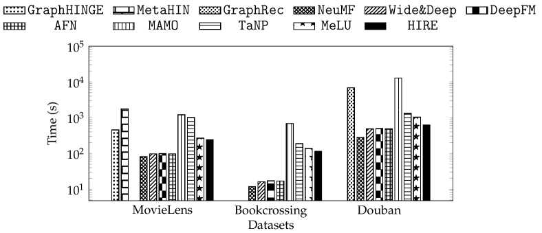
Figure 6: Total Test Time (second)

VI-C Efficiency

We compare the test time of HIRE with the baseline approaches, where the total test time for the 3 datasets on a single Tesla V100 GPU is presented in Fig. 6. Recall that the HIN-based approach GraphHINGE is only applicable for $\mathsf{MovieLens}$-$\mathsf{1M}$ and the social recommendation approach GraphRec is only applicable for $\mathsf{Douban}$. Here, we only compare for the user cold-start since the test time for the 3 cold-start scenarios is similar. The CF-based approaches, NeuMF, Wide&Deep, AFN and DeepFM are the most time-efficiency approaches, since they only take a pair of user and item with their potential features as input, and the model architectures are relatively simple. Our approach, HIRE, spends a longer time for prediction than the CF-based approaches due to the computational cost of multi-layer MHSA. However, the prediction of HIRE is faster than that of the other 6 approaches on average. The meta-learning approaches, MAMO, MetaHIN, TaNP and MeLU, leverage extra modules for model adaption. GraphHINGE needs to sample and model the neighborhood interactions from an HIN, which results in the second longest time in $\mathsf{MovieLens}$-$\mathsf{1M}$. GraphRec spends the second longest time for prediction since it deploys an additional Graph Neural Network to aggregate social relations. MAMO is significantly slower than HIRE, with about one order of magnitude. This is because MAMO is built upon the MAML algorithm and utilizes two specific memory modules, which have high time and space complexities. In a nutshell, HIRE outperforms other methods by achieving the best overall effectiveness while maintaining a competitive prediction efficiency.

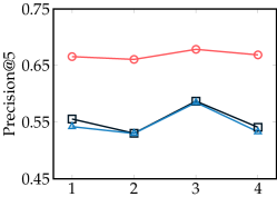
(a) # HIM Blocks

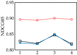
(b) # HIM Blocks

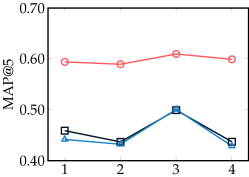
(c) # HIM Blocks

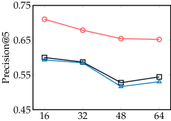
(d) # Users/Items

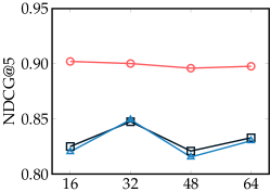
(e) # Users/Items

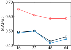
(f) # Users/Items

Figure 7: Sensitivity Analysis on $\mathsf{MovieLens}$-$\mathsf{1M}$

TABLE VI: Ablation Study for Different Attention Layers on $\mathsf{MovieLens}$-$\mathsf{1M}$

Blocks	User Cold-Start			Item Cold-Start			User & Item Cold-Start
	Pre.@5	NDCG@5	MAP@5	Pre.@5	NDCG@5	MAP@5	Pre.@5	NDCG@5	MAP@5
wo/ Item & Attribute	0.4465	0.7858	0.3232	0.4392	0.7600	0.3177	0.4663	0.7700	0.3440
wo/ User & Attribute	0.6552	0.8926	0.5838	0.5268	0.8174	0.4301	0.5227	0.8138	0.4239
wo/ User & Item	0.6752	0.8986	0.6040	0.5163	0.8128	0.4202	0.5067	0.8079	0.4073
wo/ User	0.6590	0.8925	0.5885	0.5272	0.8116	0.4223	0.5239	0.8111	0.4213
wo/ Item	0.4461	0.7866	0.3238	0.4414	0.7610	0.3193	0.4687	0.7700	0.3447
wo/ Attribute	0.4477	0.7865	0.3242	0.4413	0.7611	0.3200	0.4671	0.7699	0.3442
full model	0.6787	0.9002	0.6097	0.5871	0.8475	0.4993	0.5848	0.8493	0.5008

(a) Precision

(b) NDCG

(c) MAP

Figure 8: Impact of sampling methods on $\mathsf{MovieLens}$-$\mathsf{1M}$

VI-D Sensitivity Analysis

We investigate the parameter sensitivity of HIRE with respect to two key hyper-parameter configurations: (1) the number of the Heterogeneous Interaction Modules (HIM) in HIRE and (2) the number of users/items sampled in one prediction context. Due to space limitation, we present the evaluation results for the metrics at $k=5$ considering it can be regarded as a lower bound for all the metrics. First, we train HIRE model variants by varying the number of HIMs in $\{1,2,3,4\}$ on $\mathsf{MovieLens}$-$\mathsf{1M}$, where all the other hyper-parameters are fixed as default. Fig.  7(a), 7(b) and 7(c) show the test accuracy in the 3 cold-start scenarios. Here, HIRE with $3$ HIMs achieves the best performance, which is consistent to the different cold-start scenarios. As the number of HIMs increases, the model is able to capture increasingly high-order and complex interactions. However, more HIMs such as 4 will incur the risk of overfiting and lead to performance degradation in practice. In contrast, for $\mathsf{Bookcrossing}$ and $\mathsf{Douban}$, in our extra experiments, we observe that 2 and 4 HIM blocks achieve the best performance, respectively. Thereby, different datasets may need different configurations to reach the best result. Another observation is that HIRE in user cold-start is less sensitive to the number of HIMs, compared with item and user & item cold-start.

In addition, we also compare the accuracy of HIRE by varying the number of sampled users/items in the training and test context in $\{16,32,48,64\}$, where the results are shown in Fig. 7(d), 7(e) and 7(f). As the number of users/items increases, the performance of HIRE may not change monotonically. More users/items in the context matrices may provide richer information for the prediction, e.g., in the cases of 64 users/items, or bring noise information, e.g., in the cases of 48 users/items, which hurts the performance. For $\mathsf{MovieLens}$-$\mathsf{1M}$, setting the number of users/items to 32 yields the most impressive scores, whereas in our extra testing on $\mathsf{Bookcrossing}$ and $\mathsf{Douban}$, the setting of 64 yields the best scores. We speculate that the reason would be the latter two datasets have less attributes so that they need more users/items in the prediction context.

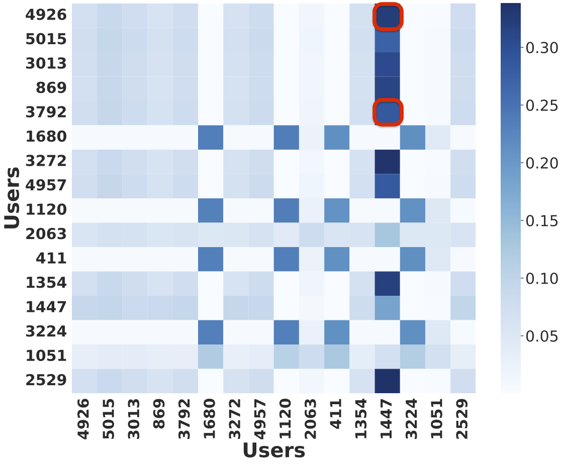
(a) Weights of MBU

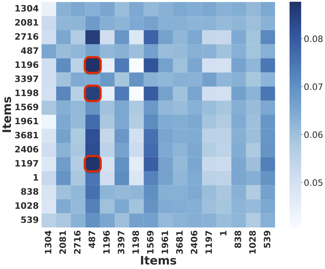
(b) Weights of MBI

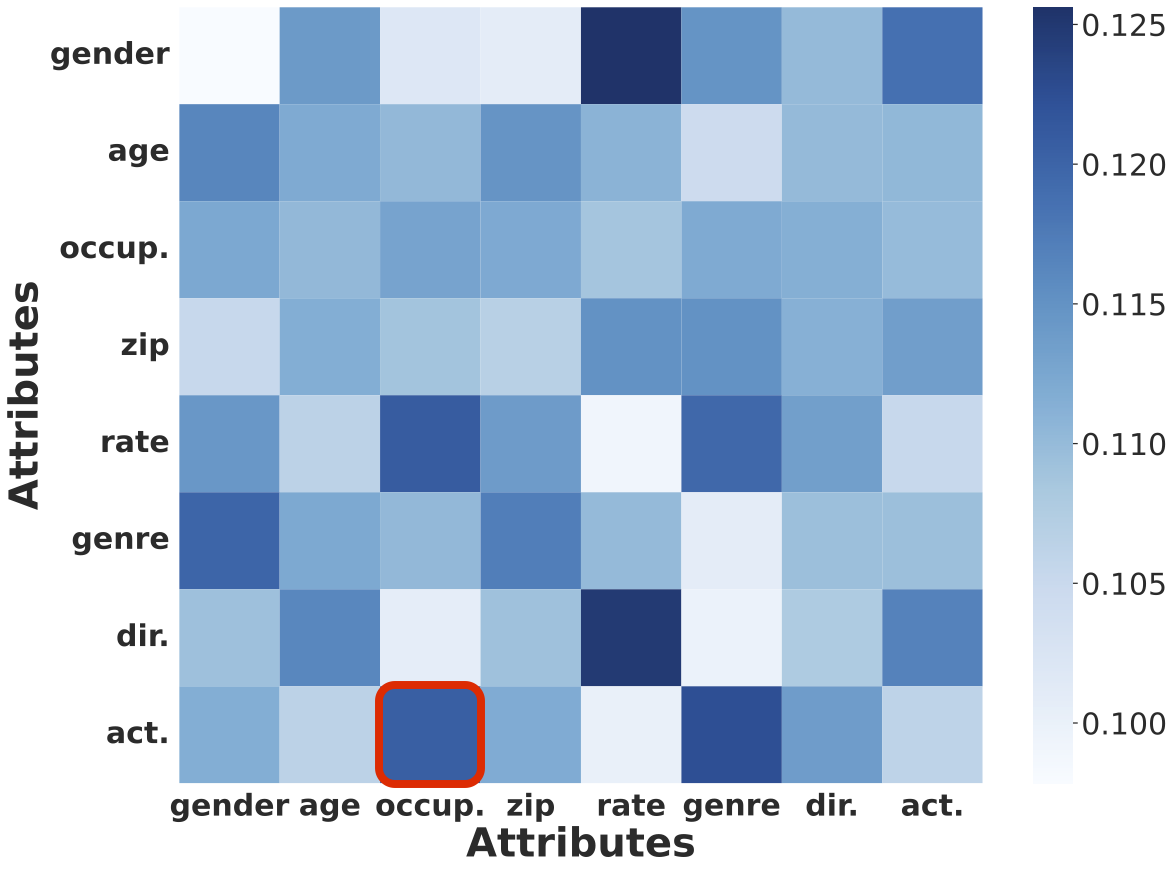
(c) Weights of MBA (high rating)

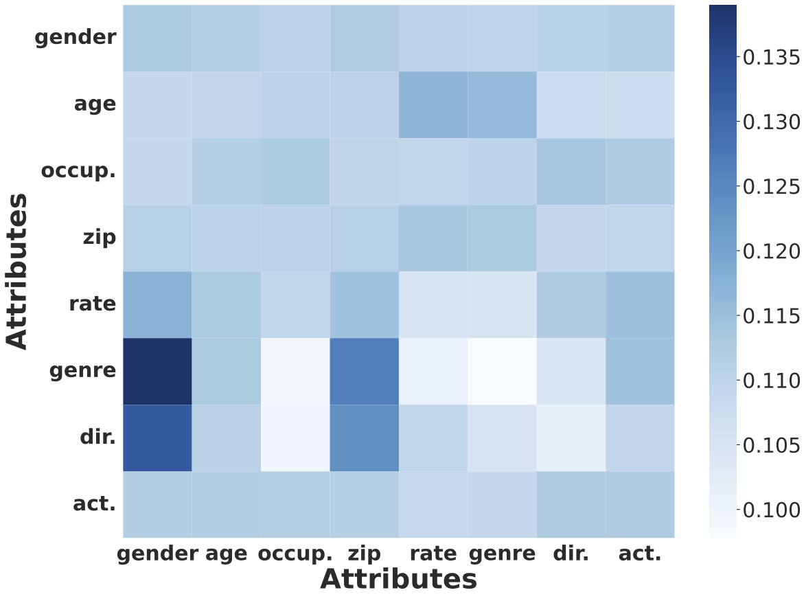
(d) Weights of MBA (low rating)

Figure 9: Visualizations of the Attention Weights in HIRE

VI-E Ablation Study

Impacts of the three types of attention layers. We conduct an ablation study to investigate the effectiveness of the 3 types of attention layers, attention between users, items and attributes, in HIRE. Here, we train 6 model variants on $\mathsf{MovieLens}$-$\mathsf{1M}$, where single types or combinations of two types of layers are removed for the model. Table VI lists the test performance of the model variants in 3 cold-start scenarios. The full model with the 3 types of attention layers achieves the overall best performance, indicating that the heterogeneous interactions from 3 different perspectives collaboratively contribute to the rating prediction. In addition, we find that the attention between items (or attributes) plays a more important role than attention between users in rating prediction, by comparing model variants wo/ Item (or wo/ Attribute) with model variant wo/ User. For $\mathsf{MovieLens}$-$\mathsf{1M}$, we speculate that the similarity between the movies and the similarity between the proprieties of users and movies influences the rating to a larger degree. Meanwhile, another possible reason would be the interactions between users may not be reliable. That is because there is a counter-intuitive observation on that the model variant wo/ Item (or wo/ Attribute) performs worse than the model variant wo/ User & Item (or wo/ User & Attribute). And the model with only attention between users, i.e., wo/ Item & Attribute, leaves the worst performance among all the model variants. The attention between users may learn irrelevant interactions, where deploying this layer alone or combining it with another single type of attention layer incurs extra noise for the prediction. Furthermore, in our experiments on $\mathsf{Bookcrossing}$ and $\mathsf{Douban}$ datasets, the full model consistently outperforms other variants.

Impacts of sampling methods. To study our neighborhood-based sampling strategy for context construction, we compare it with the random sampling strategy and feature similarity sampling strategy as an ablation. For the feature similarity sampling strategy, we compute the cosine similarity of attributes between target users (items) and other users (items). The users (items) with higher scores will be sampled. Fig. 8 shows the test result of HIRE on $\mathsf{MovieLens}$-$\mathsf{1M}$, by fixing the number of users and items as $32$. Here, our neighborhood-based sampling strategy is better than random sampling in all cases by $1.26\%$ on average. On the other two datasets, we also achieve similar results, further confirming the effectiveness of the neighborhood-based sampling strategy. The reason would be that compared with a fully randomized batch of users/items whose correlations are unknown, neighborhood-based sampling strategy is able to select more relevant neighbor users to construct the prediction context. That promotes HIRE to make more accurate predictions. Feature similarity sampling strategy tends to perform better than neighborhood-based in the user cold-start scenario. The reason would be that relevant users can be sampled via computing their feature similarity. For cold items, feature similarity is unable to select the most relevant items, which results in poor performance in other two scenarios.

VI-F Case Study

We conduct a case study to investigate whether HIM learns relevant and reliable interactions between users, items and attributes, and here we denote the three layers as MBU, MBI and MBA, respectively. We visualize the attention matrices for the prediction on $\mathsf{MovieLens}$-$\mathsf{1M}$ in Fig. 9. Here, the darker the cell, the higher the corresponding weight, and the stronger the implicit interaction learned by HIM. First, Fig. 9(a) shows the attention weights in MBU layer among 16 users for item $1,304$, which is an action and comedy movie, ’Butch Cassidy and the Sundance Kid’. In Fig. 9(a), as the highlighted red rectangle, user $1,447$ is deeply affected by user $4,926$ and $3,792$. We find that the three users share the same preference on item $1,304$. With the learned user interactions, HIRE predicts the ratings of the three users on item $1,304$ as $3.41$, $4.13$ and $4.20$, which is highly consistent to the ground-truth ratings, $3,4,4$, respectively. That indicates the interaction between users has a strong correlation to their ratings. Second, Fig. 9(b) shows the attention weights in MBI layer among 16 items for user $4,926$, who is a female student under 18 years old. Similarly, we observe that item $487$ is strongly affected by items $1,196$, $1,197$ and $1,198$. With the learned interaction between items, HIRE predicts the ratings of that user on item $487$ as $3.42$, and on items $1,196$, $1,197$ and $1,198$ as $3.88,3.95,3.86$, respectively. That is also consistent to the ground-truth ratings of $3$ for item $487$ and $4$ for the other three items. The results also demonstrate that the learned implicit interactions among items guide the model to predict similar ratings for interacted items. Finally, Fig. 9(c) and 9(d) present the attention weights among the 8 attributes in the MBA layer, for two user-item pairs, user 4,926 and item 1,304, user 1,051 and item 2,081, respectively. The former pair has a high rating of $4$. User $1051$ is a $18-24$ year old male technician/engineer and item $2081$ is a comedy ’Trees Lounge’. The user $1051$ gave a low rating $2$ to movie $2,081$. It is reasonable according to the occupation of user and genre of movie. As we can see, high rating pair has more attribute interactions. Actor attribute has interactions with occupation in Fig. 9(c). This means that the actor in the movie may be liked by people in a specific occupation. The latter one has less interactions between movie attributes and user attributes. It may because user has no interest to this movie. It is worth mentioning that the weight matrices are unsymmetrical due to the computation of attention (Eq. (2)), which indicates the interactions are single direction.

VII Conclusion

In this paper, we propose a fully data-driven recommender system HIRE that can model heterogeneous interactions for cold-start rating prediction. For target cold user/items, we adopt a neighborhood-based sampling strategy to sample prediction context from the user-item bipartite rating graph, and explore reliable interactions in the context. Specifically, we devise a Heterogeneous Interaction Module to jointly model the interactions in three levels, i.e., users, items and attributes, respectively. Comprehensive experiments on three real-world datasets validate the effectiveness of our model. HIRE outperforms CF-based approaches, social recommendation approaches, HIN-based approaches and state-of-the-art approaches with higher precision, NDCG and MAP by 0.22, 0.30 and 0.22 on average.

References

- [1] F. Lyu, X. Tang, H. Guo, R. Tang, X. He, R. Zhang, and X. Liu, “Memorize, factorize, or be naive: Learning optimal feature interaction methods for ctr prediction,” in 2022 IEEE 38th International Conference on Data Engineering (ICDE). IEEE, 2022, pp. 1450–1462.
- [2] W. Guo, C. Zhang, Z. He, J. Qin, H. Guo, B. Chen, R. Tang, X. He, and R. Zhang, “Miss: Multi-interest self-supervised learning framework for click-through rate prediction,” in 2022 IEEE 38th international conference on data engineering (ICDE). IEEE, 2022, pp. 727–740.
- [3] T. Qian, Y. Liang, Q. Li, and H. Xiong, “Attribute graph neural networks for strict cold start recommendation : Extended abstract,” in 39th IEEE International Conference on Data Engineering, ICDE 2023, Anaheim, CA, USA, April 3-7, 2023. IEEE, 2023, pp. 3783–3784.
- [4] H. Li, Y. Wang, Z. Lyu, and J. Shi, “Multi-task learning for recommendation over heterogeneous information network (extended abstract),” in 39th IEEE International Conference on Data Engineering, ICDE 2023, Anaheim, CA, USA, April 3-7, 2023. IEEE, 2023, pp. 3775–3776.
- [5] J. Cao, J. Sheng, X. Cong, T. Liu, and B. Wang, “Cross-domain recommendation to cold-start users via variational information bottleneck,” in 2022 IEEE 38th International Conference on Data Engineering (ICDE). IEEE, 2022, pp. 2209–2223.
- [6] G. Linden, B. Smith, and J. York, “Amazon. com recommendations: Item-to-item collaborative filtering,” IEEE Internet computing, vol. 7, no. 1, pp. 76–80, 2003.
- [7] S. Sedhain, A. K. Menon, S. Sanner, and L. Xie, “Autorec: Autoencoders meet collaborative filtering,” in Proceedings of the 24th international conference on World Wide Web, 2015, pp. 111–112.
- [8] X. He, L. Liao, H. Zhang, L. Nie, X. Hu, and T.-S. Chua, “Neural collaborative filtering,” in Proceedings of the 26th international conference on world wide web, 2017, pp. 173–182.
- [9] Y. Koren, R. Bell, and C. Volinsky, “Matrix factorization techniques for recommender systems,” Computer, vol. 42, no. 8, pp. 30–37, 2009.
- [10] S. Rendle, C. Freudenthaler, Z. Gantner, and L. Schmidt-Thieme, “Bpr: Bayesian personalized ranking from implicit feedback,” 2012.
- [11] B. Sarwar, G. Karypis, J. Konstan, and J. Riedl, “Item-based collaborative filtering recommendation algorithms,” in Proceedings of the 10th international conference on World Wide Web, 2001, pp. 285–295.
- [12] Y. Rong, X. Wen, and H. Cheng, “A monte carlo algorithm for cold start recommendation,” in Proceedings of the 23rd international conference on World wide web, 2014, pp. 327–336.
- [13] J. Tang, X. Hu, and H. Liu, “Social recommendation: a review,” Soc. Netw. Anal. Min., vol. 3, no. 4, pp. 1113–1133, 2013. [Online]. Available: https://doi.org/10.1007/s13278-013-0141-9
- [14] L. Wu, P. Sun, Y. Fu, R. Hong, X. Wang, and M. Wang, “A neural influence diffusion model for social recommendation,” in Proceedings of the 42nd international ACM SIGIR conference on research and development in information retrieval, 2019, pp. 235–244.
- [15] W. Fan, Y. Ma, Q. Li, Y. He, E. Zhao, J. Tang, and D. Yin, “Graph neural networks for social recommendation,” in The world wide web conference, 2019, pp. 417–426.
- [16] M. Jamali and M. Ester, “Trustwalker: a random walk model for combining trust-based and item-based recommendation,” in Proceedings of the 15th ACM SIGKDD international conference on Knowledge discovery and data mining, 2009, pp. 397–406.
- [17] J. Tang, X. Hu, H. Gao, and H. Liu, “Exploiting local and global social context for recommendation.” in IJCAI, vol. 13, 2013, pp. 2712–2718.
- [18] H. Ma, H. Yang, M. R. Lyu, and I. King, “Sorec: social recommendation using probabilistic matrix factorization,” in Proceedings of the 17th ACM conference on Information and knowledge management, 2008, pp. 931–940.
- [19] M. Jamali and M. Ester, “A matrix factorization technique with trust propagation for recommendation in social networks,” in Proceedings of the fourth ACM conference on Recommender systems, 2010, pp. 135–142.
- [20] J. Zhou, G. Cui, S. Hu, Z. Zhang, C. Yang, Z. Liu, L. Wang, C. Li, and M. Sun, “Graph neural networks: A review of methods and applications,” AI open, vol. 1, pp. 57–81, 2020.
- [21] J. Jin, J. Qin, Y. Fang, K. Du, W. Zhang, Y. Yu, Z. Zhang, and A. J. Smola, “An efficient neighborhood-based interaction model for recommendation on heterogeneous graph,” in Proceedings of the 26th ACM SIGKDD international conference on knowledge discovery & data mining, 2020, pp. 75–84.
- [22] X. Lin, J. Wu, C. Zhou, S. Pan, Y. Cao, and B. Wang, “Task-adaptive neural process for user cold-start recommendation,” in Proceedings of the Web Conference 2021, 2021, pp. 1306–1316.
- [23] H. Lee, J. Im, S. Jang, H. Cho, and S. Chung, “Melu: Meta-learned user preference estimator for cold-start recommendation,” in Proceedings of the 25th ACM SIGKDD International Conference on Knowledge Discovery & Data Mining, 2019, pp. 1073–1082.
- [24] M. Dong, F. Yuan, L. Yao, X. Xu, and L. Zhu, “Mamo: Memory-augmented meta-optimization for cold-start recommendation,” in Proceedings of the 26th ACM SIGKDD international conference on knowledge discovery & data mining, 2020, pp. 688–697.
- [25] H.-T. Cheng, L. Koc, J. Harmsen, T. Shaked, T. Chandra, H. Aradhye, G. Anderson, G. Corrado, W. Chai, M. Ispir et al., “Wide & deep learning for recommender systems,” in Proceedings of the 1st workshop on deep learning for recommender systems, 2016, pp. 7–10.
- [26] H. Guo, R. Tang, Y. Ye, Z. Li, and X. He, “Deepfm: a factorization-machine based neural network for ctr prediction,” arXiv preprint arXiv:1703.04247, 2017.
- [27] W. Cheng, Y. Shen, and L. Huang, “Adaptive factorization network: Learning adaptive-order feature interactions,” in Proceedings of the AAAI Conference on Artificial Intelligence, vol. 34, no. 04, 2020, pp. 3609–3616.
- [28] X. Yu, X. Ren, Y. Sun, B. Sturt, U. Khandelwal, Q. Gu, B. Norick, and J. Han, “Recommendation in heterogeneous information networks with implicit user feedback,” in Proceedings of the 7th ACM conference on Recommender systems, 2013, pp. 347–350.
- [29] H. Zhao, Q. Yao, J. Li, Y. Song, and D. L. Lee, “Meta-graph based recommendation fusion over heterogeneous information networks,” in Proceedings of the 23rd ACM SIGKDD International Conference on Knowledge Discovery and Data Mining, Halifax, NS, Canada, August 13 - 17, 2017. ACM, 2017, pp. 635–644.
- [30] C. Luo, W. Pang, Z. Wang, and C. Lin, “Hete-cf: Social-based collaborative filtering recommendation using heterogeneous relations,” in 2014 IEEE International Conference on Data Mining. IEEE, 2014, pp. 917–922.
- [31] Y. Sun, J. Han, X. Yan, P. S. Yu, and T. Wu, “Pathsim: Meta path-based top-k similarity search in heterogeneous information networks,” Proceedings of the VLDB Endowment, vol. 4, no. 11, pp. 992–1003, 2011.
- [32] E. Min, Y. Rong, T. Xu, Y. Bian, D. Luo, K. Lin, J. Huang, S. Ananiadou, and P. Zhao, “Neighbour interaction based click-through rate prediction via graph-masked transformer,” in Proceedings of the 45th International ACM SIGIR Conference on Research and Development in Information Retrieval, 2022, pp. 353–362.
- [33] Y. Lu, Y. Fang, and C. Shi, “Meta-learning on heterogeneous information networks for cold-start recommendation,” in Proceedings of the 26th ACM SIGKDD International Conference on Knowledge Discovery & Data Mining, 2020, pp. 1563–1573.
- [34] J. Snell, K. Swersky, and R. Zemel, “Prototypical networks for few-shot learning,” Advances in neural information processing systems, vol. 30, 2017.
- [35] S. Ravi and H. Larochelle, “Optimization as a model for few-shot learning,” in International conference on learning representations, 2016.
- [36] A. Graves, G. Wayne, and I. Danihelka, “Neural turing machines,” arXiv preprint arXiv:1410.5401, 2014.
- [37] C. Finn, P. Abbeel, and S. Levine, “Model-agnostic meta-learning for fast adaptation of deep networks,” in International conference on machine learning. PMLR, 2017, pp. 1126–1135.
- [38] M. Garnelo, J. Schwarz, D. Rosenbaum, F. Viola, D. J. Rezende, S. Eslami, and Y. W. Teh, “Neural processes,” arXiv preprint arXiv:1807.01622, 2018.
- [39] A. Vaswani, N. Shazeer, N. Parmar, J. Uszkoreit, L. Jones, A. N. Gomez, Ł. Kaiser, and I. Polosukhin, “Attention is all you need,” Advances in neural information processing systems, vol. 30, 2017.
- [40] J. Devlin, M.-W. Chang, K. Lee, and K. Toutanova, “Bert: Pre-training of deep bidirectional transformers for language understanding,” arXiv preprint arXiv:1810.04805, 2018.
- [41] T. Brown, B. Mann, N. Ryder, M. Subbiah, J. D. Kaplan, P. Dhariwal, A. Neelakantan, P. Shyam, G. Sastry, A. Askell et al., “Language models are few-shot learners,” Advances in neural information processing systems, vol. 33, pp. 1877–1901, 2020.
- [42] A. Dosovitskiy, L. Beyer, A. Kolesnikov, D. Weissenborn, X. Zhai, T. Unterthiner, M. Dehghani, M. Minderer, G. Heigold, S. Gelly et al., “An image is worth 16x16 words: Transformers for image recognition at scale,” arXiv preprint arXiv:2010.11929, 2020.
- [43] R. Ying, R. He, K. Chen, P. Eksombatchai, W. L. Hamilton, and J. Leskovec, “Graph convolutional neural networks for web-scale recommender systems,” in Proceedings of the 24th ACM SIGKDD International Conference on Knowledge Discovery & Data Mining, KDD 2018, London, UK, August 19-23, 2018, Y. Guo and F. Farooq, Eds. ACM, 2018, pp. 974–983.
- [44] M. Zhang and Y. Chen, “Inductive matrix completion based on graph neural networks,” in 8th International Conference on Learning Representations, ICLR 2020, Addis Ababa, Ethiopia, April 26-30, 2020. OpenReview.net, 2020.
- [45] E. Min, R. Chen, Y. Bian, T. Xu, K. Zhao, W. Huang, P. Zhao, J. Huang, S. Ananiadou, and Y. Rong, “Transformer for graphs: An overview from architecture perspective,” CoRR, vol. abs/2202.08455, 2022.
- [46] F. M. Harper and J. A. Konstan, “The movielens datasets: History and context,” Acm transactions on interactive intelligent systems (tiis), vol. 5, no. 4, pp. 1–19, 2015.
- [47] E. Zhong, W. Fan, J. Wang, L. Xiao, and Y. Li, “Comsoc: Adaptive transfer of user behaviors over composite social network,” in Proceedings of the 18th ACM SIGKDD International Conference on Knowledge Discovery and Data Mining, ser. KDD ’12. New York, NY, USA: ACM, 2012.
- [48] E. Zhong, W. Fan, and Q. Yang, “User behavior learning and transfer in composite social networks,” ACM Trans. Knowl. Discov. Data, vol. 8, no. 1, pp. 6:1–6:32, Feb. 2014.
- [49] C.-N. Ziegler, S. M. McNee, J. A. Konstan, and G. Lausen, “Improving recommendation lists through topic diversification,” in Proceedings of the 14th international conference on World Wide Web, 2005, pp. 22–32.
- [50] Y. You, J. Li, S. Reddi, J. Hseu, S. Kumar, S. Bhojanapalli, X. Song, J. Demmel, K. Keutzer, and C.-J. Hsieh, “Large batch optimization for deep learning: Training bert in 76 minutes,” 2019.
- [51] M. Zhang, J. Lucas, J. Ba, and G. E. Hinton, “Lookahead optimizer: k steps forward, 1 step back,” vol. 32, 2019.
- [52] “Pytorch,” https://github.com/pytorch/pytorch.
- [53] K. Järvelin and J. Kekäläinen, “Cumulated gain-based evaluation of ir techniques,” ACM Transactions on Information Systems (TOIS), vol. 20, no. 4, pp. 422–446, 2002.