The inclusive Synthetic Control Method
Abstract
We introduce the inclusive synthetic control method (iSCM), a modification of synthetic control type methods that allows the inclusion of units potentially affected directly or indirectly by an intervention in the donor pool. This method is well suited for applications with either multiple treated units or in which some of the units in the donor pool might be affected by spillover effects. Our iSCM is very easy to implement using most synthetic control type estimators. As an illustrative empirical example, we re-estimate the causal effect of German reunification on GDP per capita allowing for spillover effects from West Germany to Austria.
Keywords: Synthetic Control Method, spillover effects, causal inference.
JEL classification: C21, C23, C31, C33.
1 Introduction
The synthetic control method (SCM) introduced by Abadie and Gardeazabal (2003) and further developed in Abadie et al. (2010) and Abadie et al. (2015) allows the estimation of the causal effect of a policy intervention in settings where only a few treated and control units are observed over a long time period. The idea behind this method is to create a linear combination of control units that mimic what would have happened to the treated units in the absence of the intervention. The weights given to each control unit are chosen to minimize the distance in the pre-intervention characteristics of the treated and the synthetic control units. The causal effect of the intervention is then estimated as the difference between the observed outcome of the treated and that of the synthetic control in the post-intervention period. One of the key assumptions of the SCM is that only units that are not affected by the interventions are included in the control group, often referred to as the donor pool. This might be problematic in at least two scenarios: i) some of the treated units would ideally be included in the donor pool to improve the pre-intervention fit; ii) some of the control units are affected by the intervention indirectly but excluding them from the donor pool deteriorates the pre-intervention fit substantially. As a motivating example, consider the German reunification study by Abadie et al. (2015) (see also Abadie (2021)). The authors point out it is possible that German reunification had spillover effects on neighboring countries such as Austria. As Austria receives a high weight (42%), such a spillover effect, if large, would introduce a large bias. Given that Austria plays an important role in constructing “synthetic West Germany” excluding it from the donor pool is likely to reduce the quality of the match between treated and synthetic units.
Our main contribution is to introduce the inclusive synthetic control method (iSCM), a novel procedure that allows us to eliminate post-intervention effects from control units and safely include them in the donor pool. We exploit the fact that the synthetic control weights are estimated only using pre-intervention data and no unit is treated in this period. Thus, when “potentially affected” units are added to the donor pool, the synthetic control unit becomes a weighted average of the outcomes of all the units in the donor pool and the effects of the intervention on “potentially affected” units, each weighted by their synthetic weights. This implies that comparing the “main treated” and its synthetic control version gives an estimate of the true effect minus the effects on other units, each weighted by their synthetic weights. If we create a synthetic control version of all “potentially affected” units (including the “main treated” unit in the respective donor pools) we can get an estimate of the true effects on those units plus the effects on other affected units (including the “main treated”), each weighted by their synthetic weights. This process yields a system of equations with “m” unknowns, comprising the treatment effect on the “main treated” unit and the “m-1” effects on “potentially affected” units which can be easily solved using Cramer’s rule. This means that our procedure does not require any modification of the synthetic control estimator, and any alternative SC-type method which creates a synthetic control unit as a weighted average of the outcome of the units in the donor pool can be used instead (see, for example, Abadie and L’Hour 2021, Amjad et al. 2018, Ben-Michael et al. 2021, Ben-Michael et al. 2022, Doudchenko and Imbens 2017, Ferman and Pinto 2021, Kellogg et al. 2021, Xu 2017). In addition to the assumptions behind the particular SC-estimator chosen, our iSCM requires prior knowledge on which units can be “potentially affected” by the treatment. Although iSCM only requires the existence of at least one “pure control” unit receiving non-zero weight, our method becomes less reliable as the number of “potentially affected” units increases. Thus, it is advisable to impose assumptions that limit this number. This is in line with the literature on spillover effects, in which it is often assumed that interactions between units are only possible if they belong to a certain group, but no interactions are allowed between different groups (Cerqua and Pellegrini 2017, Forastiere et al. 2021, Huber and Steinmayr 2019, Vazquez-Bare 2022). This is also the case for the few extensions of the synthetic control method that allow for the presence of spillover effects. Grossi et al. (2020) propose reducing the donor pool to only units not affected by spillovers. They estimate the effects for the treated unit using a SCM with the restricted donor pool and the spillover effects by comparing units affected by spillover and the restricted donor pool. Their method is very effective in applications in which the restricted donor pool is sufficient to construct a “good” synthetic control. However, in a setting where including units affected by spillover in the donor pool improves the pre-intervention fit, as in the German reunification example, their method would likely produce less reliable results. Cao and Dowd (2019) provide a different identification and estimation strategy focusing more on the spillover effects structure. In contrast, our approach can also be used in applications where one wants to include treated units in the donor pool. Another difference between the two approaches is that we allow for using any SC-type estimator as soon as the final estimator is based on a weighted average of the outcome of the units in the donor pool. Although our paper is related to the literature on spillover effects, our results also apply when there are multiple treated units and no spillover effects. Moreover, our identification relies on being able to observe the potential outcome under non-treatment of every unit in the pre-intervention period and it differs from the identification results in the spillover/peer effect literature.
We provide a data-driven approach to check whether excluding “potentially affected” units from the donor pool can potentially lead to a large bias. Even in applications where the expected bias is small we still recommend using iSCM as a robustness check especially if the “potentially affected” units receive a high weight.
The rest of the paper is organized as follows: Sections 2 describe the iSCM; Section 3 discuss the special case where there is only one “potentially affected” unit; Section 4 compare the estimation errors of SCM and iSCM; in Section 5 we compare iSCM and a “restricted” SCM and propose an implementation procedure; Section 6 suggests possible inference procedures; Section 7 shows the results of the empirical application; and Section 8 concludes the paper.
2 The inclusive synthetic control method
Assume we observe units for periods. For each unit at time we observe the outcome of interest and a set of predictors of the outcome , which often includes pre-intervention values of . We refer to the treated unit (unit ) as the “main treated”. We also assume that the units in the donor pool, include units (units to ) that are directly or indirectly affected by the intervention (“potentially affected” hereafter), i.e., they are either other treated units that we would like to include in the donor pool or control units that might be affected by spillover effects from the main treated. We refer to units through , as “pure control” units and assume that they are not affected by the intervention at all. We define the potential outcome as the outcome that the “main treated” unit would obtain under the intervention at time . We define the potential outcome of “potentially affected” units at time as , which represents either the outcome of a unit “potentially affected” by spillover effects or simply the potential outcome under treatment if unit is a different treated unit. Finally, we define as the potential outcome in the absence of the intervention. We assume that there are no anticipation effects together with the standard stable unit treatment value assumption (SUTVA) with the exception of the potential presence of spillover effects on units, who are chosen a priori. This assumption can be formalized as Assumption 1:
-
•
In the pre-intervention period, = for all units.
-
•
In the post-intervention period, = for the “pure control”.
-
•
In the post-intervention period, = for the “main treated”.
-
•
In the post-intervention period, = for the “potentially affected units” .
Assumption 1 may be restrictive in scenarios where it is unclear which units might be “potentially affected” by spillover effects. However, it is standard in contexts where the “potentially affected” units are other treated units. We are interested in the causal effect of the intervention on the “main treated” at time , denoted by , and the causal effects on the other “potentially affected” units denoted by , defined as
and
To identify these causal effects, we need to recover and for in the post-intervention period.
Assume we use a SC-type estimator , which estimates as a weighted average of the post-intervention outcomes of the units in the donor pool, e.g., the original SCM as described in Abadie et al. (2010). Let the vector of weights be the estimated weights of the chosen SC-type estimator that includes also the “potentially affected” units in the donor pool, under Assumption 1, we have
Therefore, under Assumption 1, we can decompose the estimation error333We will refer to the estimation error as bias hereafter. of , in two parts:
| (1) |
Similarly, consider a generic “potentially affected” unit , . Let the vector of weights estimated to create a SC-type estimator of that includes the “main treated” (unit 1), the other “potentially affected” units, as well as the “pure” control units in the donor pool. Assumption 1 implies that, , we have
Therefore under Assumption 1 we can decompose the estimation error of , in two parts:
| (2) |
Looking at the bias decomposition in (1) and (2) it is clear that we have two distinct sources of bias. The first, , relates to how well the chosen SC-type estimators approximate the post-intervention counterfactual. This is the usual source of bias we encounter when using any SC-type estimator. The second, , is induced by the fact that we are using units that are “potentially affected” by the intervention in the donor pull. This type of bias solely depends on whether or not a given (“potentially affected”) unit receives weight and its respective treatment effect but not on how “good” the chosen estimator is in recovering .
We will now assume that we have chosen a SC-type estimator to recover for which the first source of bias is negligible, formally
Assumption 2: The SC-type used to estimate satisfy .
We state Assumption 2 in terms of estimated weights without any loss of generality and simplify the discussion. Alternatively we can assume that the set of weights converges to a set of weights such that . When using the original SC-estimator, Assumption 2 amounts to assuming an (approximately) perfect fit444see the discussion in Abadie (2021), Ferman and Pinto (2021), and Powell (2018) about the lack of a perfect fit.. We state assumption 2 in very general terms as our results apply to any SC-type estimator that can be written as a weighted average of the control units post-intervention outcomes. For example, for the original SCM one can use the results in Zhang et al. (2022), and state Assumption 2 accordingly. Depending on the chosen estimator, one can state Assumption 2 more precisely. A non-exhaustive list of possible estimators includes the one proposed in: Abadie and L’Hour 2021, Amjad et al. 2018, Ben-Michael et al. 2021, Ben-Michael et al. 2022, Doudchenko and Imbens 2017, Ferman and Pinto 2021, Kellogg et al. 2021, Xu 2017.
Lemma 1:
Under Assumption 1 and 2
Proof of Lemma 1:
Under Assumption 1, we have
Thus Assumption 2 immediately implies
Remark 1:
It is important to notice that for each unit , if either or is zero, that unit does not induce any extra bias in . This implies that units that receive a low estimated weight need to have an extremely large effect to induce a non-negligible bias in . For this reason, units that receive a low weight can be relatively safely treated as “pure controls” when estimating in empirical applications.
Remark 2:
When using SC-type estimators that allow for negative weights one needs to check the magnitude of the weights given to “potentially affected” units. For estimators that use a bias correction, one needs to subtract the estimated bias from the outcome of all units before running our iSCM (see equation (16) in Abadie 2021).
In addition to Assumption 2, we assume that, , we have chosen a SC-type estimator to recover for which the bias is negligible, formally
Assumption 3: The SC-estimator chosen to estimate satisfy
Lemma 2:
Under Assumption 1 and 3
| (3) |
Proof of Lemma 2:
Under Assumption 1 we have
| (4) |
with . Under assumption 3 it follows that
Combining the results of Lemma 1 and Lemma 2, and ignoring the estimation biases , without loss of generality, the following system of equations holds
After some simple manipulations, we obtain555One can add the biases , on the left-hand side of each equation, however, they are negligible under assumptions 2 and 3. We show how these biases impact our iSCM estimator in the special case with in Section 4 below. :
This is a system of equations with unknowns, i.e., the treatment effect on the “main treated” and the effects on the “potentially affected” units.
We can write this system in matrix form, denoted by the () vector of unknown quantities (our effects of interest), by the () matrix of known quantities (our estimated weights) that has 1 on the main diagonal and by the () vector of known quantities (biased estimated effects), as
| (5) |
We now assume that is invertible, namely
Assumption 4: is non-singular.
It is easy to show that is always invertible, if , except for the extreme cases in which two units give weight 1 to each other and/or every single weight associated with the “pure control” units is zero (see Appendix A.1).
We now state our main result in the following theorem.
Theorem 1:
Under Assumptions 1, 2, 3, and 4, we have
Proof of Theorem 1:
The result immediately follows from lemma 1 and 2 and using the fact that under Assumption 4 is invertible.
The result in Theorem 1 can be readily used to identify our effects of interest by simply applying Cramer’s rule:
where is the matrix obtained by replacing the -th column of by the vector .
The expression above makes it very easy to construct estimators for our causal effects of interest that only require very basic linear algebra operations together with the preferred SC-type estimator for the weight matrix and the vector .
3 An example with a single “potentially affected” unit
To further illustrate our results, it is useful to consider the special case in which, together with the “main treated” unit, only one additional unit is “potentially affected” by the intervention (). First, we show the standard case and then the simplified case in which including the “main treated” in the donor pool of the “potentially affected” unit is not necessary.
With only one “potentially affected” unit, the system of equation defined in Section 2, again ignoring the estimation errors, simplifies to
where () is the estimated effect for the “main treated”; () is the estimated effect for the “potentially affected” unit; () and () are the estimated weights; () and () are the unknown effects.
Therefore, we have
To derive expressions for our estimators, we need to find , , and , which are given by
Following Cramer’s rule, we obtain
| (6) |
In this case, it is easy to see that is always different from zero, except when = . Thus, our effects of interest are always identified unless the “main treated” gives weight 1 to the other “potentially affected” unit, which in turn gives weight 1 to the “main treated”. This would be the case, for example, if there are no “pure control” units.
An interesting special case is when we do not need to include the “main treated” in the donor pool of the “potentially affected” unit. In this case, the system of equations further simplifies to
| (7) | ||||
| (8) |
Thus, estimating and becomes substantially easier.
4 Bias comparison between iSCM and SCM for
So far we have ignored the estimation biases . When ,
We can derive the bias of by adding those biases into equation (6)
The bias of approaches zero as the estimation biases and approach zero. In contrast, if we include “potentially affected” units, , even when approaches zero.
Note that is proportional to by a factor of . To compare the two biases, we can express as and compare each term with the one of the bias of which is . Clearly, the first term of , , is larger in magnitude than the first term of , . We can easily determine the exact difference by calculating . For example, in our application where and , . Thus, is about 16% larger in magnitude than . However, the second terms of the biases of and are driven by and , respectively. Note that, represents the estimation error in estimating . Therefore, unless the chosen SC-type estimator of performs poorly, will be significantly smaller in magnitude than , implying that is generally much smaller than .
In case it is not necessary to include the “main treated” in the donor pool of the “potentially affected” unit, we have
Thus, as soon as we have chosen a SC-type estimator such that its bias () is smaller in magnitude than its target parameter (), will always be smaller than .
5 iSCM vs “restricted” SCM
When using SC-type estimators, it is advisable to include in the donor pool units with similar characteristics and those possibly affected by similar shocks as the treated unit. Often, these units are either directly or indirectly affected by the intervention. For instance, it is likely that other treated units or units “potentially affected” by spillover effects are the closest (geographically and/or economically) to the “main treated” unit. For example, Abadie (2021) proposes including units “potentially affected” by spillover in the donor pool, even if they induce a bias.
Indeed, discarding “potentially affected” units could substantially decrease the match quality between the characteristics of the treated and the synthetic control, as those units are typically the closest to the treated. Therefore, choosing between our iSCM and a “restricted” version of SCM, where “potentially affected” units are excluded, depends on the importance of the excluded units in creating the synthetic control.
In the Appendix’s Section A.2, we demonstrate that iSCM may be superior to a “restricted” SCM even in scenarios where both “main treated” and “potentially affected” units are within the “pure control” units’ convex hull. In this scenario, a “restricted” SCM will potentially work, however, if the “potentially affected” units are the closest to the “main treated”, excluding them might increase interpolation bias. Additionally, we explore cases more common in empirical settings, where either or both the “main treated” and “potentially affected” units fall outside the convex hull.
To understand whether we expect a large bias by excluding “potentially affected” units, before implementing our iSCM, we advise taking the following steps to assess the potential gains of using our method instead of running a “restricted” SCM. When the SC-type estimator used is the one proposed by Abadie et al. (2010), we suggest following the procedure described below before adopting our method.
-
1.
Implement SCM, including units “potentially affected” by the intervention (i.e., other treated units or units affected by spillovers).
-
•
If all “potentially affected” units receive low or zero weights, they induce a negligible bias and can be used as “pure controls” in a SCM.
-
•
If some of the “potentially affected” units receive high weights, proceed with step 2.
-
2.
Implement the “restricted” SCM, i.e., excluding units “potentially affected” by the intervention and:
-
(a)
Compare the bias in terms of predictors () between the “restricted” SCM and the “unrestricted” SCM;
-
(b)
Compare Root Mean Squared Prediction Errors (RMSPEs) in the pre-intervention period of the “restricted” SCM and “unrestricted” SCM.
-
(a)
-
•
If () and , we advise using the “restricted” SCM as main specification and iSCM as a robustness check666Alternatively, one could divide the pre-intervention period into a training period and a validation period, estimate the two models during the training period, and compare their RMSPEs in the validation period. Note that the “restricted” SCM does not have by construction an RMSPE that is greater than or equal to that of the “unrestricted” one, see for example Section 7..
-
•
If () and/or , we advise using our iSCM.
Repeat these steps for each “potentially affected” unit as if it were the “main treated”. A similar procedure can be used for other SC-type estimators. In case there is no substantial gain from including the treated in the donor pool of “potentially affected” units, our iSCM becomes easier to implement, as shown in Equation 7. Finally, it’s worth comparing the results of the three methods, keeping in mind that the “unrestricted” SCM is biased if any of the units in the donor pool receiving non-negligible weight is affected by the treatment.
6 Inference
Dealing with only a small number of units makes inference for synthetic control-based methods like ours complicated. We can, however, easily adapt existing methods to our setting. The most popular choice is to implement permutation tests. Abadie et al. (2010) and Abadie et al. (2015) propose placebo tests in time, i.e., reassigning the intervention artificially before its real implementation, and placebo tests in-space, i.e., reassigning the intervention artificially for units in the control group. The latter approach is often preferred because of possible shocks that might have occurred in the past that affect units differently. Placebo tests in space measure the statistical significance of the effect through the ratio between the RMSPE in the post-treatment period and in the pre-treatment period.
To run the in-space placebo test for , all we need to do is subtract the estimated effects from the outcomes of “potentially affected” units. That is, we replace with , for all , and . Similarly, to construct a placebo test for for a generic “potentially affected” unit , we need to subtract the estimated effects from the outcomes of all other “potentially affected” units as well as the “main” treated unit, leaving the outcome of unit untouched.
This idea can easily be applied to other inference procedures available in the literature (see, e.g., Cao and Dowd 2019; Chernozhukov et al. 2021; Firpo and Possebom 2018; Gobillon and Magnac 2016; Li 2019). For example, the inference procedure of Chernozhukov et al. (2021) can be easily adapted to our framework by taking into account that the post-intervention observed outcome of each “potentially affected” unit includes its treatment effect. This has to be considered both in the first step, i.e., in the construction of the data under the null hypothesis and in the second step to compute the SCM residuals.
7 Empirical example
In this section, we use iSCM to estimate the effect of German reunification on West Germany’s GDP per capita. In October 1990, less than a year after the fall of the Berlin wall in November 1989, the German Democratic Republic (“East Germany”) and the Federal Republic of Germany (“West Germany”) were officially reunified. German reunification, defined as one of the most important historical milestones of European history after 1945, most likely affecting not only the German economy but also the economies of other European countries.
As discussed in Abadie et al. (2015) and Abadie and L’Hour (2021), German reunification could have had negative spillover effects on Austria’s economic growth because West Germany diverted demand and investment from Austria to East Germany. Austria has historically had tight links with Germany: the two countries share the same language and, to a great extent, a common history. In 1938, Austria was annexed by the Third Reich, which benefited from Austria’s raw materials and labor to complete German rearmament. In 1945, Austria was separated from Germany. However, the economic cooperation between Austria and West Germany continued during the Cold War. Given these strong cultural and economic ties, it is arguably important to include Austria in the donor pool when constructing a synthetic version of West Germany. Therefore, our iSCM is very well suited for estimating the impact of the German reunification not only on West Germany but also on Austria.777Given that other European countries receive very little weight, the impact of potential spillover effects on those countries would likely be negligible, as shown in Lemma 1. Results for the case in which Switzerland and the Netherlands are considered as “potentially affected” units are available from the authors upon request.
We use the same country-level panel data of Abadie et al. (2015). The data cover the period 1960-2003, with the post-intervention period starting in 1990. In addition to Austria, the remaining “pure control” countries in the donor pool include 15 other OECD countries: Australia, Belgium, Denmark, France, Greece, Italy, Japan, the Netherlands, New Zealand, Norway, Portugal, Spain, Switzerland, the United Kingdom, and the United States. The outcome variable is real GDP at Purchasing Power Parity (PPP) per capita measured in 2002 USD.
We start by implementing the procedure described in Section 5. First, we replicate the SCM estimate of Abadie et al. (2015) and check the weight assigned to Austria888We refer to Abadie et al. (2015) for a detailed discussion of the estimation procedure.. Given that Austria does receive the highest weight (42%) we can proceed to step 2, i.e., implementing the “restricted” SCM, i.e., excluding Austria from the donor pool, keeping the same specification and estimation procedure used for the “unrestricted” SCM.
Table 1 suggests that the “unrestricted” synthetic version of West Germany (second column) is much closer in therms of observable characteristics to West Germany (first column) than the “restricted” version (third column).
Next, we compare the pre-intervention RMSPEs of the “unrestricted” and “restricted” SCM. The RMSPE of the latter (270.74) is larger than the one of the former (119.07). Therefore, we expect iSCM to perform better than “restricted” SCM. We now repeat the same procedure to decide whether West Germany should be included in synthetic Austria’s donor pool. First, we check whether West Germany receives a non-negligible weight. To construct synthetic Austria, we must use a slightly different specification than the one used for creating synthetic West Germany. In particular we are not able to chose the weights assigned to the predictors using the sample splitting methods described in Abadie et al. (2015). As described in Gehler and Graf (2018), in 1980, not long before the sample split cut-off, Austria provided several loans to East Germany, and in return, Austrian nationalized industries received large-scale orders. This most likely stimulated Austria’s exports and contributed to job creation in its industries. Thus, the sample split procedure might catch the effect of this economic shock. This is corroborated by the fact that using this method to chose the predictor weights leads to a poor pre-intervention fit. For this reason, we decided to follow the data driven procedure suggested by Abadie et al. (2010) instead.
As shown in Table 2, Synthetic Austria gives the highest weight to West Germany. Thus, we can proceed to step 2, i.e., checking how well “restricted” (excluding West Germany) and “unrestricted” synthetic Astria matches real Austria’s observable characteristics and comparing the pre-intervention RMPEs of the two specifications.
Table 1 suggests that the “unrestricted” synthetic Austria (second column) does a better job of reproducing Austria’s (first column) pre-reunification predictors than the “restricted” version (third column), except for GDP per capita. The pre-intervention RMSPE of the “restricted” SCM (181.22) is slightly lower than the one of the “unrestricted” version (194.67). However, the difference is rather small. Taking everything into account, we argue that it is better to include West Germany in Austria’s donor pool.
| Unrestricted | Restricted | Unrestricted | Restricted | ||
|---|---|---|---|---|---|
| West Germany | Observed | synthetic | synthetic | Bias | Bias |
| GDP per capita | 15,808.90 | 15,804.64 | 16,138.83 | 4.26 | 329.93 |
| Trade openness | 56.78 | 56.91 | 50.73 | 0.14 | 6.04 |
| Inflation rate | 2.60 | 3.51 | 3.38 | 0.91 | 0.79 |
| Industry share | 34.54 | 34.38 | 33.30 | 0.15 | 1.24 |
| Schooling | 55.50 | 55.23 | 50.71 | 0.27 | 4.79 |
| Investment rate | 27.02 | 27.04 | 25.70 | 0.02 | 1.31 |
| Unrestricted | Restricted | Unrestricted | Restricted | ||
| Austria | Observed | synthetic | synthetic | Bias | Bias |
| GDP per capita | 10781.80 | 10798.41 | 10778.61 | 16.61 | 3.19 |
| Trade openness | 69.45 | 69.43 | 83.13 | 0.02 | 13.68 |
| Inflation rate | 4.91 | 4.92 | 5.59 | 0.01 | 0.68 |
| Industry share | 37.81 | 37.81 | 37.58 | 0.00 | 0.23 |
| Schooling | 53.25 | 45.71 | 35.44 | 7.54 | 17.81 |
| Investment rate | 26.64 | 26.64 | 27.03 | 0.00 | 0.38 |
| West Germany | Austria | |||
| Country | Unrestricted | Restricted | Unrestricted | Restricted |
| West Germany | - | - | 0.33 | - |
| Austria | 0.42 | - | - | - |
| Australia | 0 | 0 | 0 | 0 |
| Belgium | 0 | 0 | 0.12 | 0.511 |
| Denmark | 0 | 0 | 0 | 0 |
| France | 0 | 0 | 0 | 0 |
| Greece | 0 | 0 | 0 | 0 |
| Italy | 0 | 0 | 0 | 0 |
| Japan | 0.16 | 0.216 | 0.21 | 0.31 |
| Netherlands | 0.09 | 0.3 | 0.31 | 0.06 |
| New Zealand | 0 | 0 | 0 | 0 |
| Norway | 0 | 0 | 0.03 | 0 |
| Portugal | 0 | 0 | 0 | 0 |
| Spain | 0 | 0 | 0 | 0 |
| Switzerland | 0.11 | 0.089 | 0 | 0.12 |
| UK | 0 | 0 | 0 | 0 |
| USA | 0.22 | 0.395 | 0 | 0 |
Now we can use the “unrestricted” SCM estimates of , , the weight assigned to Austria , and the weight assigned to West Germany to estimate , and as
We can also construct the matrix , and check whether it is non-singular as required by Assumption 4. Given the estimated weights we get
As , Assumption 4 holds in this application, and we can safely use our iSCM estimators.
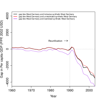
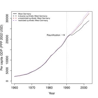
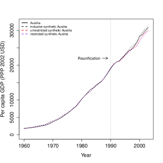
Figure 1 shows our main results. In Panel 1a and 1b we report the gaps estimated by the “unrestricted” SCM, the “restricted” SCM, and our iSCM, for West Germany and Austria, respectively999Notice that the “unrestricted” SCM and the iSCM are identical in the pre-treatment period because the spillover effect due to German reunification only happens after the intervention.. In Panel 1c we plot the GDP per capita trajectories (1960–2003) of Real West Germany, its “unrestricted” synthetic version, its “restricted” synthetic version, and its inclusive synthetic version. Panel 1d produces an analogous plot for Austria.
For West Germany, we can observe that both the standard and the inclusive synthetic version of West Germany in the pre-reunification period almost perfectly reproduce West Germany’s per capita GDP. Meanwhile, excluding Austria substantially worsens the pre-reunification fit. This confirms the importance of including Austria in the donor pool. Abadie et al. (2015) find a negative effect of the reunification on West Germany’s per capita GDP, which was reduced by approximately 7.67% per year on average relative to the 1990 baseline level. Our iSCM results are not very different from those of Abadie et al. (2015) and confirm their expectation about the potential direction of the bias, implying an even more negative effect of reunification. However, the difference between the trends in per capita GDP between iSCM and SCM is generally small: our iSCM estimate implies a negative effect that is up to 1.50% larger than the one estimated with a standard SCM.
If we look at the estimated spillover effects for Austria we draw similar conclusions. In the post-reunification period, iSCM estimates a decrease in per capita GDP of only up to 708 USD. However, this effect is unlikely to be statistically significant (see Figure Panel ). It is important to notice that both the “unrestricted” SCM and the “restricted” SCM estimate a positive spillover effect for Austria, up to 894 and 1350 USD, respectively. However, we know a priori that the “unrestricted” SCM is biased and its bias is . Given we have strong evidence that is negative, we do expect the “unrestricted” SCM to overestimate . Thus, the fact that both the “unrestricted” and the “restricted” SCM estimate positive spillover effects underscores the necessity of including West Germany in the donor pool and employing our iSCM in this application.
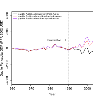
Finally, Panels 2a and 2b show the ratios between the RMSPEs in the post- and pre-reunification of West Germany’s donor pool and Austria’s donor pool, respectively. We can observe that West Germany’s value is very high and is the largest compared to any other countries in the donor pool. On the other hand, Austria’s RMSPE ratio is the second lowest indicating the spillover effect is not significant, as we mentioned above.


8 Conclusion
We introduce iSCM, a modification of the SCM that allows the inclusion of units “potentially affected” by an intervention in the donor pool. Our method is useful in applications where it is either important to include other treated units in the donor pool or where some of the units in the donor pool are affected indirectly by the intervention (spillover effects). Our iSCM requires that we choose a priori which units are “potentially affected” by the treatment and that the assumptions of the chosen SC-type estimator are valid. In addition, our methods can only be used if at least one “pure” control unit receives non-zero weight. A major advantage of iSCM is that it can be easily implemented using the synthetic control estimator or many of the new estimation methods available in the literature. Moreover, we demonstrate that iSCM is almost certain to enhance the performance compared to the “unrestricted” SCM. Additionally, we introduce a data-driven approach to determine whether iSCM could potentially outperform the “restricted” SCM. Even in situations where excluding “potentially affected” units from the donor pool does not seem to be harmful, our iSCM can serve as a robustness check. Finally, we illustrate the use of iSCM by re-estimating the impact of German reunification on GDP per capita, confirming Abadie et al. (2015) expectations about the potential direction of the spillover effect from West Germany to Austria. We find small negative spillover effects on Austria, which would imply an even more negative treatment effect on West Germany.
References
- Abadie (2021) Abadie, A. (2021). Using synthetic controls: Feasibility, data requirements, and methodological aspects. Journal of Economic Literature 59(2), 391–425.
- Abadie et al. (2010) Abadie, A., A. Diamond, and J. Hainmueller (2010, June). Synthetic control methods for comparative case studies: Estimating the effect of california’s tobacco control program. Journal of the American Statistical Association 105(490), 493–505.
- Abadie et al. (2015) Abadie, A., A. Diamond, and J. Hainmueller (2015). Comparative politics and the synthetic control method. American Journal of Political Science 59(2), 495–510.
- Abadie and Gardeazabal (2003) Abadie, A. and J. Gardeazabal (2003, March). The economic costs of conflict: A case study of the basque country. American Economic Review 93(1), 113–132.
- Abadie and L’Hour (2021) Abadie, A. and J. L’Hour (2021). A penalized synthetic control estimator for disaggregated data. Journal of the American Statistical Association 116(536), 1817–1834.
- Amjad et al. (2018) Amjad, M., D. Shah, and D. Shen (2018). Robust synthetic control. The Journal of Machine Learning Research 19(1), 802–852.
- Ben-Michael et al. (2021) Ben-Michael, E., A. Feller, and J. Rothstein (2021). The augmented synthetic control method. Journal of the American Statistical Association 116(536), 1789–1803.
- Ben-Michael et al. (2022) Ben-Michael, E., A. Feller, and J. Rothstein (2022). Synthetic controls with staggered adoption. Journal of the Royal Statistical Society Series B 84(2), 351–381.
- Cao and Dowd (2019) Cao, J. and C. Dowd (2019, February). Estimation and Inference for Synthetic Control Methods with Spillover Effects. Papers 1902.07343, arXiv.org.
- Cerqua and Pellegrini (2017) Cerqua, A. and G. Pellegrini (2017). Industrial policy evaluation in the presence of spillovers. Small Business Economics 49(3), 671–686.
- Chernozhukov et al. (2021) Chernozhukov, V., K. Wüthrich, and Y. Zhu (2021). An exact and robust conformal inference method for counterfactual and synthetic controls. Journal of the American Statistical Association 116(536), 1849–1864.
- Doudchenko and Imbens (2017) Doudchenko, N. and G. W. Imbens (2017). Balancing, regression, difference-in-differences and synthetic control methods: A synthesis. arXiv:1610.07748.
- Ferman and Pinto (2021) Ferman, B. and C. Pinto (2021). Synthetic controls with imperfect pretreatment fit. Quantitative Economics 12(4), 1197–1221.
- Firpo and Possebom (2018) Firpo, S. and V. Possebom (2018). Synthetic control method: Inference, sensitivity analysis and confidence sets. Journal of Causal Inference 6(2), 1–26.
- Forastiere et al. (2021) Forastiere, L., E. M. Airoldi, and F. Mealli (2021). Identification and estimation of treatment and interference effects in observational studies on networks. Journal of the American Statistical Association 116(534), 901–918.
- Gehler and Graf (2018) Gehler, M. and M. Graf (2018). Austria, german unification, and european integration: A brief historical background. working paper-Cold War International History Project.
- Gobillon and Magnac (2016) Gobillon, L. and T. Magnac (2016, July). Regional policy evaluation: interactive fixed effects and synthetic controls. Review of Economics and Statistics 98(3), 535–551.
- Grossi et al. (2020) Grossi, G., P. Lattarulo, M. Mariani, A. Mattei, and Ö. Öner (2020). Synthetic control group methods in the presence of interference: The direct and spillover effects of light rail on neighborhood retail activity. arXiv preprint arXiv:2004.05027.
- Huber and Steinmayr (2019) Huber, M. and A. Steinmayr (2019). A framework for separating individual-level treatment effects from spillover effects. Journal of Business & Economic Statistics, 1–15.
- Kellogg et al. (2021) Kellogg, M., M. Mogstad, G. A. Pouliot, and A. Torgovitsky (2021). Combining matching and synthetic control to tradeoff biases from extrapolation and interpolation. Journal of the American statistical association 116(536), 1804–1816.
- Li (2019) Li, K. T. (2019). Statistical inference for average treatment effects estimated by synthetic control methods. Journal of the American Statistical Association, 1–16.
- Powell (2018) Powell, D. (2018). Imperfect Synthetic Controls: Did the Massachusetts Health Care Reform Save Lives? Santa Monica, CA: RAND Corporation.
- Vazquez-Bare (2022) Vazquez-Bare, G. (2022). Identification and estimation of spillover effects in randomized experiments. Journal of Econometrics.
- Xu (2017) Xu, Y. (2017). Generalized synthetic control method: Causal inference with interactive fixed effects models. Political Analysis 25(1), 57–76.
- Zhang et al. (2022) Zhang, X., W. Wang, and X. Zhang (2022). Asymptotic properties of the synthetic control method.
Appendix A Appendix
A.1 Non-singularity
Let a generic element of . We have that
-
1.
(the main diagonal elements are all one by definition).
-
2.
(the non-diagonal elements include estimated weights).
-
3.
(the sum of the weights in a row cannot be bigger than one).
-
4.
If , then all the non-diagonal elements on the same row are zero (if one of the weights equals one, all of the others must be zero).
As is a square matrix, it is non-singular if, and only if, its determinant is different from zero, which can only be the case if none of the three conditions below are satisfied:
-
1.
Either one of its rows or one of its columns only contains zeros.
-
2.
Either two of its rows or two of its columns are proportional to each other.
-
3.
Either one of its rows or one of its columns is a linear combination of at least two others.
The first and the second conditions are immediately ruled out by the fact that always contains ones on its main diagonal and all its other elements are smaller than 1 in absolute value. The third conditions can only occur if either or if in every single row we have .
A.2 A geometrical interpretation on why use iSCM
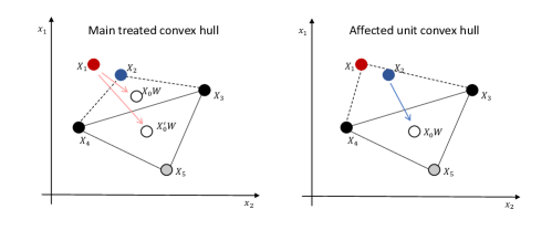
In Figures 3 and 4, we graphically represent possible scenarios from the point of view of unit 1 (“main treated” unit) on the left side and unit 2 (“potentially affected” unit) on the right side. Without loss of generality, we assume to observe only two predictors ( and ) for each unit. , i.e., the red point, is the vector that includes the pre-intervention predictors of the “main treated” and , i.e., the blue point, is the vector that includes the pre-intervention predictors of the only affected unit. All other points represent the vectors of pre-intervention predictors of each “pure control” unit. When marked in black, they contribute to the synthetic control, whereas when marked in grey they do not contribute.
Figure 3 shows the scenario in which both the “main treated” and the “potentially affected” units lie inside the convex hull of the “pure control” units. In this case, one can reproduce only using “pure control” units. However, a closer look at the right side of Panel 3a reveals that including the “potentially affected” unit to reproduce the characteristics of the “main treated” unit allows the exclusion of the farthest “pure control” unit (unit 3), restricting the donor pool, and potentially reducing interpolation bias (see Abadie 2021). The same goes for the “potentially affected” unit: including the “main treated” in the donor pool allows the exclusion of unit 4, which lies farther away from unit 2.
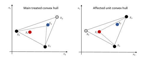
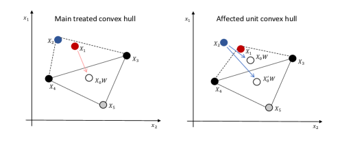
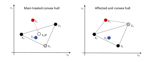
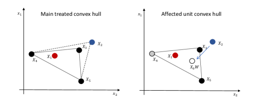
Figure 4 presents some scenarios in which only one unit between the “main treated” and the “potentially affected” unit lies inside the convex hull of the other and the “pure control” units. The left side of Panel 4a shows the case in which the “main treated” unit lies outside but close to the convex hull. Regardless of whether we exclude or include the “potentially affected” unit, we can only approximate . However, excluding unit 2 would lead to a bigger discrepancy between , therefore it is better to include it in the donor pool. On the right side of Panel 4a, we notice that the “potentially affected” unit lies outside the convex hull unless we include the “main treated” in its donor pool. Panel 4b shows a symmetric situation to that in Panel 4a. The left side of Panel 4c shows a scenario in which the “main treated” lies outside the convex hull and including unit 2 improves the approximation. The right side of Panel 4c shows a scenario in which unit 2 is always in the convex hull and including unit 1 the convex hull becomes bigger but it allows to improve approximation because unit 3 can be excluded. Panel 4d describes a scenario in which using iSCM clearly makes things worse. We suggest using iSCM when the “potentially affected” units receive substantial weight. It is less likely in this scenario.