Online Tree Reconstruction and Forest Inventory
on a Mobile Robotic System

Abstract

Terrestrial laser scanning (TLS) is the standard technique used to create accurate point clouds for digital forest inventories. However, the measurement process is demanding, requiring up to two days per hectare for data collection, significant data storage, as well as resource-heavy post-processing of 3D data. In this work, we present a real-time mapping and analysis system that enables online generation of forest inventories using mobile laser scanners that can be mounted e.g. on mobile robots. Given incrementally created and locally accurate submaps—data payloads—our approach extracts tree candidates using a custom, Voronoi-inspired clustering algorithm. Tree candidates are reconstructed using an adapted Hough algorithm, which enables robust modeling of the tree stem. Further, we explicitly incorporate the incremental nature of the data collection by consistently updating the database using a pose graph LiDAR SLAM system. This enables us to refine our estimates of the tree traits if an area is revisited later during a mission. We demonstrate competitive accuracy to TLS or manual measurements using laser scanners that we mounted on backpacks or mobile robots operating in conifer, broad-leaf and mixed forests. Our results achieve RMSE of $1.93\text{\,}\mathrm{cm}\text{/}$, a bias of $0.65\text{\,}\mathrm{cm}\text{/}$ and a standard deviation of $1.81\text{\,}\mathrm{cm}\text{/}$ (averaged across these sequences)—with no post-processing required after the mission is complete.

I Introduction

In traditional clear-cut forestry, plots of several hectares are felled at once when deemed ready for harvesting or thinning [18]. Modern forestry methods aim to minimize the impact on the forest ecosystem by carefully selecting which trees to cut—usually those fully grown or inhibiting the growth of other trees—which is called continous coverage forestry [17]. To support this approach and to assess its impact on the ecosystem requires the systematic data collection of tree locations and relevant tree traits, forest inventories, which enable the construction of high-fidelity digital twins of the forest, known as marteloscopes. For producing these marteloscopes, foresters and ecologists traditionally measure the tree traits manually, which is time-consuming and limits the set of tree traits that can be measured.

In order to address these challenges, methods based on terrestrial laser scanning (TLS) enabled a systematic and accurate acquisition of forestry data. However, they need periodic repositioning of the laser device through the forest, which increases data acquisition time and requires resource-heavy post-processing to determine the forest traits. In addition, vast amounts of raw data are generated, which reach up to $20\text{\,}\mathrm{GB}\text{/}\mathrm{ha}$. Alternatively, mobile laser scanners (MLS) have a much lower acquisition time as the sensor continuously moves, e.g. on a mobile robot. MLS methods, however, incur a compromise in sensor accuracy—a TLS sensor achieves millimeter measurement accuracy while MLS scanners are in the centimeter range. As a result, MLS mapping systems suffer from drift in pose estimation.

To address the issues of file size and post-processing time, we propose to amortize the post-processing time by performing the reconstruction online, during data acquisition. This way, we give immediate feedback on the scanning quality and coverage, and produces a marteloscope immediately after the session ends. In our initial approach, Proudman et al. [22] attempted to achieve this by detecting trees at the sensor rate of the LiDAR and then fusing and correcting the estimates upon loop closure. This required several simplifications in the tree detection and modeling to cope with the sensor frequency, consequently producing inferior reconstructions. This—in combination with the sparsity of single scans—did not allow for faithful estimation of tree parameters.

In this work, we address these limitations and introduce a real-time system to create online forest marteloscopes on mobile robotic platforms. We use a combination of a pose graph SLAM system and a custom Tree Manager module to segment trees, associate measurements over time, and maintain global consistency. Once there are enough measurements available for a tree, it is reconstructed employing a Hough-inspired filtering procedure and a model-averaging reconstruction algorithm. Although running with limited compute resources, our pipeline produces faithful estimates of important tree traits faster than point clouds are acquired. Thus, our approach can be considered the first algorithm that enables real-time forest inventory with reconstructions available as soon as the measurement session has ended.

In summary, we present four contributions in our work: Our approach is able to (i) extract relevant tree traits online with accuracy competitive to state-of-the-art post-processing approaches, (ii) produce a globally consistent tree map of the forest which is built incrementally and updated in real-time, (iii) robustly detect and fit stacks of oblique cone frustums in the presence of heavy noise, which has been tested on datasets of different tree compositions, (iv) run on a mobile system - either a quadruped robot or a human-carried backpack. We have extensively tested our approach using forest data from the UK, Switzerland, and Finland.

II Related Work

II-1 Terrestrial Laser Scanning

The ecology and forestry community has developed a mature body of literature describing tools for building forest inventories using TLS [13, 12]. Methods building high-fidelity models usually employ highly engineered pipelines based on cover sets, clustering, sorting, and cylinder fitting algorithms to reconstruct the tree components [24, 11]. While these methods aim to extract maximum information from point clouds, they often incur substantial computational costs, with processing times up to half an hour per tree [24].

Other methods focus on building a lower fidelity model of the tree that only considers the stem. These approaches typically begin with Voronoi clustering of the trees [20], followed by individual stem reconstruction [3, 20]. Methods employing clustering of cover sets can reconstruct multiple trees from the point cloud directly [19].

Stem models usually consist of stacked oblique cone frustums [3, 20, 14] or a cubic spline [19] that interpolates the diameters, enabling the tree diameter to be interpolated and extrapolated along its height. These methods involve a reconstruction of a stack of circles. An effective approach has been to filter outliers that are not in keeping with three lower circles [14, 19]. When coupled with terrain detection, these methods offer an automated procedure to estimate the diameter at breast height (DBH) and other tree traits, such as the total merchantable volume [19, 20] and stem curvature [21]. They achieve a Root Mean Square Error (RMSE) for the DBH estimate as low as $7.3\text{\,}\mathrm{mm}\text{/}$ [19].

While these approaches offer high-fidelity representations and accurate reconstructions, their computational cost makes them unsuitable for online processing. So instead, in this paper, our emphasis lies on Mobile Laser Scanning, enabling convenient data generation and evaluation by moving the sensor through the plot—in a fraction of the time.

II-2 Mobile Laser Scanning

Other researchers also focus on improving MLS systems, deploying them on backpacks [22, 10] or drones [9]. A notable advantage of MLS systems is that they achieve better coverage of the trees by continuously scanning from multiple perspectives [1]. The primary challenge facing MLS pipelines, however, is the complex alignment procedure of point clouds. While short-term missions may suffice with simple integration of odometry for alignment [23], longer missions need a SLAM system to correct sensor drift in the odometry [10, 9, 1]. As we design our pipeline to work with long-duration scans, we also employ a SLAM system to ensure global consistency. Once a globally consistent map is obtained, MLS pipelines employ various methods to generate a digital terrain model (DTM) to standardize the clouds by height. This is followed by clustering using learned approaches [23], the Watershed Algorithm [9], the QuickShift++ Algorithm [16], or euclidean clustering [22].

For modeling a tree, MLS methods usually represent the stem as a single cylinder [22], a stack of oblique cone frustums [1, 15, 9], or polynomial curves [10, 9] fitted to a stack of circles. The most promising results are achieved by curve models with RMSE for the DBH of $0.6\text{\,}\mathrm{cm}\text{/}$. Non-curve-based methods achieve an RMSE for the DBH as low as $1.14\text{\,}\mathrm{cm}\text{/}$ [20]. All these methods process point clouds in post-processing after acquiring all data and leaving the forest. To support foresters in gathering high-quality data and reduce reconstruction time, our focus is on an online approach that provides a real-time visualization as the map and reconstructions are being generated.

III Method

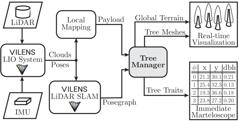
Figure 1: Overview of our proposed online tree reconstruction pipeline. The central Tree Manager is fed with payload clouds from the local mapping module as well as the pose graph from the LiDAR SLAM system. It generates a real-time visualization and constructs a marteloscope.

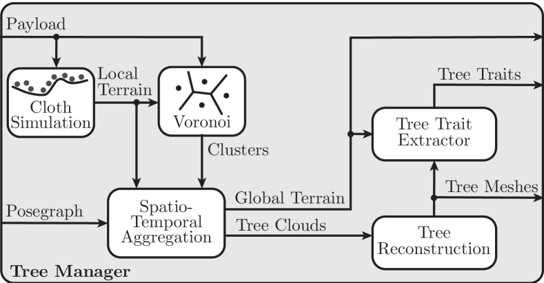
Figure 2: Overview of the Tree Manager module. Terrain models are produced by a cloth simulation filter (CSF) and clusters arecomputed by a Voronoi-inspired algorithm. We aggregate them over time in a globally consistent manner using the SLAM pose graph. After reconstruction of the trees, we can extract important tree traits.

The pipeline we propose, as shown in (Fig. 2), builds on top of our pose graph SLAM system, which is fed by a LiDAR inertial odometry (LIO) module [26]. The local mapping module integrates point clouds to local submaps—data payloads—to increase density. A constant stream of payloads is the input to our Tree Manager (Fig. 2). The Tree Manager builds a Local Terrain Model and segments the trees. It uses the SLAM pose graph to aggregate measurements for tree instances in a spatio-temporal manner. With enough data, the tree is reconstructed and tree traits are extracted. The result of the pipeline is an online visualization of the map and a marteloscope immediately after data acquisition.

In our work, we use two coordinate frames: The map frame $\mathtt{M}$ for final reconstruction and the moving sensor frame $\mathtt{S}^{t}$ at timestamp $t$, for representing raw measurements.

III-A Local Mapping

Using the poses provided by the odometry and by integrating loop closures, VILENS builds a globally consistent and time-varying pose graph. This graph comprises stamped transformations ${}^{\mathtt{M}}\mathbf{T}_{\mathtt{S}^{t}}$ from sensor frame to map frame.

The LIO system outputs a point cloud at a rate of 10 Hz. Although the density of an individual scan is sufficient for odometry, it is not dense enough for faithful tree reconstruction. This is why we integrate individual measurements along a trajectory of $20\text{\,}\mathrm{m}\text{/}$ using the poses provided by the LIO, which we call a payload (abbreviated pl). We represent the payload in $\mathtt{S}^{t}$ with $t$ referring to the center timestamp of the $20\text{\,}\mathrm{m}\text{/}$ long trajectory. Using $t$ as a unique identifier, the payload cloud is attached to the SLAM pose graph. To reduce computational load, we first downsample the cloud using a voxel filter with a resolution of $1\text{\,}\mathrm{cm}\text{/}$. Secondly, we remove points further away than $r_{\text{pl}}=20\,\textup{m}$ as they are noisier than short-range points. After reducing the point count, we call the stamped payload cloud ${}^{\mathtt{S}^{t}}\mathcal{P}_{\text{pl}}$.

III-B Terrain Model based on Cloth Simulation Filtering

For modeling sloping forest terrain, we generate a local DTM ${}^{\mathtt{S}^{t}}\mathcal{M}_{\textup{DTM}}^{\text{local}}$ for ${}^{\mathtt{S}^{t}}\mathcal{P}_{\text{pl}}$ using the cloth simulation filter proposed by Zhang et al. [27]. We associate it with the SLAM pose graph so that we can combine the set of ${}^{\mathtt{S}^{t}}\mathcal{M}_{\textup{DTM}}^{\text{local}}$ into a global DTM ${}^{\mathtt{M}}\mathcal{M}_{\textup{DTM}}^{\text{global}}$ to extract tree traits (Sec. III-D).

III-C Voronoi-Inspired Tree Segmentation

To cluster the trees, we propose an adaptation to the algorithm introduced by Cabo et al. [3], where the authors clustered TLS point clouds. Cabo et al. normalized the floor height of the point cloud and cropped it between heights where they expected no foliage. After clustering the cropped sections, they fit tree axes to the clusters using principal component analysis, and ultimately assigned points to tree instances by distance to the closest tree axis following the Voronoi paradigm.

We extend their approach by introducing non-maximum suppression (NMS), where we fit tree axes to three cropped sections—instead of one—and choose the best fit using a fitness function. After normalizing the floor height of ${}^{\mathtt{S}^{t}}\mathcal{P}_{\text{pl}}$ using ${}^{\mathtt{S}^{t}}\mathcal{M}_{\textup{DTM}}^{\text{local}}$, we align the cloud with gravity by transforming it into the map frame $\mathtt{M}$. Now, we crop the cloud at three height intervals and cluster the crops using Density-Based Spatial Clustering of Applications with Noise (DBSCAN) [6] resulting in cluster point clouds $\{\mathcal{P}_{\text{cluster}}^{k^{t}}\}_{k^{t}}$. We fit a cylinder to each cluster using two Hough-RANSAC circles (Sec. III-E) fitted to slices on the top and bottom of the cluster. After this, we use the fitness function $\phi_{k^{t}}$ described in Eq. (1), employing the distance $d(p_{i},a_{k^{t}})$ from point $p_{i}\in\mathcal{P}_{\text{cluster}}^{k^{t}}$ to axis $a_{k^{t}}$, the cylinder’s radius $r_{k^{t}}$, and the Heaviside function $H(x)$. This function penalizes points inside the cylinder and prefers points close to its surface.

Using $\phi_{k^{t}}$, we apply NMS to select the best cylinders, whose main axes build the final set of axes $\{a_{\text{NMS}}^{l}\}_{l}$.

$$\phi_{k^{t}}=\frac{N_{1.2*r_{k^{t}}}}{{N_{0.5*r_{k^{t}}}}}\;\;\;\;N_{\theta}=\sum_{i}H(d(p_{i},a_{k^{t}})-\theta)$$ (1)

Finally, we compute distances from every point in the height-normalized point cloud to all $a_{\text{NMS}}^{l}$. After undoing the height-normalization and transforming the point clouds back into $\mathtt{S}^{t}$, we arrive at cluster point clouds ${}^{\mathtt{S}^{t}}\mathcal{P}_{\text{cluster},l}$.

III-D Spatio-Temporal Aggregation

In order to keep the map globally consistent over time, the tree manager uses ${}^{\mathtt{M}}\mathbf{T}_{\mathtt{S}^{t}}$ from the SLAM pose graph to transform raw measurements, which are stored in the sensor frame $\mathtt{S}^{t}$, into map frame $\mathtt{M}$. Whenever loop closures occur, the SLAM system updates ${}^{\mathtt{M}}\mathbf{T}_{\mathtt{S}^{t}}$, which keeps the pose graph and thereby our reconstructions globally consistent.

To build ${}^{\mathtt{M}}\mathcal{M}_{\textup{DTM}}^{\text{global}}$, which is used to locate the measurement height for the DBH, all local DTMs are converted into map frame $\mathtt{M}$. For smooth blending of the local models, we generate weights for every vertex of the DTMs using the function described in Eq. (2). It enables a C0-continuous transition between local DTMs using their width $w_{\textup{DTM}}$ and length $l_{\textup{DTM}}$ as well as the sensor position $\bm{x}_{\text{sensor}}$. Using rays sampled on a regular grid and an efficient ray-to-mesh intersection algorithm by Wald et al. [25], we build ${}^{\mathtt{M}}\mathcal{M}_{\textup{DTM}}^{\text{global}}$ by computing the weighted average of the local DTM heights for every ray.

$$w(\bm{x})=1-\frac{||\bm{x}-\bm{x}_{\text{sensor}}||_{2}}{\min(l_{\text{DTM}},w_{\text{DTM}})/2}$$ (2)

In addition to ${}^{\mathtt{M}}\mathcal{M}_{\textup{DTM}}^{\text{global}}$, the Tree Manager also maintains a database of tree instances. Whenever a clustering result becomes available, every cluster ${}^{\mathtt{S}^{t}}\mathcal{P}_{\text{cluster},l}$ is compared to the current database of trees. ${}^{\mathtt{S}^{t}}\mathcal{P}_{\text{cluster},l}$ is either added to an existing tree instance if it is close, or a new instance is created. Using the timestamps of the clusters for association, the Tree Manager regularly realigns all clusters in all trees using the most recent ${}^{\mathtt{M}}\mathbf{T}_{\mathtt{S}^{t}}$ from the SLAM pose graph.

To make the best use of the available compute resources, we require certain coverage conditions on every tree before it is reconstructed. The first condition is a maximum distance of the sensor from the tree of at least $d^{\text{reco}}_{\text{min}}$, which ensures that the LiDAR with its limited field of view has scanned points sufficiently high up the tree. The second condition is the coverage angle $\alpha^{\text{reco}}_{\text{min}}$ making sure that there are sufficient measurements from around the tree. In our experiments values of $d^{\text{reco}}_{\text{min}}=10m$ and $\alpha^{\text{reco}}_{\text{min}}=\pi$ gave reasonable results.

III-E Tree Reconstruction and Tree Trait Extraction

For clustering and reconstruction tasks, we need an efficient algorithm to fit circles to 2D slices of point clouds, even in the presence of outliers, such as leaves or branches. As proposed by de Conto et al. [4], an effective algorithm for this is the Hough Transform [8] applied to circles [5]. This method detects circular shapes in a bitmap of edges by using circles of variable centers and radii to vote within a discretized Hough space. For circles, the Hough space is three-dimensional with two coordinates for the circle center and one for the radius. To apply the classical approach to Hough fitting in the point cloud setting, one has to rasterize the points by aggregating them into a bitmap. Although this algorithm is generally considered robust for fitting circles, its performance was poor in the presence of MLS noise.

To tackle this, we propose an adaptation to the Hough algorithm by considering a continuous Hough space and combining that with the idea of RANdom SAmple Consensus (RANSAC) [7], which we call Hough-RANSAC.

By translating the classical Hough algorithm to a grid of infinitesimal resolution, we obtain a three-dimensional continuous Hough space $(x,y,r)^{T}\in\mathbb{H}=\mathbb{R}^{2}\times\mathbb{R}_{+}$ where we can natively represent a 2D point cloud as an input for the Hough algorithm. The casting of votes happens by constructing a cone for every point $\bm{p}^{j}$ whose main axis is aligned with the radius axis of the Hough space. The x- and y- coordinates of $\bm{p}^{j}$ match the center of the cone in the Hough space (Fig. 4). The slope of the cone is equal to $1$.

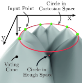
Figure 3: Every point in the slice casts votes in the Hough space along a cone. Wherever there is a high density of cone intersections, there is a good candidate fit for a circle.

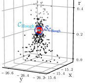
Figure 4: Point cloud $\mathcal{P}_{\text{Hough}}$ of intersections of cone triplets. At a point $\mathcal{C}_{\text{Hough}}$ with the sphere $\mathcal{S}_{\mathcal{C}_{\text{Hough}}}$ around it containing many intersections (marked in red), a good circle fit can be found.

After constructing a voting cone for every input point, the optimal circle fit $\mathcal{C}_{\text{Hough}}$ is determined as a point in continuous Hough space $\mathbb{H}$. This is achieved by locating a point in $\mathbb{H}$ where, within a sphere $\mathcal{S}_{\mathcal{C}_{\text{Hough}}}$ of fixed radius around $\mathcal{C}_{\text{Hough}}$, the most voting cones intersect, i.e. the most votes are cast. The radius of this sphere can be tuned to balance robustness against computational cost. As there is no explicit solution for $\mathcal{C}_{\text{Hough}}$, instead of intersecting cones with the sphere, we first intersect the cones with each other. With the main axes of all cylinders aligned, the point cloud $\mathcal{P}_{\text{Hough}}$ of all intersection points of cones can be found by finding the intersecting points of all possible triplets of voting cones. It can be shown that this intersection point corresponds to the Hough representation of the circle fitted through a triplet of points, which can be explicitly and efficiently calculated. Now, $\mathcal{C}_{\text{Hough}}$ can be found as the point where $\mathcal{S}_{\mathcal{C}_{\text{Hough}}}$ contains the most points in $\mathcal{P}_{\text{Hough}}$ (Fig. 4). As it is infeasible to compute all intersections, which scale with $\mathcal{O}(N^{3})$ with $N$ being the number of input points, we randomly sample triplets of points to approximate $\mathcal{P}_{\text{Hough}}$. This follows the paradigm established by the RANSAC algorithm.

This algorithm has the advantage of a continuous Hough space, but it comes at the cost of its runtime scaling proportionally to the number of sampled triplets. We tackle this problem by weighting the sampling of triplets by the inverse distance of a point to its nearest neighbor. Thereby we could reduce the number of samples while still maintaining faithful circle fits. For ablation studies, please refer to Sec. IV-C1.

Once the reconstruction criteria of the Tree Manager are fulfilled, we reconstruct the tree as a stack of oblique cone frustums between circles reconstructed at regular heights (Fig. 6). For each slice and cluster, we fit a Hough-RANSAC circle to filter out the outliers by distance. To optimize computational efficiency, we constrain the Hough space to consider only circles close to the previous circle in the x-y plane of $\mathtt{M}$. For this to work reliably, we need a robust initialization, which we achieve by using a non-maximum suppression (NMS) on the first three reconstructions.

In order to fit a circle to filtered slices, we follow the approach of Hyyppä et al. [10] who use intermediate circle fit to align the clusters. We employ the explicit least-squares circle fitting algorithm proposed by Bullock et al. [2] to fit the final circle to the point cloud of aligned clusters.

For visualization purposes, we also generate canopy meshes. These can be efficiently computed by fitting a convex hull to all canopy points. We treat points more than $2\text{\,}\mathrm{m}\text{/}$ away from ${}^{\mathtt{M}}\mathcal{M}_{\textup{DTM}}^{\text{global}}$ and greater than twice the diameter away from the stem axis as canopy points.

Once reconstructions of terrain and trees are available, we visualize them in real-time, which enables assessment of the scanning quality and the coverage of the plot. Immediately after the mapping session ends, we export the results into an industry-standard representation for a marteloscope.

IV Experimental Evaluation

The focus of this work is the implementation of a real-time pipeline that reconstructs individual trees and extracts their tree traits. We present our experiments to show the capabilities of our method and to support our key claims, which are: (i) The extraction of relevant tree traits with accuracy competitive to state-of-the-art approaches, (ii) the generation of a globally consistent map of the forest, (iii) the robust fitting of oblique cone frustums to the trees in the presence of heavy sensor noise (iv) the ability to run on a mobile system.

	Plot	Conifer	Mixed	Deciduous	All
Detection Precision		98.3%	97.4%	98.6%	98.1%
DBH	RMSE [cm]	1.18	2.22	2.38	1.93
	Bias [cm]	0.02	0.34	2.05	0.65
	Std [cm]	1.17	2.18	1.04	1.81
RMSE Stem	Diameter [cm]	2.91	3.14	3.12	3.02
	Center [cm]	5.78	9.56	14.88	8.05
Mean Height	Ours [m]	8.36	6.30	3.30	6.12
	TLS [m]	17.16	15.22	5.94	10.22

TABLE I: Evaluation of our pipeline on three different plots. We report the RMSE of DBH estimates (relative to manual measurements) and the RMSE of the stem diameter and curvature measured along the entire stem (relative to a TLS based model). Additionally, we measured the mean height of the reconstructed stems and the detection precision of the clustering algorithm.

IV-A Tree Trait Estimation Accuracy

The first experiment evaluates the quality of our reconstructions and demonstrates that we can estimate tree traits with accuracy competitive with the state of the art. We considered three plots located in a forest in Stein am Rhein, Switzerland consisting of coniferous (58 trees), broad-leaf (163 trees) and a mixture of the two (70 trees). We expect conifer trees with large diameters and a sparse under-canopy to be easier to reconstruct than broad-leaf trees with more vegetation close to the ground as well as a complex branching structure.

The campaign was executed in March 2023 which involved MLS scanning with our Mobile Mapping System and manual measurements of the DBH by a team of professional foresters. We use these manual measurements as a ground truth to compare our DBH estimates to. We also want to assess the location of the stem’s center as well as the diameter of the tree trunk along the entire height, which we call stem curve. For this assessment, we need more descriptive measurements, which we obtain by building tree models from TLS scans with a resolution of $1\text{\,}\mathrm{cm}\text{/}$. For this experiment, we evaluated our system by simulating online data acquisition and tree reconstruction after data acquisition has ended.

IV-A1 Detection Precision

We started by evaluating our clustering algorithm to determine if we were able to detect all the trees present using the MLS data. As reported in Tab. I, our method was able to detect 98.08 % of all trees.

IV-A2 DBH Estimation

Next, we assessed the accuracy of our DBH estimates. For ground truth, we used the manual reference measurements of the tree diameters conducted by the foresters at a height of $1.3\text{\,}\mathrm{m}\text{/}$ above the ground, which we associated with the MLS scans using an AprilTag-based matching system. We report the results in Tab. I and visualize the results in Fig. 6. As expected, Tab. I shows that estimates for conifer trees are the most accurate with an RMSE of $1.18\text{\,}\mathrm{cm}\text{/}$, while the broad-leaf trees are the most challenging with an RMSE of $2.38\text{\,}\mathrm{cm}\text{/}$. The mixed plot is in between with an RMSE of $2.22\text{\,}\mathrm{cm}\text{/}$.

IV-A3 Stem Curve Estimation

Additionally, we evaluated the accuracy of our estimates of the entire stem curve by comparing our circle centers and diameters along the stem to tree models based on the TLS measurements. To build these models, we sliced the TLS tree clouds at regular intervals, annotated stem points and fitted circles to them in the least-squares sense. In Tab. I, we report an RMSE of diameter estimates along the stem of $3.02\text{\,}\mathrm{cm}\text{/}$ and an RMSE of the stem curvature of $8.05\text{\,}\mathrm{cm}\text{/}$—averaged over all plots.

IV-A4 Tree Height

Finally, we compared the heights of the reconstructed stems. For the TLS measurements, the stem cross-section could no longer be reliably estimated above heights of $10.22\text{\,}\mathrm{m}\text{/}$, our reconstructions could only estimate up to an average height of $6.12\text{\,}\mathrm{m}\text{/}$ (Tab. I). We attribute this to the sensor configuration, which has a limited field of view and thus cannot measure high up the tree.

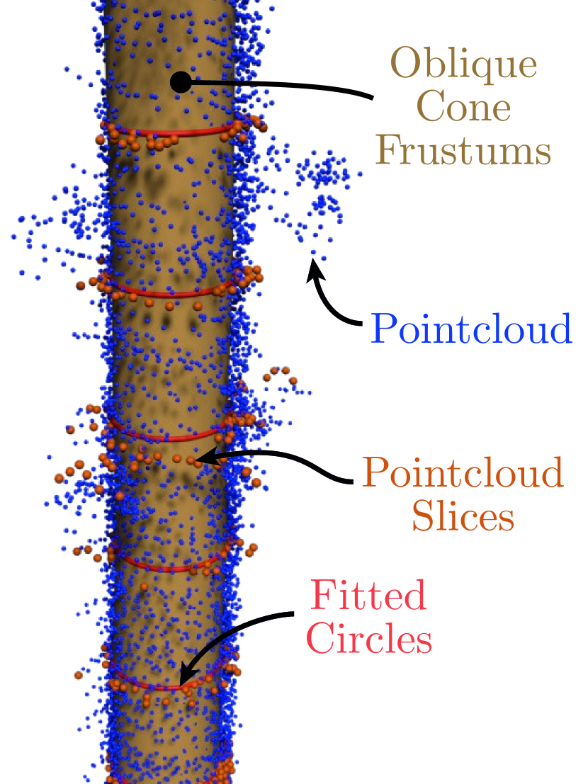
Figure 5: Stem reconstruction as a stack of oblique cone frustums.

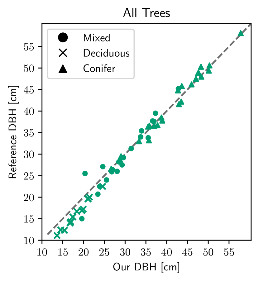
Figure 6: Scatter plots of the DBH estimates of our reconstructions against reference measurements.

IV-B Global Consistency

We designed the second experiment to demonstrate the importance of having a SLAM system ensuring globally consistent maps. For that, we let the pipeline run on the conifer plot again, but this time we disabled the trajectory updates in the Tree Manager. We did not disable the loop closures for the SLAM system, as drift accumulated over the entire trajectory would have made tree associations impossible. This implies that this experiment only considers the effect of the odometry drift in between loop closures.

Visually, the misalignment of the point clouds is shown in Fig. 8, but because of the realignment procedure described in Sec. III-E, our pipeline could still reconstruct stems.

A second effect is the failure of our pipeline to reliably merge tree clusters into a single tree instance (Fig. 8). This is due to the odometry drift being larger than our distance threshold for merging.

Ultimately, disabling loop closures in the tree manager should cause a reduction in the quality of the stem curve, which becomes apparent in Tab. II. We report a significant decrease of the RMSE in fitting the stem curve, which is to be expected if the point clouds are severely misaligned.

Figure 7: Incorrect tree association prior to a loop closure. Unique trees are represented as two different instances (different hues).

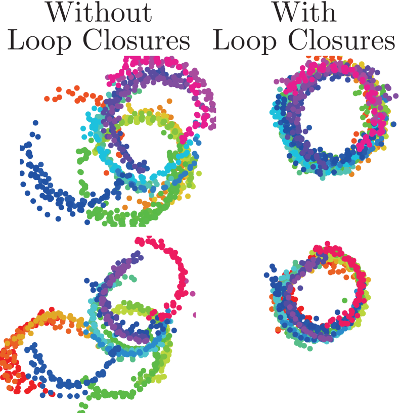
Figure 8: Misaligned cluster point clouds due to odometry drift. Loop closure corrections are able to realign them.

RMSE [cm]	DBH	Stem Curve	Stem Diameter
w/o loop closures	5.85	35.61	3.76
w/ loop closures	1.18	4.65	2.82

TABLE II: Comparison of running the pipeline with or without loop closures. Evaluated is the RMSE in the fitting of DBH, stem curve and stem diameter. All results are averaged over three runs.

IV-C Ablations

We designed a third set of experiments to demonstrate the benefit of other central components of our pipeline and their impact on reconstruction quality.

IV-C1 Hough-RANSAC

To demonstrate the value of the Hough-RANSAC algorithm, we compared it with the classical Hough algorithm, regular RANSAC fitting, and RANSAC*, where we applied the density-weighted subsampling procedure as described in Sec. III-E. For RANSAC and Hough-RANSAC we used 500 algorithm iterations.

In Tab. III, we report the RMSE of the DBH estimates for all ablations averaged over three runs on all three datasets. Hough-RANSAC outperforms the alternatives in terms of RMSE. Regarding timing, the classical Hough algorithm is faster, which we attribute to a less expensive mechanism for vote aggregation in the Hough space.

In Fig. 9, we present a qualitative analysis to give an intuition for why regular RANSAC and the Hough algorithm are inferior. Firstly, the Hough algorithm tends to overestimate the diameter of a cluster. Secondly, regular RANSAC struggles in the presence of branches or other sources of noise. We attribute both of these phenomena to the low sampling density of our point clouds, which increases the relative impact of noise. This biases the inlier counting mechanism of Hough and RANSAC towards larger circles. Meanwhile, Hough-RANSAC with a more robust mechanism for inlier detection, does not suffer from this bias.

Algorithm	RMSE [cm]				Time [ms]
	Conifer	Deciduous	Mixed	All
Hough	8.43	12.45	5.22	7.68	115
RANSAC	5.81	3.48	2.69	4.27	247
RANSAC*	2.78	3.88	2.67	3.26	275
Hough-RANSAC	1.18	2.38	2.22	1.93	191

TABLE III: Ablation study for different variants of robust circle fitting. We report the RMSE of the DBH estimates for the different versions averaged over three runs across all three of our datasets. We also report the timing of the algorithms.

Hough

RANSAC

Hough-RANSAC

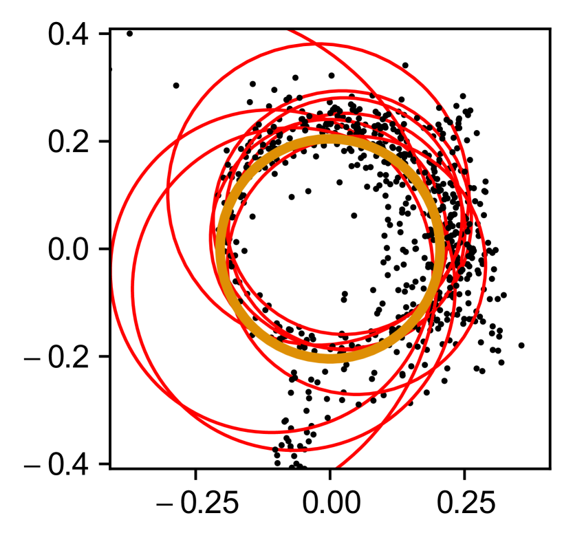
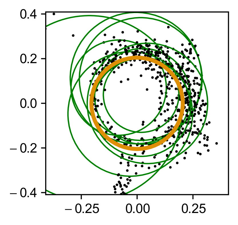
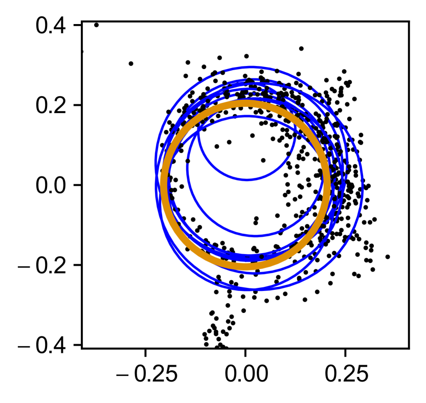
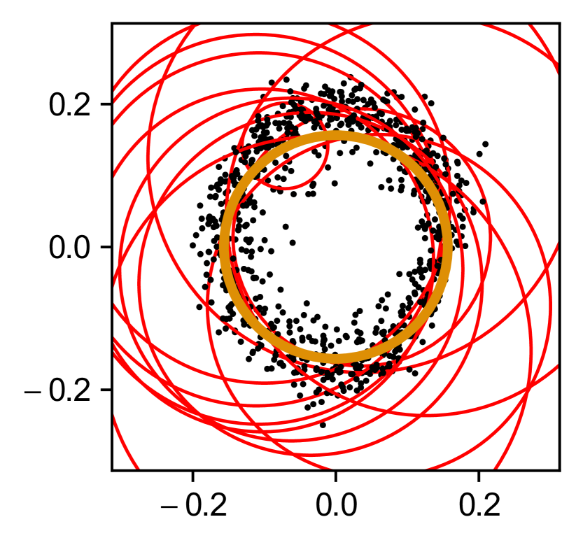
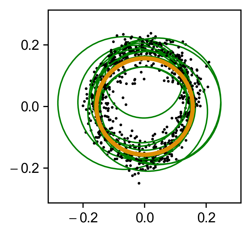
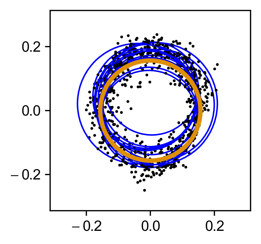
Figure 9: Examples of circle estimates on two point clouds with noise. The Ransac and Hough circle fit overestimates the diameter. Hough-RANSAC is able to fit the circle more accurately. The TLS circle fit is shown in orange. Note that the black points represent points from different clusters as in Fig. 8

.

IV-C2 Coverage Angle

This experiment was conducted to support our assumption that larger coverage angles, i.e. the range of directions the tree is scanned from, are beneficial for reconstruction quality. We reconstructed every tree of the three plots several times, each time removing clusters and noting the reduced coverage angle. We grouped results in buckets of $20^{\circ}$ increments and for each bucket computed the RMSE of diameter estimates along the stem curve with respect to the TLS dataset. We note a clear trend where increasing the coverage angle decreases the error of the estimate (Fig. 10).

This suggests that moving the sensor through the plot and measuring the trees from different angles is beneficial for accurate stem reconstruction.

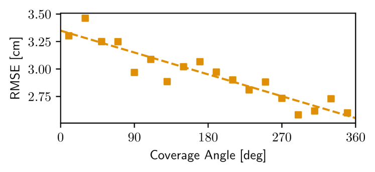
Figure 10: Accuracy of the DBH estimates as a function of coverage angle. As more of the tree is observed the DBH RMSE decreases.

IV-D Performance

This experiment explores the computation time of the real-time pipeline. We evaluated the runtime on a Simply NUC Topaz 3 featuring a Core i7-1165G7 with 4 cores, a base frequency of 2.8 GHz, and $32\text{\,}\mathrm{GB}\text{/}$ of RAM. Payload clouds are accumulated over $20\text{\,}\mathrm{m}\text{/}$, which on average took $19.8\text{\,}\mathrm{s}\text{/}$.

Fig. 12 presents the average runtime of the components of our pipeline for our different datasets. With an overall mean runtime of $9.69\text{\,}\mathrm{s}\text{/}$ and a standard deviation of $4.41\text{\,}\mathrm{s}\text{/}$, the algorithm is able to run approximately twice as fast as the capture frequency. Note that processing the deciduous plot consumes more time than the other two, which is due to the higher tree stem density. Across all datasets, the computationally most expensive component is the Tree Manager, which handles the reconstructions.

We also report system memory usage (Tab. IV) which, with an average of $5.69\text{\,}\mathrm{GB}\text{/}$, is well within the capabilities of our system. Perhaps the biggest advantage of our approach is in storage space. The average storage requirements of the final output data are in the range of $160\text{\,}\mathrm{MB}\text{/}$ for $0.7\text{\,}\mathrm{h}\mathrm{e}\mathrm{c}\mathrm{t}\mathrm{a}\mathrm{r}\mathrm{e}$ including the point clouds of every tree, and only $6\text{\,}\mathrm{MB}\text{/}$ when storing just the reconstruction results. This compares to $13.5\text{\,}\mathrm{GB}\text{/}$ for the raw data and hundreds of gigabytes for a traditional TLS system, which makes our system three orders of magnitude more efficient in terms of storage. This detail is critical as data acquisition is arduous and done in remote locations. Furthermore, compared to the intrinsic value of the raw measurements, the cost of storage is immense.

IV-E Real-time Demonstration on ANYmal Robot

In order to demonstrate this capability running live on a robot, we carried out a field trial in the Forest of Dean, UK. We used the ANYmal quadruped robot to autonomously carry the Mobile Mapping System through the forest with all reconstructions carried out in real-time and visualized online. This demonstration is presented in Fig. 11 and the supplementary video. (A complete description of the robot autonomy system is outside the scope of this paper.)

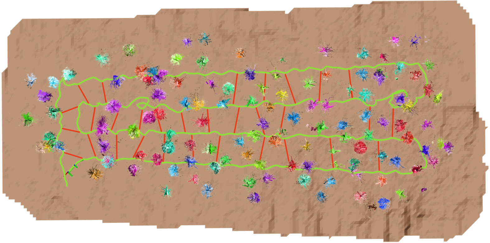
Figure 11: Fully autonomous mission through a plot of the Forest of Dean with the ANYmal quadruped autonomously navigating the forest following a lawnmower pattern. On board the Mobile Robot, our pipeline created an online forest inventory which was visualized for the operators in real-time. Note the pose graph (green) being corrected using loop closures (red).

		Conifer	Deciduous	Mixed
Memory		$5.18\text{\,}\mathrm{GB}\text{/}$	$6.75\text{\,}\mathrm{GB}\text{/}$	$5.15\text{\,}\mathrm{GB}\text{/}$
Storage	w/ clouds	$158.0\text{\,}\mathrm{MB}\text{/}$	$187.7\text{\,}\mathrm{MB}\text{/}$	$143.1\text{\,}\mathrm{MB}\text{/}$
	w/o clouds	$1.5\text{\,}\mathrm{MB}\text{/}$	$9.2\text{\,}\mathrm{MB}\text{/}$	$8.0\text{\,}\mathrm{MB}\text{/}$

TABLE IV: Memory (during runtime) and Storage requirements (afterwards) for final output data (with and without storing the point clouds for every tree).

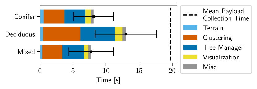
Figure 12: Runtime of individual components of our pipeline given by mean and standard deviation. With a time budget of $19.8\text{\,}\mathrm{s}\text{/}$ per payload, our approach runs almost twice as fast as required.

V Conclusion

In this paper, we presented a novel approach for real-time tree inventory and reconstruction in forest environments. Our method incrementally reconstructs hectare-sized forest plots by accumulating a local submap (a payload) and clustering and reconstructing tree instances within it. Payloads are incrementally merged and global consistency of the full map is maintained by leveraging a pose graph SLAM system.

Compared to other state-of-the-art methods that compute the result in post-processing, our approach produces a dataset of tree instances and tree traits (such as the DBH and stem curve) during data acquisition. Additionally, we can report the state of the reconstruction in real-time, helping the forester—or an autonomous robot—to adjust the mission to e.g. increase coverage for better reconstructions.

We evaluated our pipeline on three forest datasets with different compositions and showed that we can estimate tree traits with an accuracy competitive with the state of the art. Averaging across deciduous and conifer plantations, our method achieved an RMSE for DBH estimates of $1.93\text{\,}\mathrm{cm}\text{/}$.

Focusing on conifer plantations, our accuracy was measured as $1.18\text{\,}\mathrm{cm}\text{/}$ while a state-of-the-art method from Hyyppä et al. achieved an RMSE of $0.6\text{\,}\mathrm{cm}\text{/}$ [9]. We note that our approach required significantly less computation time as well as an order of magnitude cheaper hardware.

Using our three datasets we supported all claims made in this paper. The experiments suggest that online estimation of tree traits is feasible and can deliver faithful reconstructions of trees. For further development, our pipeline is a good starting point to use other sensor modalities to estimate more tree traits such as the tree species from RGB images.

Considering the light weight of the pipeline as well as the Mobile Mapping System itself, we believe that with improvements in remote sensing hardware, building online forest inventories can be a valuable tool to quickly generate accurate models of forests.

References

- [1] A. Bienert, L. Georgi, M. Kunz, H.G. Maas, and G. Von Oheimb. Comparison and combination of mobile and terrestrial laser scanning for natural forest inventories. Forests, 9(7), 2018.
- [2] R. Bullock. Least-squares circle fit. Developmental testbed center, 3, 2006.
- [3] C. Cabo, C. Ordóñez, C.A. López-Sánchez, and J. Armesto. Automatic dendrometry: Tree detection, tree height and diameter estimation using terrestrial laser scanning. International Journal of Applied Earth Observation and Geoinformation, 69:164–174, 2018.
- [4] T. de Conto, K. Olofsson, E.B. Görgens, L.C.E. Rodriguez, and G. Almeida. Performance of stem denoising and stem modelling algorithms on single tree point clouds from terrestrial laser scanning. Computers and Electronics in Agriculture, 143:165–176, 2017.
- [5] R.O. Duda and P.E. Hart. Use of the hough transformation to detect lines and curves in pictures. Communications of the ACM, 15(1):11–15, 1972.
- [6] M. Ester, H. Kriegel, J. Sander, and X.Xu. A density-based algorithm for discovering clusters in large spatial databases with noise. In Kdd, volume 96, pages 226–231, 1996.
- [7] M. Fischler and R. Bolles. Random Sample Consensus: A Paradigm for Model Fitting with Applications to Image Analysis and Automated Cartography. Commun. ACM, 24(6):381–395, 1981.
- [8] P.V. Hough. Method and means for recognizing complex patterns, December 18 1962. US Patent 3,069,654.
- [9] E. Hyyppä, J. Hyyppä, T. Hakala, A. Kukko, M.A. Wulder, J.C. White, J. Pyörälä, X. Yu, Y. Wang, J.P. Virtanen, O. Pohjavirta, X. Liang, M. Holopainen, and H. Kaartinen. Under-canopy uav laser scanning for accurate forest field measurements. ISPRS Journal of Photogrammetry and Remote Sensing (JPRS), 164:41–60, 2020.
- [10] E. Hyyppä, A. Kukko, R. Kaijaluoto, J.C. White, M.A. Wulder, J. Pyörälä, X. Liang, X. Yu, Y. Wang, H. Kaartinen, J.P. Virtanen, and J. Hyyppä. Accurate derivation of stem curve and volume using backpack mobile laser scanning. ISPRS Journal of Photogrammetry and Remote Sensing (JPRS), 161:246–262, 2020.
- [11] S. Krisanski, M.S. Taskhiri, S. Gonzalez Aracil, D. Herries, A. Muneri, M.B. Gurung, J. Montgomery, and P. Turner. Forest structural complexity tool—an open source, fully-automated tool for measuring forest point clouds. Remote Sensing, 13(22), 2021.
- [12] X. Liang, J. Hyyppä, H. Kaartinen, M. Lehtomäki, J. Pyörälä, N. Pfeifer, M. Holopainen, G. Brolly, P. Francesco, J. Hackenberg, H. Huang, H.W. Jo, M. Katoh, L. Liu, M. Mokrovs., J. Morel, K. Olofsson, J. Poveda-Lopez, J. Trochta, D. Wang, J. Wang, Z. Xi, B. Yang, G. Zheng, V. Kankare, V. Luoma, X. Yu, L. Chen, M. Vastaranta, N. Saarinen, and Y. Wang. International benchmarking of terrestrial laser scanning approaches for forest inventories. ISPRS Journal of Photogrammetry and Remote Sensing (JPRS), 2018.
- [13] X. Liang, V. Kankare, J. Hyyppä, Y. Wang, A. Kukko, H. Haggrén, X. Yu, H. Kaartinen, A. Jaakkola, F.Y. Guan, M. Holopainen, and M. Vastaranta. Terrestrial laser scanning in forest inventories. ISPRS Journal of Photogrammetry and Remote Sensing (JPRS), 115:63–77, 2016.
- [14] X. Liang, V. Kankare, X. Yu, J. Hyyppä, and M. Holopainen. Automated stem curve measurement using terrestrial laser scanning. IEEE Trans. on Geoscience and Remote Sensing, 52(3):1739–1748, 2014.
- [15] L. Liu, A. Zhang, S. Xiao, S. Hu, N. He, H. Pang, X. Zhang, and S. Yang. Single tree segmentation and diameter at breast height estimation with mobile lidar. IEEE Access, 9:24314–24325, 2021.
- [16] M. Malladi, T. Guadagnino, L. Lobefaro, M. Mattamala, H. Griess, J. Schweier, N. Chebrolu, M. Fallon, J. Behley, and C. Stachniss. Tree Instance Segmentation and Traits Estimation for Forestry Environments Exploiting LiDAR Data . In Proc. of the IEEE Intl. Conf. on Robotics & Automation (ICRA), 2024. Accepted.
- [17] B. Mason, G. Kerr, A. Pommerening, C. Edwards, S. Hale, D. Ireland, and R. Moore. Continuous cover forestry in british conifer forests. Forest Research Annual Report and Accounts, 2004:38–53, 2003.
- [18] J.D. Matthews. Silvicultural systems. Oxford University Press, 1991.
- [19] T.P. Pitkänen, P. Raumonen, and A. Kangas. Measuring stem diameters with tls in boreal forests by complementary fitting procedure. ISPRS Journal of Photogrammetry and Remote Sensing (JPRS), 147:294–306, 2019.
- [20] C. Prendes, C. Cabo, C. Ordóñez, J. Majada, and E. Canga. An algorithm for the automatic parametrization of wood volume equations from terrestrial laser scanning point clouds: application in pinus pinaster. GIScience & Remote Sensing, 58(7):1130–1150, 2021.
- [21] C. Prendes, E. Canga, C. Ordóñez, J. Majada, M. Acuna, and C. Cabo. Automatic assessment of individual stem shape parameters in forest stands from tls point clouds: Application in pinus pinaster. Forests, 2022.
- [22] A. Proudman, M. Ramezani, S.T. Digumarti, N. Chebrolu, and M. Fallon. Towards real-time forest inventory using handheld lidar. Robotics and Autonomous Systems, 157:104240, 2022.
- [23] X.L. Qiujie Li, Pengcheng Yuan and H. Zhou. Street tree segmentation from mobile laser scanning data. International Journal of Remote Sensing, 41(18):7145–7162, 2020.
- [24] P. Raumonen, M. Kaasalainen, M. Åkerblom, S. Kaasalainen, H. Kaartinen, M. Vastaranta, M. Holopainen, M. Disney, and P. Lewis. Fast automatic precision tree models from terrestrial laser scanner data. Remote Sensing, 5(2):491–520, 2013.
- [25] I. Wald, S. Woop, C. Benthin, G.S. Johnson, and M. Ernst. Embree: a kernel framework for efficient cpu ray tracing. ACM Transactions on Graphics, 33(4), jul 2014.
- [26] D. Wisth, M. Camurri, and M. Fallon. Robust legged robot state estimation using factor graph optimization. IEEE Robotics and Automation Letters, 4(4):4507–4514, 2019.
- [27] W. Zhang, J. Qi, P. Wan, H. Wang, D. Xie, X. Wang, and G. Yan. An easy-to-use airborne lidar data filtering method based on cloth simulation. Remote Sensing, 8(6), 2016.