Time-Optimal Flight with Safety Constraints and Data-driven Dynamics

Abstract

Time-optimal quadrotor flight is an extremely challenging problem due to the limited control authority encountered at the limit of handling. Model Predictive Contouring Control (MPCC) has emerged as a leading model-based approach for time optimization problems such as drone racing. However, the standard MPCC formulation used in quadrotor racing introduces the notion of the gates directly in the cost function, creating a multi-objective optimization that continuously trades off between maximizing progress and tracking the path accurately. This paper introduces three key components that enhance the MPCC approach for drone racing. First and foremost, we provide safety guarantees in the form of a constraint and terminal set. The safety set is designed as a spatial constraint which prevents gate collisions while allowing for time-optimization only in the cost function. Second, we augment the existing first principles dynamics with a residual term that captures complex aerodynamic effects and thrust forces learned directly from real world data. Third, we use Trust Region Bayesian Optimization (TuRBO), a state of the art global Bayesian Optimization algorithm, to tune the hyperparameters of the MPC controller given a sparse reward based on lap time minimization. The proposed approach achieves similar lap times to the best state-of-the-art RL and outperforms the best time-optimal controller while satisfying constraints. In both simulation and real-world, our approach consistently prevents gate crashes with 100% success rate, while pushing the quadrotor to its physical limit reaching speeds of more than 80km/h.

I Introduction

The last decade has seen a remarkable growth in the number of quadrotor applications. Many missions are time-critical, such as search and rescue, aerial delivery, flying cars, or space exploration [1, 2, 3]. Among them, drone racing has emerged as a testbed for research on time-optimal flight. Quadrotors are carefully engineered to push the limits of speed and agility, making drone racing an ideal benchmark for aerial performance and robustness at high speeds [4, 5].

State-of-the-art approaches to autonomous drone racing can be categorized into learning-based and optimization-based methods. Within learning-based methods, Reinforcement Learning (RL) has arisen as an attractive alternative to conventional planning and control algorithms, outperforming world-champion pilots [6, 7]. Unlike optimal control, RL uses data sampled through millions of trial-and-error interactions with the environment to optimize a controller. RL can manage sparse objectives and unstructured observation spaces, providing substantial flexibility and versatility in the controller design.

Figure 1: Long exposure picture of our quadrotor flying at more than 80km/h in a physical racing track. The safety set is shown in translucent white, expanding in gate-free regions and constricting at gate passages. The safety set is a crucial element of our approach, thanks to which we can consistently prevent gate collisions and achieve 100% success rate in real-world experiments, even when operating at the drone’s physical limits.

As shown in [7], RL can directly optimize a task-level objective, eliminating the need for explicit intermediate representations such as trajectories. Furthermore, RL can leverage domain randomization in simulation to cope with model uncertainty, allowing the discovery of more robust control responses. These advantages have facilitated numerous breakthroughs in pushing quadrotor systems to their operational limits through RL [7, 6]. However, despite the empirical success, RL controllers lack theoretical guarantees. Integrating safety considerations into machine learning frameworks, especially within RL, remains an area of ongoing research [8, 9]. The combination of optimization-based and learning-based architectures to enhance safety in RL is emerging as a prominent topic within the robotics community [10, 11, 12].

Conversely, optimization-based architectures have tackled the problem from a different perspective. In [13], the authors propose a method to find time-optimal trajectories through a predefined set of waypoints and show how they outperform expert drone-racing pilots. However, these trajectories take several hours to calculate, rendering them impractical for replanning in the face of model mismatch and unknown disturbances (e.g., drone model, gate positions, aerodynamic effects, wind gusts). Addressing this challenge necessitates an algorithm capable of generating time-optimal trajectories in real time. In [14, 15], a Model Predictive Contouring Control (MPCC) method is introduced to track non-feasible paths in a time-optimal fashion. By solving the complex time-allocation problem online at every time step, MPCC selects the optimal states and inputs that maximize the progress along the designated path. This approach yields a controller that shows great adaptation against model mismatch and unknown disturbances.

Several modifications to the MPCC cost function are necessary to adapt the MPCC formulation to the drone racing task. First, the notion of gates is introduced in the objective function by parameterizing the contour weight as a function of the progress. This comes with adding extra hyperparameters, which i) introduces a multi-objective cost function that forces a sub-optimal trade-off between performance and safety, ii) does not generalize to different gate configurations, and iii) requires complex tuning due to the increased number of parameters. Various strategies have been devised to address the tuning problem for contouring controllers. For instance, [16] employs a policy search technique to explore the high-level parameter space of the cost function. Similarly, [17] explores the parameter space using local Bayesian Optimization (BO). Although these methods have resulted in control capabilities surpassing those of human pilots, the approximations in the cost function are still exceedingly intricate, suggesting the possibility for more robust and scalable alternatives. Such alternatives would ideally achieve the desired outcomes by imposing constraints that consistently prevent gate collisions, avoiding the need to handcraft complex, high-parametric cost functions.

Previous works have aimed to tackle this issue by introducing a tunnel-shaped constraint set around the trajectory of the quadrotor [18, 19, 20]. In particular, [20] presents a tunnel-shaped constraint set by adapting the quadrotor’s dynamics into a local Frenet-Serret reference frame, which naturally gives rise to position constraints in the shape of a tunnel. The authors validate their approach in simulation and show that they can fly different tracks at high speeds within the confines of the tunnel.

Contributions

This paper introduces three key components that enhance the state-of-the-art MPCC formulation for drone racing. First, we provide safety guarantees in the form of a constraint and terminal set. The safety set is designed as a spatial constraint that prevents gate collisions in the form of a prismatic tunnel, similar to [20]. The terminal set consists of a periodic, feasible centerline. This combination provides guarantees of recursive feasibility and inherent robustness. Second, we augment the existing first principles dynamics with a residual term that captures complex aerodynamic effects and thrust forces learned directly from real-world data. Third, we use Trust-Region Bayesian Optimization (TuRBO), a state-of-the-art global Bayesian Optimization algorithm, to tune the hyperparameters of the MPC controller given a sparse reward based on lap-time minimization. In both simulation and real-world experiments, we illustrate how combining these elements improves the controller’s performance and robustness beyond the state-of-the-art MPCC. Moreover, the performance of our method aligns with that of the top-performing RL controller, with the added benefit of incorporating safety into our formulation.

II Related Work

II-A High-speed quadrotor flight

The literature on high-speed, highly agile quadrotor flight is categorized into two primary approaches: model-based and learning-based. A comprehensive survey of the literature on this subject can be found in [5].
The model-based category originates from polynomial planning and classical control techniques. Traditionally, these methods focused on harnessing the differential flatness property of quadrotors and leverage the use of polynomial for planning [21, 22, 23, 24]. More recently, optimization-based methods have achieved planning of time-optimal trajectories using the quadrotor dynamics and numerical optimization [13].

Nonetheless, the substantial computational demand of these methods typically necessitates offline trajectory computation, rendering these approaches impractical for real time applications. The leading model-based solution for minimum-time flight is Model Predictive Contouring Control (MPCC) [14], which synthesizes the trajectory planning and control tasks into one. A significant benefit of optimization-based methods is their ability to incorporate safety through state and input constraints. Notably, works like [25, 20, 18, 19] have investigated the application of positional constraints in the form of gates or tunnels to prevent collisions.

On the other hand, a collection of agile flight learning-based methodologies for autonomous racing have emerged, which aim to replace the traditional planning and control layers with a neural network [26, 27, 28]. These purely data-driven control strategies, such as model-free reinforcement learning, strive to circumvent the limitations of model-based controller design by learning effective controllers directly from interactions with the environment. For instance, Hwangbo et al. [29] demonstrated the application of a neural network policy for guiding a quadrotor through waypoints and recovering from challenging initialization setups. Koch et al. [30] employed model-free RL for low-level attitude control and showed that a learned low-level controller trained with Proximal Policy Optimization (PPO) outperformed a fully tuned PID controller on almost every metric. Lambert et al. [31] implemented model-based RL to train a hovering controller. The family of learning-based approaches is rapidly advancing, fueled by recent breakthroughs in quadrotor simulation environments. These advancements have resulted in test environments that facilitate the training, assessment, and zero-shot transfer of control policies to the real world.

The state of the art on realistic simulations for quadrotors is [32], which introduces a hybrid aerodynamic quadrotor model which combines blade element momentum theory with learned aerodynamic representations from highly aggressive maneuvers.

Song et al. [33] employed deep RL to generate near-time-optimal trajectories for autonomous drone racing and tracked the trajectories by an MPC controller. More recently, [6, 7] have demonstrated that policies trained with model-free RL can achieve super-human performance at drone racing. However, none of these learning-driven approaches include safety considerations into their designs.

II-B Automatic controller tuning

The classic approach [34] for controller tuning analytically finds the relationship between a performance metric, e.g. tracking error or trajectory completion, and optimizes the parameters with gradient-based optimization [35, 36, 37]. However, expressing the long term measure (in our case the laptime and gate passing metrics) as a function of the tuning parameters is impractical and generally intractable. There exist different methods for automatically tuning controllers [38, 39, 40, 41, 42, 43]. Another line of work proposes to iteratively estimate the optimization function, and use the estimate to find optimal parameters [44, 45, 46]. There have also been RL-rooted methods to find the right set of hyperparameters for a controller [16, 33]. Other methods are rooted in Bayesian Optimization, such as [17, 47].

II-C Data-driven models for MPC

Learning-based MPC [48, 49, 50, 51, 52, 53, 54, 55, 56] utilize real-world data to refine dynamic models or learn an objective function tailored for MPC applications. These strategies typically focus on learning dynamics for tasks where deriving an analytical model of the robot or their operational environments poses significant challenges. This is particularly relevant for highly dynamic tasks, such as aggressive autonomous driving around a loose-surface track, expemplified in  [57]. Another promising line of research  [58] is the development of specialized solvers designed for use withing a learning-based MPC framework. This direction takes advantage of zero-order Sequential Quadratic Programming (SQP) techniques, potentially enhancing the efficiency and effectiveness of the control solutions for complex, dynamic tasks. This includes adapting to unpredictable elements and optimizing performance over a wide range of operational conditions.

III Preliminaries

In this section we introduce the nominal quadrotor dynamics model that is later extended with learned dynamics. Additionally, we present the basics of the MPCC algorithm from [14].

III-A Quadrotor Dynamics

In this section, we describe the nominal dynamics $\bm{f}(\bm{x},\bm{u})$ used throughout this paper, where $\bm{x}\in\mathbb{R}^{13}$ is the state of the quadrotor and $\bm{u}\in\mathbb{R}^{4}$ is the input to the system. The state of the quadrotor described from the inertial frame $I$ to the body frame $B$. Therefore, $\bm{x}=[\bm{p}_{IB},\bm{q}_{IB},\bm{v}_{IB},\bm{w}_{B}]^{T}$ where $\bm{p}_{IB}\in\mathbb{R}^{3}$ is the position, $\bm{q}_{IB}\in\mathbb{SO}(3)$ is the unit quaternion that describes the rotation of the platform, $\bm{v}_{IB}\in\mathbb{R}^{3}$ is the linear velocity vector, and $\bm{\omega}_{B}\in\mathbb{R}^{3}$ are the bodyrates in the body frame.

The input to the system is given as the collective thrust $\bm{f}_{T}=[0~{}~{}0~{}~{}f_{Bz}]^{T}$ and body torques $\bm{\tau}_{T}$. For ease of readability, we drop the frame indices, as they are consistent throughout the description. The nominal dynamic equations are

$$\begin{aligned} \dot{\bm{p}}&=\bm{v}&\dot{\bm{v}}&=\bm{g}+\frac{\mathbf{R}(\bm{q})\bm{f}_{T}}{m}\\ \dot{\bm{q}}&=\frac{\bm{q}}{2}\odot[0~{}~{}\bm{\omega}]^{T}&\dot{\bm{\omega}}&=\mathbf{J}^{-1}\left(\bm{\tau}_{T}-\bm{\omega}\times\mathbf{J}\bm{\omega}\right),\end{aligned}$$ (1)

where $\odot$ represents the Hamilton quaternion multiplication, $\mathbf{R}(\bm{q})$ the quaternion rotation, $m$ the quadrotor’s mass, and $\mathbf{J}$ the quadrotor’s inertia.

Additionally, the input space given by $\bm{f}$ and $\bm{\tau}$ is decomposed into single rotor thrusts $\bm{f}=[f_{1},f_{2},f_{3},f_{4}]$ where $f_{i}$ is the thrust at rotor $i\in\{1,2,3,4\}$.

$$\bm{f}_{T} =\begin{bmatrix}0\\ 0\\ \sum f_{i}\end{bmatrix} \text{and }\bm{\tau}_{T} =\begin{bmatrix}l/\sqrt{2}(f_{1}+f_{2}-f_{3}-f_{4})\\ l/\sqrt{2}(-f_{1}+f_{2}+f_{3}-f_{4})\\ c_{\tau}(f_{1}-f_{2}+f_{3}-f_{4})\end{bmatrix},$$ (2)

with the quadrotor’s arm length $l$ and the rotor’s torque constant $c_{\tau}$.

In addition to these nominal dynamics, we introduce the full dynamic model $\bm{\hat{f}}(\bm{x},\bm{u})=\bm{f}(\bm{x},\bm{u})+\bm{g}(\bm{x},\bm{u})$, which is augmented with a residual term $\bm{g}(\bm{x},\bm{u})$ that captures unmodeled terms such as aerodynamic effects and thrust forces. The residual term is inferred using real world data.

III-B Model Predictive Contouring Control

Consider the discrete-time dynamic system of a quadrotor with continuous state and input spaces, $\bm{x}_{k}\in\mathcal{X}$ and $\bm{u}_{k}\in\mathcal{U}$ respectively. Let us denote the time discretized evolution of the system $\bm{\hat{f}}:\mathcal{X}\times\mathcal{U}\mapsto\mathcal{X}$ such that

$$\bm{x}_{k+1}=\bm{\hat{f}}(\bm{x}_{k},\bm{u}_{k}),$$

where the sub-index $k$ is used to denote states and inputs at time $t_{k}$.

The general Optimal Control Problem considers the task of finding a control policy $\pi(\bm{x})$, a map from the current state to the optimal input, $\pi:\mathcal{X}\mapsto\mathcal{U}$, such that the cost function $J:\mathcal{X}\mapsto\mathbb{R}^{+}$ is minimized.

$$\pi(\bm{x})= \operatorname*{argmin}_{u} J(\bm{x})$$

subject to $$\bm{x}_{0}=\bm{x}$$

$$\bm{x}_{k+1}=\bm{\hat{f}}(\bm{x}_{k},\bm{u}_{k})$$

$$\bm{x}_{k}\in\mathcal{X},\quad\bm{u}_{k}\in\mathcal{U}.$$ (3)

In MPCC, the goal is to compromise between maximizing progress along a predefined path, while tracking it accurately. The main ingredients of the cost function are a progress term $\theta$, the contour error $\bm{e^{c}}(\theta)$, and a lag error $\bm{e^{l}}(\theta)$, which describe the perpendicular and tangential error between the current position and its projection on the reference path

$$J_{MPCC}(\bm{x})=\sum_{k=0}^{N}\|\bm{e^{l}}(\theta_{k})\|_{Q_{l}}^{2}+\|\bm{e^{c}}(\theta_{k})\|_{Q_{c}}^{2}-\mu\theta_{k}.$$ (4)

The resulting optimal control problem is formulated as follows:

$$\pi(\bm{x})= \operatorname*{argmin}_{u} \begin{multlined}\sum_{k=0}^{N}\|\bm{e^{l}}(\theta_{k})\|_{Q_{l}}^{2}+\|\bm{e^{c}}(\theta_{k})\|_{Q_{c}}^{2}+\|\bm{\omega_{k}}\|_{Q_{\omega}}^{2}\\ +\|v_{\theta_{k}}\|_{R_{v_{\theta}}}^{2}+\|\Delta\bm{f_{k}}\|_{R_{\Delta f}}^{2}-\mu v_{\theta_{k}}\end{multlined}\sum_{k=0}^{N}\|\bm{e^{l}}(\theta_{k})\|_{Q_{l}}^{2}+\|\bm{e^{c}}(\theta_{k})\|_{Q_{c}}^{2}+\|\bm{\omega_{k}}\|_{Q_{\omega}}^{2}\\ +\|v_{\theta_{k}}\|_{R_{v_{\theta}}}^{2}+\|\Delta\bm{f_{k}}\|_{R_{\Delta f}}^{2}-\mu v_{\theta_{k}}$$ (7)

subject to $$\bm{x}_{0}=\bm{x}$$

$$\bm{x}_{k+1}=\bm{\hat{f}}(\bm{x}_{k},\bm{u}_{k})$$

$$\underline{$\bm{\omega}$}\leq\bm{\omega}\leq\overline{\bm{\omega}}$$

$$\underline{$\bm{f}$}\leq\bm{f}\leq\overline{\bm{f}}$$

$$0\leq v_{\theta}\leq\overline{v_{\theta}}$$

$$\underline{$\Delta\bm{f}$}\leq\Delta\bm{f}\leq\overline{\Delta\bm{f}}$$

$$\bm{x}_{N}\in\bm{p}^{d}(\theta_{N}),$$ (8)

where $v_{\theta}$ is the first derivative of $\theta$ with respect to time, and $\bm{p}^{d}(\theta_{N})$ is the terminal set which computation will be detailed in the next section. Note that we model the progress $\theta$ as a first order system in order to penalize the variation in progress in the cost, which provides a much smoother state. The norms of the form $\|\cdot\|_{A}^{2}$ represent the weighted Euclidean inner product $\|\bm{v}\|^{2}_{A}=\bm{v}^{T}A\bm{v}$. For more details about this formulation we refer the reader to [14].

IV Methodology

In this section we introduce our enhancements of the standard MPCC formulation introduced in Section III-B.

IV-A Safety set

In this section, we formally define the safety set as a spatial constraint which consistently prevents gate collisions. We then define a periodic terminal set and show that the proposed controller is inherently robust.

We define the safety set as a prismatic tunnel that joins the inner corners of the gates (see Fig. 2). We refer to this formulation as Safe MPCC (SMPCC) to distinguish it from the baseline MPCC introduced in [14]. Two components are required to define such a set: i) a centerline which passes through the gate centers and matches the first derivative with the gate normal; ii) a parameterization of the width and height of the cross section as a function of the progress $\theta$, i.e. $W(\theta_{k})$, $H(\theta_{k})$ respectively.

We employ a simple hermetian spline as the centerline. The gate cross section is then patched around the centerline using standard Frenet-Serret formulas, similar to [20]. At every point of the curve, consider the reference frame that consists of the vectors $[\bm{t}(\theta_{k}),\bm{n}(\theta_{k}),\bm{b}(\theta_{k})]$. Let $\bm{p}_{k}$ be the coordinates of the platform at current time $k$, and let $\bm{p}^{d}(\theta_{k})$ be the centerline. Given the width $W(\theta_{k})$ and height $H(\theta_{k})$ of the tunnel at that point (as shown in Fig. 2), and given the bottom left corner of the tunnel $\bm{p}_{0}(\theta_{k})=\bm{p}^{d}(\theta_{k})-W(\theta_{k})\cdot\bm{n}(\theta_{k})-H(\theta_{k})\cdot\bm{b}(\theta_{k})$, we define the four linear constraints as:

$$(\bm{p}_{k}-\bm{p}_{0}(\theta_{k}))\cdot\bm{n}(\theta_{k})\geq 0$$

$$2H(\theta_{k})-(\bm{p}_{k}-\bm{p}_{0}(\theta_{k}))\cdot\bm{n}(\theta_{k})\geq 0$$

$$(\bm{p}_{k}-\bm{p}_{0}(\theta_{k}))\cdot\bm{b}(\theta_{k})\geq 0$$

$$2W(\theta_{k})-(\bm{p}_{k}-\bm{p}_{0}(\theta_{k}))\cdot\bm{b}(\theta_{k})\geq 0.$$ (9)

The constraints in (9) are added to problem (8), and are symbolically represented in Fig. 2. Furthermore, we parameterize the width and height of the tunnel by a nominal value $W_{n}$ and an inner gate value $W_{gate}$. A sigmoid function is employed to smoothly transition between these two levels.

This terminal set is has been chosen to be a feasible trajectory that goes through the center of all gates:

$$\bm{x}_{N}\in\bm{p}^{d}(\theta_{N}).$$ (10)

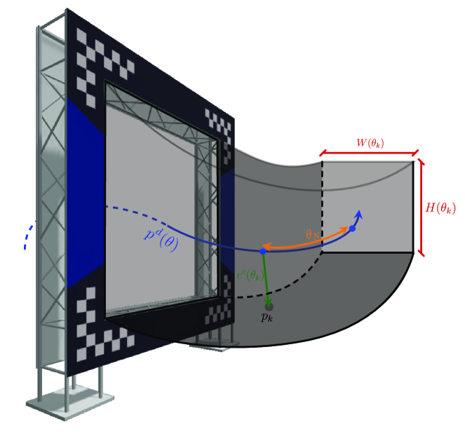
Figure 2: Safety constraints in position in the shape of a tunnel. The size of the tunnel are set exactly the same as the dimensions of the interior of the gates where at the gates and larger everywhere else.

Such a set terminal set can be for example computed by solving the following optimization problem

$$\operatorname*{argmin}_{x,u} \sum_{k=0}^{M}\|\bm{p}^{d}(\theta_{k})-\bm{p}_{k}\|_{2}^{2}$$

subject to $$\bm{x}_{0}=\bm{x}_{N}$$

$$\bm{x}_{k+1}=\bm{\hat{f}}(\bm{x}_{k},\bm{u}_{k})$$

$$\bm{x}_{k}\in\mathcal{X},\quad\bm{u}_{k}\in\mathcal{U},$$

where $M$ is the number of points that parameterize the terminal set, and the first constraints requires the trajectory to be periodic. The trajectory $\bm{p}^{d}(\theta_{k})$ is guaranteed to be positive invariant. Thanks to this terminal set, it is possible to state the following proposition.

Proposition 1

The MPCC formulation in (8) is recursively feasible and satisfies constraints at all times.

The proof follows from standard MPC recursive feasibility arguments [59]. It is possible to show that controller (8) is also inherently robust to disturbances by following the same arguments used in [60].

IV-B Dynamics augmentation

In this section we explain how to augment the nominal dynamics $\bm{f}(\bm{x},\bm{u})$ introduced in Section III-A, with a residual term $\bm{g}(\bm{x},\bm{u})$ that captures unmodeled effects.

We first provide a general overview of the forces and torques that act on the system, then identify the sources of model mismatch, and propose a set of polynomial features to approximate these terms from real world data.

We differentiate between the lift force $\bm{f}_{prop}$ produced by the propellers, and the collective aerodynamic forces $\bm{f}_{aero}$ which encompass effects such as drag, induced lift, and blade flapping. The total torque acting on the system is composed of four elements: the torque generated by the individual propellers $\bm{\tau}_{prop}$, the yaw torque $\bm{\tau}_{mot}$ arising from changes in motor speeds, the aerodynamic torque $\bm{\tau}_{aero}$ that captures a variety of aerodynamic influences, and an inertial term $\bm{\tau}_{iner}$.
While $\bm{f}_{prop}$ and $\bm{\tau}_{prop}$ can be precisely estimated from first principles, accurately modelling the aerodynamic forces is significantly more challenging. In [32], the forces acting on the individual propellers were modelled analytically using Blade Element Momentum Theory (BEM), which, due to its precision, notably raises computational demands. Instead, we adopt the methodology from [6] in which simple, low-dimensional polynomial features are fitted to real world data through conventional regression techniques. This method operates on the premise that aerodynamic effects are primarily characterized by the drone’s linear body velocity, and the average of squared (four) individual motor speeds. The features are then selected by combining the individual terms $v_{x}$, $v_{y}$, $v_{z}$, $\Omega^{2}$ in different powers:

$$f_{x} \sim v_{x}+v_{x}^{3}+\Omega^{2}+v_{x}\Omega^{2}$$

$$f_{y} \sim v_{y}+v_{y}^{3}+\Omega^{2}+v_{y}\Omega^{2}$$

$$f_{z} \sim v_{z}+v_{z}^{3}+v_{xy}+v_{xy}^{2}+v_{xy}\Omega^{2}+v_{z}\Omega^{2}+v_{xy}v_{x}\Omega^{2}$$

$$\tau_{x} \sim v_{y}+\Omega^{2}+v_{y}\Omega^{2}$$

$$\tau_{y} \sim v_{x}+\Omega^{2}+v_{x}\Omega^{2}$$

$$\tau_{z} \sim v_{x}+v_{y}.$$ (11)

The respective coefficients are identified using force and torque measurements that are directly derived onboard IMU motorspeed and IMU measurements as well as from ground truth data, captured with a VICON system. The data is gathered from the same race track to ensure that it captures the unique aerodynamic effects that arise from the racing maneuvers. It’s important to note that the coefficients are identified offline and remain constant at runtime. Additionally, the residual model requires an accurate estimate of the motor speeds, which are not provided in the original MPCC formulation from Problem 8. To address this, we modfy the initial problem to include a first-order motor model within the nominal dynamics as outlined in Eq. (1)

$$\dot{\bm{\Omega}}=\frac{1}{\tau_{mot}}(\bm{\Omega_{des}}-\bm{\Omega}),$$ (12)

where $\bm{\Omega_{des}}$ and $\bm{\Omega}$ denote the desired and the actual motor speeds, respectively.

IV-C TuRBO tuning

We consider the SMPCC controller as a black box function in the context of Bayesian Optimization. For a given set of controller parameters $\bm{\phi}$, we run an episode, collect a trajectory $\tau(\bm{\phi})$, and compute the reward $R(\tau(\bm{\phi}))$. For the sake of clarity, we will omit the trajectory from the notation and simply refer to the reward as $R(\bm{\phi})$. The controller tuning task can be framed as an optimization problem:

$$\bm{\phi}_{n+1}=\arg\max_{\bm{\phi}\in\Theta}R(\bm{\phi}).$$ (13)

Problem (13) presents two caveats: i) no analytical form of $R(\bm{\phi})$ exists, allowing only for pointwise evaluation; ii) each evaluation corresponds to completing an entire episode within the simulator, which means the number of evaluations is capped by our interaction budget with the simulated environment. BO works in an iterative manner, relying on two key ingredients: i) a probabilistic surrogate model approximating the objective function and ii) an acquisition function $\alpha(\bm{\phi})$ that determines new evaluation points, balancing exploration and exploitation. A common choice for the surrogate model are Gaussian Processes (GPs), which allow for closed-form inference of the posterior mean $\mu(\bm{\phi})$ and variance $\sigma^{2}(\bm{\phi})$. The next evaluation point $\bm{\phi}_{n+1}$ is then chosen by maximizing the acquisition function $\alpha(\bm{\phi})$. We utilize the Upper Confidence Bound (UCB) acquisition function, defined as $\alpha_{UCB}(\bm{\phi})=\mu(\bm{\phi})+\beta\sigma(\bm{\phi})$, where $\beta$ is the exploration parameter. This process is iterated until the evaluation budget is exhausted. Among the various BO methodologies, we opt for TuRBO [47], a global BO strategy that runs multiple independent local BO instances concurrently. Each local surrogate model enjoys the benefits of local BO such as diverse modeling of the objective function across different regions. Each local run explores within a Trust Region (TR) - a polytope centered around the optimal solution of the local instance. The base side length of the TR, $L$ is adjusted based on the success rate of evaluations, to guide exploration towards promising areas. In this work we use the TuRBO-1 implementation from the BOTorch library [61] and modify it for an eightfold setup, TuRBO-8.

In contrast to the baseline MPCC [14], which requires $N_{\bm{\phi}}=2n_{gates}+4$ parameters to be tuned due to the complexity of the contour function, the SMPCC reduces the number of tunable parameters to $N_{\bm{\phi}}=8$. From Problem 8, the parameters in question within the SMPCC include $Q_{l}$, $Q_{c}$, $Q_{\omega}$, $R_{v_{\theta}}$, $R_{\Delta f}$, and $\mu$, with $Q_{c}$, $Q_{\omega}$ further divided into horizontal and vertical components.

For our experiments, we define one episode of the tuning task as the completion of $M=3$ consecutive laps around the track. The reward attained at the end of the episode is calculated as the mean lap time, adjusted by a penalty factor for any solver failures:

$$R(\bm{\phi})=-\frac{1}{M}\sum_{i=0}^{M}t_{i}-\gamma r_{fail},$$ (14)

where $t_{i}$ denotes the lap time of the i-th lap, while $r_{fail}$ represents the solver failure rate, i.e. the proportion of steps that fail relative to the total steps. We apply a scaling factor of $\gamma=100$ to the penalty term. Such failures arise mainly due to infeasibilities when the system is pushed to its constraint bounds. Incorporating this penalty term has proven effective in practice, as it smoothens the objective function in favor of parameters that minimize solver failures. This reward structure is consistently applied across all experiments.

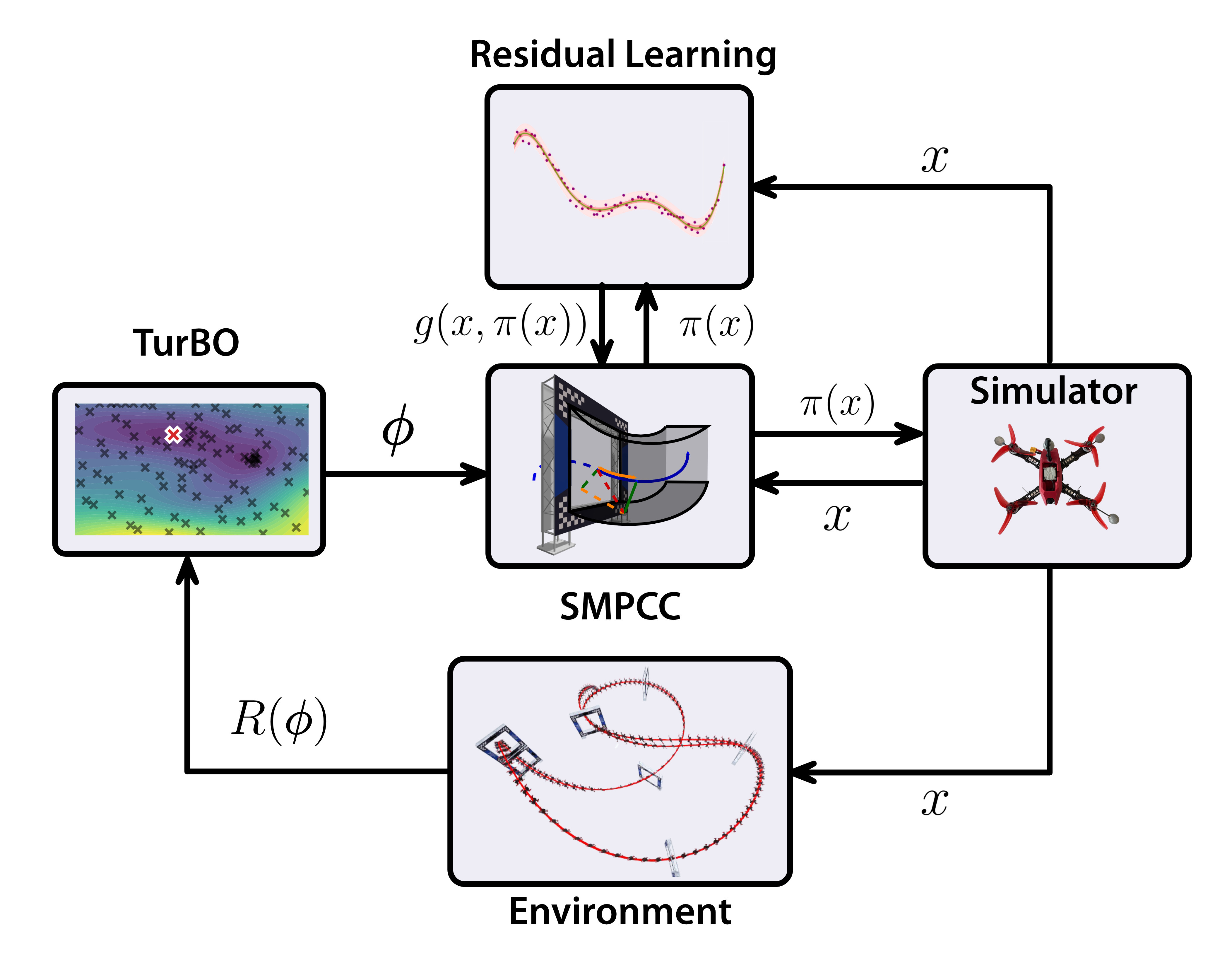
Figure 3: Overview of the complete pipeline. Starting with an initial sample of tuning parameters $\bm{\phi}$, a trajectory is run. TuRBO then receives the reward associated to the collected trajectory and then updates the tuning parameters for the next sample. For the residual model learning, data is collected from the real quadrotor system and $\bm{g}(\bm{x},\bm{u})$ is fitted to that data.

V Experiments

In this section, we compare our proposed method, SMPCC, against two baselines: RL and MPCC, and conduct a series of ablation studies. The methodology is consistent across all experiments, and utilizes the same quadrotor configuration. We choose the Split-S race track, featuring 7 gates, for all our experiments due to its prevalent use in previous works [13, 14, 15, 7]. We test the performance of our approach across three distinct simulation environments: i) a simple simulator which uses the nominal dynamics; ii) a high-fidelity simulator that calculates the propeller forces via Blade Element Momentum Theory (BEM) [32]; and iii) a data-driven simulator that predicts aerodynamic forces from real world data. We then validate our method in the real world. All experiments were executed on the same hardware under uniform conditions.

Category	Methods	Tuning	Environments
			Simple		BEM		Residual		Real World
			Lap Time [s]	SR[%]	Lap Time [s]	SR[%]	Lap Time [s]	SR[%]	Lap Time [s]	SR[%]
MPCC [14]	Nominal	WML [16]	5.38 $\pm$ 0.1	100	5.51 $\pm$ 0.06	100	5.51 $\pm$ 0.13	83.3	-	-
		TurBO	5.65 $\pm$ 1.07	89.7	5.37 $\pm$ 0.06	100	5.62 $\pm$ 0.23	96.7	5.67 $\pm$ 1.06	59.3
SMPCC (ours)	Nominal	TurBO	5.16 $\pm$ 0.02	100	5.30 $\pm$ 0.02	100	5.37 $\pm$ 0.09	100	5.41 $\pm$ 0.14	100
	w/ augment.	TurBO	5.09 $\pm$ 0.10	100	5.15 $\pm$ 0.03	100	5.19 $\pm$ 0.03	100	5.38 $\pm$ 0.26	100
	w/ random.	TurBO	5.20 $\pm$ 0.13	100	5.37 $\pm$ 0.08	100	5.26 $\pm$ 0.27	100	-	-
RL	-	-	5.14 $\pm$ 0.09	100	-	-	5.26 $\pm$ 0.32	100	5.35 $\pm$ 0.15	85.0

TABLE I: Results for MPCC, SMPCC and RL. There are four columns depending on which environment the experiment was conducted in. Three of these columns are for different simulation environments, and the last column for real world results. We can see how for our SMPCC, the success rate in all simulations and in the real world is 100%.

V-A Simulation

We train the policies across the three simulators previously described using TuRBO as the default tuning method. Each policy is allocated a total budget of 600 episodes for training, which translates to a maximum of 1800 interactions with the environment, given that each episode involves completing 3 laps. For the environment setup, simulation and training, we use a combination of Flightmare [62] and Agilicious [63] software stacks.

At test time, we select the best policy from the training phase and run 10 episodes (equivalent to 30 laps). The results reported in Table I are based on the average lap time over the 10 episodes. Additionally, we report the success rate (SR) by counting the number of episodes where the drone successfully finishes all 3 laps without any gate collisions [7]. After simulation, we select the best policy obtained in the residual simulator and deploy it in the real world. Note that while BEM and the residual simulator provide comparable accuracy levels, the latter is preferred due to its significantly lower computational demand - approximately one tenth that of the BEM simulator.

V-A1 TuRBO vs WML

We first investigate the difference between WML and TuRBO, and discuss several advantages of TuRBO. We train the baseline MPCC [14] using both variants. Despite both methods achieving comparable maximum rewards, in this section we deive into understanding how each of these explore the parameter space. In Figure 4 we illustrate two of the tuned parameters - the minimum contour weight $Q_{c}$ and the progress weight $\mu$, across the number of episodes. WML starts a new trial every 100 iterations, while TuRBO runs multiple trust regions in parallel, facilitating a broader exploration of the parameter space. This is primarily due to TuRBO’s ability to select the local instances in an informed manner, as opposed to WML’s approach of random trial restarts. An additional advantage of TuRBO is that the trust regions are independent, allowing parallel execution without incurring extra computational cost. Consequently we advocate for TuRBO as our preferred tuning algorithm, for two reasons: i) comprehensive exploration of the entire parameter space; ii) computational efficiency and scalability, which are crucial for exploring large parameter spaces.

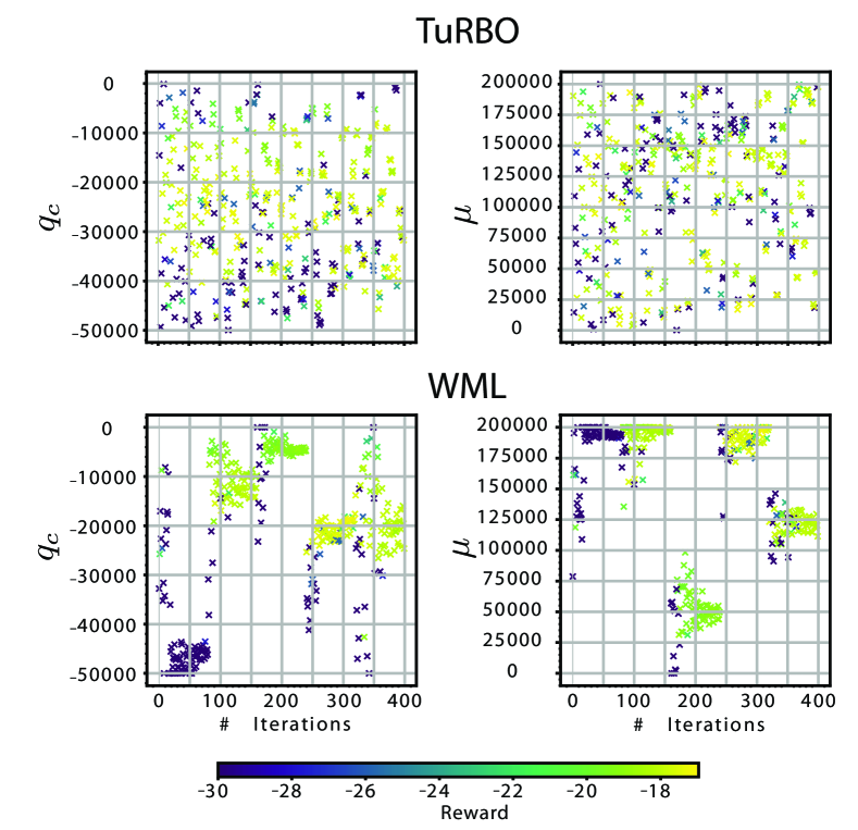
Figure 4: Parameter exploration using WML vs TuRBO. The different data samples are colored based on the collected reward. The figure shows that the WML method is prone to get stuck in local minima, while the TuRBO method is able to explore a broader parameter space.

V-A2 MPCC vs SMPCC

We train both MPCC and SMPCC using TuRBO. We make some practical adjustments to the SMPCC formulation introduced in Section IV-A. Specifically, we relax the hard constraints of the tunnel and impose soft constraints instead, which is a standard practice in MPC and can be performed in a systematic way [64]. This has several benefits: i) improves the numerical stability of the solver; ii) handles infeasibilities which arise from model mismatch by allowing minor violations; iii) maintains the low computational complexity of MPCC. This adaption does not impose any drawbacks in terms of performance/safety. The soft constraint is implemented using a barrier function $p(h(x))$ to embed the constraint into the cost function. For nonlinear constraints defined as $h(x)\geq 0$, we employ:

$$p(h(x))=\log\left(1+\exp\left(-\alpha h(x)\right)\right).$$ (15)

setting the penalty slope to $\alpha=100$. Our results, as detailed in Table I demonstrate SMPCC’s superiority over MPCC in terms of lap times and success rates. Due to spatial constraints (9), SMPCC can prevent crashes consistently without compromising the lap time. Allowing the controller to independently navigate within the tunnel, instead of following a predefined path, gives it greater flexibility to identify the best trajectory based on its current state. This strategy is akin to RL, enabling the controller to autonomously identify its optimal path, hence synthesizing the tasks of planning and control. The tunnel’s dimensions, determined by the nominal and inner gate values, $W_{n}$ and $W_{gate}$, provide a mechanism to intuitively trade off safety against performance. This balance was adjustable in test runs without necessitating re-tuning, indicating the policy’s robustness across varying tunnel widths.

In Figure 5, we show the trajectory from 10 episodes (30 laps) for both MPCC and SMPCC, noting SMPCC’s paths are notably more consistent. We attribute the inconsistency of MPCC to its representation of the contour weight as a multivariate gaussian introduces numerical asymmetry in the presence of mismatch, as the controller forcefully tries to follow the reference path, and acts poorly in the presence of disturbances.

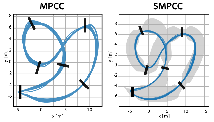
Figure 5: Simulation experiments of MPCC with the proposed SMPCC, both tuned using TuRBO

We introduce the Episode Success Rate (ESR) metric to quantify episodes completed without gate collisions. As shown in Table II, MPCC achieves an ESR of roughly 70% across all simulations, indicating that 30% of the episode evaluations are not completed successfully due to gate collisions, SMPCC approaches an ESR of nearly 100%. Failed episodes are assigned with the lowest attainable reward and do not provide valuable insights for the BO’s surrogate model updates. As such, we consider these as fruitless interactions with the environment.

Category	Methods	Tuning	Environments
			Simple	BEM	Residual
			ESR[%]	ESR[%]	ESR[%]
MPCC [14]	Nominal	WML [16]	62.9	75.7	64.4
		TurBO	69.2	70.3	53.0
SMPCC (ours)	Nominal	TurBO	99.5	100	99.8
	w/ augment.	TurBO	100	100	100
	w/ random.	TurBO	91.3	93.9	89.0

TABLE II: BO Exploration Success Rate: percentage of episodes during training which successfully complete all laps without gate collisions.

V-A3 SMPCC with Model Augmentation

Following the approach described in Section IV-B, we augment the nominal dynamics of the MPC $f(x,u)$ with a residual component $g(x.u)$. Since the residual term is a function of $v_{x}$, $v_{y}$, $v_{z}$, $\Omega^{2}$, requiring to adapt our SMPCC scheme to model the motor speeds $\Omega_{i}$, rather than the direct thrusts $f_{i}$. To this end, we model the motor dynamics as a first-order system and define the states and inputs as described in Section IV-B. In this case, increasing the number of states does not have a significant impact on the solver time in practice.

It’s also worth noting that the motor speeds are generally unavailable at runtime. We thus resort to estimating these online given the current state and applied command. These can be easily estimated from the motor model and low level betaflight controller. Note also that including the residual terms in the MPC formulation potentially introduces more numerical instability, as the features are only plausible within a specific range. To prevent this, we impose an additional constraint on the motor speeds and velocity magnitude to prevent the features from estimating beyond the range in which they characterize the dynamics accurately. We find that we are able to further reduce the lap time on all of the environments by approximately 0.1s. We attribute this improvement to a combination of the above: i) respecting the motor dynamics; ii) the actual augmentation.

V-B SMPCC with Domain Randomization

We address the robustness of the control policy against different noise realizations. The goal is to find policies which perform well amid model discrepancies. Such mismatches arise from using e.g. different hardware, leading to slight changes in mass, inertia, or thrust. We adapt the existing training pipeline to account for such noise realizations. For each iteration of the BO loop, we execute 10 different episodes each subjected to a distinct noise realization. We then collect the average reward over the 10 episodes and update the BO surrogate as usual. For fairness in comparison, we maintain the same number of interactions with the environment, which implies that the number of BO iterations is reduced by a factor 10 (from 600 to 60). In practice, reducing the number of BO iterations did not show any major limitations. We compare the obtained policies against the nominal SMPCC and observe: i) slight increase in the lap time; ii) in both cases the consistency of the trajectory is preserved; iii) 10 noise realizations are not sufficient for a truly robust policy. We conclude that the control formulation at hand is inherently robust and is able to adapt to both changes in the platform, as well as sudden changes in the dynamics. We owe this property to the controller’s replanning capability within the constraint boundaries.

V-C SMPCC vs RL

As shown in Table I, our SMPCC strategy attains lap times comparable to the leading RL policies [65]. We refer to [7], for a detailed comparison between Optimal Control vs RL. We discuss the difference between the trajectories of both in real world in Section V-D, and provide some general remarks herein. Despite both policies achieving similar performance, SMPCC ensures safety by design. We also find that it’s possible to fly with the same SMPCC policy through a variety of tracks and achieve competitive lap times without retuning, indicating good generalization, while this is generally not the case for RL policies. It’s worth noting that these advantages come at the price of more engineering efforts than an end to end learning framework. In particular, the need to account explicitely for delay compensation, solver infeasibility, adapting the MPC outputs to low level controller commands, alongside managing real-time computational solver limitations.

Figure 6: Real-world flight comparison of the MPCC controller with the Tunnel MPC (TMPC) controller proposed in this work. Even when both controllers have been tuned with TuRBO, we show that the TMPC is able to achieve faster speeds, more consistency than its MPCC counterpart and 100% success rate with no gate crashes.

V-D Real World

We test our approach in the real world with a high-performance, racing drone with a high thrust-to-weight ratio (TWR). We use the Agilicious platform [63] for the real world deployment, as detailed in [7] under the designation 4s drone. The control framework was deployed on ACADOS, using SQP_RTI for real-time computation, with the control loop runs at 100Hz. We use a horizon length of $N=20$ at a prediction rate of 25Hz, resulting in a prediction span of $T=0.8s$.

Our method runs on an offboard desktop computer equipped with an Intel(R) Core(TM) i7-8565U CPU @ 1.80GHz. A Radix FC board that contains the Betaflight firmware is used as a low level controller. This low-level controller takes as inputs body rates and collective thrusts. An RF bridge is employed to transmit commands to the drone.

For state estimation, we use a VICON system with 36 cameras that provide the platform with millimeter accuracy measurements of position and orientation at a rate of 400 Hz.

We compute the lap times and success rates as done for the simulation experiments, i.e. averaging over 10 trials (3 laps per trial). In Fig. 6 we show the comparison between the real world runs of the baseline MPCC, SMPCC (ours) and the best RL. Both MPCC and SMPCC are tuned with TuRBO. SMPCC consistently satisfies the tunnel bounds, while achieving higher speeds than the MPCC. Our policy did not crash a single time during the 10 trials, being the first approach to achieve a success rate of 100% in real world. The increase in robustness comes without a compromise in performance, as our approach achieves similar lap times to the best RL controller. SMPCC plans a trajectory very close to the edge of the gates, while in RL the deviation from the gate center is penalized in the reward, hence encouraging the drone to fly closer to the gate center. The Split-S maneuver at $x=-4.3m$, stands out as a critical test of each approach’s characteristics, as it’s performed differently in all three cases. This is the most challenging maneuver of the track and has a significant influence on the overall lap time.

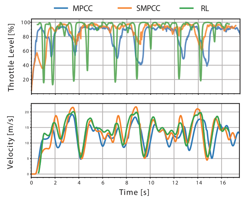
Figure 7: Real world thrust and velocity profiles for MPCC, SMPCC and RL. We note how the proposed approach is able to keep the platform extremely close to the limit of handling.

Figure 7 further explores the differences in throttle level, representing normalized commanded collective thrust, and velocity magnitude among the approaches. While velocity profiles were similar, the commanded throttle values differ significantly between the MPC approaches and RL. This is because in MPC, the solver output needs to be translated to equivalent collective thrust and desired body rate values, which are then commanded to the low level controller. This mapping is non trivial, and needs to account for delay effects. We believe that it has a significant influence on the overall performance and is a major drawback of MPC approaches. On the other hand, RL directly outputs a suitable command for the low level controller.

VI Discussion

This paper introduces SMPCC, a Safe MPCC controller for drone racing that prevents collisions against the gates. We augment the nominal dynamics of the controller with a residual term that is obtained from real-world data and captures unmodeled behaviors such as aerodynamic effects and propeller forces. We tune the controller parameters using TuRBO, a state-of-the-art Bayesian optimization algorithm that efficiently compromises between local and global exploration. Our approach addresses several of the limitations encountered in the baseline MPCC [14]: i) robustness against gate collisions; ii) suboptimality from following a predefined optimal trajectory; iii) tuning effort incurred from tuning a high dimensional parameter space. We benchmark our approach against the baseline MPCC and the best-performing RL controller in both simulation and real-world experiments and show that we are on par in terms of lap times while attaining safety against collisions. Our approach is the first to achieve 100% success rate in real-world experiments.

Nonetheless, SMPCC also presents several limitations. First, there is a need for a centerline that passes through the gate centers and is used as the basis to construct the safety set. While there is no computational effort incurred from it, as it can be almost any smooth spline, it does require some manual effort to be determined. Additionally, unlike RL architectures, our approach restricts the platform to operate within a predefined safety set. This limitation hinders its ability to freely explore and develop new behaviors necessary for executing complex maneuvers, such as loops or ladders, which are commonly seen in drone racing environments.

It remains for future work to understand how the choice of the centerline influences the solution and find a method that generalizes to all track configurations. Second, our approach takes significantly longer to train than RL, as the environment cannot be parallelized on the GPU. This is because the solver calls cannot be batched into tensor operations, as done with MLP based policies. Third, the performance of our controller is limited at run time as it requires an optimization problem to be solved at each step, whereas RL methods require a simple forward pass of the neural network.

Thus, we conclude that the main advantage of our approach is that it provides an intuitive lever to trade-off between performance and robustness. By shrinking the width of the tunnel, the quadrotor flies safely through the track. We can then gradually adjust the width to increase performance. Adjustments in the tunnel width can be made directly without further fine-tuning.

VII Acknowledgments

This work was supported by the European Union’s Horizon Europe Research and Innovation Programme under grant agreement No. 101120732 (AUTOASSESS) and the European Research Council (ERC) under grant agreement No. 864042 (AGILEFLIGHT). The authors especially thank Amon Lahr for his helpful acados tips, and Jiaxu Xing and Ismail Geles for their help with the experiments.

References

- [1] G. Loianno and D. Scaramuzza, “Special issue on future challenges and opportunities in vision-based drone navigation,” 2020.
- [2] S. Rajendran and S. Srinivas, “Air taxi service for urban mobility: a critical review of recent developments, future challenges, and opportunities,” Transportation Research Part E-logistics and Transportation Review, Nov 2020.
- [3] H. Shakhatreh, A. H. Sawalmeh, A. Al-Fuqaha, Z. Dou, E. Almaita, I. Khalil, N. S. Othman, A. Khreishah, and M. Guizani, “Unmanned aerial vehicles (uavs): A survey on civil applications and key research challenges,” Ieee Access, vol. 7, pp. 48572–48634, 2019.
- [4] J. Betz, H. Zheng, A. Liniger, U. Rosolia, P. Karle, M. Behl, V. Krovi, and R. Mangharam, “Autonomous vehicles on the edge: A survey on autonomous vehicle racing,” IEEE Open Journal of Intelligent Transportation Systems, vol. 3, pp. 458–488, 2022.
- [5] D. Hanover, A. Loquercio, L. Bauersfeld, A. Romero, R. Penicka, Y. Song, G. Cioffi, E. Kaufmann, and D. Scaramuzza, “Autonomous drone racing: A survey,” arXiv e-prints, pp. arXiv–2301, 2023.
- [6] E. Kaufmann, L. Bauersfeld, A. Loquercio, M. Müller, V. Koltun, and D. Scaramuzza, “Champion-level drone racing using deep reinforcement learning,” Nature, vol. 620, pp. 982–987, Aug 2023.
- [7] Y. Song, A. Romero, M. Mueller, V. Koltun, and D. Scaramuzza, “Reaching the limit in autonomous racing: Optimal control versus reinforcement learning,” Science Robotics, p. adg1462, 2023.
- [8] S. Gu, L. Yang, Y. Du, G. Chen, F. Walter, J. Wang, Y. Yang, and A. Knoll, “A review of safe reinforcement learning: Methods, theory and applications,” arXiv preprint arXiv:2205.10330, 2022.
- [9] L. Brunke, M. Greeff, A. W. Hall, Z. Yuan, S. Zhou, J. Panerati, and A. P. Schoellig, “Safe learning in robotics: From learning-based control to safe reinforcement learning,” Annual Review of Control, Robotics, and Autonomous Systems, vol. 5, pp. 411–444, 2022.
- [10] K. P. Wabersich and M. N. Zeilinger, “A predictive safety filter for learning-based control of constrained nonlinear dynamical systems,” Automatica, vol. 129, p. 109597, 2021.
- [11] H. Dai, B. Landry, L. Yang, M. Pavone, and R. Tedrake, “Lyapunov-stable neural-network control,” in Proceedings of Robotics: Science and Systems, July 2021.
- [12] A. Romero, Y. Song, and D. Scaramuzza, “Actor-critic model predictive control,” in 2024 IEEE International Conference on Robotics and Automation (ICRA).
- [13] P. Foehn, A. Romero, and D. Scaramuzza, “Time-optimal planning for quadrotor waypoint flight,” Science Robotics, vol. 6, no. 56, 2021.
- [14] A. Romero, S. Sun, P. Foehn, and D. Scaramuzza, “Model predictive contouring control for time-optimal quadrotor flight,” IEEE Transactions on Robotics, pp. 1–17, 2022.
- [15] A. Romero, R. Penicka, and D. Scaramuzza, “Time-optimal online replanning for agile quadrotor flight,” IEEE Robotics and Automation Letters, vol. 7, no. 3, pp. 7730–7737, 2022.
- [16] A. Romero, S. Govil, G. Yilmaz, Y. Song, and D. Scaramuzza, “Weighted maximum likelihood for controller tuning,” in 2023 IEEE International Conference on Robotics and Automation (ICRA), pp. 1334–1341, IEEE, 2023.
- [17] L. P. Fröhlich, C. Küttel, E. Arcari, L. Hewing, M. N. Zeilinger, and A. Carron, “Model learning and contextual controller tuning for autonomous racing,” arXiv preprint arXiv:2110.02710, 2021.
- [18] A. Majumdar and R. Tedrake, “Funnel libraries for real-time robust feedback motion planning,” The International Journal of Robotics Research, vol. 36, no. 8, pp. 947–982, 2017.
- [19] J. Ji, X. Zhou, C. Xu, and F. Gao, “Cmpcc: Corridor-based model predictive contouring control for aggressive drone flight,” in Experimental Robotics: The 17th International Symposium, pp. 37–46, Springer, 2021.
- [20] J. Arrizabalaga and M. Ryll, “Towards time-optimal tunnel-following for quadrotors,” in 2022 International Conference on Robotics and Automation (ICRA), pp. 4044–4050, IEEE, 2022.
- [21] M. Mueller, S. Lupashin, and R. D’Andrea, “Quadrocopter ball juggling,” pp. 4972–4978, 2011.
- [22] R. Mahony, V. Kumar, and P. Corke, “Multirotor aerial vehicles: Modeling, estimation, and control of quadrotor,” vol. 19, no. 3, pp. 20–32, 2012.
- [23] D. Mellinger, N. Michael, and V. Kumar, “Trajectory generation and control for precise aggressive maneuvers with quadrotors,” vol. 31, no. 5, pp. 664–674, 2012.
- [24] M. W. Mueller, M. Hehn, and R. D’Andrea, “A computationally efficient algorithm for state-to-state quadrocopter trajectory generation and feasibility verification,” 2013.
- [25] C. Qin, M. S. Michet, J. Chen, and H. H.-T. Liu, “Time-optimal gate-traversing planner for autonomous drone racing,” arXiv preprint arXiv:2309.06837, 2023.
- [26] A. Loquercio, E. Kaufmann, R. Ranftl, A. Dosovitskiy, V. Koltun, and D. Scaramuzza, “Deep drone racing: From simulation to reality with domain randomization,” IEEE Trans. Robotics, vol. 36, no. 1, pp. 1–14, 2019.
- [27] E. Kaufmann, L. Bauersfeld, and D. Scaramuzza, “A benchmark comparison of learned control policies for agile quadrotor flight,” in 2022 International Conference on Robotics and Automation (ICRA), IEEE, 2022.
- [28] L. O. Rojas-Perez and J. Martinez-Carranza, “Deeppilot: A CNN for autonomous drone racing,” Sensors, vol. 20, no. 16, p. 4524, 2020.
- [29] J. Hwangbo, I. Sa, R. Siegwart, and M. Hutter, “Control of a quadrotor with reinforcement learning,” IEEE Robotics and Automation Letters, vol. 2, no. 4, pp. 2096–2103, 2017.
- [30] W. Koch, R. Mancuso, R. West, and A. Bestavros, “Reinforcement learning for uav attitude control,” ACM Transactions on Cyber-Physical Systems, vol. 3, no. 2, pp. 1–21, 2019.
- [31] N. O. Lambert, D. S. Drew, J. Yaconelli, S. Levine, R. Calandra, and K. S. Pister, “Low-level control of a quadrotor with deep model-based reinforcement learning,” IEEE Robotics and Automation Letters, vol. 4, no. 4, pp. 4224–4230, 2019.
- [32] L. Bauersfeld, E. Kaufmann, P. Foehn, S. Sun, and D. Scaramuzza, “Neurobem: Hybrid aerodynamic quadrotor model,” in Proceedings of Robotics: Science and Systems, 2021.
- [33] Y. Song, M. Steinweg, E. Kaufmann, and D. Scaramuzza, “Autonomous drone racing with deep reinforcement learning,” in 2021 IEEE/RSJ International Conference on Intelligent Robots and Systems (IROS), pp. 1205–1212, IEEE, 2021.
- [34] K. J. Åström, “Theory and applications of adaptive control—a survey,” automatica, vol. 19, no. 5, pp. 471–486, 1983.
- [35] M. J. Grimble, “Implicit and explicit lqg self-tuning controllers,” IFAC Proceedings Volumes, vol. 17, no. 2, pp. 941–947, 1984.
- [36] K. J. Åström, T. Hägglund, C. C. Hang, and W. K. Ho, “Automatic tuning and adaptation for pid controllers-a survey,” Control Engineering Practice, vol. 1, no. 4, pp. 699–714, 1993.
- [37] M. A. Mohd Basri, A. R. Husain, and K. A. Danapalasingam, “Intelligent adaptive backstepping control for mimo uncertain non-linear quadrotor helicopter systems,” Transactions of the Institute of Measurement and Control, vol. 37, no. 3, pp. 345–361, 2015.
- [38] A. Schperberg, S. Di Cairano, and M. Menner, “Auto-tuning of controller and online trajectory planner for legged robots,” IEEE Robotics and Automation Letters, vol. 7, no. 3, pp. 7802–7809, 2022.
- [39] M. Zanon and S. Gros, “Safe reinforcement learning using robust mpc,” IEEE Transactions on Automatic Control, vol. 66, no. 8, pp. 3638–3652, 2020.
- [40] S. Cheng, M. Kim, L. Song, C. Yang, Y. Jin, S. Wang, and N. Hovakimyan, “Difftune: Auto-tuning through auto-differentiation,” arXiv preprint arXiv:2209.10021, 2022.
- [41] J. De Schutter, M. Zanon, and M. Diehl, “Tunempc—a tool for economic tuning of tracking (n)mpc problems,” IEEE Control Systems Letters, vol. 4, no. 4, pp. 910–915, 2020.
- [42] A. Loquercio, A. Saviolo, and D. Scaramuzza, “Autotune: Controller tuning for high-speed flight,” IEEE Robotics and Automation Letters, vol. 7, no. 2, pp. 4432–4439, 2022.
- [43] W. Edwards, G. Tang, G. Mamakoukas, T. Murphey, and K. Hauser, “Automatic tuning for data-driven model predictive control,” in 2021 IEEE International Conference on Robotics and Automation (ICRA), pp. 7379–7385, IEEE, 2021.
- [44] M. Menner and M. N. Zeilinger, “Maximum likelihood methods for inverse learning of optimal controllers,” IFAC-PapersOnLine, vol. 53, no. 2, pp. 5266–5272, 2020.
- [45] F. Berkenkamp, A. P. Schoellig, and A. Krause, “Safe controller optimization for quadrotors with gaussian processes,” in 2016 IEEE International Conference on Robotics and Automation (ICRA), pp. 491–496, IEEE, 2016.
- [46] A. Marco, P. Hennig, J. Bohg, S. Schaal, and S. Trimpe, “Automatic lqr tuning based on gaussian process global optimization,” in 2016 IEEE international conference on robotics and automation (ICRA), pp. 270–277, IEEE, 2016.
- [47] D. Eriksson, M. Pearce, J. Gardner, R. D. Turner, and M. Poloczek, “Scalable global optimization via local Bayesian optimization,” in Advances in Neural Information Processing Systems, pp. 5496–5507, 2019.
- [48] N. A. Spielberg, M. Brown, and J. C. Gerdes, “Neural network model predictive motion control applied to automated driving with unknown friction,” IEEE Transactions on Control Systems Technology, vol. 30, no. 5, pp. 1934–1945, 2021.
- [49] K. Y. Chee, T. Z. Jiahao, and M. A. Hsieh, “Knode-mpc: A knowledge-based data-driven predictive control framework for aerial robots,” IEEE Robotics and Automation Letters, vol. 7, no. 2, pp. 2819–2826, 2022.
- [50] A. Saviolo, G. Li, and G. Loianno, “Physics-inspired temporal learning of quadrotor dynamics for accurate model predictive trajectory tracking,” IEEE Robotics and Automation Letters, vol. 7, no. 4, pp. 10256–10263, 2022.
- [51] G. Williams, P. Drews, B. Goldfain, J. M. Rehg, and E. A. Theodorou, “Information-theoretic model predictive control: Theory and applications to autonomous driving,” IEEE Transactions on Robotics, vol. 34, no. 6, pp. 1603–1622, 2018.
- [52] C. J. Ostafew, A. P. Schoellig, and T. D. Barfoot, “Robust constrained learning-based nmpc enabling reliable mobile robot path tracking,” The International Journal of Robotics Research, vol. 35, no. 13, pp. 1547–1563, 2016.
- [53] U. Rosolia and F. Borrelli, “Learning how to autonomously race a car: a predictive control approach,” IEEE Transactions on Control Systems Technology, vol. 28, no. 6, pp. 2713–2719, 2019.
- [54] G. Torrente, E. Kaufmann, P. Föhn, and D. Scaramuzza, “Data-driven mpc for quadrotors,” IEEE Robotics and Automation Letters, vol. 6, no. 2, pp. 3769–3776, 2021.
- [55] M. Mehndiratta, E. Camci, and E. Kayacan, “Automated tuning of nonlinear model predictive controller by reinforcement learning,” in 2018 IEEE/RSJ International Conference on Intelligent Robots and Systems (IROS), pp. 3016–3021, IEEE, 2018.
- [56] A. Carron, E. Arcari, M. Wermelinger, L. Hewing, M. Hutter, and M. N. Zeilinger, “Data-driven model predictive control for trajectory tracking with a robotic arm,” IEEE Robotics and Automation Letters, vol. 4, no. 4, pp. 3758–3765, 2019.
- [57] G. Williams, N. Wagener, B. Goldfain, P. Drews, J. M. Rehg, B. Boots, and E. A. Theodorou, “Information theoretic mpc for model-based reinforcement learning,” in 2017 IEEE International Conference on Robotics and Automation (ICRA), pp. 1714–1721, IEEE, 2017.
- [58] A. Lahr, A. Zanelli, A. Carron, and M. N. Zeilinger, “Zero-order optimization for gaussian process-based model predictive control,” European Journal of Control, vol. 74, p. 100862, 2023.
- [59] J. Rawlings, D. Mayne, and M. Diehl, Model Predictive Control: Theory, Computation, and Design. Nob Hill Publishing.
- [60] L. Numerow, A. Zanelli, A. Carron, and M. N. Zeilinger, “Inherently robust suboptimal mpc for autonomous racing with anytime feasible sqp,” 2024.
- [61] M. Balandat, B. Karrer, D. R. Jiang, S. Daulton, B. Letham, A. G. Wilson, and E. Bakshy, “BoTorch: A Framework for Efficient Monte-Carlo Bayesian Optimization,” in Advances in Neural Information Processing Systems 33, 2020.
- [62] Y. Song, S. Naji, E. Kaufmann, A. Loquercio, and D. Scaramuzza, “Flightmare: A flexible quadrotor simulator,” in Conference on Robot Learning, 2020.
- [63] P. Foehn, E. Kaufmann, A. Romero, R. Penicka, S. Sun, L. Bauersfeld, T. Laengle, G. Cioffi, Y. Song, A. Loquercio, and D. Scaramuzza, “Agilicious: Open-source and open-hardware agile quadrotor for vision-based flight,” Science Robotics, vol. 7, no. 67, 2022.
- [64] K. P. Wabersich and M. N. Zeilinger, “Predictive control barrier functions: Enhanced safety mechanisms for learning-based control,” IEEE Transactions on Automatic Control, vol. 68, no. 5, pp. 2638–2651, 2023.
- [65] Y. Song, M. Steinweg, E. Kaufmann, and D. Scaramuzza, “Autonomous drone racing with deep reinforcement learning,” in 2021 IEEE/RSJ International Conference on Intelligent Robots and Systems (IROS), pp. 1205–1212, 2021.