DeepMIF: Deep Monotonic Implicit Fields
for Large-Scale LiDAR 3D Mapping

Abstract

Recently, significant progress has been achieved in sensing real large-scale outdoor 3D environments, particularly by using modern acquisition equipment such as LiDAR sensors. Unfortunately, they are fundamentally limited in their ability to produce dense, complete 3D scenes. To address this issue, recent learning-based methods integrate neural implicit representations and optimizable feature grids to approximate surfaces of 3D scenes. However, naively fitting samples along raw LiDAR rays leads to noisy 3D mapping results due to the nature of sparse, conflicting LiDAR measurements. Instead, in this work we depart from fitting LiDAR data exactly, instead letting the network optimize a non-metric monotonic implicit field defined in 3D space. To fit our field, we design a learning system integrating a monotonicity loss that enables optimizing neural monotonic fields and leverages recent progress in large-scale 3D mapping. Our algorithm achieves high-quality dense 3D mapping performance as captured by multiple quantitative and perceptual measures and visual results obtained for Mai City, Newer College, and KITTI benchmarks. The code of our approach will be made publicly available.

I Introduction

Implicit 3D representations, i.e. algorithms that represent shapes and scenes via level-sets of functions (fields) obtained by approximating sensor 3D measurements, enjoy well-deserved popularity for scene modeling. Their core advantages compared to other types of 3D representations (e.g., point sets or volumetric grid) include their ability to accurately model shapes and scenes of arbitrary topology and resolution at moderate computational cost. Supported by the progress for deep neural networks that offer easy fusion of multi-modal data, recently proposed neural implicit surfaces can now be optimized from acquisitions in the form of 3D samples [1, 2], RGB images [3], or RGB-D sequences [4, 5]. As a result, neural implicit fields are starting to see interest in the robotics domain where they are explored for large-scale 3D mapping [6, 7, 8, 9], odometry estimation [10], and localization [11] applications.

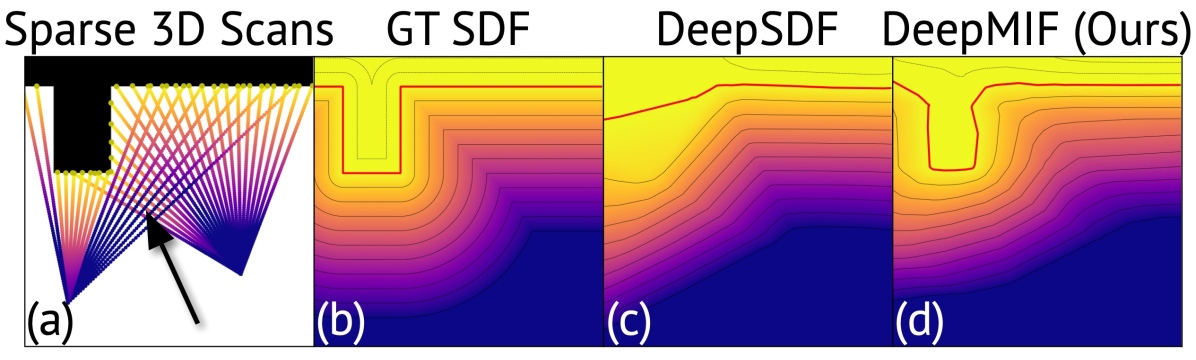
Figure 1: LiDAR 3D scans (a) generate view-inconsistent range data (pointed to by arrow) rather than projective SDF (b). Direct optimization supervised by oblique rather than projective distances [1] does not account for this effect, resulting in loss of surface features (c); in contrast, learning our implicit function (d) is able to preserve higher detail. Red line corresponds to zero level set.

Directly extending these methods to large outdoor 3D environments typical for mobile robotics (e.g., autonomous driving) which is the focus of this work, however, is challenging. Commonly, neural implicit models are optimized for exhaustively sampled 3D scenes and rely on accurate, consistent distance-to-surface measurements; depth cameras used in many indoor scenarios to some degree satisfy these assumptions [5]. However, a commonly used sensing setup in outdoor robotics consists of one or many RGB cameras and rotating LiDAR scanners. Not only do their acquisitions generate a sparse and noisy supervision signal, but can be also possibly conflicting at the same 3D point due to difference in incident angles of rays emitted in two scanning locations [10] (see Fig. 1). Recognizing these limitations, recent methods proposed to process such multi-scan data by involving normals [10, 8]; however, normals estimation can be very unstable if done on noisy 3D samples.

Motivated by these challenges, in this paper we address the case where noisy, inconsistent laser range scans are used for neural implicit surface fitting. To this end, we propose monotonic implicit functions (MIF), a scene representation suitable for addressing the challenges pertaining to the lack of the accurate ground-truth such as signed distance field (SDF). Instead of requiring that an exact SDF is produced by the LiDAR sensor, we find a non-increasing (along each emitted ray) field whose zero level-set coincides with that of the true SDF, thus bypassing the need for accurate distance-to-surface values during training, but still allowing accurate surface extraction. To fit our field given the sensor data, we design a learning system for optimizing monotonic functions (using monotonicity loss) within a framework for fitting neural implicits integrating a hierarchical latent feature grid and adaptive point sampling. As a result, our approach is capable of performing reconstruction of large-scale 3D LiDAR acquisitions using optimization, without any ground-truth data other than the 3D scan itself.

We evaluate our approach against five methods: based on depth fusion [12], interpolation [13], completion [14], and recent learning-based implicit reconstruction approaches [6, 10]. We summarize our contributions as follows:

• We propose an alternative implicit surface representation, monotonic implicit field, for large-scale 3D mapping with LiDAR point clouds.

• We demonstrate an implementation of our implicit field within a large-scale 3D mapping system that achieves improved surface reconstruction performance on multiple challenging benchmarks.

II Related Work

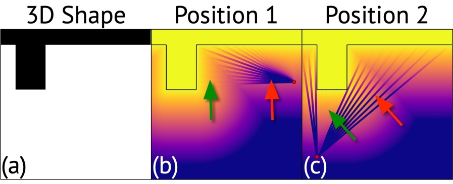
Figure 2: LiDAR scanners generate oblique distances (distance along the ray, color of foreground lines) deviating from projective distances ((b)–(c), background color). Depending on scanner position (red dots) and scanning angles, these quantities can be either slightly (areas pointed by green arrows) or significantly (areas pointed by red arrows) different.

3D reconstruction from scanned data has been explored for decades and keeps being researched; for a broader perspective, we refer the reader to the surveys on 3D reconstruction [15], RGB-D mapping [16], and neural fields [17]. Mapping large 3D environments acquired by range scanners or LiDARs has been approached from a variety of perspectives. To achieve smooth, continuous and coherent surfaces implicit surface representations such as surfels [18], volumetric truncated signed distance function (TSDF)  [19, 20], implicit representation meshes [21] are being actively employed into reconstruction approaches. TSDF has advanced among other approaches to achieve more continuous representation of 3D scenes, allowing for better interpolation, fusion from multiple viewpoints, and robustness to noise and topological changes.

TSDF fusion, starting with a classical approach [19], performs integration of a set of posed range-images into a coherent volumetric TSDF; memory requirements of the original method scale linearly with the size of the output map. To extend TSDF fusion to large-scale 3D mapping such as outdoor LiDAR scans, its recent variants incorporate advanced spatial data structures such as hash tables [22], octrees [23, 24, 25], and VDB [12]. In many instances, these methods provide robust reconstruction results, yet they may struggle to complete geometry in under-sampled areas as they lack strong geometric priors. To address the issue, recent scene completion approaches [26, 14] seek to predict occluded geometry in a self-supervised loop, going from incomplete to more complete fused reconstructions [19, 12]. Multiple methods explore combining volumetric occupancy and semantics for semantic scene completion (SSC) [27, 28, 29, 30, 31] but require semantic annotations during training. Unlike our approach, all these methods remain limited in their spatial resolution, high though it may be. We compare our method to recent volumetric VDB-based TSDF fusion [12] and learned completion [14].

Poisson Surface Reconstruction (PSR) [32, 33] is a seminal approach to implicit surface reconstruction from dense point clouds based on a local smoothness prior. PUMA [13] extends PSR to offline mapping with sparse LiDAR 3D scans; we compare against this method in our evaluation.

Multiple recent learning-based methods can train effective reconstruction priors from shape datasets. To model single shapes that are commonly assumed to be closed and watertight, pioneering approaches fit collections of latent codes and decoder networks to point datasets, predicting signed distance functions (SDFs) [1] and occupancy functions (OFs) [2]. Other types of target objects may require choosing a different implicit representation; e.g., for open surfaces such as garments, sign-agnostic [34] or unsigned [35, 36, 37] representations prove more effective than SDFs. Objects with internal structures benefit from fitting generalised representations [38] descibing spatial relationships between any two points, rather than a point and a surface. Due to their limited capacity, these methods cannot fit complex scenes with satisfactory accuracy.

Scaling neural implicit functions to large scenes can be achieved by introducing a collection of spatially latent codes instead of a single latent code. In this direction, dense volumetric feature grids are the simplest option [39, 40, 41], yet again scale linearly with scene complexity. To optimize memory use and speed up mapping, several recent approaches define and optimize a multi-resolution feature grid [42, 43, 44]. Multi-resolution latent hierarchies have been developed for LiDAR 3D mapping [6, 8, 11, 7]; among these, we compare to a representative LiDAR-based neural mapping method [6].

Most recently, building on the success of neural radiance fields [45] and neural implicit surfaces [3], several methods adopted volumetric rendering to serve for optimizing the latent grid [4, 5, 10, 9]. We compare our method to such an approach targeting LiDAR acquisitions [10].

III Method

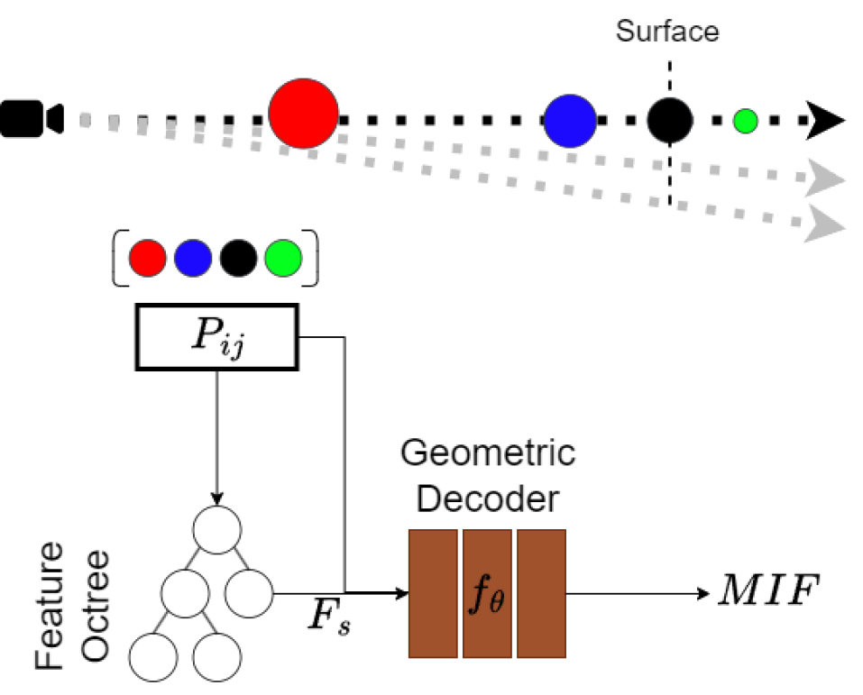
Figure 3: Our algorithm comprises three main components: a sampling strategy, a feature octree, and an MLP decoder. For visualization purposes, each point is colored based on its input order and sized by its signed distance to the surface. Monotonicity loss is enforced according to this coloring order.

III-A Method Overview

Our algorithm accepts as input a set of posed 3D LiDAR scans $\{(P_{i},T_{i}^{L})\}_{i=1}$, where 4$\times$4 pose $T_{i}^{L}$ corresponds to LiDAR location. As output, it produces a 3D reconstruction of the scene in the form of a triangle mesh extracted from an (unknown) implicit field $f$ satisfying general conditions outlined in Section III-A. We approximate the field by a neural network $f_{\theta}$ (Section III-C) designing it similarly to existing neural implicit fields [1, 39]; specifically, our implicit network accepts a feature vector $z\in\mathbb{R}^{n}$ and a 3D location $p\in\mathbb{R}^{3}$, and generates a value $y\in\mathbb{R}$ of a volumetric function via $y=f_{\theta}(p;z)$. To learn our neural field on the given data, we optimize a set of 3D losses imposed on our approximator $f_{\theta}$. Finally, we implement routines to support training our system in a variety of settings and datasets (Section III-D). A high-level illustration of our pipeline is presented in Figure 3.

III-B Monotonic Implicit Scene Representation

Neural Implicits and Level Sets

Scenes can be represented by prescribing a scalar value (e.g., signed distance-to-surface [1] or binary occupancy [2]), $s\in\mathbb{R}$, to each 3D point sample $\bm{x}\in\mathbb{R}^{3}$; then, an implicit function $f(\bm{x}):\mathbb{R}^{3}\to\mathbb{R}$ is said to describe the surface $\mathcal{S}$ of the scene. For instance, a (projective) signed distance function (SDF) maps 3D points to their closest projections on the (closed) surface via

$$f_{\text{SDF}}(\bm{x})=(-1)^{\chi_{\mathcal{V}}(\bm{x})}\cdot\arg\min\limits_{\bm{p}\in\mathcal{S}}||\bm{x}-\bm{p}||$$ (1)

where $\mathcal{V}$ is the volume enclosed by $\mathcal{S}$ and $\chi_{\mathcal{V}}(\bm{x})$ its membership function. To extract the surface of the scene explicitly (e.g., in the form of a triangle mesh), one computes a level-set $\{\bm{x}:f(\bm{x})=s_{0}\}$ of $f$ at a certain level $s_{0}$ such as zero.

Implicit fields such as SDFs can be represented by neural nets [1]; shape collections (or spatially large scenes [40]) can be encoded by parameterizing (conditioning) a learned implicit function $f_{\theta}(\bm{x};\bm{z})$ with a multivariate latent variable $\bm{z}\in\mathbb{R}^{d}$ whose values are optimized jointly with $f_{\theta}$.

Our Implicit Representation

Assuming that true values of the sought SDF in (1) can be sampled at any given 3D point, conventional methods [1, 40] sample points exhaustively near surfaces to optimize approximator parameters $\theta$ and a collection of latent shape codes $\{z_{i}\}$. For LiDAR 3D scans, SDF values are unknown for most 3D locations apart from a sparse set of points sampled along rays connecting scanned 3D points $\{\bm{p}_{i}\}$ and scanner locations. Specifically, if $\bm{o}$ is the sensor location and $\bm{q}(t)=\bm{o}+t\bm{d}_{i}$ is a laser ray emitted from the sensor in the direction $\bm{d}_{i}$ towards point $\bm{p}_{i}$, then the distance $f_{\text{ray}}(\bm{q})=||\bm{q}-\bm{p}_{i}||$ encodes proximity to the surface. However, treating such values as projective distances (in the sense of Eq. 1) is incorrect as LiDAR rays are not orthogonal to surfaces; instead, $f_{\text{ray}}(\bm{q})$ encodes oblique distances that significantly deviate from projective ones (e.g., at low incidence angles) and vary across sensor positions (see Fig. 2). As a result, using oblique SDFs directly for learning yields imprecise, contradictory training signal if used with multiple aligned LiDAR scans, leading to blurry, incomplete reconstructions (Fig. 1).

To circumvent the flaws of oblique SDFs, multiple methods transform them into occupancy probabilities by a sigmoid function (SHINE [6]), or project them along estimated surface normals (NeRF-LOAM [10] and N${}^{\text{3}}$-Mapping [8]) or along gradients of neural approximators (LocNDF [11]). These methods enjoy initial success, but are still not free from limitations as neither of them compensates for non-projective distances completely. Estimating normals from sparse, noisy point clouds is known to be an unstable operation (see, e.g., [46]).

In this work, we adopt a different approach and let the network optimize a surface-aware implicit field without fitting all sampled SDF values directly. Instead, we consider a more general implicit field whose values are

1. zero at surface locations (i.e., lidar readings);

2. positive outside and negative inside the shape;

3. monotonically non-increasing along each cast ray.

We refer to our implicit function as monotonic implicit field (MIF). While conditions (a) and (b) are standard for implicit functions including SDFs and occupancy maps [1, 2], (c) aims to relax the requirement of precisely matching conflicting values of oblique distances corresponding to different scans. While exceptions to this assumption may occur (particularly, for rays passing near but outside shapes), we consider it to be more realistic compared to the assumption of correct SDF values. Hence, a wider range of non-metric implicit fields consistent with LiDAR data can be obtained (Fig. 1). Our MIF can be meshed (e.g., by marching cubes [47]) as a usual implicit function to obtain a surface.

III-C Neural Architecture for 3D Mapping

	Mai City						Newer College
Method	$\acc\downarrow$	$\comp\downarrow$	$\cd\downarrow$	$\pre\uparrow$	$\rec\uparrow$	$\fscore\uparrow$	$\acc\downarrow$	$\comp\downarrow$	$\cd\downarrow$	$\pre\uparrow$	$\rec\uparrow$	$\fscore\uparrow$
Make-It-Dense	0.0407	0.6421	0.6494	95.0721	36.2370	52.4735	0.1615	0.3112	0.4773	48.1863	44.0248	46.0116
VDBFusion	0.1834	0.5378	0.8356	75.8177	33.9370	46.8868	0.9161	0.1018	1.7124	39.5705	73.9181	51.5466
NeRF-LOAM	0.1684	0.5509	1.0494	97.8249	33.1076	49.4720	0.6369	0.1100	1.3055	64.2951	69.1659	66.6416
PuMa	0.4104	0.5280	1.4722	72.1234	35.2944	47.3954	0.2429	0.3027	0.5749	38.4452	41.3618	39.8502
SHINE-Mapping	0.2983	0.5337	1.3583	87.4361	37.1117	52.1069	0.7191	0.0995	1.4062	66.3215	74.9309	70.3639
Ours	0.1360	0.5335	0.7558	94.6374	38.4505	54.6835	0.7123	0.0987	1.5758	63.5637	77.7812	69.9574

TABLE I: Quantitative comparison of reconstruction quality on Mai City [13] and Newer College [48] benchmarks. The best performing method is denoted in bold, and the second-best in italics.

Query Point Sampling

Let $P_{i}=\{(\bm{p}_{ij},\tau_{ij})\}$ be a point cloud acquired by a sensor emitting rays in directions $\{\bm{d}_{ij}\}$ from $\bm{o}_{i}$, where $\tau_{ij}=||\bm{p}_{ij}-\bm{o}_{i}||$ refers to the acquired depth. To produce training point instances, we sample points according to the relation $\bm{p}^{\text{tr}}_{ij}(t)=\bm{o}_{i}+t\bm{d}_{ij}$ by selecting values of the parameter $t$. Specifically, we sample $M_{f}$, $M_{s}$ and $M_{o}$ values of $t$ from segments $[\tau_{ij}-\gamma-\varepsilon,\tau_{ij}-\varepsilon]$, $[\tau_{ij}-\varepsilon,\tau_{ij}+\varepsilon]$, and $[\tau_{ij}+\varepsilon,\tau_{ij}+\varepsilon+\theta]$ respectively. For training, we record pairs $(\bm{p}_{ij,m},r_{ij,m})$ of point coordinates and signed distances $r_{ij,m}=\tau_{ij,m}-t_{ij}$ to the original readings, and collect the original sets $P_{i}$ and sampled data into our final training set $P$. Within each ray, generated points are sorted w.r.t. their values of $t$ and serve for direct supervision of our implicit function. Samples within $\varepsilon$ to sensor readings are used for building the feature octree.

Hierarchical Feature Octree

Our approach, similarly to existing frameworks [1, 39], jointly optimizes network parameters and local latent codes associated with sampled points during training. More specifically, we take inspiration from SHINE [6] and assign latent codes to leaf nodes of a multi-resolution hierarchical octree constructed on top of the input point cloud. Constructing a local latent code with the octree hierarchy involves querying eight nodes from last $H$ level of the octree hierarchy, trilinearly interpolating them to form level-specific codes, and fusing level-specific codes into the aggregated latent code through summation. For constant-time queries, we convert points into locality-preserving spatial hashes (Morton codes) and query hash tables constructed for each level in the octree [6]. The point coordinates and its latent code are fed into the decoder network to predict the value of the implicit function.

Network Architecture

As illustrated in Fig. 3, our network architecture follows the auto-decoder framework introduced in [1]. We feed the geometric decoder, an MLP, with points sampled along the LiDAR ray by concatenating their corresponding feature vectors. Inspired by [45], we incorporate positional encoding on the input points before concatanetion.

While our simple auto-decoder network operates on independent points, the order in which points are fed to the network is not inherently critical. However, enforcing monotonicity loss requires sorting the points on the same ray beforehand.

Losses

We construct a neural approximator $f_{\theta}$ of our implicit function using gradient descent to minimize a set of objective functions corresponding to its properties (Sec. III-B). To force our learned function to take zero values in surface 3D points (raw sensor readings), we minimize

$$L_{\text{surf}}=\frac{1}{\lvert P_{\text{surf}}\rvert}\sum_{\bm{p}\in P_{\text{surf}}}|f_{\theta}(\bm{p})|$$ (2)

where $P_{\text{surf}}=\{\bm{p}|(\bm{p},r)\in P,r=0\}$ is the set of all such points. To explicitly encourage our function to produce values with a correct sign (“inside” or “outside” the surface) in each sampled point, we minimize

$$L_{\text{sign}}=\frac{1}{|P|}\sum_{(\bm{p},r)\in P}\big{(}1-s_{\bm{p}}\cdot l_{r}\big{)}$$ (3)

where $s_{\bm{p}}=\sigma(f_{\theta}(\bm{p}))$ correspond to the soft sign scores transforming the implicit function to a binary variable. Here, $\sigma(\alpha x)$ is a sigmoid function (we implement $\sigma$ using $\tanh$), where $\alpha>0$ is a parameter controlling flatness of the function. $l_{r}=\sigma(\alpha r)$ corresponds to the sigmoid-transformed signed distance $r$ to sensor point computed along the ray. Importantly, we aim to make our implicit function monotonically decreasing along LiDAR rays. Specifically, for any two consecutive points $(\bm{p}_{ij,m},r_{ij,m})$ and $(\bm{p}_{ij,m+1},r_{ij,m+1})$ sampled on the same LiDAR ray $(i,j)$, the difference $\Delta_{ij,m}=f_{\theta}(\bm{p}_{ij,m})-f_{\theta}(\bm{p}_{ij,m+1})$ should be positive. Hence, we add a monotonicity objective

$$L_{\text{mono}}=\frac{1}{|\mathcal{R}(P)|}\sum_{(i,j)\in\mathcal{R}(P)}\frac{1}{M}\sum_{m=1}^{M}\big{(}1-\delta_{ij,m}\big{)}$$ (4)

where $\mathcal{R}(P)=\{(i,j)\}$ is the set of LiDAR rays emitted from all scanning positions and $\delta_{ij,m}=\sigma(\alpha\Delta_{ij,m})$ is the output of the sigmoid. Finally, following prevailing practice [49, 43, 6], we minimize the eikonal loss, enforcing the gradients on the implicit surface to be equal to 1:

$$L_{\text{eik}}=\frac{1}{\lvert P_{\text{surf}}\rvert}\sum_{\bm{p}\in P_{\text{surf}}}(\|\nabla_{\bm{p}}f(\bm{p})\|_{2}-1)^{2}$$ (5)

Our final geometric loss is given by

$$L_{\text{geo}}=L_{\text{surf}}+\lambda_{\text{eik}}L_{\text{eik}}+\lambda_{\text{sign}}L_{\text{sign}}+\lambda_{\text{mono}}L_{\text{mono}}$$ (6)

III-D Implementation Details

Our preprocessing involves filtering the raw LiDAR data using a distance filter to remove points closer than 1.5 meters and farther than 50 meters from the sensor. Subsequently, each LiDAR scan voxel downsampled to a resolution of 0.05 meters. Finally, we apply statistical outlier removal filter to eliminate points with a standard deviation exceeding 2.5 meters from the average distance of their 25 closest neighbors. For positional encoding, we employ 10 periodic functions per point dimension (x, y, and z). Our decoder is a 4-layer weight-normalized [50] MLP with a hidden layer size of 256. The feature vectors for each point are queried from the last 3 levels of a hierarchical octree, with each feature vector having a length of 8. Refer to Tab. II for details on the sampling strategy used for each dataset. Additionally, we set the flatness coefficient $\alpha$ of the sigmoid function $\sigma(\alpha x)$ to 100.

Dataset	$\epsilon$	$M_{s}$	$M_{f}$	Sampling Distribution
Kitti	0.3	3	3	Normal
Mai City	0.05	3	1	Uniform
Newer College	0.3	3	1	Normal

TABLE II: Sampling parameters

Mai City Newer College Method $\rmsev\downarrow$ $\lpips\downarrow$ $\rmsev\downarrow$ $\lpips\downarrow$ Make-It-Dense 0.1944 0.4235 0.3019 0.6039 VDBFusion 0.1156 0.3173 0.1282 0.4904 NeRF-LOAM 0.1129 0.4605 0.1317 0.5356 PuMa 0.1914 0.3615 0.2788 0.6099 SHINE-Mapping 0.1322 0.3038 0.1227 0.4810 Ours 0.1121 0.2650 0.1207 0.4706

TABLE III: Quantitative evaluation of perceptual reconstruction quality across the Newer College and Mai City datasets. RMSE${}_{\text{v}}$ and LPIPS metrics are provided for each method, with LPIPS calculated using a pretrained VGG backbone.

IV Experiments

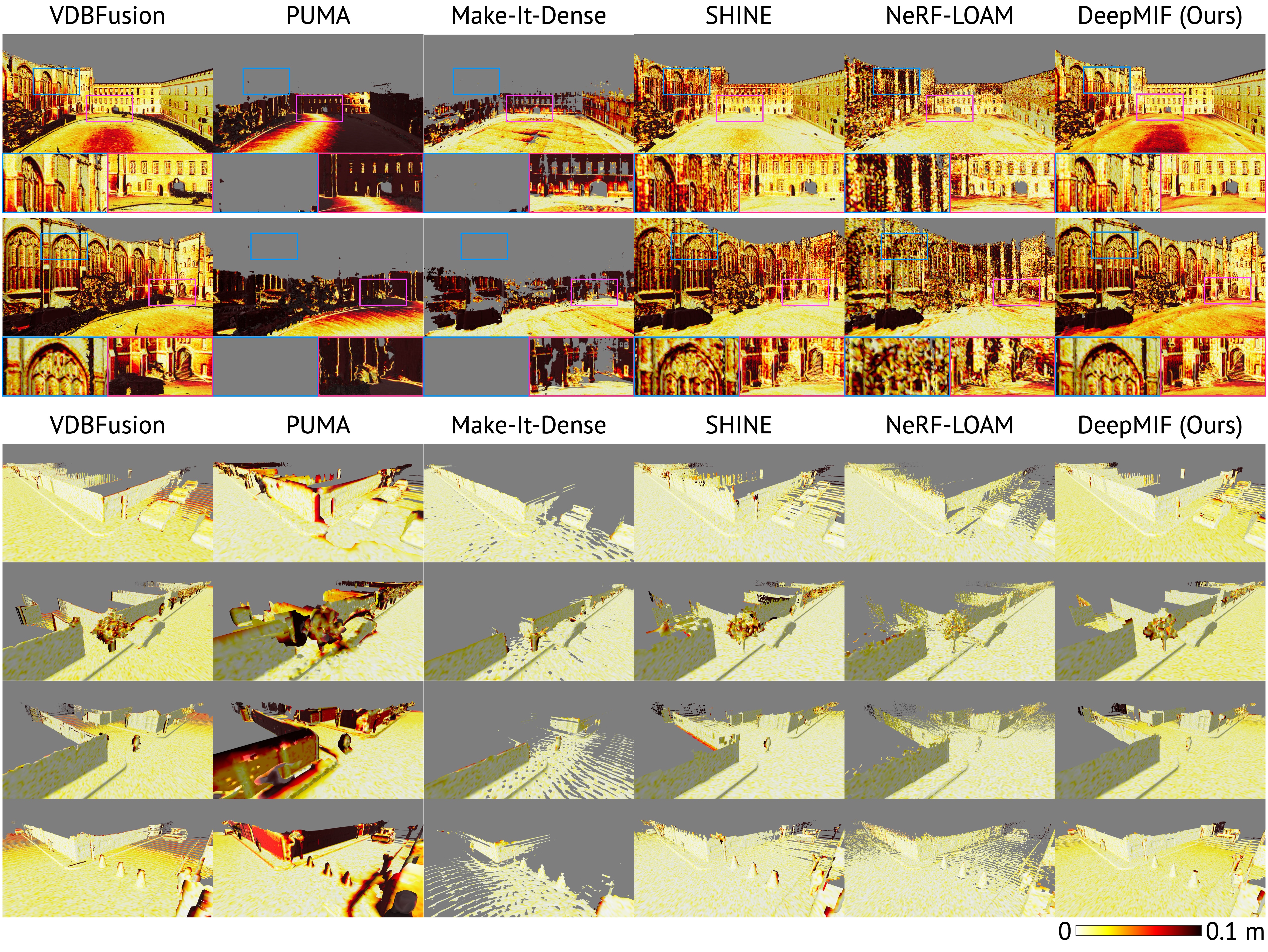
Figure 4: Qualitative large-scale 3D mapping results on Newer College [48] (upper part) and Mai City [13] (lower part). For Newer College, our algorithm delivers significantly cleaner reconstruction compared to NeRF-LOAM [10], more complete results compared to PUMA [13] and Make-It-Dense [14], and performs qualitatively comparably to VDBFusion [12] and SHINE [6]. Similarly for Mai City, our algorithm obtains more complete, robust reconstructions, particularly at object edges.

IV-A Experimental Setup

Baselines

We use a variety of state-of-the-art methods designed for large-scale, outdoor LiDAR 3D mapping, as baselines. SHINE [6] is a neural surface fitting method integrating a hierarchical latent grid. NeRF-LOAM [10] is a NeRF-based LiDAR 3D mapping method. Make-It-Dense [14] is a learnable, self-supervised 3D scan completion method. PUMA [13] is a surface reconstruction method based on PSR [33]. VDBFusion [12] is a depth fusion method adapted to sparse LiDAR 3D scans.

Benchmark Datasets

We use three open-source datasets to evaluate our method. Mai City [13] is a simulated benchmark for assessing 3D mapping performance, including a single large-scale CAD scene and synthetic measurements obtained by a virtual 64-beam LiDAR scanning. Newer College [48] is a real-world dataset captured by a hand-held 64-beam LiDAR sensor and including a high-quality reference point cloud obtained by an industrial 3D laser scanner. We additionally include qualitative results obtained on KITTI autonomous driving dataset including a 64-beam LiDAR scanner [51].

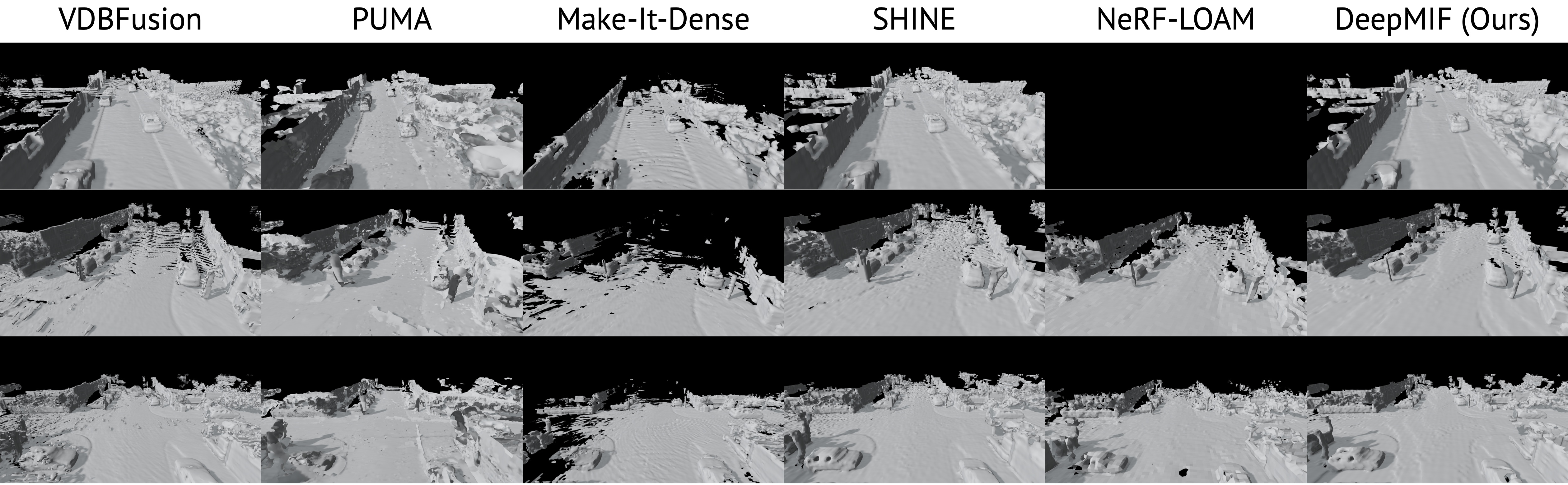
Figure 5: Qualitative large-scale 3D mapping results on KITTI [51]. Compared to baselines, our method produces more complete, smooth, and sharp reconstruction.

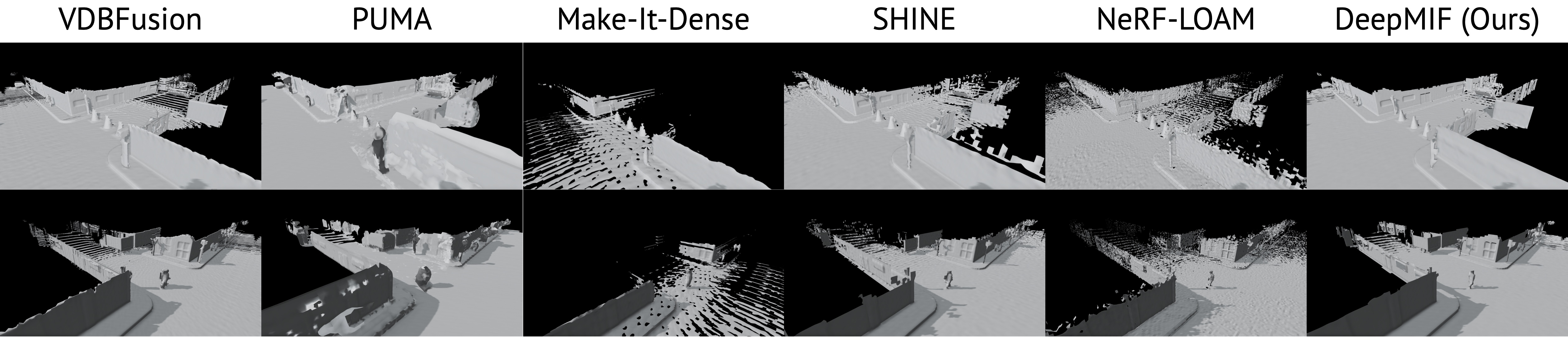
Figure 6: Qualitative large-scale 3D mapping results on MaiCity [13]. Compared to baselines, our method produces more complete, smooth, and sharp reconstruction.

Evaluation Metrics

Following standard practices [13, 6], we report performance measures commonly used for evaluating 3D surface reconstruction. We uniformly sample both the predicted and the ground-truth meshes at a resolution of 2 cm to generate a point cloud. Accuracy (Acc.) corresponds to an average distance between the sampled points and the ground-truth mesh. Completion (Compl.), measures average distances from points sampled on the ground-truth mesh to the predicted mesh, truncated when exceeding 2 m. Chamfer distance (Chamfer L2) is the squared mean of accuracy and completion. Precision (Prec.) and Recall (Rec.) represent the ratio of points within a max distance threshold (we use 10 cm) from the predicted to the ground-truth mesh and vice versa, respectively. Finally, we report the F-Score, a harmonic mean of Precision and Recall. We additionally opted to assess the perceptual quality of produced 3D maps in comparison to reference meshes, as similarly utilized in [52]. For this, we produce shaded renders from multiple viewing directions under a constant illumination, compute perceptual $\text{RMSE}_{\text{v}}$ [52] and LPIPS [53] measures, and report their averages.

Training Details

We use the AdamW optimizer with a learning rate of 0.01, $\epsilon=10^{-15}$, weight decay of $10^{-7}$, and perform learning rate decay steps at 10K and 50K iterations. Training employs batches of ray samples, where each input comprises multiple consecutive points along a LiDAR scan ray. This results in a total of $N\times B$ points processed per iteration, where $N$ is the number of samples and $B$ is the batch size. We give the sampling details in Sec. III-D. We train for 10K–20K iterations, taking approximately 30-60 min on an NVIDIA RTX A5000 GPU and Intel(R) Core(TM) i7-13700 CPU.

IV-B Comparisons to State-of-the-Art

Results on Real-World Newer College Dataset and Synthetic Mai City Dataset

In Tab. I, we report a quantitative comparison of our method against baseline approaches. All methods were evaluated with a reconstruction resolution of 10 cm. While Make-It-Dense [14] achieves the best values of accuracy measure, its reconstructions are highly incomplete and distorted as observed in Fig. 4, leading to poor completion performance. Our method demonstrates performance comparable to VDBFusion and SHINE-Mapping in both accuracy and completion, even surpassing other methods or achieving second place in terms of Completion % and F-Score. However, due to limitations of the accuracy metric (focusing solely on predicted meshes) and potential saturation by bloated predictions in the completion metric, point cloud comparisons may not fully capture mesh smoothness or completion. Therefore, a complementary perceptual evaluation is presented in Tab. III.

In Tab. III, we show quantitative evaluation of the perceptual performance of reconstruction methods on the Newer College and Mai City datasets. The evaluation employs $\text{RMSE}_{\text{v}}$ and LPIPS metrics. For the Mai City dataset, we uniformly sample 20 poses along the road, each encompassing 8 views along a $360^{\circ}$ circumference, resulting in a total of 160 views. In the Newer College dataset, 64 poses were uniformly sampled along the ground truth trajectory and progressively elevated by 2 meters at each step for a total of 5 elevations, yielding 320 views. Subsequently, the rendered views were compared with the ground truth mesh obtained by applying Poisson reconstruction to the ground truth point cloud. The results demonstrate that our method outperforms other methods on both datasets according to both metrics, which indicates a visually closer resemblance between our reconstructions and the ground truth meshes. Examples of rendered views can be seen in Fig. 6, qualitatively demonstrating superiority of our method in completion and reconstruction performance compared to baseline methods.

Qualitative Results on KITTI

In Fig. 5, we present a qualitative comparison of reconstruction methods on the KITTI dataset. VDBFusion demonstrates strong object reconstruction but suffers from missing areas and artifacts. SHINE-Mapping achieves good reconstruction quality but exhibits noisy, uneven, and incomplete surfaces. NeRF-LOAM generates similar surfaces to SHINE-Mapping but struggles with incomplete reconstructions more. Make-It-Dense exhibits good reconstruction quality but lacks scene completion, while PUMA prioritizes completion at the expense of reconstruction quality and suffers artifacts. Our method outperforms others in completion of missing parts and achieves smoother surfaces overall.

IV-C Ablative Studies

Contributions of Individual Loss Terms

In Tab. IV, we detail an ablation study on the Mai City dataset to show the influence of each loss term on reconstruction quality. Excluding the surface loss entirely leads to reconstruction failure. While the combined sign and monotonicity loss inherently incorporates this information, we suspect training instability. Omitting either monotonicity or sign loss yields comparable meshes. Notably, sign loss improves completion, while monotonicity loss enhances accuracy. Utilizing all loss terms together outperforms all other configurations on every metric except the completion % which is similar to best performing case. The eikonal loss, while highly effective for reconstruction quality, was excluded to prevent impacting the ablation study’s focus.

Losses			Metrics
Surface	Sign	Mono.	$\acc\downarrow$	$\comp\downarrow$	$\cd\downarrow$	$\pre\uparrow$	$\rec\uparrow$	$\fscore\uparrow$
	✓	✓	Fails
✓	✓		0.052	0.064	0.127	89.051	93.689	91.311
✓		✓	0.046	0.103	0.217	89.553	87.048	88.282
✓	✓	✓	0.044	0.057	0.122	90.121	93.244	91.656

TABLE IV: An ablation study on Mai City to evaluate the contribution of individual loss terms where each term was isolated. We report the corresponding accuracy, completion, Chamfer-L2 (Ch. L2) distance, accuracy % within 10cm, and F-Score for each configuration. The best performing combination is denoted in bold. The results demonstrate that using all loss terms together outperforms all other combinations.

V Conclusion

We proposed an implicit representation suitable for LiDAR-based 3D scene modelling. Compared to existing representations such as signed distance functions, our monotonic implicit function does not require exact, dense point samples to be trained from sparse point sets acquired by modern scanners such as LiDARs. Our implicit field can be easily integrated in a large-scale 3D mapping system by enforcing a monotonicity loss along sensosr scanning rays. We have demonstrated the capabilities of our method with a synthetic Mai City and a real-world Newer College and KITTI benchmarks, where attained strong performance compared to five baseline approaches.

References

- [1] J. J. Park, P. Florence, J. Straub, R. Newcombe, and S. Lovegrove, “Deepsdf: Learning continuous signed distance functions for shape representation,” in Proceedings of the IEEE/CVF conference on computer vision and pattern recognition, 2019, pp. 165–174.
- [2] L. Mescheder, M. Oechsle, M. Niemeyer, S. Nowozin, and A. Geiger, “Occupancy networks: Learning 3d reconstruction in function space,” in Proceedings of the IEEE/CVF conference on computer vision and pattern recognition, 2019, pp. 4460–4470.
- [3] P. Wang, L. Liu, Y. Liu, C. Theobalt, T. Komura, and W. Wang, “Neus: Learning neural implicit surfaces by volume rendering for multi-view reconstruction,” Advances in Neural Information Processing Systems, vol. 34, pp. 27 171–27 183, 2021.
- [4] J. Wang, T. Bleja, and L. Agapito, “Go-surf: Neural feature grid optimization for fast, high-fidelity rgb-d surface reconstruction,” in 2022 International Conference on 3D Vision (3DV). IEEE, 2022, pp. 433–442.
- [5] D. Azinović, R. Martin-Brualla, D. B. Goldman, M. Nießner, and J. Thies, “Neural rgb-d surface reconstruction,” in Proceedings of the IEEE/CVF Conference on Computer Vision and Pattern Recognition, 2022, pp. 6290–6301.
- [6] X. Zhong, Y. Pan, J. Behley, and C. Stachniss, “Shine-mapping: Large-scale 3d mapping using sparse hierarchical implicit neural representations,” in 2023 IEEE International Conference on Robotics and Automation (ICRA). IEEE, 2023, pp. 8371–8377.
- [7] C. Shi, F. Tang, Y. Wu, X. Jin, and G. Ma, “Accurate implicit neural mapping with more compact representation in large-scale scenes using ranging data,” IEEE Robotics and Automation Letters, 2023.
- [8] S. Song, J. Zhao, K. Huang, J. Lin, C. Ye, and T. Feng, “N3-mapping: Normal guided neural non-projective signed distance fields for large-scale 3d mapping,” arXiv preprint arXiv:2401.03412, 2024.
- [9] S. Isaacson, P.-C. Kung, M. Ramanagopal, R. Vasudevan, and K. A. Skinner, “Loner: Lidar only neural representations for real-time slam,” IEEE Robotics and Automation Letters, 2023.
- [10] J. Deng, Q. Wu, X. Chen, S. Xia, Z. Sun, G. Liu, W. Yu, and L. Pei, “Nerf-loam: Neural implicit representation for large-scale incremental lidar odometry and mapping,” in Proceedings of the IEEE/CVF International Conference on Computer Vision, 2023, pp. 8218–8227.
- [11] L. Wiesmann, T. Guadagnino, I. Vizzo, N. Zimmerman, Y. Pan, H. Kuang, J. Behley, and C. Stachniss, “Locndf: Neural distance field mapping for robot localization,” IEEE Robotics and Automation Letters, 2023.
- [12] I. Vizzo, T. Guadagnino, J. Behley, and C. Stachniss, “Vdbfusion: Flexible and efficient tsdf integration of range sensor data,” Sensors, vol. 22, no. 3, p. 1296, 2022.
- [13] I. Vizzo, X. Chen, N. Chebrolu, J. Behley, and C. Stachniss, “Poisson surface reconstruction for lidar odometry and mapping,” in 2021 IEEE International Conference on Robotics and Automation (ICRA). IEEE, 2021, pp. 5624–5630.
- [14] I. Vizzo, B. Mersch, R. Marcuzzi, L. Wiesmann, J. Behley, and C. Stachniss, “Make it dense: Self-supervised geometric scan completion of sparse 3d lidar scans in large outdoor environments,” IEEE Robotics and Automation Letters, vol. 7, no. 3, pp. 8534–8541, 2022.
- [15] M. Berger, A. Tagliasacchi, L. M. Seversky, P. Alliez, G. Guennebaud, J. A. Levine, A. Sharf, and C. T. Silva, “A survey of surface reconstruction from point clouds,” in Computer graphics forum, vol. 36, no. 1. Wiley Online Library, 2017, pp. 301–329.
- [16] M. Zollhöfer, P. Stotko, A. Görlitz, C. Theobalt, M. Nießner, R. Klein, and A. Kolb, “State of the art on 3d reconstruction with rgb-d cameras,” in Computer graphics forum, vol. 37, no. 2. Wiley Online Library, 2018, pp. 625–652.
- [17] Y. Xie, T. Takikawa, S. Saito, O. Litany, S. Yan, N. Khan, F. Tombari, J. Tompkin, V. Sitzmann, and S. Sridhar, “Neural fields in visual computing and beyond,” in Computer Graphics Forum, vol. 41, no. 2. Wiley Online Library, 2022, pp. 641–676.
- [18] H. Pfister, M. Zwicker, J. Van Baar, and M. Gross, “Surfels: Surface elements as rendering primitives,” in Proceedings of the 27th annual conference on Computer graphics and interactive techniques, 2000, pp. 335–342.
- [19] B. Curless and M. Levoy, “A volumetric method for building complex models from range images,” in Proceedings of the 23rd annual conference on Computer graphics and interactive techniques, 1996, pp. 303–312.
- [20] R. A. Newcombe, S. Izadi, O. Hilliges, D. Molyneaux, D. Kim, A. J. Davison, P. Kohi, J. Shotton, S. Hodges, and A. Fitzgibbon, “Kinectfusion: Real-time dense surface mapping and tracking,” in 2011 10th IEEE international symposium on mixed and augmented reality. Ieee, 2011, pp. 127–136.
- [21] S. Ilic and P. Fua, “Implicit meshes for surface reconstruction,” IEEE Transactions on Pattern Analysis and Machine Intelligence, vol. 28, no. 2, pp. 328–333, 2005.
- [22] M. Nießner, M. Zollhöfer, S. Izadi, and M. Stamminger, “Real-time 3d reconstruction at scale using voxel hashing,” ACM Transactions on Graphics (ToG), vol. 32, no. 6, pp. 1–11, 2013.
- [23] A. Hornung, K. M. Wurm, M. Bennewitz, C. Stachniss, and W. Burgard, “Octomap: An efficient probabilistic 3d mapping framework based on octrees,” Autonomous robots, vol. 34, pp. 189–206, 2013.
- [24] F. Steinbrücker, J. Sturm, and D. Cremers, “Volumetric 3d mapping in real-time on a cpu,” in 2014 IEEE international conference on robotics and automation (ICRA). IEEE, 2014, pp. 2021–2028.
- [25] G. Riegler, A. O. Ulusoy, H. Bischof, and A. Geiger, “Octnetfusion: Learning depth fusion from data,” in 2017 International Conference on 3D Vision (3DV). IEEE, 2017, pp. 57–66.
- [26] A. Dai, C. Diller, and M. Nießner, “Sg-nn: Sparse generative neural networks for self-supervised scene completion of rgb-d scans,” in Proceedings of the IEEE/CVF Conference on Computer Vision and Pattern Recognition, 2020, pp. 849–858.
- [27] X. Yan, J. Gao, J. Li, R. Zhang, Z. Li, R. Huang, and S. Cui, “Sparse single sweep lidar point cloud segmentation via learning contextual shape priors from scene completion,” in Proceedings of the AAAI Conference on Artificial Intelligence, vol. 35, no. 4, 2021, pp. 3101–3109.
- [28] R. Cheng, C. Agia, Y. Ren, X. Li, and L. Bingbing, “S3cnet: A sparse semantic scene completion network for lidar point clouds,” in Conference on Robot Learning. PMLR, 2021, pp. 2148–2161.
- [29] Y. Li, Z. Yu, C. Choy, C. Xiao, J. M. Alvarez, S. Fidler, C. Feng, and A. Anandkumar, “Voxformer: Sparse voxel transformer for camera-based 3d semantic scene completion,” in Proceedings of the IEEE/CVF Conference on Computer Vision and Pattern Recognition, 2023, pp. 9087–9098.
- [30] L. Roldao, R. de Charette, and A. Verroust-Blondet, “Lmscnet: Lightweight multiscale 3d semantic completion,” in 2020 International Conference on 3D Vision (3DV). IEEE, 2020, pp. 111–119.
- [31] Z. Xia, Y. Liu, X. Li, X. Zhu, Y. Ma, Y. Li, Y. Hou, and Y. Qiao, “Scpnet: Semantic scene completion on point cloud,” in Proceedings of the IEEE/CVF Conference on Computer Vision and Pattern Recognition, 2023, pp. 17 642–17 651.
- [32] M. Kazhdan, M. Bolitho, and H. Hoppe, “Poisson surface reconstruction,” in Proceedings of the fourth Eurographics symposium on Geometry processing, vol. 7, 2006, p. 0.
- [33] M. Kazhdan and H. Hoppe, “Screened poisson surface reconstruction,” ACM Transactions on Graphics (ToG), vol. 32, no. 3, pp. 1–13, 2013.
- [34] M. Atzmon and Y. Lipman, “Sal: Sign agnostic learning of shapes from raw data,” in Proceedings of the IEEE/CVF Conference on Computer Vision and Pattern Recognition, 2020, pp. 2565–2574.
- [35] P. Mullen, F. De Goes, M. Desbrun, D. Cohen-Steiner, and P. Alliez, “Signing the unsigned: Robust surface reconstruction from raw pointsets,” in Computer Graphics Forum, vol. 29, no. 5. Wiley Online Library, 2010, pp. 1733–1741.
- [36] J. Chibane, G. Pons-Moll, et al., “Neural unsigned distance fields for implicit function learning,” Advances in Neural Information Processing Systems, vol. 33, pp. 21 638–21 652, 2020.
- [37] J. Zhou, B. Ma, S. Li, Y.-S. Liu, and Z. Han, “Learning a more continuous zero level set in unsigned distance fields through level set projection,” in Proceedings of the IEEE/CVF international conference on computer vision, 2023, pp. 3181–3192.
- [38] J. Ye, Y. Chen, N. Wang, and X. Wang, “Gifs: Neural implicit function for general shape representation,” in Proceedings of the IEEE/CVF Conference on Computer Vision and Pattern Recognition, 2022, pp. 12 829–12 839.
- [39] C. Jiang, A. Sud, A. Makadia, J. Huang, M. Nießner, T. Funkhouser, et al., “Local implicit grid representations for 3d scenes,” in Proceedings of the IEEE/CVF Conference on Computer Vision and Pattern Recognition, 2020, pp. 6001–6010.
- [40] R. Chabra, J. E. Lenssen, E. Ilg, T. Schmidt, J. Straub, S. Lovegrove, and R. Newcombe, “Deep local shapes: Learning local sdf priors for detailed 3d reconstruction,” in Computer Vision–ECCV 2020: 16th European Conference, Glasgow, UK, August 23–28, 2020, Proceedings, Part XXIX 16. Springer, 2020, pp. 608–625.
- [41] S. Peng, M. Niemeyer, L. Mescheder, M. Pollefeys, and A. Geiger, “Convolutional occupancy networks,” in Computer Vision–ECCV 2020: 16th European Conference, Glasgow, UK, August 23–28, 2020, Proceedings, Part III 16. Springer, 2020, pp. 523–540.
- [42] T. Takikawa, J. Litalien, K. Yin, K. Kreis, C. Loop, D. Nowrouzezahrai, A. Jacobson, M. McGuire, and S. Fidler, “Neural geometric level of detail: Real-time rendering with implicit 3d shapes,” in Proceedings of the IEEE/CVF Conference on Computer Vision and Pattern Recognition, 2021, pp. 11 358–11 367.
- [43] Z. Yu, S. Peng, M. Niemeyer, T. Sattler, and A. Geiger, “Monosdf: Exploring monocular geometric cues for neural implicit surface reconstruction,” Advances in neural information processing systems, vol. 35, pp. 25 018–25 032, 2022.
- [44] Z. Zhu, S. Peng, V. Larsson, W. Xu, H. Bao, Z. Cui, M. R. Oswald, and M. Pollefeys, “Nice-slam: Neural implicit scalable encoding for slam,” in Proceedings of the IEEE/CVF Conference on Computer Vision and Pattern Recognition, 2022, pp. 12 786–12 796.
- [45] B. Mildenhall, P. P. Srinivasan, M. Tancik, J. T. Barron, R. Ramamoorthi, and R. Ng, “Nerf: Representing scenes as neural radiance fields for view synthesis,” Communications of the ACM, vol. 65, no. 1, pp. 99–106, 2021.
- [46] S. Koch, A. Matveev, Z. Jiang, F. Williams, A. Artemov, E. Burnaev, M. Alexa, D. Zorin, and D. Panozzo, “Abc: A big cad model dataset for geometric deep learning,” in Proceedings of the IEEE/CVF conference on computer vision and pattern recognition, 2019, pp. 9601–9611.
- [47] T. Lewiner, H. Lopes, A. W. Vieira, and G. Tavares, “Efficient implementation of marching cubes’ cases with topological guarantees,” Journal of graphics tools, vol. 8, no. 2, pp. 1–15, 2003.
- [48] M. Ramezani, Y. Wang, M. Camurri, D. Wisth, M. Mattamala, and M. Fallon, “The newer college dataset: Handheld lidar, inertial and vision with ground truth,” in 2020 IEEE/RSJ International Conference on Intelligent Robots and Systems (IROS). IEEE, 2020, pp. 4353–4360.
- [49] A. Gropp, L. Yariv, N. Haim, M. Atzmon, and Y. Lipman, “Implicit geometric regularization for learning shapes,” in International Conference on Machine Learning. PMLR, 2020, pp. 3789–3799.
- [50] T. Salimans and D. P. Kingma, “Weight normalization: A simple reparameterization to accelerate training of deep neural networks,” 2016.
- [51] A. Geiger, P. Lenz, and R. Urtasun, “Are we ready for autonomous driving? the kitti vision benchmark suite,” in 2012 IEEE conference on computer vision and pattern recognition. IEEE, 2012, pp. 3354–3361.
- [52] O. Voynov, A. Artemov, V. Egiazarian, A. Notchenko, G. Bobrovskikh, E. Burnaev, and D. Zorin, “Perceptual deep depth super-resolution,” in Proceedings of the IEEE/CVF International Conference on Computer Vision, 2019, pp. 5653–5663.
- [53] R. Zhang, P. Isola, A. A. Efros, E. Shechtman, and O. Wang, “The unreasonable effectiveness of deep features as a perceptual metric,” in Proceedings of the IEEE conference on computer vision and pattern recognition, 2018, pp. 586–595.