A Brief Survey of Fluctuation-induced Interactions in Micro- and Nano-systems and One Exactly Solvable Model as Example

Abstract

Fluctuations exist in any material object $A$. If $A$ has non-zero temperature $T$, one speaks about thermal fluctuations. If $A$ is at very low $T$, the fluctuations are of quantum origin. Interesting effects appear if two bodies $A$ and $B$ are separated by a fluctuating medium $C$ (say a vacuum, or a fluid close to its critical point) when the fluctuations are long-ranged, i.e., they decay according to a power-law with the distance. Then the changes of fluctuations in $C$ due to the surfaces and constituents of $A$ are also felt by $B$, and vice versa, which leads to a fluctuation induced force (FIF) between them. This force persists in addition to the direct influence of $A$ on $B$ (say, via gravity or Coulomb’s force). These FIF’s can be of attractive or repulsive character. They may play crucially important role on phenomena involving objects with length scale comparative with the Universe, as well as to the tiny objects relevant for MEMS and NEMS. In the current article we present some basic facts for the FIF and their diversity. Then on the example of one dimensional Ising model with a defect bond we present some new analytical results for such forces.

1 Introduction in Fluctuation-induce Forces: A Brief Review

We consider two macroscopic or mesoscopic material bodies $A$ and $B$, separated by a fluctuating medium $C$. We always suppose that the degrees of freedom can enter and leave the region between the interacting objects. There are, however, two important subcases - one in which the $C$ is in some contact with a reservoir, i.e., its constituents can enter and leave the part of the space occupied by $A$ and $B$. In this case on speaks about the Casimir force. In the second case, the system is itself bounded, so that some quantity characterizing the amount of material in $C$ is conserved. Then, on speaks about the recently introduced, see the Letter DR2022 , and still not well studied, Helmholtz force. Both these forces are examples of the fluctuation induced forces and they do exist because the medium $C$ fluctuates and, when the force decays algebraically with the distance so do the correlations of the fluctuations in $C$. Many other examples of such forces are presented in Ref. DD2022 .

Maybe the first study of a fluctuation induced force is due to A. Einstein E07 . Having in mind a standard capacitor at nonzero temperature $T$, as early as in 1907 he studied the voltage fluctuations between its plates and even concluded that the corresponding effect can be measured.

Presently, the most famous example of a fluctuation-induced interaction is the quantum electrodynamic (QED) Casimir effect C48 ; MT97 ; KG99 ; M2001 ; BKMM2009 . Nowadays, investigations devoted to that effect are performed on many fronts of research ranging from attempts to unify the four fundamental forces of nature MT97 ; M2001 ; M2004 to rather practical issues such as the design and the performance of MEMS and NEMS GLR2008 ; KMM2011 ; RCJ2011 ; FAKA2014 ; FMRA2014 .

In the QED Casimir effect the medium $C$ is the vacuum; the presence of two conducting plates (the interacting objects $A$ and $B$) modifies the zero point energy of the electromagnetic field and leads to an attractive force (normalized per area, i.e. to the so-called Casimir pressure)

$$F_{\rm Cas}^{(\rm QED)}(L)=-\frac{\pi^{2}}{240}\frac{\hbar c}{L^{4}}=-1.3\times 10^{-3}\frac{1}{(L/{\rm\mu m})^{4}}{\rm\frac{N}{m^{2}}},$$ (1)

where $L$ is the separation between the plates, $\hbar$ and $c$ are the Planck constant ($\hbar=h/(2\pi)$), and the speed of light in vacuum, respectively. The QED Casimir effect is one of the rare manifestations of quantum physics at the macroscopic scale, like super-conductivity and super-fluidity.

At non-zero temperature, as it shall be expected, the thermal fluctuations come into play, giving rise to additional temperature-dependent interactions. When applied to realistic materials, the material properties of the bodies $A,B$ and the medium $C$ get also involved via their general dielectric and conductive properties. This has been done by E. M. Lifshitz et al.L56 ; L.E.Dzyaloshinskii1961 , see also MN76 ; P2006 . There the material properties enter via the frequency-dependent dielectric permittivities $\varepsilon^{(A)}(\omega)$, $\varepsilon^{(B)}(\omega)$, and $\varepsilon^{(C)}(\omega)$. In the limit of small separations (but still large compared with molecular scales) the Casimir force approaches the more familiar van der Waals force DLP61r ; BKMM2009 . From Lifshitz theory one can infer DLP61r that there is a possibility to observe QED Casimir repulsion in the film geometry if the two half-spaces (A) and (B) forming the plates and confining the film (C) exhibit permittivities which fulfill the relationship

$$\varepsilon^{(B)}(i\xi)<\varepsilon^{(C)}(i\xi)<\varepsilon^{(A)}(i\xi).$$ (2)

Experimentally repulsion occurs if the inequality in Eq. (2) holds over a sufficiently wide frequency range. Actually this is a widespread phenomenon shared by all substrate-fluid systems which show complete wetting Di88 . Accordingly Casimir repulsion is a common feature and has been already observed - see, e.g., Ref. MCP2009 .

Thirty years after H. B. G. Casimir, in 1978 M. Fisher and P-G. de Gennes FG78 have shown that a very similar fluctuation-induced effect exists in fluids. This is now the widely-investigated critical Casimir effect (CCE). It results from the fluctuations of an order parameter and, more generally, from the thermodynamics of the medium supporting that order parameter in the vicinity of a critical point. Recently, a review on the exact results available for the CCE has been published in Ref. DD2022 . On different aspects of this effect overviews can be found in Krech1994 ; BDT2000 ; MD2018 ; DD2022 ; Gambassi2023 . For the critical Casimir effect (CCE) the expression, analogous to Eq. (1), exist at the critical point $T=T_{c}$ of the fluid $C$. For the $(d=3)$-dimensional system one can write the critical Casimir force (CCF) per unit area, i.e., the Casimir pressure, in the form

$$F_{{\rm Cas}}^{(\tau)}(T=T_{c},L)\simeq 8.1\times 10^{-3}\dfrac{\Delta^{(\tau)}(d=3)}{(L/\mu{\rm m})^{3}}\dfrac{T_{c}}{T_{\rm roon}}\dfrac{{\rm N}}{{\rm m^{2}}},$$ (3)

where $T_{\rm room}=20$ ^∘C (293.15 K). Here $\Delta^{(\tau)}$ is the so-called Casimir amplitude that depends on the bulk and surface universality classes (see below) of the system and the applied boundary conditions $\tau$. For most systems and boundary conditions one has $\Delta^{(\tau)}(d)={\cal O}(1)$.

Thus, the both forces, the quantum and the critical one, can be of the same order of magnitude, i.e., they both can be essential, measurable and obviously significant at or below the micrometer length scale. Let us stress that $\Delta^{(\tau)}(d)$ can be both positive and negative, i.e., $F_{{\rm Cas}}^{(\tau)}(T,L)$ can be both attractive and repulsive. The accepted terminology terms the negative force as attractive one.

In recent Letter DR2022 we have introduced and studied a Helmholtz fluctuation induced force. It is a force in which an integral quantity value of the order parameter characterizing the system is fixed (say the total magnetization in the system). We stress, that in standard envisaged applications of, say, the equilibrium Ising model to binary alloys or binary liquids, the case with order parameter fixed must be addressed, provided that one considers finite systems and insists on a rigorous analytical treatment. In Refs. DR2022 ; Dantchev2023b via deriving there exact results on the example of Ising chain with fixed magnetization under periodic and antiperiodic boundary conditions, we have established a very different behavior of the Helmholtz force from that one of the Casimir force, in the same model and under the same boundary conditions. It is interesting to note that, actually, under periodic boundary conditions the studied Helmholtz force has a behavior similar to the one appearing in some versions of the big bang theory — strong repulsion at high temperatures, transitioning to moderate attraction for intermediate values of the temperature, and then back to repulsion, albeit much weaker than during the initial period of highest temperature.

In order to be concrete and avoid any misunderstandings, let us remind the definitions of the critical Casimir and Helmholtz forces — the Casimir force in the grand canonical ensemble (GCE), and its analogue in the canonical ensemble (CE) — the Helmholtz force .

In the general case, we envisage a $d$-dimensional system with a film geometry $\infty^{d-1}\times L$, $L\equiv L_{\perp}$, and with boundary conditions $\zeta$ imposed along the spatial direction of finite extent $L$. Let us take ${\cal F}_{{\rm tot}}^{(\zeta)}(L,T,h)$ to be the total (Gibbs) free energy of such a system within the GCE, where $T$ is the temperature and $h$ is the magnetic field. Then, if $f^{(\zeta)}(T,h,L)\equiv\lim_{A\to\infty}{\cal F}_{{\rm tot}}^{(\zeta)}/A$ is the free energy per area $A$ of the system, one can define the Casimir force for critical systems in the grand-canonical $(T-h)$-ensemble, see, e.g. Ref. Krech1994 ; BDT2000 ; MD2018 ; DD2022 ; Gambassi2023 , as:

$$\beta F_{\rm Cas}^{(\zeta)}(L,T,h)\equiv-\frac{\partial}{\partial L}f_{\rm ex}^{(\zeta)}(L,T,h)$$ (4)

where

$$f_{\rm ex}^{(\zeta)}(L,T,h)\equiv f^{(\zeta)}(L,T,h)-Lf_{b}(T,h)$$ (5)

is the so-called excess (over the bulk) free energy per area and per $\beta^{-1}=k_{B}T$.

Along these lines, if $M$ is the fixed value of the total magnetization, the definition of the Helmholtz fluctuation induced force DR2022 ; Dantchev2023b in the canonical $(T-M)$-ensemble is:

$$\beta F_{\rm H}^{(\zeta)}(L,T,M)\equiv-\frac{\partial}{\partial L}f_{\rm ex}^{(\zeta)}(L,T,M)$$ (6)

and

$$f_{\rm ex}^{(\zeta)}(L,T,M)\equiv f^{(\zeta)}(L,T,M)-Lf_{H}(T,m).$$ (7)

In the above formula, $m=\lim_{L,A\to\infty}M/(LA)$ is the average magnetization, and $f_{H}(T,m)$ is the Helmholtz free energy density of the “infinite” system. In the remainder of this article we will take $L=Na$, where $N$ is an integer number, and without loss of generality we set the lattice spacing $a=1$.

We stress that the definition and existence of Helmholtz force is by no means limited to the Ising chain and can be addressed, in principle, in any model of interest.

We note that a somewhat elaborate information about the ensemble behaviour of fluctuation-induced forces has not yet been obtained.

In the remainder of the current text, on the example of the well known one-dimensional Ising model, we present some new both exact analytical and numerical results for the behavior of the Casimir and Helmholtz forces. We will consider the case of the Ising model with a defect bond. The definition of the model is given in Sec. 2. The derivation of the partition function of the model in GCE is presented in Sec. 3. General results for the behavior of the free energy density of the finite chain with defect bond and how from the results presented there one easily can obtain those for periodic, antiperiodic and Dirichlet boundary conditions are given in Sec. 3.1. The behavior of the Casimir force in Ising chain with defect bond is discussed in Sec. 4. The derivation of the partition function in canonical ensemble is presented in Sec. 5. The behavior of the Helmholtz is then discussed and visualized in Sec. 6. The article closes with a discussion and concluding remarks section 7.

2 The Model

Let us consider a one-dimensional Ising chain of $N$ spins $(S_{i}\pm 1,i=1,..,N)$. We suppose that the interaction between them $J$ is of a ferromagnetic type, i.e., that $J>0$. The Hamiltonian of the model is given by

$${\cal H}^{(\zeta)}=-J\sum_{i=1}^{N-1}S_{i}S_{i+1}-J_{BC}S_{1}S_{N}+h\sum_{i=1}^{N}S_{i}.$$ (8)

This form of the Hamiltonian allows for the discussion of different boundary conditions: when $J_{BC}=-J,J,0,J_{a}$ one has periodic (PBC’s), antiperiodic (ABC’s), or Dirichlet-Dirichlet (DBC’s) (also termed free, or missing neighbors), boundary conditions, respectively. Here we focus on the more general case when $J_{BC}=J_{a}$, where $J_{a}$ can have both positive or negative values, which we will call a model with a defect bond. In the last case we will use the notation $\zeta={\rm db}$.

The main quantity of interest in the statistical mechanics is the partition function. For the considered model the partition function is given by

$$Z_{\rm GC}^{\rm(db)}(N,K,K_{a},h)=\sum_{\{S_{i}\}}\exp\left[-\beta{\cal H}^{{\rm(db)}}\right].$$ (9)

Here $K=\beta J$ and $K_{a}=\beta J_{a}$, while ${\rm(db)}$ depicts the considered boundary conditions.

3 On the Behavior of the Model in Grand Canonical Ensemble

The partition function of the system can be written in the form

$$Z_{\rm GC}^{\rm(db)}(N,K,K_{a},h) = \sum_{\{S_{i}=\pm 1\}}\exp\left[K\left(S_{1}S_{2}+S_{2}S_{3}+\cdots+S_{N-2}S_{N-1}\right)+K_{a}S_{1}S_{N}\right.$$ (10)

$$\left.+h\left(S_{1}+S_{2}+\cdots+S_{N-1}+S_{N}\right)\right].$$

It is helpful to cast the above formula as follows

$$Z_{\rm GC}^{\rm db}(N,K,K_{a},h)=$$ (11)

$$\sum_{\{S_{i}\}}\exp\left[\frac{1}{2}\left(hS_{1}+hS_{2}\right)+KS_{1}S_{2}\right]\exp\left[\frac{1}{2}\left(hS_{2}+hS_{3}\right)+KS_{2}S_{3}\right]$$

$$\times\cdots\times\exp\left[\frac{1}{2}\left(hS_{N-1}+hS_{N}\right)+KS_{N-1}S_{N}\right]\exp\left[\frac{1}{2}\left(hS_{N}+hS_{1}\right)+K_{a}S_{N}S_{1}\right].$$

Introducing the matrices

$${\mathbf{T}}=\begin{pmatrix}\exp\left(K+h\right)&\exp\left(-K\right)\\ \\ \exp\left(-K\right)&\exp\left(K-h\right)\end{pmatrix},\quad\mbox{and}\quad{\mathbf{T}}_{a}=\begin{pmatrix}\exp\left(K_{a}+h\right)&\exp\left(-K_{a}\right)\\ \\ \exp\left(-K_{a}\right)&\exp\left(K_{a}-h\right)\end{pmatrix},$$ (12)

it is easy to show that

$$Z_{\rm GC}^{\rm(db)}(N,K,K_{a},h)={\rm Tr}\,\left[{\mathbf{T}}^{N-1}{\mathbf{T}}_{a}\right].$$ (13)

The matrix ${\mathbf{T}}$ is usually called transfer matrix. In the remainder we will need its eigenvalues. They are, customarily, denoted by $\lambda_{1}$ and $\lambda_{2}$ and read

$$\lambda_{1,2}(K,h)=e^{K}\left(\cosh h\pm\sqrt{e^{-4K}+\sinh^{2}h}\right).$$ (14)

Obviously, $\lambda_{1},\lambda_{2}\in\mathbb{R}$, with $\lambda_{1}>\lambda_{2}$. The two-dimensional matrix, which diagonalizes ${\mathbf{T}}$ is

$$\mathbf{P}=\begin{pmatrix}\cos\phi&-\sin\phi\\ \\ \sin\phi&\cos\phi\end{pmatrix},\quad\mbox{with}\quad\mathbf{P}^{-1}\,\mathbf{T}\,\mathbf{P}=\begin{pmatrix}\lambda_{1}&0\\ \\ 0&\lambda_{2}\end{pmatrix},$$ (15)

where $\phi$ is determined by B82

$$\cot 2\phi=\exp(2K)\sinh h,\quad 0<\phi<\pi/2.$$ (16)

Explicitly, one then has

$$\cos\phi=\frac{1}{\sqrt{2}}\sqrt{1+\frac{\sinh(h)}{\sqrt{\sinh^{2}(h)+e^{-4K}}}}\,,$$

$$\sin\phi=\frac{1}{\sqrt{2}}\sqrt{1-\frac{\sinh(h)}{\sqrt{\sinh^{2}(h)+e^{-4K}}}}.$$ (17)

Using the cyclic property of the trace operation we can transform $Z_{\rm GC}^{\rm(db)}(N,K,K_{a},h)$ in Eq. (13) into

$$Z_{\rm GC}^{\rm(db)}(N,K,K_{a},h) = {\rm Tr}\,\left[\left(\mathbf{P}^{-1}{\mathbf{T}}^{N-1}\mathbf{P}\right)\,\left(\mathbf{P}^{-1}{\mathbf{T}}_{a}\,\mathbf{P}\right)\right]$$ (18)

$$= {\rm Tr}\,\left[\begin{pmatrix}\lambda_{1}^{N-1}&0\\ \\ 0&\lambda_{2}^{N-1}\end{pmatrix}\right]\left(\mathbf{P}^{-1}{\mathbf{T}}_{a}\,\mathbf{P}\right).$$

Performing the calculations in Eq. (18), we obtain the partition function of the finite Ising chain with a defect bond in the GCE:

$$Z_{\rm GC}^{\rm(db)}(N,K,K_{a},h) = \lambda_{1}^{N-1}\left(e^{K_{a}}\cosh(h)+A(K,K_{a},h)\right)$$ (19)

$$+\lambda_{2}^{N-1}\left(e^{K_{a}}\cosh(h)-A(K,K_{a},h)\right),$$

where

$$A(K,K_{a},h)=e^{-K_{a}}\frac{\left(\sinh^{2}(h)e^{2(K+K_{a})}+1\right)}{\sqrt{e^{4K}\sinh^{2}(h)+1}}.$$ (20)

3.1 On the Behavior of the Infinite Ising Chain and Leading Finite-Size Corrections for the Finite Chain with Defect Bond

The behavior in GCE of the one-dimensional Ising model in the thermodynamic limit $N\to\infty$ is discussed in most textbooks on statistical mechanics B82 ; H87 ; K2007 ; PB2011 ; BH2019 and is well known. Here we summarize only these of the known results that will be used in the remainder of the current study.

We first remind that the infinite one-dimensional Ising chain with short-ranged interactions exhibits an essential critical point at $T=0$. About that point the chain demonstrates the usual scaling behavior - see below.

The free energy density of the ”bulk” chain is

$$\beta f_{b}(K,h)=-\ln\lambda_{1}(K,h),$$ (21)

with $\lambda_{1}(K,h)$ given in Eq. (14). We know the behavior of the correlation length, see, e.g., Ref. (B82, , p. 36, Eq. 2.2.15)

$$\xi^{-1}(K,h)=\ln\left[\lambda_{1}(K,h)/\lambda_{2}(K,h)\right],$$ (22)

and so one can easily specify the scaling variables. It is clear that $\xi$ diverges when $\lambda_{2}\to\lambda_{1}$. Obviously, this happens when $h\to 0$ and $K\to\infty$. Defining

$$\xi_{t}\equiv\xi(K,0)\simeq\frac{1}{2}e^{2K},\;\mbox{when}\;K\gg 1,\mbox{and}\;\xi_{h}\equiv\lim_{K\to\infty}\xi(K,h)\simeq\frac{1}{2h},\;\mbox{when}\;h\ll 1,$$ (23)

for the scaling variables one identifies

$$x_{t}=N/\xi_{t}=2Ne^{-2K},\quad\mbox{and}\quad x_{h}=N/\xi_{h}=2Nh.$$ (24)

It immediately follows that the correlation length, the bulk magnetization, and the bulk Gibbs free energy in the limit $K\gg 1$, in terms of these scaling variables, read

$$\xi(K,h)=\frac{N}{\sqrt{x_{h}^{2}+x_{t}^{2}}},\quad m_{b}(K,h)=\frac{x_{h}}{\sqrt{x_{h}^{2}+x_{t}^{2}}},\quad\beta f_{b}(K,h)=-K-\frac{1}{4N}\sqrt{x_{h}^{2}+x_{t}^{2}}.$$ (25)

Next, it must be recalled that in terms of $t=\exp(-2K)$ and $h$, one obtains the usual scaling relations with the scaling exponents, see, e.g., Ref. B82

$$\alpha=\gamma=\nu=\eta=1,\;\beta=0,\;\delta=\infty,\;\mbox{with, however,}\;\beta\delta=1.$$ (26)

By definition, the free energy density of the finite chain is,

$$\beta f^{\rm(db)}(N,K,K_{a},h)=-\frac{1}{N}\ln Z^{({\rm db})}_{\rm GC}(N,K,K_{a},h).$$ (27)

From Eq. (27) and Eq. (19), one obtains the result

$$\beta f^{\rm(db)}(N,K,K_{a},h)=\beta f_{b}(K,h)+\frac{1}{N}\beta f_{\rm surface}^{\rm(db)}(K,K_{a},h)+\beta\Delta f_{N}^{\rm(db)}(K,K_{a},h),$$ (28)

where

$$\beta f_{\rm surface}^{\rm(db)}(K,K_{a},h)=\lambda_{1}(K,h)-\ln\left[e^{K_{a}}\cosh(h)+A(K,K_{a},h)\right],$$ (29)

and

$$\beta\Delta f_{N}^{\rm(db)}(K,K_{a},h)=-\frac{1}{N}\ln\left\{1+\exp\left[-\frac{N-1}{\xi(K,h)}\right]\;\frac{e^{K_{a}}\cosh(h)-A(K,K_{a},h)}{e^{K_{a}}\cosh(h)+A(K,K_{a},h)}\right\}.$$ (30)

Let us briefly discuss the meaning of the terms in Eq. (28).

First, the term $\beta f_{\rm surface}^{\rm(db)}(K,K_{a},h)$ has the meaning of a ”surface free energy density”. It shall exist under DBC’s but shall vanish for PBC’s. One can check that, after some simple algebra, indeed $\beta\Delta f_{N}^{\rm(db)}(K,K_{a}=K,h)=0$. For ABC’s, when $K_{a}=-K$ the quantity $\beta f_{\rm surface}^{\rm(db)}(K,K_{a}=-K,h)$ has the meaning of an interface free energy, which characterize the interface effected by the imposed ABC’s. Apparently, the corresponding result for this case is $\beta f_{\rm surface}^{\rm(db)}(K,K_{a}=-K,h)=-\ln\left[\cosh(h)\bigg{/}\sqrt{e^{4K}\sinh^{2}(h)+1}\right]$, which coincide with the one reported in Ref. (Dantchev2023b, , Eq. (3.9)).

Second, we note that the redundant term $\beta\Delta f_{N}^{\rm(db)}(K,K_{a},h)$ is exponentially small for $N\gg 1$ when $\xi(K,h)={\cal O}(1)$. The only exception is the case when $N\propto\xi(K,h)$, i.e., $N/\xi(K,h)={\cal O}(1)$. The last relation defines the so-called ”finite-size scaling region”. Inherently, it is described by scaling variables $x_{t}={\cal O}(1)$ and $x_{h}={\cal O}(1)$, as given in Eq. (24). Thus, the term $\beta\Delta f^{\rm(db)}(K,K_{a},h)$ cannot be neglected and, as we will see below, is of a primarily importance for the behavior of the Casimir force.

4 Behavior of the Casimir Force in Ising Chain with Defect Bond

In accordance with the definitions Eqs. (4), (5), from Eqs. (28) – (30) for the Casimir force we obtain the following result

$$\beta F_{\rm Cas}^{\rm(db)}(N,K,h)=-\frac{1}{N}\frac{N}{\xi(K,h)}\frac{1}{r(K,K_{a},h)\exp\left[(N-1)/\xi(K,h)\right]+1},$$ (31)

where

$$r[K,K_{a},h]:=\frac{e^{K_{a}}\cosh(h)+A(K,K_{a},h)}{e^{K_{a}}\cosh(h)-A(K,K_{a},h)}.$$ (32)

t]  

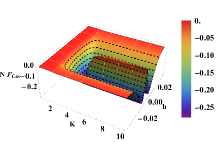
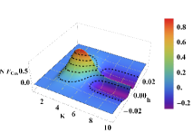
Figure 1: If $K_{a}>0$ the Casimir force is attractive (the corresponding function is negative). In the opposite case - with $K_{a}<0$, the force can be both attractive and repulsive, depending on $K$ and $h$. The force is always symmetric with respect of the sign of the external magnetic field $h$. In the current figure the left panel shows the behavior of the Casimir force for $N=100$ with $K_{a}=3$. The right panel depicts the behavior of the Casimir for with again $N=100$ but for $K_{a}=-3$. The behavior of the force is shown as a function of $K$ and $h$.

The behavior of the Casimir force as a function of $K$, $K_{a}$ and $h$ for $N=100$ and $K_{a}=\pm 3$ is shown in Fig. 1.

Let us now consider the behavior of the force in the scaling regime. On general grounds we expect that the scaling function of the Casimir force $X_{\rm Cas}(x_{t},x_{a},x_{h})$ is

$$\beta F_{\rm Cas}^{\rm(db)}(N,K,h)=\frac{1}{N}X_{\rm Cas}^{\rm(db)}(x_{t},K_{a},x_{h}).$$ (33)

From Eq. (24), and Eqs. (31) – (33) one derives the corresponding explicit expressions

$$X_{\rm Cas}^{\rm(db)}(x_{t},K_{a},x_{h})=-\frac{\sqrt{x_{h}^{2}+x_{t}^{2}}}{r(x_{t},K_{a},x_{h})\exp\left(\sqrt{x_{h}^{2}+x_{t}^{2}}\right)+1},$$ (34)

where

$$r(x_{t},K_{a},x_{h})=\frac{\sqrt{x_{h}^{2}+x_{t}^{2}}+x_{t}\exp(-2K_{a})}{\sqrt{x_{h}^{2}+x_{t}^{2}}-x_{t}\exp(-2K_{a})}.$$ (35)

Obviously, if $r(x_{t},K_{a},x_{h})>0$ one has $X_{\rm Cas}(x_{t},K_{a},x_{h})<0$. Furthermore, $X_{\rm Cas}(x_{t},K_{a},x_{h})$ decays exponentially when $x_{h}^{2}+x_{t}^{2}\gg 1$.

The behavior of the scaling function $X_{\rm Cas}^{\rm(db)}(x_{t},K_{a},x_{h})$ of the Casimir force are visualized in Fig. 2. We observe, that the force is symmetric with respect to the sign of $x_{h}$, as must be the case.

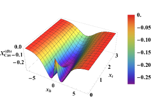
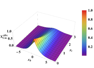
Figure 2: On the left panel: The behavior of the scaling function $X_{\rm Cas}^{\rm(db)}(x_{t},K_{a},x_{h})$ of the Casimir force as a function of the scaling variables $x_{t}$ and $x_{h}$ for $K_{a}=3$. We observe that the function is negative for all values of $x_{t}$ and $x_{h}$, i.e., the force is attractive. On the right panel: The behavior of the function $X_{\rm Cas}^{\rm(db)}(x_{t},K_{a},x_{h})$ for $K_{a}=-3$. We observe that the force is repulsive.

5 On the Behavior of the Model in Canonical Ensemble

In the canonical ensemble the total magnetization $M$ of the chain is fixed. This constrain can be expressed by using an integral presentation of the Kronecker delta-function

$$\delta[S,M]=\frac{1}{2\pi}\int_{-\pi}^{+\pi}e^{i(S-M)\phi}d\phi,\quad S=\sum_{i=1}^{N}S_{i},\quad S,M\in\mathbb{Z}.$$ (36)

Then the canonical partition function is given by

$$Z^{\rm(db)}_{C}(N,K,K_{a},M)=\sum_{\{S_{i}\}_{\rm(db)}}e^{-\beta{\cal H}}\delta[S,M],\quad$$ (37)

where ${\cal H}$ is given by Eq. (8) with $J_{BC}=J_{a}$. Here the symbol $\{S_{i}\}_{\rm(db)}$ means that the set of spins obeys the boundary conditions with a defect bond. Further we have

$$Z^{(\rm db)}_{C}(N,K,K_{a},M) = \frac{1}{2\pi}\int_{-\pi}^{\pi}{e^{-iM\phi}\left[\sum_{\{S_{i}\}^{\rm(db)}}e^{-\beta{\cal H}+i\phi\sum_{i}S_{i}}\right]}d\phi$$ (38)

$$= \frac{1}{2\pi}\int_{-\pi}^{\pi}{e^{-iM\phi}}\;Z^{(\rm db)}_{\rm GC}(N,K,K_{a},i\phi)\,d\phi.$$

Using Eq. (19), as well as (Dantchev2024, , see there Eqs. (2.9) and (2.11)), one derives

$$Z^{(\rm db)}_{\rm GC}(N,K,K_{a},i\phi)=2\left[\sqrt{2\sinh(2K)}\right]^{N-1}$$ (39)

$$\times\bigg{\{}e^{K_{a}}\cos(\phi)T_{N-1}\bigg{(}\tilde{z}(K,\phi\bigg{)}+\frac{e^{-(K_{a}+K)}-e^{K+K_{a}}\sinh^{2}(\phi)}{\sqrt{2\sinh(2K)}}U_{N-2}\bigg{(}\tilde{z}(K,\phi)\bigg{)}\bigg{\}},$$

where

$$\tilde{z}(K,\phi)\equiv z(K,i\phi)=\frac{e^{K}\cos(\phi)}{\sqrt{2\sinh(2K)}},\quad K>0,\quad\phi\in[-\pi,\pi].$$ (40)

Plugging Eq. (39) into Eq. (38) after using the properties of the Chebyshev’s polynomials (GR, , 8.941.1-8.941.3) it can be shown that

$$Z^{\rm(db)}_{C}(N,K,K_{a},M) = \left[\sqrt{2\sinh(2K)}\right]^{N}\bigg{\{}\bigg{[}e^{K_{a}-K}-\frac{\sinh(K_{a}+K)}{\sinh(2K)}\bigg{]}{\rm D}\left(N,M;e^{-4K}\right)$$ (41)

$$+\frac{1}{2}e^{K-K_{a}}\bigg{[}\frac{e^{2K_{a}}-e^{-2K}}{\sinh(2K)}\bigg{]}{\rm I}(N,M,e^{-4K})\bigg{\}}.$$

Here

$${\rm I}(N,M,z):=\frac{4}{\pi}\int_{0}^{\pi/2}\cos(Mx)\;T_{N}\left(\frac{\cos(x)}{\sqrt{1-z}}\right)dx,$$ (42)

and

$${\rm D}\left(N,M;z\right)=\frac{4}{\pi}\int_{0}^{\pi/2}\cos(Mx)\frac{\cos(x)}{\sqrt{1-z}}U_{N-1}\left(\frac{\cos(x)}{\sqrt{1-z}}\right)\,dx.$$ (43)

As shown in Ref. Dantchev2023b and Dantchev2024 , the above integrals can be expressed in terms of the Gauss hypergeometric functions. The results are

$${\rm I}(N,M,z)=Nz(1-z)^{-N/2}\;_{2}F_{1}\left(\frac{1}{2}(M-N+2),\frac{1}{2}(-M-N+2);2,z\right),$$ (44)

and

$${\rm D}(N,M,z)=(1-z)^{-N/2}z\;\bigg{\{}N\;_{2}F_{1}\left(\frac{1}{2}(M-N+2),\frac{1}{2}(-M-N+2);2,z\right)+$$

$$2(z^{-1}-1)\;_{2}F_{1}\left(\frac{1}{2}(M-N+2),\frac{1}{2}(-M-N+2);1,z\right)\bigg{\}}.$$ (45)

Thus, we have derived in an exact explicit form the partition function of the one-dimensional Ising model with fixed magnetization $M$ possessing a defect bond $K_{a}$. Now we pass to its scaling behavior. Using the asymptotic expansion (Dantchev2023b, , Eq. (D.6)), which in the current notations reads

$$_{2}F_{1}(\frac{1}{2}(Nm-N+2), \frac{1}{2}(-Nm-N+2);\gamma;e^{-4K})\simeq$$ (46)

$$(\gamma-1)!\left(\frac{1}{4}\sqrt{1-m^{2}}\,x_{t}\right)^{1-\gamma}\left[I_{\gamma-1}\left(\frac{1}{2}\sqrt{1-m^{2}}\,x_{t}\right)+O(N^{-1})\right],$$

from Eq. (41), and Eqs. (44), (5), we obtain

$$e^{-KN} Z^{(D)}_{C}(N,K,K_{a},M)=$$

$${\cal A}(K,K_{a})\frac{I_{1}\left(\frac{1}{2}\sqrt{1-m^{2}}\,x_{t}\right)}{\sqrt{1-m^{2}}}+{\cal B}(K,K_{a})I_{0}\left(\frac{1}{2}\sqrt{1-m^{2}}\,x_{t}\right),$$

where, for $K\gg 1$:

$${\cal A}=2e^{-2K}\bigg{\{}\bigg{[}e^{K_{a}-K}-\frac{\sinh(K_{a}+K)}{\sinh(2K)}\bigg{]}+\frac{1}{2}e^{-K_{a}}\bigg{[}\frac{e^{2K_{a}}-e^{-2K}}{e^{-K}\sinh(2K)}\bigg{]}\bigg{\}}\underset{K\gg 1}{\simeq}2e^{K_{a}-3K}.$$ (48)

and

$${\cal B}=2\bigg{[}e^{K_{a}-K}-\frac{\sinh(K_{a}+K)}{\sinh(2K)}\bigg{]}\underset{K\gg 1}{\simeq}2e^{-K_{a}-3K}.$$ (49)

6 Behavior of the Helmholtz Force in Ising Chain with Defect Bond

Based on Eqs. (41) – (5) we are ready to derive the behavior of the Helmholtz force defined in Eqs. (6) – (7). The only additional information we still need is the behavior of the bulk Helmholtz free energy density. It is, see Ref. Dantchev2023b and Ref. Dantchev2024

$$\beta a_{b}(K,m) =K+\frac{1}{2}\ln(1-m^{2})$$ (50)

$$-\ln\left[1+\sqrt{m^{2}+e^{4K}(1-m^{2})}\right]+\;m\sinh^{-1}\left(\frac{e^{-2K}m}{\sqrt{1-m^{2}}}\right).$$

The behavior of the Helmholtz force is shown in Figs. 3 and 4 . In Fig. 3 the force is visualized as a function of $K$. The left panel of the figure shows the behavior of the force for magnetization $m=0.1$ and for the three limiting cases of the values of the coupling constant: $K_{a}=K$, when our system is equivalent to the one with periodic boundary conditions, for $K_{a}=-K$ when it represents a system under antiperiodic boundary conditions, and with $K_{a}=0$ when it turns into a system with Dirichlet boundary conditions. We see that the obtained curves, calculated for $N=300$, agree completely with the ones reported in Refs. DR2022 ; Dantchev2023b ; Dantchev2024 . The right panel of Fig. 3 shows the behavior of the Helmholtz force for $N=100$ with the values of $K_{a}$ fixed ate $K_{a}=\pm 3$. We observe that for moderate values of $K$ the behavior of the force essentially differ in the two sub-case having, however, the same asymptotic for large and small values of $K$.

t]  

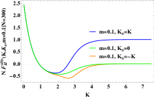
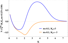
Figure 3: If $K_{a}>0$ the Helmholtz force is similar to the corresponding result for PBC’s - see Refs. DR2022 ; Dantchev2023b ; Dantchev2024 . In the opposite case - with $K_{a}<0$, the force resembles the one for ABC’s - see Refs. Dantchev2023b ; Dantchev2024 . The force is always symmetric with respect of the sign of $M$. In the current figure the left panel shows the behavior of the Helmholtz force for $N=100$ with $K_{a}=\pm K$. The right panel depicts the behavior of the force with again $N=100$ but for $K_{a}=\pm 3$.

The Helmholtz force as a function of $K_{a}$ for two pairs of fixed values of $m$ and $K$ is depicted in Fig. 4 as a function of $K_{a}$. The left panel demonstrates the influence of $K$ when $m$ is fixed, while the right panel show the complimentary case - the role of the value of $m$ when $K$ is fixed.

t]  

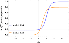
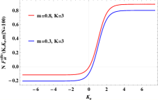
Figure 4: The Helmholtz force as a function of $K_{a}$ for two fixed pairs of values of $m$ and $K$. The left panel demonstrates the influence of $K$ for a fixed value of $m=0.1$, while the right panel shows the role of $m$ for a fixed value of $K=3$. We observe that for large values of $K$ the force is very small for negative values of $K_{a}$. For moderate values of $K$ (say $K=3$) the force is a negative constant for negative values of $K_{a}$, and positive for large values of $K_{a}$.

7 Discussion and concluding remarks

In the current article we have presented a brief review of some of the fluctuation induced forces. This have been done in Sec. 1. We commented on the QED and critical Casimir force, as well as on the newly introduced Helmholtz force. Some theoretical questions of practical application in nano- and micro-world have been outlined and discussed. Then the behavior of the critical Casimir and Helmholtz forces have been considered on the example of the one-dimensional Ising model in grand canonical and in the canonical statistical mechanical ensembles. The model is with one defect bond and is defined in Sec. 2.

The behavior of the model in grand canonical ensemble is studied in Sec. 3. The main result there is the exact expression for the partition function of the model given in Eq. (19) and Eq. (20).

The behavior of the Casimir force is investigated in Sec. 4. The main results are visualized in Figs. 1 and 2.

• Fig. 1 shows the behavior of the force for general values of the basic two parameters of the model - the strength of the coupling constant $K$ and the external magnetic field $h$. The calculations are performed for $N=100$. We observe that when the defect bond $K_{a}$ is of a ferromagnetic type, see the left panel, force is attractive and symmetric, as expected, with respect to the sign of the external magnetic field.

• When the defect bond is of antiferromagnetic type. i.e., $K_{a}<0$ the behavior of the force is much more interesting in that it can be both attractive and repulsive - see the right panel of the figure.

• On the left panel of Fig. 2 it is shown the scaling function of the Casimir force $X_{\rm Cas}^{\rm(db)}(x_{t},K_{a}=3,x_{h})$, with the scaling variables $x_{t}$ and $x_{h}$ defined in Eq. (24). Since $K_{a}>0$ the behavior of the force is similar to that of the periodic boundary, conditions, i.e., the force is attractive.

• In the right panel of Fig. 2 the opposite case of $X_{\rm Cas}^{\rm(db)}(x_{t},K_{a}=-3,x_{h})$. As we see, with $K_{a}<0$ the force resembles the one for antiperiodic boundary conditions and is always repulsive.

The behavior of the model in the canonical ensemble is considered in Sec. 5. Again, the main result there is the explicit exact expression for the partition function of the model given in Eqs.(41) – (5). It is presented there in terms of the Gauss hypergeometric functions.

The behavior of the Helmholtz Force in Ising chain with defect bond is considered in Sec. 6. The basic results are depicted in Figs. 3 and 4.

• Fig. 3 represents the behavior of the Helmholtz force as a function of the coupling constant $K$. On the left panel few principal cases of the value of $K_{a}$, namely $K_{a}=K,K_{a}=-K$ and $K_{a}=0$ are shown. The value of the magnetization is fixed to $m=0.1$. We observe that the force can be both attractive and repulsive and coincides with the behavior of the system with periodic, antiperiodic and Dirichlet, boundary conditions, respectively.

• The right panel of Fig. 3 clearly shows that the precise value of $K_{a}$, with all other parameters kept the same, is important for the behavior of the force.

• Fig. 4 depicts the Helmholtz force as a function of $K_{a}$. We observe that for large values of $K$ the force is very small for negative values of $K_{a}$. The force changes sign for moderate values of $K$ (say $K=3$): it is attractive for negative values of $K_{a}$, and repulsive for large values of $K_{a}$.

We find that all significant results are consistent with the expectations of finite-size scaling theory BDT2000 .

The present article demonstrates that the behavior of the fluctuation induced forces crucially depend on the statistical ensemble in which they are defined and also on the presence of impurity in the system. These important issues have not been intensively studied yet.

Competing Interests This study was funded by the Bulgarian NSF via Grant No KP-06-H72/5.
The authors have no conflicts of interest to declare that are relevant to the content of this chapter.

Ethics Approval
Informed consent to publish was obtained from the individual participants of the article.

References

- (1) D. Dantchev, J. Rudnick, Phys. Rev. E 106, L042103 (2022). DOI 10.1103/PhysRevE.106.L042103. URL https://link.aps.org/doi/10.1103/PhysRevE.106.L042103
- (2) D. Dantchev, S. Dietrich, Physics Reports 1005, 1 (2023). DOI https://doi.org/10.1016/j.physrep.2022.12.004. URL https://www.sciencedirect.com/science/article/pii/S0370157322004070
- (3) A. Einstein, Annalen der Physik 327(3), 569 (1907). DOI 10.1002/andp.19073270311. URL http://dx.doi.org/10.1002/andp.19073270311
- (4) H.B. Casimir, Proc. K. Ned. Akad. Wet. 51, 793 (1948)
- (5) V.M. Mostepanenko, N.N. Trunov, The Casimir effect and its applications (Energoatomizdat, Moscow, 1990, in Russian; English version: Clarendon, New York, 1997)
- (6) M. Kardar, R. Golestanian, Rev. Mod. Phys. 71(4), 1233 (1999). DOI 10.1103/RevModPhys.71.1233
- (7) K.A. Milton, The Casimir Effect: Physical Manifestations of Zero-point Energy (World Scientific, Singapore, 2001)
- (8) M. Bordag, G.L. Klimchitskaya, U. Mohideen, V.M. Mostepanenko, Advances in the Casimir effect (Oxford University Press, Oxford, 2009)
- (9) K.A. Milton, J. Phys. A: Math. Gen. 37, R209 (2004)
- (10) C. Genet, A. Lambrecht, S. Reynaud, Eur. Phys. J. Special Topics 160, 183–193 (2008)
- (11) G.L. Klimchitskaya, U. Mohideen, V.M. Mostepanenko, Int. J. Mod. Phys. B 25, 171 (2011). DOI 10.1142/S0217979211057736
- (12) A.W. Rodriguez, F. Capasso, S.G. Johnson, Nature Photonics 5, 211–221 (2011). DOI doi:10.1038/nphoton.2011.39
- (13) A. Farrokhabadi, N. Abadian, F. Kanjouri, M. Abadyan, Int. J. Mod. Phys. B 28(19), 1450129 (2014). DOI 10.1142/S021797921450129X. URL http://www.worldscientific.com/doi/abs/10.1142/S021797921450129X
- (14) A. Farrokhabadi, J. Mokhtari, R. Rach, M. Abadyan, Int. J. Mod. Phys. B 29(02), 1450245 (2015). DOI 10.1142/S0217979214502452. URL http://www.worldscientific.com/doi/abs/10.1142/S0217979214502452
- (15) E.M. Lifshitz, Sov. Phys. 2, 73; (1956). Zhur. Eksptl. i Teoret. Fiz.29, 94–110 (1955) (In Russian)
- (16) E.M.L. L. E. Dzyaloshinskii, L.P. Pitaevskii, Adv. Phys. 10, 165 (1961)
- (17) J. Mahanty, B.W. Ninham, Dispersion Forces (Academic, New York, 1976)
- (18) V.A. Parsegian, Van der Waals Forces (Cambridge University Press, New York, 2006)
- (19) I.E. Dzyaloshinskii, E.M. Lifshitz, L.P. Pitaevskii, Sov. Phys. Usp. 4, 153 (1961). In Russian: Usp. Fiz. Nauk 73, 381 (1961).
- (20) S. Dietrich, in Phase Transitions and Critical Phenomena, vol. 12, ed. by C. Domb, J.L. Lebowitz (Academic, New York, 1988), pp. 1–218
- (21) J.N. Munday, F. Capasso, V.A. Parsegian, Nature 457(7226), 170 (2009). URL http://dx.doi.org/10.1038/nature07610
- (22) M.E. Fisher, P.G. de Gennes, C. R. Seances Acad. Sci. Paris Ser. B 287, 207 (1978)
- (23) M. Krech, The Casimir Effect in Critical Systems (World Scientific, Singapore, 1994)
- (24) J.G. Brankov, D.M. Dantchev, N.S. Tonchev, The Theory of Critical Phenomena in Finite-Size Systems - Scaling and Quantum Effects (World Scientific, Singapore, 2000)
- (25) A. Maciołek, S. Dietrich, Rev. Mod. Phys. 90, 045001 (2018). DOI 10.1103/RevModPhys.90.045001. URL https://link.aps.org/doi/10.1103/RevModPhys.90.045001
- (26) A. Gambassi, S. Dietrich, DOI 10.48550/ARXIV.2312.15482
- (27) D.M. Dantchev, N.S. Tonchev, J. Rudnick, Annals of Physics 459, 169533. DOI https://doi.org/10.1016/j.aop.2023.169533. URL https://www.sciencedirect.com/science/article/pii/S0003491623003354
- (28) R.J. Baxter, Exactly Solved Models in Statistical Mechanics (Academic, London, 1982)
- (29) K. Huang, Statistical Mechanics, 2nd edn. (John Wiley & Sons, New York, 1987)
- (30) M. Kardar, Statistical Physics of Fields (Cambridge University Press, Cambridge, 2007)
- (31) R.K. Pathria, P.D. Beale, Statistical Mechanics, 3rd edn. (Elsevier, Amsterdam, 2011)
- (32) B. Liebchen, H. Löwen, The Journal of Chemical Physics 150(6), 061102 (2019). DOI 10.1063/1.5082284. URL https://doi.org/10.1063/1.5082284
- (33) D.M. Dantchev, N.S. Tonchev, J. Rudnick, DOI 10.48550/ARXIV.2402.04459
- (34) I.S. Gradshteyn, I.H. Ryzhik, Table of Integrals, Series, and Products (Academic, New York, 2007)