Graph Protection under Multiple Simultaneous Attacks: A Heuristic Approach

Abstract

This work focuses on developing an effective meta-heuristic approach to protect against simultaneous attacks on nodes of a network modeled using a graph. Specifically, we focus on the $k$-strong Roman domination problem, a generalization of the well-known Roman domination problem on graphs. This general problem is about assigning integer weights to nodes that represent the number of field armies stationed at each node in order to satisfy the protection constraints while minimizing the total weights. These constraints concern the protection of a graph against any simultaneous attack consisting of $k\in\mathbb{N}$ nodes. An attack is considered repelled if each node labeled 0 can be defended by borrowing an army from one of its neighboring nodes, ensuring that the neighbor retains at least one army for self-defense. The $k$-SRD problem has practical applications in various areas, such as developing counter-terrorism strategies or managing supply chain disruptions. The solution to this problem is notoriously difficult to find, as even checking the feasibility of the proposed solution requires an exponential number of steps. We propose a variable neighborhood search algorithm in which the feasibility of the solution is checked by introducing the concept of quasi-feasibility, which is realized by careful sampling within the set of all possible attacks. Extensive experimental evaluations show the scalability and robustness of the proposed approach compared to the two exact approaches from the literature. Experiments are conducted with random networks from the literature and newly introduced random wireless networks as well as with real-world networks. A practical application scenario, using real-world networks, involves applying our approach to graphs extracted from GeoJSON files containing geographic features of hundreds of cities or larger regions.

1]marko.djukanovic@pmf.unibl.org

2]stefan.kapunac@matf.bg.ac.rs

3]aleksandar.kartelj@matf.bg.ac.rs

4]dragan.matic@pmf.unibl.org

1 Introduction

Domination problems on graphs represent one of the most frequently solved class of problems in the field of computer science, thoroughly investigated theoretically as well as computationally (see surveys [9, 18, 11] providing an overview on theoretical results, and [25, 5] for an overview on algorithmic results). Given an input graph $G=(V,E)$, the minimum domination problem asks for finding a minimum cardinalty subset $S$ of nodes of graph $G$, so that any node from $V$ either belongs to $S$ or is adjacent to at least one node from $S$. Many variants of the minimum domination problem are proposed, corresponding to a a wide range of practical applications, e.g. in telecommunications [3], scheduling problems [32], and detecting RNA motifs in biological networks. Many of them are related to well-known facility location problems [14]. In the course of this work, we pay particular attention to a problem belonging to class of the Roman domination problems (RDPs); these problems are thoroughly solved in the literature from both perspectives, theoretically and practically, see [7, 10]. The basic RDP seeks for a positive integer node labeling with the minimum cumulative weight over all nodes of a graph, such that every node labeled with 0 must have at least one neighboring node labeled with 2. This problem can be seen by ensuring a network with minimum cost for each possible individual (node) attack. RDP and its variants are well solved practically in the literature, e.g. by means of an integer linear program [31, 4], a genetic algorithm [23], a variable neighborhood search [20], etc. Practical applications of RDP have been found in the search for an optimal military strategy [19], network design of server placements [29], to name a few.

In this paper, we study a practically motivated variant of RDP where $k\in\mathbb{N},k\geq 2$ attacks occur simultaneously on the nodes of a graph; the problem is called k-Strong Roman domination ($k$-SRD) problem [24]. It is similar to a basic RDP, but instead of a single node being attacked, any combination of $k\geq 2$ nodes can be attacked, and all of these attacks must be defended against by the respective neighboring nodes. In reality, a scenario may arise where defenders need to be prepared for multiple simultaneous attacks in order to secure more than one site at a time, e.g., when planning counter-terrorism strategies. Other applications of this problem can be found in disaster relief or supply chain disruptions [24]. Verifying the feasibility of the proposed solution requires an exponential number of steps. To develop an efficient algorithm, we have defined the concept of $k$-SRD quasi-feasibility. We highlight another optimization problem that also considers multiple simultaneous attacks on graphs, but under different constraints; it is the strong Roman domination problem [2].

Concerning the literature on the $k$-SRD problem, there are, to our knowledge, two papers in the existing literature. One of the papers deals with theoretical aspects of the problem [28]. The second paper [24] examines the problem from a practical perspective. In this study, the authors propose two exact algorithms: an integer linear programming model and, based on it, a Benders-based decomposition technique; the latter approach slightly outperforms the former in terms of the number of optimally solved instances. The number of variables of the ILP model is $O\left(\binom{n}{k}\cdot n^{2}\right)$, while the number of constraints is $O\left(\binom{n}{k}\cdot n\right)$; thus, the size of the model grows exponentially with the number of variables and constraints as the instance size increases. Therefore, the model requires enormous computational resources to be constructed for large problem instances. As an alternative, a Benders-based decomposition approach was proposed in the same paper. Besides all these facts, we noticed some other problems. First, the approaches were only tested on a set of randomly generated instances of limited size with an instance size of up to 30 (nodes) and up to $k=5$. Therefore, these graph sizes can hardly model a realistic attack scenario, indicating potential problems with the scalability of the approaches. Moreover, random graphs may be unsuitable for modelling real-world use cases. Secondly, as already mentioned, exact approaches are usually only suitable to a limited extent for solving such difficult problems. A reasonable way is to consider approximation search methods, and one of them is certainly meta-heuristics. The contributions of this work are as follows.

• To solve the $k$-SRD problem on larger instances and thus more realistic graphs, we propose a variable neighborhood search (VNS) approach [27], the first known heuristic approach to solve this problem. This method is equipped with an efficient procedure that verifies solution feasibility based on the introduced concept of quasi-feasibility. For that purpose, two strategies are used to defend against a set of (predefined) attacks: a deterministic one, which is used when the number of attacks is rather small, and a more robust stochastic one, which is based on a roulette selection to choose neighboring nodes as defenders of the attacked nodes.

• A greedy approach was proposed to quickly find a feasible solution of adequate quality. This method also supports the VNS approach as the solution derived by the greedy approach serves as a starting point for the VNS.

• We extend the current set of random instances by creating additional sets of instances with different distributions. These are constructed using the model Unit disc model [8], which generates random geometric graphs commonly used to model wireless ad hoc networks. The purpose of these instances is to test the robustness of the literature approaches together with the two proposed approaches under more realistic graphs of different densities.

• A new application scenario for the $k$-SRD problem has been provided using a set of real instances. More specifically, this use case is about applying the $k$-SRD solution to graphs representing cities divided into districts or regions. The task is to select suitable locations for the construction of fire stations and to place a number of fire trucks to ensure the extinguishing of fire disasters that may occur simultaneously at $k$ locations.

• Our VNS approach shows its effectiveness by achieving solutions that are close to (or equal to) the quality of known optimal solutions for small instances. For medium to large instances, the two exact approaches from the literature are far from being applicable (except partially for the case of small $k=2$), since it is impossible to construct the model within a reasonable memory consumption or the given time limit. This was not the case with our VNS, which has greater robustness compared to the exact methods. Moreover, VNS significantly improves the initial solutions generated by our greedy approach, as demonstrated by appropriate statistical tests.

1.1 Problem definition

Let $G=(V(G),E(G))$ be a simple undirected graph where $V(G)$ and $E(G)$ represent its nodes and edges, respectively. Let $n=|V(G)|$ be the number of nodes of the graph $G$, also called the size of the graph. With $d(v),v\in V(G)$ we denote the degree of the node $v$, and with $\Delta(G)=\max\{d(v)\mid v\in V(G)\}$ the maximum degree of the graph $G$. Let $f\colon V(G)\mapsto\mathbb{N}_{0}$ map the nodes of the graph to the numbers (of armies) and let $\omega(f,G)=\sum_{v\in V(G)}f(v)$ be the sum of these numbers for the entire $G$. (We always consider $n\geqslant k$ throughout the paper; otherwise we arrive at the trivial solution of the problem.)

For a graph $G$, let $P:=\{v_{1},v_{2},\ldots,v_{k}\}$, $v_{1},v_{2},\ldots,v_{k}\in V(G)$ denote an attack pattern, or simply, the set of nodes under attack. Note that there are $\binom{|V(G)|}{k}$ different attacks for the graph $G$ and the fixed value of $k$. Therefore, the number of attacks grows exponentially in the instance size ($n$). Let $\mathcal{P}(G):=\{P_{1},\ldots,P_{\binom{|V(G)|}{k}}\}$ be the set of enumerated attacks for graph $G$.

A function $f:V(G)\mapsto\{0,1,\ldots,\min(\Delta(G),k)+1\}$ is a proper $k$-SRD function if each attack $P\in\mathcal{P}(G)$ is defended, where the defense rules are as follows:

• Nodes labeled with $f(v)=1$ can defend only themselves.

• Nodes labeled with $f(v)\geq 2$ can defend themselves and, in addition, at most $f(v)-1$ attacked neighboring nodes labeled with 0.

• Nodes labeled with 0 that are under attack $P$ must be defended by at least one of their neighboring nodes.

The problem of $k$-SRD on the graph $G$ seeks for a valid $k$-SRD function $f$ on $G$ with minimum $\omega(f)$, called $k$-SRD number $\gamma_{k-SRD}(G)$, i.e. $\gamma_{k-SRD}(G):=\min\{\omega(f)\mid f\text{ is a proper }k\text{-SRD function on the graph }G\}$. Such a $k$-SRD function for which $\gamma_{k-SRD}(G)$ is reached is simply called $\gamma_{k-SRD}$ function. Figure 1 depicts a graph and an attack for which the defense strategy is given. Note that the solution $f$ is not a $3$-SRD function, since three more attacks need to be defended. For example, an attack $P=\{A,B,D\}$ could not be defended with $f$. An optimal strategy for defending against all attacks on any three nodes of the graph is shown in Figure 2.

Figure 1: 3-SRD problem: An attack $P=\{A,B,E\}$ (filled in gray) can be defended by a function $f$ provided with $f(D)=f(A)=f(B)=0$, $f(C)=3$ and $f(E)=1$ with a $\omega(f)=4$. But, the attack $P=\{A,B,D\}$ cannot.

Figure 2: 3-SRD problem: An optimal strategy for the $3$-SRD function $f$. It comes with $\omega(f)=5$.

The assignment of a number $c\in\mathbb{N}_{0}$ to a node can be seen as determining the number of field armies (FAs) at that node. The aspect of protecting an undefended node – which has no FAs – can be interpreted as moving an FA that is at a neighboring location to that (unprotected) location. Some direct properties of a valid $k$-SRD function are given as follows. By assigning the value 1 to all nodes in $G$, all nodes are considered safe for any attack of $\mathcal{P}$, so that we obtain a trivially valid $k$-SRD function on any graph $G$ and thus an upper bound for the $\gamma_{k-SRD}$-number of a graph of size $n$. All label assignments with only positive values are therefore considered trivially protected. This means that only assignments that contain at least one node labeled with 0 are of interest to us.

The rest of the paper is structured as follows. In Section 2, details are given about the designed VNS approach to solve the $k$-SRD problem. In addition, a greedy approach for the $k$-SRD problem is presented. Section 3 provides a thorough experimental evaluation between our two heuristic approaches and the two exact literature approaches. Section 4 describes a use case of the $k$-SRD problem using instances extracted from spatial data of GeoJSON files. This paper concludes with section 5 and an outlook on future work.

2 Variable neighborhood search for $k$-SRD problem

Variable neighborhood search is a powerful single-point search meta-heuristic developed by Mladenović and Hansen [27]. It has been applied to numerous difficult computational problems from various fields, such as scheduling [33, 1], allocation problems [16], routing [21, 17], bioinformatics problems [6, 12], domination problems [20, 22] and many others.

The main idea of VNS is to use a set of different neighborhood structures with increased cardinality around a solution to avoid the search getting stuck in local optima. When the algorithm makes no progress, a new (usually increasingly larger) neighborhood structure is placed around the current solution. Various versions of the VNS are known in the literature, such as the variable neighborhood decomposition [15], the skewed VNS [34], the general VNS [26], etc. The schematic of the basic VNS is shown in Algorithm 1.

1:Input: problem instance $I$, $r_{\min},r_{\max}>0$, a set of neighborhood structures $\mathcal{N}_{r_{\min}},\ldots,\mathcal{N}_{r_{\max}}$, (fitness) function $f$

2:Ouput: solution $s$

3:$s\leftarrow\texttt{generate\_initial\_solution}(I)$

4:$s_{best}\leftarrow s$

5:while !(any of termination criteron is met) do

6:     $r\leftarrow r_{\min}$

7:     while $r\leq r_{\max}$ do

8:         $s^{\prime}\leftarrow\texttt{shake}(s,\mathcal{N}_{r})$

9:         $s^{\prime\prime}\leftarrow\texttt{local\_search}(s^{\prime})$

10:         $s_{best},r\leftarrow\texttt{acceptance\_criterion}(s_{best},s^{\prime\prime},r)$

11:     end while

12:end while

13:return $s_{best}$

Algorithm 1 The basic VNS framework

The algorithm first initializes a starting solution $s_{best}$, usually randomly, or in a more sophisticated way, e.g. using a greedy procedure or another meta-heuristic that quickly provides a solution of reasonable quality. Subsequently, the main loop is initiated by executing basic VNS iterations as long as one of the termination conditions is not met: allowed time limit, allowed number of VNS iterations exceeded, number of iterations reached without any improvement, etc. A single VNS iteration consists of entering the inner loop in which the neighboring structures are systematically examined, starting with the smallest, i.e. $r\leftarrow r_{\min}$. In each iteration, the operator shake() is executed on the solution $s$ around the $r$-th neighboring structure which returns a modified solution $s^{\prime}$. This solution is potentially improved by a local search procedure local_search(). Then, based on the function acceptance_criterion(), this new solution $s^{\prime\prime}$ is either accepted or not for a new incumbent, which changes the value of $r$. (Usually, $r\leftarrow r_{\min}$ when $s^{\prime\prime}$ is accepted.) The inner loop runs until $r$ no longer reaches $r_{\max}$, i.e. when all neighborhood structures around $s_{best}$ have been examined.

The rest of this section is devoted to the details of the design of an efficient VNS for solving the $k$-SRD problem.

2.1 Predefined attacks and the concept of quasi-feasibility

Before delving into the specifics of the primary procedures that form the core of the main VNS, it is crucial to acknowledge the inherent difficulty in verifying the feasibility of a single solution for this problem in general. This challenge is primarily attributed to the exponentially increasing number of attacks to be verified as the instance size grows. Consequently, we introduce two fundamental concepts designed to address this issue: a set of predefined attacks and the quasi-feasibility. Ultimately, these concepts enable us to tackle large-sized instances from a practical standpoint.

2.1.1 Predefined attacks

We separate sets of attacks to two groups, both related to the concept of quasi-feasibility in general case, although exact feasibility can be reached for the cases of small to medium-sized instances:

• Intensive attacks, labeled by intense_attacks. These attacks are employed to assess the more confident quasi-feasibility of the current solution.

• Lightweight attacks labeled by lightweight_attacks. As explained in the subsequent paragraphs attacks of this type serve in the local search procedure to access the concept of relaxed quasi-feasibility.

The bound on the number of attacks is parameter comb_take_all_bound. In case $\binom{n}{k}<comb\_take\_all\_bound$, we utilize all possible $k$-attacks $\mathcal{P}$ for intense_attacks as well as for lightweight_attacks. Otherwise, we generate a subset $\mathcal{P}^{\prime}\subseteq\mathcal{P}$ of attacks in the following way. First, for each node $v$, the set $N_{l}^{v}$ consists of all nodes which are at the distance of at most $l$ from $v$. Given a set of nodes $s$ and $k$, by comb($s,k$) we simply denote the set of all $k$-combinations of set $s,|s|\geq k$. Further, for fixed node $v$, we generate the set of intense_attacks as the union of $comb(N_{3}^{v},k)$ across each node $v$. We chose $l=3$ for generating these attacks as it provides a good balance between the performance and good approximation of solution feasibility. In case that the size of intense_attacks does not exceed the value comb_take_all_bound, we set lightweight_attacks=intense_attacks, otherwise lightweight_attacks is obtained as the union of $comb(N_{1}(v),k)$ over all $v$.

2.1.2 The concept of quasi-feasibility

The concept of quasi-feasibility enhances tractability of verifying solution feasibility by focusing on a predefined set of attacks (intense_attacks) instead of verifying exponentially many attacks (all possible attacks). In practical terms, this entails replacing an exponential-time exact feasibility verification with a semi-decidable polynomial verification algorithm. (Semi-decidable in the sense that if the procedure yields a negative answer, the solution is indeed not feasible, and if the procedure yields a positive answer, the feasibility is not guaranteed to be feasible.) Specifically, for each predefined attack in the set intense_attacks, we assess whether the attack can be successfully defended according to the problem definition. If any attack proves to be undefended by our strategy, the solution is considered infeasible; otherwise, it is considered quasi or (weakly) feasible. The essential steps for verifying whether a specific attack can be successfully defended are outlined in Algorithm 2.

1:Input: solution $s$, $G=(V,E)$, $k$, attack, $cutoff>0$, $tries>0$

2:Output: a pair attack_defended, defending_nodes

3:$all\_alternatives,reduced\_attack\leftarrow\emptyset$

4:for $v\in attack$ do

5:    if $s[v]>0$ then

6:        add $v$ to defending_nodes

7:        continue

8:    end if

9:    $alternatives\leftarrow$ the set of all neighbors of $v$ that can defend it

10:    if $alternatives=\emptyset$ then

11:        return $False,\emptyset$

12:    end if

13:    add $v$ to $reduced\_attack$

14:    $all\_alternatives\leftarrow all\_alternatives\times alternatives$

15:end for

16:if $|all\_alternatives|<cutoff$ then

17:    return determinitic_defense($all\_alternatives,reduced\_attack,defending\_nodes$)

18:else

19:    return roulette_defense($reduced\_attack,defending\_nodes,tries$)

20:end if

Algorithm 2 Procedure is_attack_defended()

We have designed two defense strategies aimed at protecting nodes within the specified set of attacks: a deterministic strategy and a probabilistic one, outlined in Algorithms 6 and 7, respectively, see A for more details. The choice between these strategies is made based on the number of potential alternative protectors for all undefended nodes and the parameter cutoff. If the number of all alternatives is relatively small, we can afford to explore all combinations for defenders. Otherwise, we employ a roulette selection of protector nodes, i.e., nodes that have a greater chance of being selected as protectors for the current node. Since this probabilistic strategy may not succeed every time, we execute it multiple times controlled by the parameter $tries>0$.

The core procedure, called quasi_infeasibility() (Algorithm 3), for each attack $h\in intense\_attacks$ executes the function is_attack_defended() given in Algorithm 2. In case no valid defense is found, the counter that keeps track of the number of non-defended attacks is incremented, which is, at the end, returned by the procedure.

1:Input: solution $s$, $G=(V,E)$, $k$, attacks, $cutoff>0$, $tries>0$

2:Output: non_defended_count, coverage_info

3:$non\_defended\_count\leftarrow 0$

4:$coverage\_info\leftarrow\emptyset$

5:for $attack\in attacks$ do

6:    $defended,defending\_nodes\leftarrow$ is_attack_defended($s$, $G$, $k$, $attack$, $cutoff$, $tries$)

7:    if $defended$ then

8:        update_coverage_info($defending\_nodes$, $attack$)

9:    else

10:        $non\_defended\_count\leftarrow non\_defended\_count+1$

11:    end if

12:end for

Algorithm 3 Procedure quasi_infeasibility()

2.2 Initialization: a greedy approach

To initialize a feasible solution, we have devised an efficient greedy approach based on the principle of covering nodes of a graph. In the following section, we provide a detailed description of our greedy approach, pseudo-coded in Algorithm 4.

Initially, all nodes are assigned a label 0, represented as the solution $s=[0,\ldots,0]$ and the coverage $\emph{covered}=\emptyset$ which keeps nodes that are already protected under any attack. In each iteration, the algorithm decides which node to label based on a greedy criterion $g(\cdot)$. This criterion calculates, for each not-yet-processed node, the number of its neighboring nodes (counting also itself) still not included in the set covered. Among such nodes, the algorithm selects one with the highest $g$-value, denoted as $v^{\prime}$. Symbolically, the greedy value for a node $v\in V(G)\setminus\emph{covered}$ is determined by:

$$g(v)=|N[v]\setminus\emph{covered}|$$

If there are multiple nodes with equal $g$-value, we prioritize one not belonging to covered. The reasoning behind choosing this type of tie breaking is based on the following facts.

• If a node $v$ has, for example, $g(v)=3$ and $v$ itself is not covered, then it has to cover itself and two of its neighbors, so a total of $3$ FAs is sufficient.

• On the other hand, if the node $v$ is covered and has $g(v)=3$, that means it has three neighbors to cover and, as always, needs one FA for itself, resulting in $4$ FAs in total.

Then, a label $l_{v^{\prime}}=\min(k+1,g(v^{\prime})+I_{v^{\prime}\in covered})$ is assigned to $v^{\prime}$, that is $s[v^{\prime}]=l_{v^{\prime}}$, where $I$ is an indicator function. Consequently, all neighbors of $v^{\prime}$ immediately become covered – that is included in the set covered. The algorithm terminates when all nodes are covered.

1:Input: an instance $I$ of $k$-SRD problem, k

2:Output: solution $s$

3:$s\leftarrow[0,\ldots,0]$

4:$covered\leftarrow\emptyset$

5:while $covered\neq V(G)$ do

6:     $v^{\prime}\leftarrow\arg\max\{g(v)\mid v\in V(G)\setminus covered\}$ $\triangleright$ tie breaking - uncovered nodes go first

7:     $uncov_{v^{\prime}}\leftarrow N[v^{\prime}]\setminus covered$

8:     if $v^{\prime}\in uncov_{v^{\prime}}$ then

9:         $v^{\prime}\_not\_counted\leftarrow 0$

10:     else

11:         $v^{\prime}\_not\_counted\leftarrow 1$

12:     end if

13:     $s[v^{\prime}]\leftarrow\min(k+1,g(v^{\prime})+v^{\prime}\_not\_counted)$

14:     $covered\leftarrow covered\cup uncov_{v}$  

15:end while

Algorithm 4 Procedure greedy()

2.3 Shaking

This phase is in charge of diversifying the search process of the VNS algorithm. It is realized through the procedure $\texttt{shake}(s,r)$, where the input parameters consist of a solution $s$ and the $r$-th neighborhood structure $\mathcal{N}_{r}$. The output of this procedure yields a (mutated) solution $s^{\prime}$ generated in the following way. For a given solution $s$ that is to be shaked, we perform $r$ random increments and $r+1$ random decrements where decrement is performed on non-zero labels only. The choice of decrements is based on the roulette selection of the labels of solution $s$. For example, given a solution $s=[2,3,4,1]$ and $r=2$, after two random increments solution might be $s^{\prime}=[3,3,4,2]$ and after 3 decrements, it might be $s^{\prime}=[1,3,3,2]$. Therefore, $\omega(s)-\omega(s^{\prime})=1$.

2.4 Local search (LS)

The primary objective of local search is to intensify the exploration of solutions in the vicinity of a given solution $s$ with the aim of finding high-quality local optima. For the $k$-SRD problem, we have devised a suitable local search procedure guided by two key principles: ($i$) the quasi-swap principle; and ($ii$) the first-improvement strategy. As the LS can take considerable amount of time, feasibility of solutions generated through the LS process is verified in a relaxed fashion by using the set lightweight_attacks of predefined attacks.

The quasi-swap principle involves first shuffling the set of node pairs $(i,j)$, where $i<j$, before proceeding to the next step to eliminate any potential biases. Subsequently, for each node pair $(i,j)$, we apply partial-imputations of FAs from the set of 2-decomposition of the sum $s[i]+s[j]$. For instance, if $s[1]=2$, and $s[3]=3$, we construct the set of 2-decomposition for $2+3=5$: ${(0,5),(1,4),(3,2),(4,1),(5,0)}$. Then, for each 2-decomposition, replacing $s[i]$ and $s[j]$ with a respective component value is probed to generate a new solution candidates $\{(s[1]=0,s[3]=5),(s[1]=1,s[3]=4),...\}$. Afterwards, quasi-feasibility of a solution candidate (see Section 2.1.2) is verified, returning number of non-defended attacks (under the set of reduced, predefined attacks leveraged for an incremental fitness evaluation, see the next section). The solution is accepted as a new incumbent if the number of non-defended (reduced) attacks decreases. If no improvement is observed in that way, next 2-decomposition is probed to replace the current best solution’s components, and the process is repeated. If none of the 2-decomposition replacement yields an improvement over the incumbent solution, a different node pair $(i,j)$ is chosen, and the process is restarted.

If no improvement occurs with any node pair, the LS terminates unsuccessfully returning the same input solution $s$ along with its fitness score. Otherwise, if the number of non-defended attacks reaches 0 during the search, indicating the achievement of a (quasi-)feasible solution, the algorithm terminates successfully, returning the improved solution along with its new improved fitness score.

2.5 Fitness function

The fitness function $fitness$ for a $k$-SRD solution $s$ comprises two scores in the form of an ordered pair $fitness(s)=(\emph{quasi-infeasibility}(s),\emph{sum}(s))$, where:

• $\emph{quasi-infeasibility}(s)$ denotes the number of non-defended attacks for solution $s$, and

• $\emph{sum}(s)$ represents the sum of all elements in $s$.

For the LS, we have implemented a fast fitness score calculation method structured as follows. During each execution of quasi_infeasibility(), the coverage information is determined. This entails storing information within an appropriate data structure, referred to as coverage_info, when node $v$ is utilized as a defending node for an attack $h\in\textit{lightweight\_attacks}$. Leveraging this structure has proven to significantly accelerate the LS process, as it allows for rapid verification of some attacks in lightweight_attacks as protected for solutions $s^{\prime}$ in the vicinity of solution $s$.

2.6 The core VNS scheme for the $k$-SRD problem

We finally conclude the overall outline of the proposed VNS for $k$-SRD in Algorithm 5.

1:Input: an instance $I$ of $k$-SRD problem, $k,r_{\min},r_{\max},move_{prob},t_{\max},iter_{max},tries,cutoff$

2:Output: (possibly feasible) solution $s_{best}$

3:$intense\_attacks,lightweight\_attacks\leftarrow\texttt{generate\_attacks}(I,k)$ $\triangleright$ see Section 2.1

4:$s_{best}\leftarrow\texttt{greedy}(I,k)$ $\triangleright$ see Section 2.2

5:$iter\leftarrow 0$

6:$infeasibility_{s_{best}}\leftarrow\texttt{quasi\_infeasibility}(s_{best},intense\_attacks,cutoff,tries)$ $\triangleright$ see Section 2.1.2

7:$fitness_{s_{best}}\leftarrow(infeasibility_{s_{best}},sum(s_{best}))$

8:while $t_{passed}<t_{\max}$ and $iter<iter_{max}$ do

9:    for $r=r_{\min}\text{ to }r_{\max}$ do

10:        $iter\leftarrow iter+1$

11:        $s^{\prime}\leftarrow\texttt{Shake}(s_{best},r)$ $\triangleright$ see Section 2.3

12:        $s^{\prime},fitness_{s^{\prime}}\leftarrow\texttt{LS}(s^{\prime},lightweight\_attacks,tries)$ $\triangleright$ see Section 2.4

13:        if $fitness_{s^{\prime}}<fitness_{s_{best}}$ or ($fitness_{s^{\prime}}=fitness_{s_{best}}$ and $move_{prob}<u\in\mathcal{U}(0,1)$) then

14:           $intense\_infeasibility_{s^{\prime}}\leftarrow\texttt{quasi\_infeasibility}(s^{\prime},intense\_attacks,cutoff,tries)$

15:           if $intense\_infeasibility_{s^{\prime}}=0$ then $\triangleright$ solution is quasi-feasible

16:               $s_{best}\leftarrow s^{\prime}$

17:               $fitness_{s_{best}}\leftarrow(intense\_infeasibility_{s^{\prime}},sum(s^{\prime}))$

18:               break

19:           end if

20:        end if

21:    end for

22:end while

Algorithm 5 VNS algorithm for the $k$-SRD problem

In the first line of Algorithm 5, the tasks outlined in Section 2.1 are executed. Specifically, two distinct types of attacks, denoted as $intense\_attacks$ and $lightweight\_attacks$, are generated. Subsequently, the greedy algorithm from Section 2.2 is employed to produce an initial solution $s_{best}$. This solution is then subjected to verification via $\texttt{quasi\_infeasibility}()$, as outlined in Algorithm 2. The resulting count of non-defended attacks is stored in $\textit{infeasibility}_{s_{best}}$ and its fitness score in $fitness_{s_{best}}$.

The main loop of the VNS algorithm is initiated, and the algorithm continues its execution until either the time limit is reached or the maximum allowed number of iterations is exceeded. The basic iteration of VNS comprises the following steps. Initially, the set of neighborhood structures is systematically explored, commencing with the smallest one, denoted as $r_{\min}$. Within the current neighborhood structure $r$, the Shake() procedure (refer to Section 2.3) is executed, generating solution $s^{\prime}$ which is subsequently refined by the local search LS() (see Section 2.4). Next, the current incumbent solution $s_{best}$ is compared with $s^{\prime}$ (see Lines 11-18). If the number of non-protected attacks in $s^{\prime}$ is reduced compared to $s_{best}$, or if they match but the sum of all labels in $s^{\prime}$ is strictly smaller, then solution $s^{\prime}$ undergoes further verification. This verification involves executing the $\texttt{quasi\_infeasibility}()$ procedure with the set intense_attacks. Furthermore, if the fitness values of $s^{\prime}$ and $s_{best}$ are equal, the verification of quasi-feasibility for $s^{\prime}$ is applied with a probability controlled by the parameter $move_{prob}$. Once the (quasi-)feasibility of $s^{\prime}$ has been verified, if the number of non-protected attacks is reduced to 0, $s^{\prime}$ is accepted as the new incumbent solution. Subsequently, the next iteration of VNS proceeds with the smallest neighborhood structure. If all neighborhood structures are exhausted ($r$ exceeds $r_{\max}$), indicating the completion of the primary VNS iteration, the subsequent iteration starts again from the smallest neighborhood structure, that is $r_{\min}$.

3 Experimental evaluation

In this section we present a comprehensive experimental evaluation comparing our VNS with the competitor approaches from the literature, specifically with ILP and the Benders-based decomposition approach described in [24]; the latter approach is denoted simply as Benders. Additionally, we include the greedy method from Section 2.2, labeled as Greedy, to assess the improvement factor of solutions obtained by VNS over its initial solutions produced via the greedy approach. The source codes of the competitor approaches (ILP and Benders) were obtained from the first author of the paper [24]. VNS and Greedy approaches are implemented in $C$++ and executed on Ubuntu 20 while compiled with $C$++17 compiler involving the $Ofast$ optimization level. To facilitate program execution, we have enabled running the algorithm from a program written in Python (version 3.9), which imports appropriate nested modules linking and implicitly executing necessary parts of the original $C$++ program. In that way, we supported installation of our algorithms by simply running the following command: pip install ksrdp. Moreover, our source code along with the instances and raw results are freely available and can be downloaded from the GitHub repository at the link https://github.com/StefanKapunac/ksrdp.

All our experiments were performed in single-threaded mode on an Intel Xeon E5-2640 with 2.40GHz and 16 GB of memory per each execution.

3.1 Problem instances

Three benchmark sets were used for our experimental evaluation: Random, Wireless, and Real sets. The benchmark set Random comprises randomly generated graphs initially proposed in [24]. For each graph size $n\in\{10,15,20,30,45,50,100\}$ there are 5 graphs of different densities which, in overall, gives, 35 problem instances. For more information about the properties of these graphs, we refer interested readers to the aforementioned paper. In case of the benchmark set Wireless, 16 instances are created, corresponding to ad-hoc wireless networks of various densities. To generate these graphs, we utilized the Unit disc model [8]. This model generates random geometric graphs based on two parameters $n$ and $R\in(0,1)$, representing the graph size and the radius value, respectively. Specifically, the algorithm first randomly places $n$ Euclidean points within the unit square in the plane, which serve as the nodes of the graph. Subsequently, edges are created to connect all pairs of points (nodes) that are within a distance of at most $R$. We generated a total of 16 instances, with $n\in\{20,30,50,100\}$ and $R\in\{0.3,0.4,0.5,0.6\}$. For generating these ad-hoc wireless networks, we used the known NetworkX module in Python, specifically leveraging the random_geometric_graph() function.

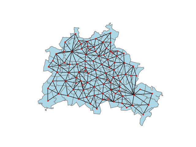
Figure 3: The city of Berlin divided into districts: the Queen adjacency graph

Regarding the benchmark set Real, the instances are specifically designed to support the case study surrounding the real-world application of the $k$-SRD problem as given in Section 4. To generate these graphs, we utilized a collection of GeoJSON files originated from the GitHub repository https://github.com/blackmad/neighborhoods.git. These (168) files encode geographical data structures used to represent geographic features such as points, lines, and polygons. In our context, they represent cities divided into districts, countries divided into regions, or even continents divided into countries, among other possibilities. To generate graphs corresponding to these files, we utilized two Python modules, PySAL and GeoPandas, explicitly developed to work with GeoJSON data. The process of generating graph instances from these files works as follows. First, for each polygon in a file, its centroid point is determined, representing a node of the corresponding graph. Subsequently, the Queen adjacency graph is constructed [13], where two centroids are linked if the two polygons corresponding to these centroids share at least one point on their boundary, meaning their intersection is non-empty.

In Figure 3, one can see an illustration of a graph instance generated for a specific GeoJSON file containing information about the division of the city of Berlin into districts.

3.2 The parameter tuning of the VNS approach

Based on preliminary results, we categorized the instances into three groups: ($i$) small-sized, consisting of instances with $n<30$; ($ii$) middle-sized, comprising instances with $30\leq n<100$; and ($iii$) large-sized, otherwise.

For small-sized instances, a time limit of 300 CPU seconds was set; for middle-sized instances, the time limit was extended to 600 CPU seconds, and for large-sized instances, it was further increased to 1200 CPU seconds, i.e. 20 minutes. It is important to note that the same time limit was applied to all four approaches. In addition, the parameter $num\_iter$ (the iteration limit criterion) of the VNS approach was set to 5000 for all instances.

The rest of parameter values utilized in our VNS across all instances were: $r_{\min}=1$, $r_{\max}=10$, $move\_{prob}=0.5$, $cutoff=100$, and $tries=10$.

3.3 Experimental results

This section reports the experimental results of the four competitors. We consider $k\in\{2,3,4,5\}$ for all our experiments following the same experimental methodology from [24]. The results on benchmark set Random are presented in seven tables, grouped according to different value of $n\in\{10,15,20,30,45,50,100\}$. The results on benchmark set Wireless are reported in four tables, one table per each value of $k$.

3.3.1 Results on benchmark set Random

Experimental results on benchmark set Random for $n\in\{30,50,100\}$ are shown in Tables 1–3. The remaining results are given in B, see Tables 7–10. These tables are organized as follows. The first two columns provide characteristics of respective instance in terms of the graph size ($n$) and its density (that refers to column index), for the details of the generation and how these instances are labeled, we refer to [24]. The third column represents the value of $k$. Next four blocks report the results of Greedy, Vns, Ilp and Benders approach, respectively. For each of two exact approaches and the related blocks, two statistics are shown: the obtained solution quality (column ${obj}$) and the overall running times (column $t[s]$). For Greedy approach, its running times are omitted as these were consistently less than 1 second, thus significantly lower than the other three approaches. For the Vns approach, apart from the reported average solution quality and average running times of achieving best solutions over 10 runs for each instance, additional information is shown – (relative) standard deviation (in percentage) for solution quality over 10 runs (column $\sigma[\%]$). In case of Benders approach, the obtained dual bound (column dual) is additionally provided. The best obtained results among the four competitor approaches are displayed in bold.

The following conclusions may be drawn from the obtained numerical results reported in Tables 1–3.

• For the instances with $n=30$ and small $k\in\{2,3\}$ one could notice that Ilp was able to find a proven optimal solution for all problem instances while its running times increase dramatically when moving from $k=2$ to $k=3$. The Benders approach was running out of the time limit for two cases but delivering dual (lower) bounds which match the value of the corresponding optimal solutions. Concerning our Vns approach, it delivers solutions whose quality is equal to the known optimal solutions. In most cases, its running times are comparable to those of the Ilp approach. Moreover, the initial solutions of Vns obtained by Greedy approach are significantly improved in the search phase of Vns.

• For the instances with $n=30$ and larger $k\in\{4,5\}$, Ilp could not even construct corresponding ILP model within the given memory limit. The Benders approach could not find a proven optimal solution for any of the problem instances. Average solutions quality of Vns approach is significantly better than the quality of solutions provided by the Greedy approach. One can notice that the lower bounds reported by the Benders approach lead to the conclusion that the solutions of VNS are not far from the optimal ones, if not matching the optimal ones.

• For the instances with $n=50$ and $k=2$ one could notice that Ilp could find a proven optimal solution for all 5 problem instances. This was possible for Benders approach on 3 problem instances whereas for two remaining cases it is running out of the given time limit. The average solution quality of Vns approach matches the quality of optimal solutions in 4 (out of 5) problem instances and failing to do it for just one case (29.3 versus 29). In all cases, Vns was able to significantly improve over the initial solutions obtained by Greedy approach.

• For the instances with $n=50$ and $k\in\{3,4,5\}$ one could see that the exact Ilp and Benders approaches could not find a proven optimal solution for any problem instances due to occurred memory issues of initializing ILP model and reaching the given time limit to run the algorithm, respectively. Our Vns approach again has delivered significantly better (average) results than those of Greedy approach.

• For the instances with $n=100$ and $k=2$ we notice that Ilp could find a proven optimal solution for all (5) problem instances whereas Benders approach could find none of them along with delivering relatively weak dual bounds. The (average) quality of solutions obtained by Vns are within $\approx$ 4% gap from the quality of known optimal solutions. Moreover, Vns significantly improves over the initial solutions provided by Greedy approach.

• For the instances with $n=100$ and $k\in\{3,4,5\}$, Ilp cannot find a proven optimal solution due to memory issues. The Benders approach is running out of time and delivering consistently weak dual bounds. Again, the obtained (averaged) solutions of Vns are significantly better than those of Greedy approach – in some case the relative improvements are around 10%.

Instance		$k$	Greedy	VNS			Ilp		Benders
$n$	index		obj	$\overline{obj}$	$\sigma[\%]$	$\overline{t}_{best}[s]$	obj	$t[s]$	obj	dual	$t[s]$
30	1	2	20	17.0	0.00	19.0	17	4.7	17	17	41.2
	2		20	17.0	0.00	1.6	17	6.5	17	17	28.4
	3		21	17.0	2.8	10.6	17	8.3	17	17	87.4
	4		17	16.0	0.0	0.3	16	1.1	16	16	36.0
	5		18	17.0	0.0	4.5	17	6.6	17	17	23.3
30	1	3	23	19.0	0.0	249.4	19	208.9	0	19	TL
	2		23	20.0	0.0	45.1	20	222.2	20	20	373.6
	3		25	20.0	0.0	3.7	20	380.5	0	19	TL
	4		21	19.0	0.0	4.7	19	185.2	19	19	423.9
	5		22	20.0	0.0	29.6	20	218.1	20	20	491.9
30	1	4	26	20.8	2.0	126.1	-	-	0	19	TL
	2		26	21.0	0.0	104.8	-	-	0	20	TL
	3		29	21.0	0.0	374.3	-	-	0	19	TL
	4		24	20.1	1.6	40.7	-	-	0	19	TL
	5		25	21.3	2.2	554.0	-	-	0	20	TL
30	1	5	28	22.4	2.3	346.9	-	-	0	19	TL
	2		29	23.5	4.1	47.6	-	-	0	20	TL
	3		30	23.2	2.7	452.8	-	-	0	19	TL
	4		26	21.6	3.2	202.2	-	-	0	19	TL
	5		27	23.0	2.0	63.6	-	-	0	20	TL

Table 1: Comparison of the approaches on benchmark set Random for $n=30$.

Instance		$k$	Greedy	VNS			Ilp		Benders
$n$	index		obj	$\overline{obj}$	$\sigma[\%]$	$\overline{t}_{best}[s]$	obj	$t[s]$	obj	dual	$t[s]$
50	1	2	31	29.0	0.0	25.5	29	32.9	0	28	TL
	2		31	28.0	0.0	13.1	28	15.2	28	28	439.6
	3		34	28.0	0.0	60.7	28	28.7	28	28	399.8
	4		33	28.0	0.0	15.6	28	21.6	28	28	375.8
	5		36	29.3	0.0	120.6	29	25.2	0	28	TL
50	1	3	36	33.6	1.6	525.6	-	-	0	28	TL
	2		36	33.0	1.5	339.8	-	-	0	28	TL
	3		40	32.4	1.4	246.5	-	-	0	28	TL
	4		38	32.5	2.2	157.4	-	-	0	28	TL
	5		43	34.3	3.0	304.4	-	-	0	29	TL
50	1	4	40	35.6	2.0	312.9	-	-	0	28	TL
	2		40	35.6	2.0	34.1	-	-	0	28	TL
	3		44	36.9	2.4	91.5	-	-	0	28	TL
	4		42	35.1	1.5	18.2	-	-	0	28	TL
	5		47	38.1	2.5	564.7	-	-	0	28	TL
50	1	5	44	40.6	2.9	174.9	-	-	0	28	TL
	2		44	40.0	2.1	92.3	-	-	0	28	TL
	3		48	42.3	2.4	262.7	-	-	0	27	TL
	4		45	40.3	2.5	130.3	-	-	0	28	TL
	5		50	42.9	2.9	406.3	-	-	0	29	TL

Table 2: Comparison of the approaches on benchmark set Random for $n=50$.

Instance		$k$	Greedy	VNS			Ilp		Benders
$n$	index		obj	$\overline{obj}$	$\sigma[\%]$	$\overline{t}_{best}[s]$	obj	$t[s]$	obj	dual	$t[s]$
100	1	2	65	58.3	1.2	420.4	57	402.6	0	49	TL
	2		68	60.4	1.2	586.8	58	752.2	0	49	TL
	3		66	62.1	0.9	499.8	60	775.1	0	52	TL
	4		64	60.4	2.1	445.0	58	296.5	0	50	TL
	5		61	58.9	0.5	188.0	57	315.7	0	50	TL
100	1	3	79	74.5	2.8	696.4	-	-	0	49	TL
	2		82	78.2	2.4	782.6	-	-	0	49	TL
	3		79	76.8	1.3	715.6	-	-	0	51	TL
	4		77	75.9	1.1	511.0	-	-	0	50	TL
	5		72	69.5	1.0	483.2	-	-	0	49	TL
100	1	4	86	77.7	3.0	810.8	-	-	0	49	TL
	2		92	82.8	1.4	831.1	-	-	0	49	TL
	3		89	82.6	1.8	702.7	-	-	0	51	TL
	4		86	79.1	2.2	690.1	-	-	0	50	TL
	5		81	75.8	2.0	684.8	-	-	0	50	TL
100	1	5	92	89.0	2.2	740.8	-	-	0	49	TL
	2		98	90.8	1.7	1035.9	-	-	0	49	TL
	3		95	92.5	1.5	804.8	-	-	0	51	TL
	4		94	91.4	1.6	840.9	-	-	0	49	TL
	5		88	85.5	1.4	815.2	-	-	0	49	TL

Table 3: Comparison of the approaches on benchmark set Random for $n=100$.

3.3.2 Results on benchmark set Wireless

Experimental results on this benchmark set are grouped by different values of $k$ and thus provided in four different tables (one table per each value of $k$). The results for $k=3$ and $k=4$ are displayed in Tables 4 and 5 respectively; the rest of the results can be found in Tables 11–12 of C. The tables are organized similarly as those from the previous section except the columns describing the characteristics of an instance. Namely, the first column provides the size of a graph ($n$) and the second value of radius ($R$) indicates the density of a graph (the larger the radius, the larger the density of a graph is). The best obtained results among the four competitor approaches are displayed in bold.

The following conclusions may be drawn from these results.

• For the instances with $n=20$ and $k=3$, one can see that Ilp and Benders approaches are efficient in solving them all to proven optimality. Our Vns approach could find an optimal solution with a remarkably short running time. The results of Greedy approach seem not to deviate much from the optimal results. Note that the instances with a larger density are easier to be solved.

• For the larger instances with $n\geq 50$ and $k=3$, the exact approaches could not find a proven optimal solution, except for the one problem instance where the Benders approach succeeded. This is due to the encountered issues with reaching the memory or time limit. In seven (out of eight) cases the obtained solutions of Vns are significantly better than that of Greedy approach.

• For the smallest instances with $n=20$ and $k=4$, the exact Ilp approach struggles to solve these instances achieving a success in case of one problem instance ($n=20$ and $R=0.3$). Benders approach demonstrates better performance by solving three (out of four) problem instances. Our Vns finds optimal solutions for all of these problem instances within the time of 1 minute.

• For the larger instances with $n\geq 50$ and $k=4$, the exact Ilp and Benders approaches could not solve any of the problem instances due to exceeding the provided memory and time resources, respectively. Our Vns could find a better solution on six (out of eight) problem instances when compared to the solutions obtained by Greedy approach.

Instance		Greedy	VNS			Ilp		Benders
$n$	$R$	obj	$\overline{obj}$	$\sigma[\%]$	$\overline{t}_{best}[s]$	obj	$t[s]$	obj	dual	$t[s]$
20	0.3	15	14.0	0.0	0.1	14	5.73	14	14	31.1
	0.4	12	12.0	0.0	0.0	12	51.11	12	12	101.0
	0.5	7	6.0	0.0	1.5	6	41.56	6	6	44.6
	0.6	4	4.0	0.0	0.0	4	3.14	4	4	9.8
50	0.3	18	16	0.0	226.4	-	-	0	15	TL
	0.4	14	13.1	0.0	117.4	-	-	0	11	TL
	0.5	10	8.4	0.0	128.7	-	-	0	7	TL
	0.6	7	6	0.0	87.7	-	-	6	6	1402.7
100	0.3	23	21.2	10.1	461.6	-	-	0	13	TL
	0.4	17	14.4	8.3	393.5	-	-	0	10	TL
	0.5	12	12	0.0	0.0	-	-	0	7	TL
	0.6	9	8.2	5.1	222.7	-	-	0	6	TL

Table 4: Comparison of the approaches on benchmark set Wireless for $k=3$.

Instance		Greedy	VNS			Ilp		Benders
$n$	$R$	obj	$\overline{obj}$	$\sigma[\%]$	$\overline{t}_{best}[s]$	obj	$t[s]$	obj	dual	$t[s]$
20	0.3	17	16	0.0	1.4	16	135.2	16	16	144.3
	0.4	14	13	0.0	49.1	19	TL	0	13	TL
	0.5	8	7	0.0	11.6	43	TL	7	7	267.9
	0.6	5	5	0.0	0.0	46	TL	5	5	33.1
50	0.3	21	21	2.8	0.0	-	-	0	15	TL
	0.4	16	15.6	0.0	18.7	-	-	0	12	TL
	0.5	12	11.1	0.0	157.1	-	-	0	8	TL
	0.6	8	7	0.0	16.9	-	-	0	7	TL
100	0.3	28	27.4	0.0	261.5	-	-	0	14	TL
	0.4	21	20	3.3	415.6	-	-	0	10	TL
	0.5	15	15	5.1	0.0	-	-	0	8	TL
	0.6	11	10.6	0.0	225.0	-	-	0	7	TL

Table 5: Comparison of the approaches on benchmark set Wireless for $k=4$.

3.3.3 Summary results on benchmark set Real

In order to show the efficiency of our Vns approach on benchmark set Real, the following methodology is applied. We take into a consideration those instances for which the both exact approaches were successful in solving them. Then, the obtained solutions of Greedy and Vns approaches are compared with the exact solutions in terms of average solution qualities grouped by $k\in\{2,3,4,5\}$ (one row per each value $k$). This is reported results in Table 6. Note that due to a high number of instances, Vns is executed only once per each instance. However, due to a relatively small (relative) standard deviation obtained for the solutions of Vns on both benchmark sets, Random and Wireless, it is not expected that overall conclusions obtained for one-run Vns execution scenario will deviate significantly from the ten-runs Vns experimental scenario.

$k$	Greedy	Vns	Ilp/Benders	#instances
2	20.98	20.15	20.11	66
3	15.58	14.74	14.74	43
4	13.96	13.00	13.00	25
5	12.47	11.58	11.58	17

Table 6: Comparison between the four approaches on benchmark set Real: the case of the instances solved by Ilp and Benders.

The following conclusions may be drawn from there.

• The number of instances optimally solved is quickly deteriorating as $k$ increases.

• Vns is able to find optimal solutions for all cases where Ilp/Benders were able to solve an instance (with an exception of a few instances for the case $k=2$).

• Greedy approach is significantly outperformed by the Vns approach.

• We stress out that our two heuristic approaches are able to produce approximate solutions of reasonable quality (both are significantly better from the trivial solution) on the rest of the instances where the exact approaches could deliver none or only solutions of poor quality.

3.4 Comparison between the two heuristic approaches

To compare the two of our heuristic approaches, the Greedy and Vns, we have additionally provided Figure 4(a)–4(b) for benchmark set Random and Figure 5(a)–5(b) for benchmark set Wireless. These plots display the average relative improvements of Vns over Greedy in terms of solution quality. The instances are grouped by $n$ and by $k$ (the values shown on $x$-axis) separately; thus, two plots are generated per each benchmark set. Additionally Figure 6 displays the average relative improvements of Vns over Greedy in terms of solution quality for all instances from benchmark set Real where the instances are grouped by $k$.

(a) Instances grouped by $n$

(b) Instances grouped by $k$.

Figure 4: Relative average improvements of Vns over Greedy approach on benchmark set Random.

(a) Instances grouped by $n$

(b) Instances grouped by $k$.

Figure 5: Relative average improvements of Vns over Greedy approach on benchmark set Wireless.

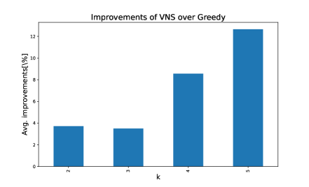
Figure 6: Relative average improvements of Vns over Greedy approach on benchmark set Real.

The following conclusions may be drawn from generated plots.

• For the instances from the benchmark set Random grouped by graph dimension ($n$), average improvements of the quality of initial solutions of Vns range from respectable 12-16% for $10\leq n\leq 50$ whereas for the largest group of instances with $n=100$ this percentage still remains significant, and is at about 5%.

• For the instances from benchmark set Random grouped by $k$ values, average relative improvements of Vns range from 8.5% for $k=2$ to 13% for the group with $k=4$.

• For the instances from the benchmark set Wireless grouped by $n$, the average improvements of Vns range from about 6% for the largest $n=100$ and $\approx$7.7% for smaller $n\in\{20,50\}$.

• For the instances from the benchmark set Wireless grouped by $k$, the average improvements expectedly deteriorate with the increase of $k$ value. For the smallest $k=2$ the average improvements are about an excellent 15% and decrease for the largest case $k=5$ to 3%. This is mainly due to a high number of generated attacks that have to be verified for the existence of a defense strategy which significantly reduces the overall number of performed iterations of the Vns approach.

• For the instances from the benchmark set Real, average relative improvements of Vns range from 3.5%–3.8% for $k\in\{2,3\}$ to more than 12% for the largest case $k=5$.

3.5 Statistical analysis

To verify the statistical significance of the observed differences between the four approaches, we performed the following statistical methodology. First, Friedman’s test was executed for all four competitor approaches on all problem instances of the Random and Wireless benchmark sets separately. After that, in cases when the null hypothesis was rejected ($H_{0}$ says that competitor approaches are statistically equally good) pairwise comparisons were further performed by using the Nemenyi post-hoc test [30].

The outcome is represented within critical difference (CD) plots. A CD plot positions each approach on the horizontal axis according to its average ranking. Then, the CD is computed for a significance level of 0.05. If the difference is small enough, that is, no statistical difference is detected, a horizontal bar connecting statistically equal approaches is drawn. In case no result has been returned by an algorithm, we simply assign a large value (e.g. 1000) providing with the largest possible ranking.

(a) Benchmark set Random

(b) Benchmark set Wireless

(c) Benchmark set Real

Figure 7: CD plots showing statistical differences between the four approaches on the results summarized over all $k\in\{2,3,4,5\}$.

The following conclusions may be drawn from the statistical analysis conducted, as depicted in Figures 7(a)– 7(c).

• For the benchmark set Random, Vns approach achieves the best average ranking while the other three approaches are far behind, obtaining the average ranking that is close to the value of three. Additionally, Vns is performing statistically significantly better from the remainder of the competitors and between three of them no statistically significant difference occurred.

• For the benchmark set Wireless, Vns again gains the best average ranking, which is for the whole ranking of one better than the second best Greedy approach. The worst average ranking is delivered by Benders and Ilp, in this order. Again, the best performing approach is Vns, which significantly outperforms the Greedy approach in terms of obtained solution quality. Statistically the worst performing approaches are Benders and ILP as they could not usually deliver any solution for larger $k$ values.

• For the benchmark set Real, Vns again obtains the best average ranking. The second best average ranking is achieved by Greedy approach, primarily due to its consistent delivery of feasible solutions, unlike the two exact competitor algorithms. Note that again the solutions of Vns are statistically significantly better than that of the Greedy approach.

4 Application of the $k$-SRD problem to a real-world scenario

In the pursuit for applicability, we decided to visualize and interpret the results of Vns approach on a few real-world instances generated from GeoJSON files, see Section 3. For a real-world case scenario we opt for a location problem which concern placing fire stations with a number of fire trucks in a city at appropriate locations under specific constraints. As follows we list some numbers, mainly taken from Wikipedia, as the reference point for this real-world problem; e.g. the number of fire stations in the city of Dublin is 14, in the city of Berlin is 35, in Chicago there are 98 fire stations, while in the city of New York, 254 stations are installed. The number of available fire trucks in Chicago is 61, and in the city of New York is 143. In the city of Berlin, in 2019, its Fire Defense received 478,281 emergency calls, known as the busiest of all fire services in Germany. Approximately 83% of the alarms per year are for the emergency services, 5% for technical assistance and only about 2% for firefighting. If we assume that 4 hrs are needed on average for a complete (successful) intervention (from exit of the fire engine from the station to its re-entry after the intervention and its re-use), the number of real fire emergencies that may simultaneously occur in this city is expected to be $\approx k=5$.

Let us find the best decisions of installing fire stations at certain districts under the following (simplified) constraints.

• At most one fire station might be built per each district.

• At any chosen location for building a fire stations, one or more fire trucks can be placed.

• One fire truck placed at a fire station of a district can serve to extinguish fire occuring in that district or the neighboring districts. This reflects on realistic scenario of demanding quick speed of reaction in this kind of emergency. For example, sending a fire truck from the westernmost part of the city to serve in a district diametrically opposite will consume valuable time, particularly in big cities with large diameters and expected heavy traffic congestion.

• At least one truck is always kept to secure that district, i.e. all but one fire truck at any station are available to be sent to neighboring districts for interventions.

The given value of $k$ represents an estimator for the number of districts that can be simultaneously under fire. We additionally assume a simplified scenario that one fire truck is sufficient for extinguishing any fire (may not be that realistic in a huge threat). The aim is to find locations to build fire stations along with the number of fire trucks in each of them so that any fire scenario that occurs in $k$ different districts simultaneously, can be treated safely.

We demonstrate visually applications of the above problem on a few world cities whose graph representations are extracted from corresponding GeoJSON files, see Section 3. Three cities are chosen: Szczecin and Cincinnati as the representatives for medium-sized instances and Pittsburgh as a representative of large-sized instance. The value of $k$ is chosen from the set $\{5,6,8\}$. The city of Szczecin comprises 36 districts into one connected graph. The city of Cincinnaty consists of 45 districts, also forming a connected graph. On the other hand, the city of Pittsburgh consists of 90 districts subdivided into 4 disjoint regions. Note that none of the exact approaches could successfully solve any of these instances, and the solutions provided by VNS consistently exhibit higher quality than those of the Greedy approach.

The solutions produced by Vns for all three cities (and all three values of $k$) are displayed in Figures 8(a)–10(c). The following conclusions are made for the city of Szczecin.

• For $k=5$ the solution is equal to 26. 10 districts are chosen as hubs for building fire stations where at least one fire truck is placed. There are two centralized hubs that each keep five fire trucks and one that keeps three trucks. There are six fire stations with two trucks and one with one truck. For the two hubs with dominant number of trucks, one is located in the geographically largest district, and the second is among the smallest districts, close to the city center whose reachability is high.

• For $k=6$, the solution is equal to 28. Nine fire stations are supposed to be built. One station keeps seven trucks, one with six trucks and one with five trucks. The others keep two or less than two trucks.

• For $k=8$, the obtained solution is equal to 33. Eight fire stations are suggested to be built. Again, three major stations are distinguishable in terms of the number of trucks. Two of them keep nine trucks, and one comes with six trucks. The others keep two or less than two trucks.

• Interestingly, two locations for fire stations with a large number of trucks match for any $k\in\{5,6,8\}$. For $k\in\{6,8\}$, three of the locations match. This can be argued by the fact that the corresponding nodes have the highest centrality degree among most other nodes, indicating their high immediate reachability. Thus, they can cover many surrounding districts if enough trucks are placed. The two common nodes for each value of $k$ have degree centrality score of 0.25 and 0.31, and are among the highest for all nodes.

The following conclusions are drawn for the graph of the city of Cincinnati.

• For $k=5$, the obtained solution is equal to 36. 19 fire stations are suggested to open. There is no station that keeps more than four fire trucks. There is just one station keeping 4 trucks and many (5) of them with three. The stations with more fire trucks seem to be geographically uniformly distributed.

• For $k=6$, the obtained solution is equal to 41. 15 fire stations are suggested to be built. There are two stations with six fire trucks and four stations with four fire trucks while the remaining stations comprise two or less fire trucks.

• For $k=8$, the obtained solution is equal to 45. 16 fire stations are suggested to be built. Two fire stations keep seven fire trucks, two stations with five, and three with four fire trucks, while for nine stations just one truck is assigned (mainly located at the boundary of the whole city region). The seven stations that dominate in term of number of kept trucks seem to be geographically equally distributed over the city region.

• The two nodes assigned with the largest number of trucks (7) have the associated highest centrality degree scores (0.18 and 0.16) in the graph.

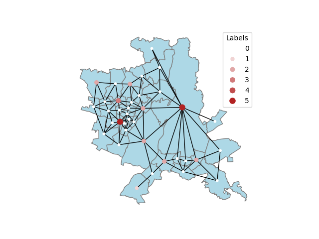
(a) $k=5$

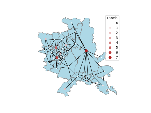
(b) $k=6$

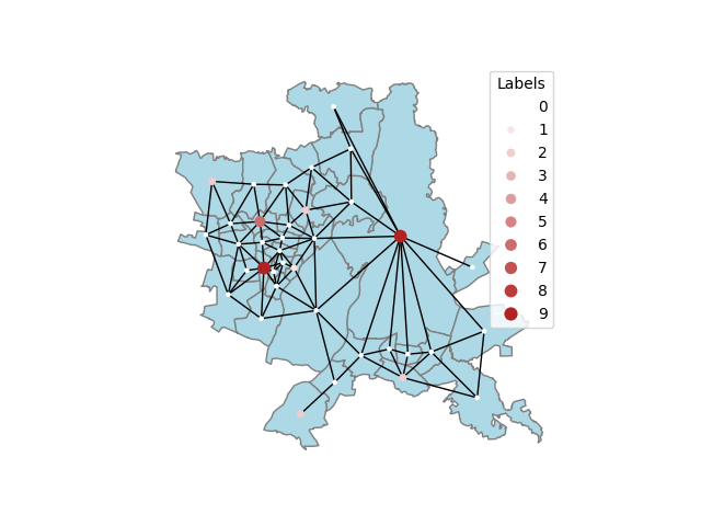
(c) $k=8$

Figure 8: Graph of the city of Szczecin.

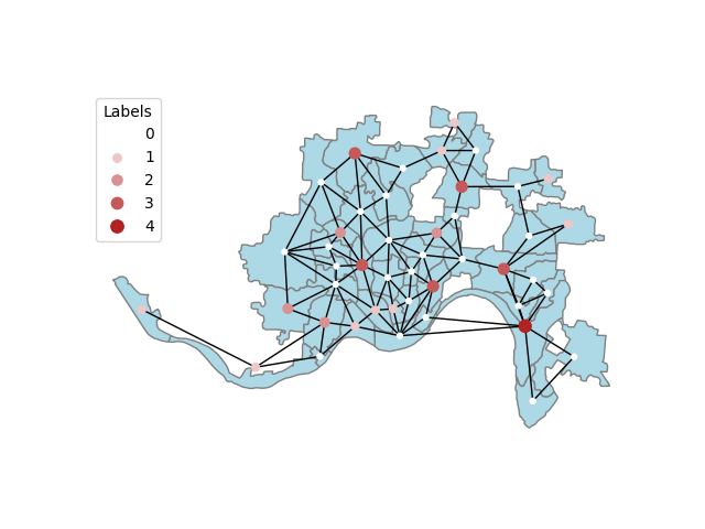
(a) $k=5$

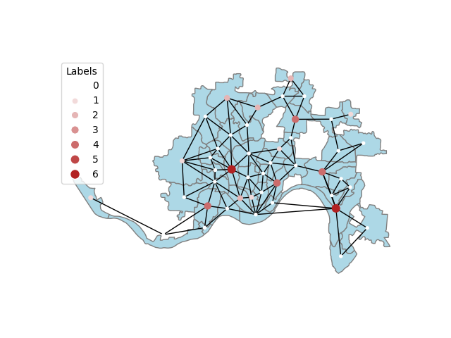
(b) $k=6$

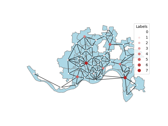
(c) $k=8$

Figure 9: Graph of the city of Cincinnati.

Last but not least, we visualize and analyze the solution of Vns for the city of Pittsburgh. The following facts are observed.

• For $k=5$, the obtained solution is equal to 67. There are 30 locations suggested for a hub, i.e. to build a fire station. There is one station keeping five fire trucks, and three with four fire trucks. Three stations also hold three fire trucks, and the rest of them store two or less trucks.

• For $k=6$, the obtained solution is equal to 73. There are 32 locations chosen for building fire stations. Four of them come with five fire trucks, one with four and seven of them with three trucks.

• For $k=8$ the obtained solution is equal to 81. There are 31 locations suggested for building a fire station. Three of them keep six fire trucks, five of them keep five trucks, and four of them three trucks.

• While for $k=6$ and $k=8$, the locations of stations with the highest number of trucks mostly match, for the case $k=5$ it is less clear; however, there exist two locations which correspond to the locations with a larger number of trucks in case of both $k=6$ and $k=8$.

• Concerning the mentioned two common dominant locations (nodes) in terms of number of trucks located for each $k\in\{5,6,8\}$, their centrality degrees are among the highest in the graph and are equal to 0.09 and 0.06.

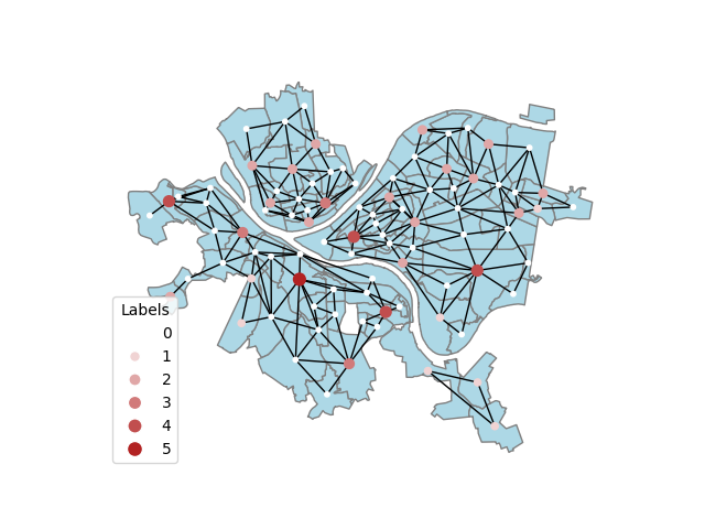
(a) $k=5$

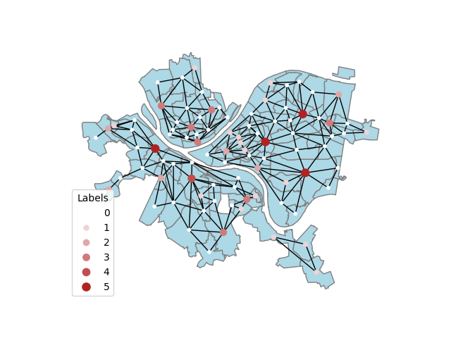
(b) $k=6$

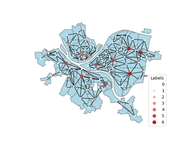
(c) $k=8$

Figure 10: Graph of the city of Pittsburgh.

5 Conclusions and future work

In this paper we have dealt with solving the $k$-strong Roman domination ($k$-SRD) problem with arbitrary $k\geq 2,k\in\mathbb{N}$. The $k$-SRD problem is extremely hard to solve, since even verifying the feasibility of a solution is exponential with the number of nodes in graph. We have proposed two heuristic approaches: ($i$) a greedy approach based on node coverage information, and ($ii$) an improved variable neighborhood search (VNS) algorithm that uses the greedy solution as the initial solution. Our VNS approach is based on three basic principles. First, a shaking procedure that shakes components of the best solution based on roulette selection by always generating a one better but possibly infeasible solution. Second, relaxed feasibility is checked during the search; this concept is called quasi-feasibility. Here, a set of $k$-attacks in the vicinity of the nodes of the considered solution is carefully generated. Then, for all these attacks, a strategy is probed for defending them. Two strategies are used for defense – one deterministic and one probabilistic (roulette-based). The fitness score of the solution is made up of two components: the number of predefined attacks that cannot be defended and the sum of all labels of the given solution. The third core principle of VNS is an efficient local search procedure based on the 2-decomposition operator on a swap basis, which includes an initial improvement strategy and an internal caching mechanism to ensure efficient execution.

Two of our heuristic approaches are compared with the two existing exact approaches from the literature, integer linear programming (ILP) and Benders-based approaches. This comparison is performed on randomly generated graphs from the literature as well as on two newly introduced benchmark sets: wireless ad hoc networks with different densities and real-word instances generated from corresponding GeoJSON files. These files represent spatial data of cities divided into districts, countries into regions, etc. While the two exact approaches could only handle small to medium sized instances and some slightly larger ones with $k=2$, they were not able to handle the largest instances as they consistently encountered issues with memory (ILP) or time (the Benders-based approach). Our VNS approach was able to consistently and significantly improve the results of the greedy approach on instances of different sizes and distributions. Moreover, for most instances solved by some of the exact approaches, our VNS approach was able to achieve these solutions or produce near-optimal, statistically equally good solutions in reasonable time. For the real-world instances and their solutions obtained from solving the $k$-SRD problem by the VNS approach for larger, and never so-far tested values of $k\in\{6,8\}$, a case study of deciding on opening locations for fire stations in the neighbourhoods and assigning a number of fire trucks to each of these locations to be able to handle at most $k$ simultaneous fires is discussed.

For future work, one could design an approach for much larger problem instances with thousands of nodes. Note that our VNS approach might be limited to an application of graphs with up to a few hundred nodes; the number of predefined attacks grows rapidly with the size of the graph, making the approach computationally expensive per iteration. One idea is to transform the current VNS into a more scalable VNS by intelligently clustering a graph into some dependent groups of nodes, e.g. using community detection algorithms. Then, the standalone VNS would be applied to each of the obtained components (one could also develop a parallel implementation). The combination of the obtained solutions for each of the subgraphs induced by the clusters into a high quality solution of the initial graph could be done by a local search based procedure for detected critical nodes. Another aspect could be to design a different meta-heuristic approach that builds on our greedy approach by randomizing it and improving the generated solution e.g. by the established appropriate local search procedure.

Acknowledgments. Marko Djukanovic, Stefan Kapunac, and Dragan Matic acknowledge are partially funded by the project entitled ”Developing models and algorithms of Artificial intelligence for solving computationally hard combinatorial optimization problems” under no. 1259086 supported by the Ministry of Scientific and Technological Development and Higher Education of Republic of Srpska. Marko Djukanovic is additionally supported by the project grant ”Theoretical and computational aspects of solving Roman domination problems” funded by the Ministry of Civil Affairs of Bosnia and Herzegovina under no. 1259074.

Appendix A Pseudocodes supporting is_attack_defended() function

1:Input: solution $s$, graph $G=(V,E),k,all\_alternatives,reduced\_attack,defending\_nodes$

2:Output: a pair attack_defended, defending_nodes

3:for $alternative\in all\_alternatives$ do

4:    $attack\_defended\leftarrow True$

5:    for $v\in reduced\_attack$ do

6:        $u\leftarrow alternative[v]$

7:        if $u$ can help $v$ then

8:           add $u$ to $defending\_nodes$

9:        else

10:           $attack\_defended\leftarrow False$

11:           break

12:        end if

13:    end for

14:    if $attack\_defended$ then

15:        return $attack\_defended,defending\_nodes$

16:    end if

17:end for

18:return $False,\emptyset$

Algorithm 6 Function deterministic_defense()

1:Input: solution $s$, graph $G=(V,E),k,reduced\_attack,defending\_nodes,tries>0$

2:Output: a pair attack_defended, defending_nodes

3:while $tries>0$ do

4:    $attack\_defended\leftarrow True$

5:    $tries\leftarrow tries-1$

6:    for $v\in reduced\_attack$ do

7:        $candidates\leftarrow[]$

8:        for $u\in N(v)$ do

9:           $diff\leftarrow$ number of available FAs in node $u$

10:           $candidates.add([\underbrace{u,\ldots,u}_{\emph{diff}\textrm{ times}}])$

11:        end for

12:        if $candidates.size()=0$ then

13:           $attack\_defended\leftarrow False$

14:           break

15:        end if

16:        $selected\_u\leftarrow$ random element from $candidates$

17:        add $selected\_u$ to $defending\_nodes$

18:    end for

19:    if $attack\_defended$ then

20:        return $attack\_defended,defending\_nodes$

21:    end if

22:end while

23:return $False,\emptyset$

Algorithm 7 Function roulette_defense()

Appendix B Complete results for benchmark set Random

Table 7: Comparison of the approaches on benchmark set Random for $n=10$.

Instance		$k$	Greedy	VNS			Ilp		Benders
$n$	index		obj	$\overline{obj}$	$\sigma[\%]$	$\overline{t}_{best}[s]$	obj	$t[s]$	obj	dual	$t[s]$
10	1	2	7	6	0.0	0.0	6	0.1	6	6	0.7
	2		6	6	0.0	0.0	6	0.1	6	6	0.7
	3		6	6	0.0	0.0	6	0.1	6	6	2.5
	4		6	5	0.0	0.0	5	0.0	5	5	1.2
	5		6	6	0.0	0.0	6	0.1	6	6	1.8
10	1	3	8	7	0.0	0.0	7	0.5	7	7	2.4
	2		7	6	0.0	0.0	6	0.4	6	6	3.8
	3		7	7	0.0	0.0	7	0.4	7	7	3.0
	4		8	6	0.0	0.1	6	0.3	6	6	2.9
	5		7	7	0.0	0.0	7	0.4	7	7	2.9
10	1	4	9	7	0.0	0.4	7	1.6	7	7	3.4
	2		8	7	0.0	0.0	7	1.6	7	7	3.4
	3		8	7	0.0	0.5	7	1.4	7	7	4.1
	4		9	7	0.0	0.4	7	1.3	7	7	4.2
	5		8	7	0.0	0.1	7	1.4	7	7	4.4
10	1	5	10	8	0.0	0.1	8	4.1	8	8	6.3
	2		9	8	0.0	0.0	8	2.8	8	8	4.4
	3		9	8	0.0	0.0	8	3.2	8	8	11.5
	4		10	8	0.0	0.0	8	2.7	8	8	7.1
	5		9	8	0.0	0.2	8	2.0	8	8	9.7

Table 8: Comparison of the approaches on benchmark set Random for $n=15$.

Instance		$k$	Greedy	VNS			Ilp		Benders
$n$	index		obj	$\overline{obj}$	$\sigma[\%]$	$\overline{t}_{best}[s]$	obj	$t[s]$	obj	dual	$t[s]$
15	1	2	10	9	0.0	0.0	9	0.9	9	9	5.3
	2		8	8	0.0	0.0	8	0.2	8	8	2.2
	3		9	8	0.0	0.0	8	0.2	8	8	2.8
	4		10	9	0.0	0.0	9	1.2	9	9	5.0
	5		10	9	0.0	0.2	9	0.3	9	9	3.8
15	1	3	12	10	0.0	0.3	10	12.2	10	10	20.2
	2		10	10	0.0	0.0	10	3.6	10	10	12.9
	3		10	9	0.0	0.0	9	1.5	9	9	7.7
	4		12	10	0.0	0.0	10	12.1	10	10	21.3
	5		12	10	0.0	0.0	10	7.1	10	10	22.0
15	1	4	13	11	0.0	0.3	11	51.7	11	11	55.4
	2		12	11	0.0	1.2	11	37.7	11	11	35.4
	3		11	10	0.0	1.1	10	19.0	10	10	36.6
	4		13	11	0.0	1.6	11	104.8	11	11	77.7
	5		14	11	0.0	1.6	11	80.2	11	11	107.0
15	1	5	14	11	0.0	8.8	14	TL	11	11	129.1
	2		13	11	0.0	9.1	11	239.4	11	11	60.0
	3		12	11	0.0	0.7	11	162.9	11	11	72.2
	4		14	12	0.0	2.4	12	TL	0	11	TL
	5		15	12	0.0	5.7	12	TL	12	12	210.0

Table 9: Comparison of the approaches on benchmark set Random for $n=20$.

Instance		$k$	Greedy	VNS			Ilp		Benders
$n$	index		obj	$\overline{obj}$	$\sigma[\%]$	$\overline{t}_{best}[s]$	obj	$t[s]$	obj	dual	$t[s]$
20	1	2	12	11	0.0	0.0	11	1.5	11	11	5.5
	2		13	12	0.0	0.3	12	0.5	12	12	14.0
	3		12	11	0.0	0.0	11	0.9	11	11	6.3
	4		11	11	0.0	0.0	11	0.4	11	11	5.8
	5		12	12	0.0	0.0	12	1.4	12	12	9.3
20	1	3	14	12	0.0	4.9	12	7.7	12	12	24.9
	2		16	13	0.0	1.0	13	17.0	13	13	109.8
	3		14	13	0.0	0.1	13	46.2	13	13	66.2
	4		14	13	0.0	0.4	13	14.7	13	13	38.0
	5		15	13	0.0	1.5	13	41.1	13	13	62.4
20	1	4	16	14	0.0	4.7	14	TL	14	14	224.2
	2		18	14	0.0	17.2	18	TL	0	14	TL
	3		15	13	0.0	103.5	23	TL	13	13	89.5
	4		16	14	0.0	12.6	18	TL	14	14	111.2
	5		17	14	0.0	105.6	22	TL	0	14	TL
20	1	5	18	15	0.0	7.4	-	-	0	14	TL
	2		19	15	2.1	91.1	-	-	0	14	TL
	3		16	14	0.0	43.7	-	-	0	14	TL
	4		17	14	0.0	74.7	-	-	14	14	276.2
	5		19	15	0.0	66.8	-	-	0	14	TL

Table 10: Comparison of the approaches on benchmark set Random for $n=45$.

Instance		$k$	Greedy	VNS			Ilp		Benders
$n$	index		obj	$\overline{obj}$	$\sigma[\%]$	$\overline{t}_{best}[s]$	obj	$t[s]$	obj	dual	$t[s]$
45	1	2	28	26.5	2.0	98.4	26	14.5	26	26	240.3
	2		28	26	0.0	9.1	26	19.5	26	26	311.3
	3		28	26	0.0	7.6	26	35.4	26	26	326.0
	4		28	27	0.0	8.5	27	21.0	0	27	TL
	5		27	26	0.0	27.6	26	10.3	26	26	225.9
45	1	3	35	30	1.6	166.9	-	-	0	27	TL
	2		34	29.3	1.6	283.4	-	-	0	26	TL
	3		35	29.8	2.1	243.7	-	-	0	27	TL
	4		35	29.8	2.1	226.9	-	-	0	27	TL
	5		34	29.4	1.8	276.4	-	-	0	26	TL
45	1	4	40	32.9	3.0	191.5	-	-	0	28	TL
	2		39	32.1	1.8	259.6	-	-	0	25	TL
	3		40	33.5	2.5	228.6	-	-	0	26	TL
	4		40	32.9	3.0	276.1	-	-	0	26	TL
	5		38	32.3	2.5	208.7	-	-	0	27	TL
	1		43	36.4	1.4	333.4	-	-	0	28	TL
45	2	5	42	36.0	1.3	363.0	-	-	0	26	TL
	3		43	37.9	2.0	244.6	-	-	0	26	TL
	4		43	37.1	2.4	278.8	-	-	0	26	TL
	5		42	35.9	2.4	348.6	-	-	0	26	TL

Appendix C Complete results for benchmark set Wireless

Instance		Greedy	VNS			Ilp		Benders
$n$	$R$	obj	$\overline{obj}$	$\sigma[\%]$	$\overline{t}_{best}[s]$	obj	$t[s]$	obj	dual	$t[s]$
20	0.3	13	12	0.0	0.8	12	0.25	12	12	6.5
	0.4	10	9	0.0	0.2	9	1.16	9	9	7.8
	0.5	6	5	0.0	0.1	5	1.14	5	5	6.6
	0.6	3	3	0.0	0.0	3	0.21	3	3	2.6
50	0.3	15	13	0.0	3.8	-	-	13	13	196.2
	0.4	11	10	0.0	7.7	-	-	10	10	177.6
	0.5	8	6	0.0	4.0	-	-	6	6	64.0
	0.6	6	5	0.0	2.1	-	-	5	5	100.1
100	0.3	18	13	3.0	239.4	-	-	0	13	TL
	0.4	13	10	0.0	24.2	-	-	0	10	TL
	0.5	9	9	0.0	0.0	-	-	0	7	TL
	0.6	7	6	0.0	21.5	-	-	-	-	-

Table 11: Comparison of the approaches on benchmark set Wireless for $k=2$.

Instance		Greedy	VNS			Ilp		Benders
$n$	$R$	obj	$\overline{obj}$	$\sigma[\%]$	$\overline{t}_{best}[s]$	obj	$t[s]$	obj	dual	$t[s]$
20	0.3	19	17	0.0	45.4	-	-	0	16	TL
	0.4	16	14.3	3.4	85.6	-	-	0	14	TL
	0.5	9	8	0.0	10.3	-	-	0	8	TL
	0.6	6	6	0.0	0.0	-	-	6	6	187.0
50	0.3	24	24	0.0	0.0	-	-	0	16	TL
	0.4	18	17.9	0.0	18.9	-	-	0	12	TL
	0.5	14	13.7	3.4	46.9	-	-	0	9	TL
	0.6	9	7	0.0	136.8	-	-	0	7	TL
100	0.3	33	33	0.0	0.0	-	-	-	-	-
	0.4	25	24.6	1.8	182.5	-	-	-	-	-
	0.5	18	18	3.5	0.0	-	-	-	-	-
	0.6	12	12	0.0	0.0	-	-	-	-	-

Table 12: Comparison of the approaches on benchmark set Wireless for $k=5$.

References

- [1] S. Abdullah, E. K. Burke, and B. McColloum. An investigation of variable neighborhood search for university course timetabling. In The 2th Multidisciplinary Conference on Scheduling: Theory and Applications, NY, USA, pages 413–427, 2005.
- [2] M. Álvarez-Ruiz, T. Mediavilla-Gradolph, S. M. Sheikholeslami, J. Valenzuela-Tripodoro, and I. G. Yero. On the strong Roman domination number of graphs. Discrete Applied Mathematics, 231:44–59, 2017.
- [3] B. Balasundaram and S. Butenko. Graph domination, coloring and cliques in telecommunications. Handbook of optimization in telecommunications, pages 865–890, 2006.
- [4] A. Burger, A. De Villiers, and J. Van Vuuren. A binary programming approach towards achieving effective graph protection. In Proceedings of the 2013 ORSSA annual conference, ORSSA, pages 19–30, 2013.
- [5] G. J. Chang. Algorithmic aspects of domination in graphs. Handbook of Combinatorial Optimization: Volume1–3, pages 1811–1877, 1998.
- [6] A. Charpentier, D. Mignon, S. Barbe, J. Cortes, T. Schiex, T. Simonson, and D. Allouche. Variable neighborhood search with cost function networks to solve large computational protein design problems. Journal of Chemical Information and Modeling, 59(1):127–136, 2018.
- [7] M. Chellali, N. Jafari Rad, S. M. Sheikholeslami, and L. Volkmann. Roman domination in graphs. Topics in domination in graphs, pages 365–409, 2020.
- [8] B. N. Clark, C. J. Colbourn, and D. S. Johnson. Unit disk graphs. Discrete mathematics, 86(1-3):165–177, 1990.
- [9] E. Cockayne. Domination of undirected graphs—a survey. In Theory and Applications of Graphs: Proceedings, Michigan May 11–15, 1976, pages 141–147. Springer, 1978.
- [10] E. J. Cockayne, P. A. Dreyer Jr, S. M. Hedetniemi, and S. T. Hedetniemi. Roman domination in graphs. Discrete mathematics, 278(1-3):11–22, 2004.
- [11] W. Goddard and M. A. Henning. Independent domination in graphs: A survey and recent results. Discrete Mathematics, 313(7):839–854, 2013.
- [12] M. Grbić, A. Kartelj, S. Janković, D. Matić, and V. Filipović. Variable neighborhood search for partitioning sparse biological networks into the maximum edge-weighted k-plexes. IEEE/ACM Transactions on Computational Biology and Bioinformatics, 17(5):1822–1831, 2020.
- [13] D. A. Griffith and U. Luhanga. Approximating the inertia of the adjacency matrix of a connected planar graph that is the dual of a geographic surface partitioning. Geographical Analysis, 43(4):383–402, 2011.
- [14] P. Gupta. Domination in graph with application. Indian J. Res, 2(3):115–117, 2013.
- [15] P. Hansen, N. Mladenović, and D. Perez-Britos. Variable neighborhood decomposition search. Journal of Heuristics, 7(4):335–350, 2001.
- [16] P. Hansen, C. Oğuz, and N. Mladenović. Variable neighborhood search for minimum cost berth allocation. European Journal of Operational Research, 191(3):636–649, 2008.
- [17] V. C. Hemmelmayr, K. F. Doerner, and R. F. Hartl. A variable neighborhood search heuristic for periodic routing problems. European Journal of Operational Research, 195(3):791–802, 2009.
- [18] M. A. Henning. A survey of selected recent results on total domination in graphs. Discrete Mathematics, 309(1):32–63, 2009.
- [19] M. A. Henning and S. T. Hedetniemi. Defending the Roman Empire—A new strategy. Discrete Mathematics, 266(1-3):239–251, 2003.
- [20] M. Ivanović and D. Urošević. Variable neighborhood search approach for solving Roman and weak Roman domination problems on graphs. Computing & Informatics, 38(1), 2019.
- [21] B. Jarboui, H. Derbel, S. Hanafi, and N. Mladenović. Variable neighborhood search for location routing. Computers & Operations Research, 40(1):47–57, 2013.
- [22] S. Kapunac, A. Kartelj, and M. Djukanović. Variable neighborhood search for weighted total domination problem and its application in social network information spreading. Applied Soft Computing, 143:110387, 2023.
- [23] A. Khandelwal, K. Srivastava, and G. Saran. On Roman domination of graphs using a genetic algorithm. In Computational Methods and Data Engineering: Proceedings of ICMDE 2020, Volume 1, pages 133–147. Springer, 2020.
- [24] Z. Liu, X. Li, and A. Khojandi. On the -strong Roman domination problem. Discrete Applied Mathematics, 285:227–241, 2020.
- [25] G. Lu, M.-T. Zhou, Y. Tang, Z.-Q. Wu, G.-Y. Qiu, and L. Yuan. A survey on exact algorithms for dominating set related problems in arbitrary graphs. Chinese Journal of Computers, 33(6):1073–1087, 2010.
- [26] N. Mladenović, M. Dražić, V. Kovačevic-Vujčić, and M. Čangalović. General variable neighborhood search for the continuous optimization. European Journal of Operational Research, 191(3):753–770, 2008.
- [27] N. Mladenović and P. Hansen. Variable neighborhood search. Computers & operations research, 24(11):1097–1100, 1997.
- [28] B. Nikolić, M. Djukanović, M. Grbić, and D. Matić. Theoretical studies of the -strong Roman domination problem. arXiv preprint arXiv:2312.14527, 2023.
- [29] A. Pagourtzis, P. Penna, K. Schlude, K. Steinhöfel, D. S. Taylor, and P. Widmayer. Server placements, Roman domination and other dominating set variants. In Foundations of Information Technology in the Era of Network and Mobile Computing: IFIP 17th World Computer Congress—TC1 Stream/2nd IFIP International Conference on Theoretical Computer Science (TCS 2002) August 25–30, 2002, Montréal, Québec, Canada, pages 280–291. Springer, 2002.
- [30] T. Pohlert. The pairwise multiple comparison of mean ranks package (PMCMR). R package, 27(2019):9, 2014.
- [31] A. Poureidi and J. Fathali. Algorithmic results in Roman dominating functions on graphs. Information Processing Letters, 182:106363, 2023.
- [32] Y. Rao, R. Chen, P. Wu, H. Jiang, and S. Kosari. A survey on domination in vague graphs with application in transferring cancer patients between countries. Mathematics, 9(11):1258, 2021.
- [33] V. Roshanaei, B. Naderi, F. Jolai, and M. Khalili. A variable neighborhood search for job shop scheduling with set-up times to minimize makespan. Future Generation Computer Systems, 25(6):654–661, 2009.
- [34] N. Smiti, M. M. Dhiaf, B. Jarboui, and S. Hanafi. Skewed general variable neighborhood search for the cumulative capacitated vehicle routing problem. International Transactions in Operational Research, 27(1):651–664, 2020.