Understanding the Multi-wavelength Thermal Dust Polarization from the Orion Molecular Cloud in Light of the Radiative Torque Paradigm

Dust grains are important in various astrophysical processes and serve as indicators of interstellar medium structures, density, and mass. Understanding their physical properties and chemical composition is crucial in astrophysics. Dust polarization is a valuable tool for studying these properties. The Radiative Torque (RAT) paradigm, which includes Radiative Torque Alignment (RAT-A) and Radiative Torque Disruption (RAT-D), is essential to interpret the dust polarization data and constrain the fundamental properties of dust grains. However, it has been used primarily to interpret observations at a single wavelength. In this study, we analyze the thermal dust polarization spectrum obtained from observations with SOFIA/HAWC+ and JCMT/POL-2 in the Orion Molecular Cloud 1 (OMC-1) region and compare the observational data with our numerical results using the RAT paradigm. We find that the dense gas exhibits a positive spectral slope, whereas the warm regions show a negative one. We demonstrate that a one-layer dust (one-phase) model can only reproduce the observed spectra at certain locations and cannot match those with prominent V-shape spectra (for which the degree of polarization initially decreases with wavelength from 54 to $\sim$ 300$\,\mu$m and then increases at longer wavelengths). To address this, we improve our model by incorporating two dust components (warm and cold) along the line of sight, resulting in a two-phase model. This improved model successfully reproduces the V-shaped spectra. The best model corresponds to a mixture composition of silicate and carbonaceous grains in the cold medium. Finally, by assuming the plausible model of grain alignment, we infer the inclination angle of the magnetic fields in OMC-1. This approach represents an important step toward better understanding the physics of grain alignment and constraining 3D magnetic fields using dust polarization spectrum.

1 Introduction

The polarization of light induced by interstellar dust provides valuable insight into the physical properties of dust, such as size, shape, compositions, and alignment. The polarization of starlight by interstellar dust was first observed in the 1940s (Hall 1949; Hiltner 1949), while the corresponding polarization of thermal dust emission was detected in the 1980s (Cudlip et al. 1982). This observed polarization of light requires the alignment of non-spherical grains with the magnetic field of the Milky Way (i.e., magnetic alignment). The widely accepted theory that describes the alignment of dust grains is Radiative Torque Alignment (RAT-A). This theory explains the magnetic alignment of irregular-shaped dust grains due to the effects of Larmor precession and RATs induced by their interaction with an incident anisotropic radiation field (see Dolginov & Mitrofanov 1976; Draine & Weingartner 1996; Lazarian & Hoang 2007). RAT-A has been successful in explaining many polarimetric observations in diffuse gas and molecular clouds, as summarized in a review by Andersson et al. (2015).

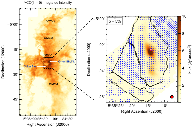
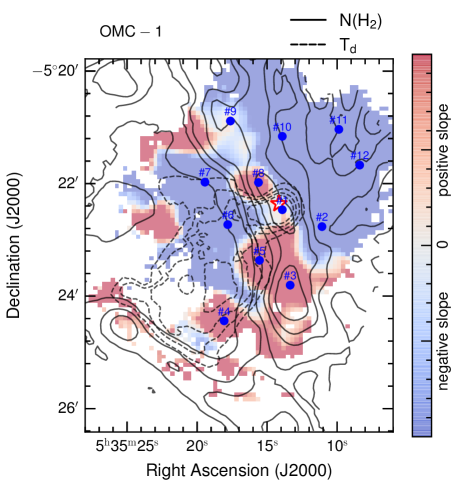
Figure 1: Left The map showing the intensity of ¹²CO(1-0) integrated over the OMC A cloud, which is bounded by OMC-3 in the north and OMC-4 in the south. The focus region in this study is indicated by the black box. Right Thermal dust polarization was observed at a wavelength of 54$\,\mu$m using SOFIA/HAWC+. The background color represents the total continuum intensity (Stokes-I). The blue segments indicate the orientation of the polarization (E-vectors), with their length indicating the degree of polarization. The black contour lines outline the Orion BN/KL, HII, and Bar. The red asterisk marks the location of the Orion BN/KL core. The CO data used in this study is obtained from the CARMA-NRO Orion Survey (Kong et al. 2018).

Figure 2: Spatial distribution of the spectral slope of the polarization spectrum in OMC-1. The reddish region shows a rising polarization spectrum, whereas the blueish region shows a spectrum with a falling slope. This map is overlayed with dust temperature (solid black lines with $T_{\rm d}\geq 60\,$K with a step of 5 K) and gas density (dashed black line with $N(\rm H_{2})=1,\,2,\,3,\,6,\,10,\,20\times 10^{22}\,\rm cm^{-2}$ or $A_{\rm V}\geq 12.4\,$magnitude). The blue dots indicate the 12 positions where the spectra are used to compare with numerical models.

Furthermore, Hoang et al. (2019) and Hoang (2019) showed that when exposed to a strong radiation field, large dust grains acquire a remarkably high angular velocity and the largest dust grains in the population cannot survive intact because the centrifugal force within a grain exceeds the binding energy that holds it together. This rotational disruption process is known as Radiative Torque Disruption (RAT-D). Extremely fast rotation of objects due to laser irradiation is demonstrated in laboratory experiments (e.g., Reimann et al. 2018; Ahn et al. 2018), and the disruptive effect of rotation is also seen in simulations (Reissl et al. 2023) and laboratory experiments (Holgate et al. 2019). As the RAT-D mechanism sets an upper limit on the size distribution of dust grains, it has implications for various aspects of dust astrophysics, including light extinction, polarization, and surface chemistry (see the review of Hoang 2020). The combination of RAT-A theory and the RAT-D mechanism, referred to as the RAT paradigm, has been shown to reproduce a wider range of dust polarization observations, extending to star-forming regions (see the review of Tram & Hoang 2022).

However, most interpretation of polarization data have been made based on data taken at a single wavelength or a combination of only a few wavelengths. To further validate the RAT theory, the next logical step is to synthesize the observed multiwavelength polarization, also known as the polarization spectrum predicted by the RAT theory, and confront it with observational data. Previous observational analyses (see, e.g., Gandilo et al. 2016; Shariff et al. 2019 and references therein) have shown that the slope of the polarization spectrum can vary locally within an interstellar cloud. In a recent study, Michail et al. (2021) used observations made in four bands of High-resolution Airborne Wideband Camera Plus (HAWC+) on board of the Stratospheric Observatory for Infrared Astronomy (SOFIA) centered at 54, 89, 154, and 214$\,\mu$m toward Orion Molecular Cloud 1 (OMC-1) in the Orion A cloud. They found that the slope decreases in cooler regions and increases in warmer regions.

Fanciullo et al. (2022) attempted to interpret the observed data in the NGC 2071 star forming region using the modeling approach introduced in Guillet et al. (2018). However, they found that the models were unable to accurately reproduce the observations, even when incorporating parameter variations. Other studies on multiple dust polarization observations in various clouds have reported a ”V-shape” in the spectra (e.g., Hildebrand et al. 1999; Vaillancourt et al. 2008; Vaillancourt & Matthews 2012), where the polarization degree initially decreases with wavelength and then increases with longer wavelengths. To understand these observations, Hildebrand et al. (2000); Seifried et al. (2023) have suggested the need to consider multiple dust components with different temperatures and alignment efficiencies along the line of sight. In the latter work, the authors emphasized that grain composition plays a significant role in determining the V-shape.

In this study, we revisit the polarization spectrum in OMC-1 as shown in Figure 2, which hosts dense molecular material (the Kleinmann-Low nebula) and a dense photodissociation region (the Orion bar). We refer to Genzel & Stutzki (1989) for a complete overview. This well-studied environment provides an excellent opportunity to study the physics of magnetically aligned grains in various physical conditions. Our objective is to quantitatively compare the predicted polarization spectrum based on the RAT paradigm with the observed data from the far-infrared (53, 89, 154, and 214$\,\mu$m) reported in Michail et al. (2021) to submillimeter wavelengths (450 and 850$\,\mu$m) reported in Hwang et al. (2021).

The structure of this paper is as follows. Section 2 presents our analysis of the multiwavelength thermal dust polarization observations. We discuss the interpretation of the observed spectra using the RAT paradigm in Section 3. Finally, our discussions and conclusions are provided in Sections 4 and 5, respectively.

2 Observed Polarization Spectrum

2.1 Ancillary Data

In this study, we utilized the thermal dust polarization data obtained from the HAWC+ camera onboard the SOFIA and the POL-2 polarimeter installed on the James Clerk Maxwell Telescope (JCMT). The SOFIA/HAWC + observations at wavelengths 54, 89, 154, and 214$\,\mu$m were previously reported in Chuss et al. (2019), while the JCMT/Pol-2 observations at 450 and 850$\,\mu$m were published in Hwang et al. (2021). To ensure consistency, we applied a smoothing process using convolution kernels to all Stokes I, Q and U maps with the largest full width at half maximum (FWHM) value of $18\hbox to0.0pt{.\hss}^{\prime\prime}2$. Subsequently, we re-gridded all the smoothed images to a uniform pixel size of $4\hbox to0.0pt{.\hss}^{\prime\prime}55$. The degree, angle and respective errors of the debiased polarization were estimated following Appendix A.1. Spectra were extracted from spatial regions for which data were available for all wavelength bands. In addition, we added the data obtained during the APEX/PolKA commissioning observations at 870$\,\mu$m (Wiesemeyer et al. 2014) to the spectra for comparison only and excluded these data points from the adjustment process in this study.

2.2 Polarization Spectra

At each wavelength, we first computed the average $p(\%)$ at each pixel within a two-beam kernel and then created the $p(\%)$ maps and the associated error before stacking them into a data cube. The spatial area of this data cube is defined by the condition that all six wavelengths must fulfill the circular beam, ensuring that the different data sets cover the same area of interest. Furthermore, the value of $p(\%)$ in the local pixel is set to null if the circular beam surface is filled less than 25% by the observed data.

To characterize whether the polarization spectrum increases or falls, we used a linear line to fit these spectra in each pixel, similar to that used by Michail et al. (2021), to determine the slope sign of the polarization spectrum. The resulting slope map can be seen in Figure 2. A positive (negative) value of the slope indicates an increase (decrease) in the polarization spectrum. We observe a rising spectrum (indicated by reddish colors) in the main filament structure of Orion and the Bar, while a falling spectrum (indicated by blueish colors) is observed elsewhere. In correlation with dust temperature and gas column density derived from the continuum dust SED fitting , it is observed that the increasing spectrum is closely correlated with dense gas, where dust temperature is not the hottest, except at the Orion BN/KL core.

In order to qualitatively compare observations and modeling, we used the average spectra over two beam sizes at 12 locations distributed throughout the OMC-1 region, as indicated by the blue dots in Figure 2. The resulting spectra and the corresponding slopes are shown in Figure 6, including error bars that represent the statistical error associated with the average kernel. It is evident that the shape and slope of the spectrum vary across the cloud, with some locations exhibiting a pronounced V-shape.

Table 1: The main input parameters of the modeling (radiation field and gas density) and the output parameters (maximum alignment efficiency cross the inclination angle of magnetic field and the size-distribution power index) from the best-fitting one-phase model. Besides, the maximum grain size is fixed as $2\,\mu$m, the mean wavelength of the field is fixed as $0.5\,\mu$m, and tensile strength is fixed as $10^{7}\,\rm erg\,cm^{-3}$.

One-phase Model
Regions	$U$	$n_{\rm H}\,\rm(cm^{-3})$	$f_{\rm max}\times\sin^{2}\psi$	$\beta$	$\chi^{2}$
#1	12099	$9.05\times 10^{5}$	0.80	-4.81	0.72
#2	555	$1.89\times 10^{5}$	0.33	-3.00	17.88
#3	372	$1.09\times 10^{6}$	0.08	-3.66	6.60
#4	5117	$3.09\times 10^{4}$	0.20	-3.14	4.17
#5	3153	$1.63\times 10^{5}$	0.31	-3.93	6.68
#6	7228	$5.16\times 10^{4}$	1.00	-3.85	6.88
#7	2403	$5.40\times 10^{4}$	0.75	-3.00	12.52
#8	857	$7.62\times 10^{5}$	1.00	-4.55	2.98
#9	52	$4.98\times 10^{5}$	0.13	-3.00	12.33
#10	184	$2.54\times 10^{5}$	0.29	-3.00	46.76
#11	59	$1.58\times 10^{5}$	0.42	-3.00	116.37
#12	45	$1.39\times 10^{5}$	0.45	-3.00	317.91

Table 2: Similar to Table 2 but for the two-phase model. The total and polarized emission in the second phase are scaled by $f_{\rm scale}$ and $f_{\rm heat}$ relatively to the first phase with $f_{\rm heat}=T^{\rm first-phase}_{\rm dust}/T^{\rm second-phase}_{\rm dust}$.

Two-phase Model
Regions	$f_{\rm max}\times\sin^{2}\psi$	$\beta$	$f_{\rm heat}$	$f_{\rm scale}$	$\chi^{2}$
#1	0.53	-4.50	2.14	6.85	0.56
#2	0.29	-3.53	3.06	39.89	10.73
#3	0.57	-4.00	2.13	181.46	3.41
#4	0.58	-4.23	1.53	60.42	2.15
#5	0.69	-4.37	1.24	104.03	2.61
#6	0.94	-4.22	5.37	39.67	5.29
#7	0.94	-4.17	3.42	31.25	3.74
#8	0.58	-4.20	1.70	11.42	2.53
#9	0.16	-3.00	1.84	161.87	2.30
#10	0.32	-3.37	2.50	113.48	16.33
#11	0.34	-3.00	2.35	36.86	18.00
#12	0.38	-3.02	2.31	40.52	26.19

3 Modeled Polarization Spectrum

3.1 One-phase Dust Model

We utilize a simplified model based on the RAT paradigm, as described in Lee et al. (2020) and updated in Tram et al. (2021). The model incorporates various input parameters that characterize local physical conditions (such as radiation field and gas density), grain properties (including size and shape), grain composition (such as silicate, carbonaceous, and mixtures), and grain compactness (tensile strength). It is worth noticing that our model accounts neither for depolarization caused by magnetic field fluctuation along the line of sight nor for the radiative transfer effects. In this work, we take into account the variation of the magnetic field by introducing a new parameter, which is the angle of inclination $\psi$ of the regular magnetic field to the sight line. This fluctuation causes depolarization, which reduces the degree of net polarization by a factor of $\sin^{2}\psi$. The fundamentals of our model are described in Appendix B.1.

Figure 4 visualizes the polarization spectrum predicted by our one-phase model. If only silicate grains are aligned, the degree of polarization decreases toward a higher wavelength. The polarization degree is higher in amplitude for the silicate and carbonaceous mixture, and the spectrum shows a plateau at a higher wavelength. One can see that the higher radiation field makes the spectrum rise at a shorter wavelength, and the degree is higher if the disruption effect is neglected (left panel) compared with the lower radiation field medium. In the case where the disruption effect is considered (right panel), the depletion of the largest grains for a sufficiently intense radiation field causes the polarization degree to decrease, which can be smaller than in the case of a low radiation field.

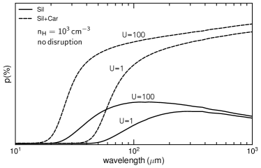
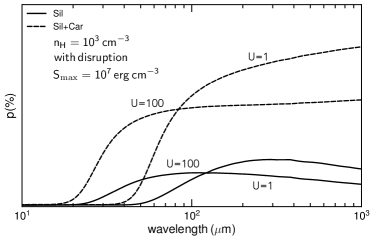
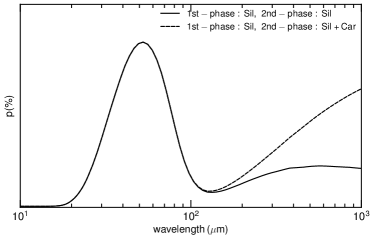
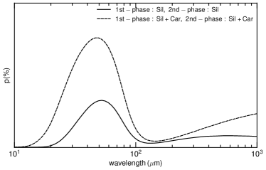
Figure 3: Polarization spectra predicted by our one-phase modeling for two radiation strengths of $U=1$ (i.e., the standard ISM radiation field) and $U=100$ (i.e., a hundred times higher than the standard ISM). Solid lines show the spectra for only aligned silicates, while dashed lines show the aligned silicate and carbonaceous mixture. The disruption by RAT-D is considered in the right panel for the composite grains with $S_{\rm max}=10^{7}\,\rm erg\,cm^{-3}$. For a demonstration, the value of $p(\%)$ is not shown.

Figure 4: Polarization spectrum predicted by our two-phase model. On the left, only aligned silicate produces polarization in the first phase (hot phase), while either aligned silicate (solid line) or aligned mixed silicate and carbonaceous (dashed line) in the second phase (cold phase) produce polarization. The right panel shows the case of mixed composition in the hot phase. This mixture increases $p(\%)$ in the hot phase and consequently shallows the V-shaped compared to that of only silicate showing in the left panel.

We used local values of dust temperature ($T_{\rm d}$) and gas column density ($N(\rm H_{2})$) that were fit to the spectral energy distribution of the dust (see Figure 2 in Chuss et al. 2019). Subsequently, we determined the local radiation intensity as $U\simeq(T_{\rm d}/16.4\,\rm K)^{6}$, where $U=u_{\rm rad}/(8.64\times 10^{-13}\,\rm erg\,cm^{-3})$ represents the ratio of the radiation density at the specific location to the radiation density in the surrounding area (Draine 2011). We estimate the density of the local gas volume as $n_{\rm H}=2\times N(\rm H_{2})/W$, where $W$ denotes the depth of the cloud. For OMC-1, $W\simeq 0.15\,$pc (see Pattle et al. 2017; Chuss et al. 2019), which is in agreement with the turbulent correlation length estimated in Guerra et al. (2021). In our model, two main parameters are varied: the product of the maximum alignment efficiency and the depolarization by magnetic field fluctuation ($f_{\rm max}\times\sin^{2}\psi$), and the power index of the grain size distribution ($\beta$). The adopted parameters can be found in Table 2.

We used LMFIT least square minimization, which extends the Levenberg–Marquardt method to restrict the best models, which were then used to fit the observed spectra. These fitted spectra are represented by the solid lines in Figure 6. The accuracy of the fitting is demonstrated in Appendix B.3. Our model is capable of reasonably replicating the observed spectra in certain regions, such as #1, #3, #4, #5, #6 and #8. However, our model does not fit the spectra well in other areas, leading to unconstrained parameters at those locations. Interestingly, the spectra that our model fails to reproduce exhibit a distinct ”V-shape” pattern.

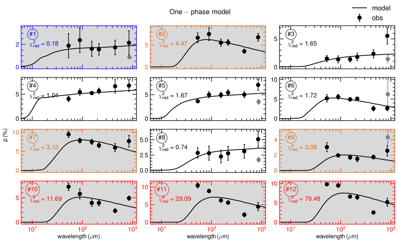
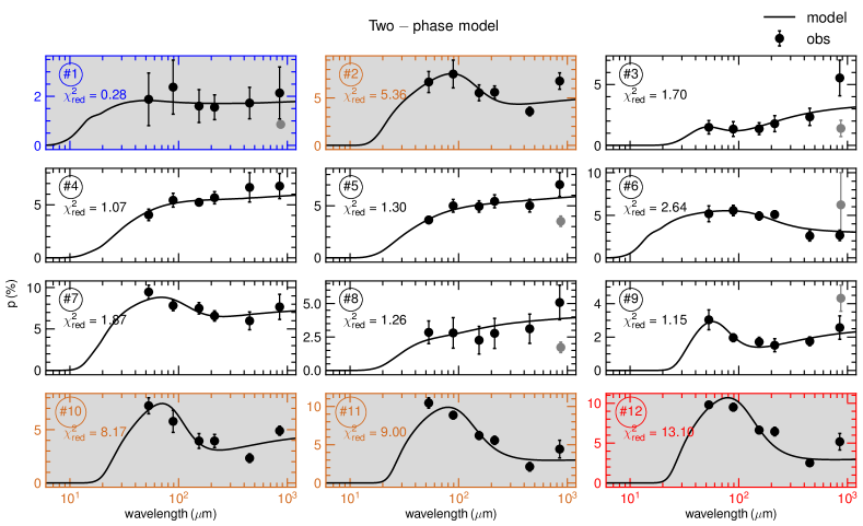
Figure 5: Polarization spectrum observed by SOFIA/HAWC+ and JCMT/Pol-2 (black dots) at 12 different locations in OMC-1 as shown in Figure 2 with the best one-phase model. The reduced chi-square ($\chi^{2}_{\rm red}$) indicates the ”good goodness” of the fit. The standard $\chi^{2}$ is shown in Table 2. For comparison, we show the APEX/PolKA observations at 870$\,\mu$m as a gray dot, but exclude them from the fitting. For visual guidance, we color the frame blue for $\chi^{2}_{\rm red}<0.5$, brown for $3<\chi^{2}_{\rm red}<10$, and red for $\chi^{2}_{\rm red}\geq 10$.

Figure 6: Similar to Figure 6 but with the best two-phase model. Compared to the one-phase model, the two-phase model significantly improves the quality of the fits, as illustrative by $\chi^{2}_{\rm red}$ or standard $\chi^{2}$ in Table 2. The presence of a cold dust layer is insignificant in #1, #4, #5, and #8, while the model cannot reproduce the V-shaped spectrum with a sharply rising slope in #2, #3, and #12.

3.2 Two-phase Dust Model

As previously mentioned, the polarization spectrum exhibits a ”V-shape” pattern, which cannot be accurately reproduced by the one-phase model. This phenomenon has been commonly observed in the literature (see, e.g., Hildebrand et al. 1999; Vaillancourt et al. 2008; Vaillancourt & Matthews 2012), and it is believed that multiple dust components are required along the line of sight (Hildebrand et al., 2000; Seifried et al., 2023). In the case of OMC-1, a 3D dust map of OMC-A reconstructed by Rezaei Kh. & Kainulainen (2022) has revealed the presence of multiple dust layers. Therefore, we have updated our one-phase model to a two-phase model, consisting of one warm layer and one cold layer, following the procedure outlined in Seifried et al. (2023). The governing equations for estimating the total and polarized intensities are essentially the same as those for the first layer. However, the relative contribution of the two phases to these intensities is parameterized by $f_{\rm scale}$, and the relative difference in the dust temperature (radiation field) is parameterized by $f_{\rm heat}$. We have made the critical assumption that the grain size distribution is identical in both phases and therefore we have varied four parameters ($f_{\rm max}\times\sin^{2}\psi$, $\beta$, $f_{\rm scale}$, and $f_{\rm heat}$). The details of the two-phase model are described in Appendix B.2.

Figure 4 shows the two-phase model predictions. In general, this model canreproduce the observed V-shape polarization spectrum. Moreover, a mixture of silicate and carbonaceous in the second phase results in a steep continuous increase of $p(\%)$ toward longer wavelengths (longer than 1 mm), thus making the spectrum’s V-shaped more pronounceable. On the contrary, the model with only aligned silicate grains causes $p(\%)$ to increase before decreasing in the millimeter range. It should be noted that, in the first phase, the shape of the spectrum is invariant, whether the alignment of only silicate or mixture to carbonaceous is considered, yet $p(\%)$ is higher for a mixed dust composition.

The lower panels depicted in Figure 6 exhibit the most accurate representations of the observations achieved by utilizing the two-phase model. The convergence of the fit is shown in Appendix B.3. The most optimal values for the parameters of this model can be found in Table 2. Compared with the one-phase model, the fit quality is generally improved from a statistical perspective, and the two-phase model successfully reproduces the V-shaped pattern observed in the spectra. We note that the contribution of a cold dust layer is minimal in regions #1, #4, #5, and #8, and the model encounters difficulties in accurately reproducing the V-shaped spectrum with a steeply increasing slope in regions #2, #3, and #12.

4 Discussions

4.1 Variation of Magnetic Fields at Different Wavelengths

We qualify the variation of the magnetic field variation on the plane of the sky within the main-beam by the dispersion function $S$ (introduced in Planck Collaboration et al. 2020) and turbulent parameter $F_{\rm turb}$ (introduced in Hoang & Truong 2023). We refer to Appendix A.2 for the details of formulations. The maps of $S$ and $F_{\rm turb}$ for all wavelengths are shown in Figures 8 and 8.

With a convolved FWHM of $18\hbox to0.0pt{.\hss}^{\prime\prime}2$, it is clear that the turbulence in the magnetic field is insignificant in most chosen regions, where it is defined by $F_{\rm turb}=1$. However, the variation is strongest at the location of the bar (not included in this study due to lack of available data), the BN/KL core (region #1) and around the region #3. It is noteworthy that there are new areas with significant fluctuations in magnetic fields at submillimeter wavelengths, which differ from those observed at far-infrared wavelengths and may support the idea of other layers of dust along the line of sight.

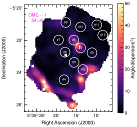
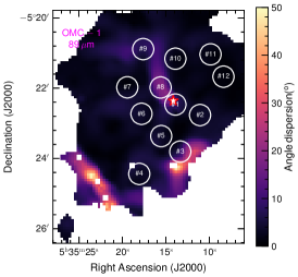
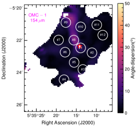
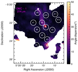
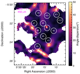
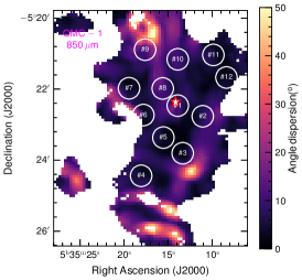
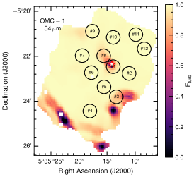
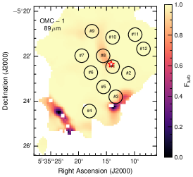
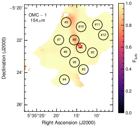
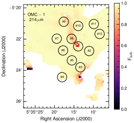
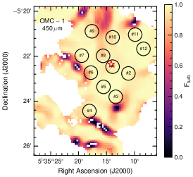
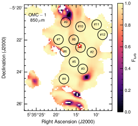
Figure 7: The angle dispersion is observed across all wavelengths. Analysis of submillimeter data indicates that the turbulence areas differ from those seen in the far-infrared data.

Figure 8: Similar to Figure 8 but for the turbulent parameter $F_{\rm turb}$. The condition Fturb = 1 indicates the absence of turbulence in the magnetic field, while greater turbulence results in a decreased value of $F_{\rm turb}$.

4.2 Footprint of Foreground/Background Components

At certain locations (regions #2, #3, #6, #7, #9, #10, #11, and #12 in Figure 6), the observed polarization spectrum displayed a V-shaped pattern. Our model, which incorporates two-phase dust (warm and cold phases) at these locations, was able to accurately reproduce these observations. The V-shaped polarization spectrum could potentially indicate the presence of a cold foreground or background cloud along the observed sight line, as the second phase in our model can exist either in front of or behind the first phase. We propose that utilizing multiple-wavelength thermal dust polarization observations could serve as a valuable tool for detecting multicomponent dust. This approach offers greater sensitivity compared to examining the total intensity SED. The primary underlying cause stems from the fact that, while the overall intensity in the cold phase is outshone by the SED of the hot phase, it is feasible to differentiate the cold layer, as long as grain alignment is effective, leading to a sufficiently high level of induced polarization.

It is important to mention that the fits obtained from the two-phase model exhibit similarities with the fits obtained from the one-phase model in regions #1, #4, #5, and #8. This similarity suggests that the second phase has a minimal contribution in these regions and implies that the background/foreground is a non-uniform distribution and varies along different sight lines toward the OMC-1 cloud.

4.3 Potential Evidence for Mixing Compositions of Dust Grains

Based on our most appropriate model, it was observed that polarization generation is caused by a mixture of silicate and carbonaceous grains in the cold phase (second phase). As grains could grow efficiently through accretion of metals to grains at a typical density of $\sim 10^{3}\,\rm cm^{-3}$ (Hirashita 2000) and metal depletion is greater in cold medium (Savage & Sembach 1996) or coagulation at a higher typical density of $\gtrsim 10^{3}\,\rm cm^{-3}$ (Stepnik et al. 2003), the mixture in grain composition could potentially be the result of grain growth under cold conditions.

It is crucial to mention that due to the degeneracy of the free parameter $f_{\rm scale}$, the model cannot distinguish between different grain compositions (whether silicate alone or carbonaceous in combination) in the first (warm) phase. However, we observed that the model with only silicate composition in the first phase completely fails to reproduce the observed spectra in the regions #2, #6 and #7.

4.4 Constraining the 3D Magnetic Field Structure from Dust Polarization

In our numerical modeling above, we combined the maximum alignment degree and the inclination angle of B-fields into one term, $f_{\rm max}\times\sin^{2}\psi$, and obtained the best-fit parameter for this product. However, we neglected the impact of variations in the magnetic field orientation along the sight line and within the main beam area (magnetic field tangling).

Here, we discuss the possibility of probing the B-field’s inclinations angle $\psi$ based on the best-fit value of the product $f_{\rm max}\times\sin^{2}\psi$. According to Magnetically enhanced RAT (MRAT) alignment theory, grains with embedded iron inclusions can achieve maximum alignment of $f_{\rm max}=1$ (Hoang & Lazarian, 2016). The existence of such superparamagnetic grains has been evident from numerous comparisons between numerical models and observations, either using Planck (Hensley & Draine 2023) or ALMA (Giang et al. 2023). Therefore, if we assume the most likely model with $f_{\rm max}=1$, we can infer the the B-field inclination angle based on the best-fit values. The results for $\psi$ angles are shown in Table 3.

In general, the value of the magnetic field inclination $\psi$ varies in OMC-1 locally. However, this variation is insignificant in the regions west of the main filament (#2, #10, #11, #12), and along the main filament (#1, #3, #8) except #9 where the gas density is lower than in others. Furthermore, it is interesting to note that this angle seems to decrease from the HII region (east of the main filament) to the main filament and further west of the main filament. Therefore, it suggests that we have a bow-shaped structure of the magnetic field that curves around the filament in OMC-1. The complete mapping of the angle $\psi$ could potentially reveal the three-dimensional structure of the magnetic field in OMC-1. We note that this approach is already tested using synthetic polarization of MHD simulations in Hoang & Truong (2023), but it is the first time applied to the observational data in this paper.

Table 3: The inclination of the magnetic field with respect to the line of sight in the case of $f_{\rm max}=1$ for the two-phase model.

Determination of 3D magnetic field from thermal dust polarization
Regions	$f_{\rm max}\times\sin^{2}\psi$	$\psi(^{o})$	location
#1	0.53	46.72	Main filament
#3	0.57	49.02	Main filament
#8	0.58	49.6	Main filament
#9	0.16	23.58	Main filament
#5	0.69	56.17	HII-filament border
#4	0.58	49.60	HII (East to filament)
#6	0.94	75.8	HII (East to filament)
#7	0.94	75.8	HII (East to filament)
#2	0.29	32.58	West to filament
#10	0.32	34.45	West to filament
#11	0.34	35.67	West to filament
#12	0.38	38.06	West to filament

4.5 Caveats

The polarization spectrum towards OMC-1 was constructed using observations from SOFIA/HAWC+ and JCMT/Pol-2. However, our work is subject to various uncertainties, both in terms of observations and computations. The rising slope of the V-shape in Figure 6 is mainly influenced by two observable data points at 450 and 850$\,\mu$m. In certain regions (e.g., regions #2, #3, and #12), the dust polarization at 850$\,\mu$m is relatively high, resulting in a steep slope towards longer wavelengths. This discrepancy reduces the goodness of fit in these specific regions. To verify this, we compared the 870$\,\mu$m observations and found a discrepancy with the 850$\,\mu$m observations. Therefore, it is crucial to conduct further observations at submillimeter wavelengths (e.g., APEX/A-MKID at 350 and 870$\,\mu$m) and millimeter wavelengths (e.g., IRAM/NIKA-2 at 1.2 mm) to improve the precision of the dust polarization spectrum. Furthermore, data from SOFIA/HAWC+ and JCMT/POL-2 were processed using different pipeline reductions. These variations in the reduction process could introduce biases in the resulting polarization degree. It is necessary to develop a consistent procedure for reducing data obtained from different telescopes. As demonstrated in this study, SOFIA/HAWC+ and JCMT/POL-2 observe dust polarization from different layers along the line of sight. However, it is also possible that there is an additional large-scale magnetic field component present in the SOFIA/HAWC+ observations, which causes the differences between these two observations. A further uncertainty results from the instrumental sensitivity of the polarization degree to the removal of sky backgrounds.

Our simplified model contains certain uncertainties. First, the model relies on locally observed physical properties of the environment, such as gas density and dust temperature. Therefore, these values are subject to change when a higher spatial resolution is considered. Second, our investigation focuses only on the parameter space of the most important parameters ($\beta$, $f_{\rm max}$, $\beta$, $f_{\rm heat}$, and $f_{\rm scale}$), while other parameters remain unexplored. For example, the dust-to-gas ratio (which we fixed at 1/100), the silicate/carbon ratio (which we fixed at 1.12 as in Draine & Lee 1984), and the composite grain tensile strength ($S_{\rm max}=10^{7}\,\rm erg\,cm^{-3}$). Different constrained best models may arise from variations in these parameters.

In addition, our assumption is that the emissions in the FIR/sub-mm range are optically thin in both cold and warm phases along the line of sight. Therefore, our model cannot accurately describe the radiative processes and their impact throughout these phases. To address this issue, a more accurate modeling approach can be utilized that incorporates a proper radiative transfer process and the RAT paradigm, such as POLARIS+ in Giang et al. (2023).

5 Conclusions

In this study, we presented the polarization of thermal dust emission in OMC-1 using data from four bands of SOFIA/HAWC+ (54, 89, 154, and 214$\,\mu$m) and two bands of JCMT/Pol-2 (450 and 850$\,\mu$m). In general, our analysis revealed that the slope of the polarization spectrum is positive along the main filament structure and the Orion Bar, where the gas density is relatively high. In regions with lower gas density, the slope is negative.

We compared our simplified model based on the RAT paradigm and accounted for the magnetic field fluctuation along the line of sight with the dust polarization spectra observed in OMC-1. Although the best-fit models were able to reproduce the observations reasonably well in some locations, they failed to explain the pronounced V-shape (the polarization degree first decreases and then increases toward a longer wavelength) observed in certain spectra. This V-shape suggests the presence of multiple dust layers along the line of sight, which is consistent with the findings of Rezaei Kh. & Kainulainen (2022). To improve our model, we introduced a ”two-phase” approach that accounts for two dust layers, and this modification resulted in a better fit to the observations across OMC-1. Our analysis also indicated that the dust polarization spectrum is more sensitive to the presence of multiple dust layers than the total intensity spectral energy distribution. Furthermore, the best-fit model suggested a composite composition of dust grains, consisting of a mixture of silicate and carbonaceous materials, in the cold dust layer.

We showed that the variations of the polarization angle on the plane of sky within the beam are distinct from submillimeter to FIR wavelengths. This discrepancy likely infers that FIR and submillimeter polarimetry probe different layers of dust along the light of sight. We discussed that if validated, combining the RAT-paradigm theories with the degree of dust polarization observations may allow inferring the local three-dimensional structure of the magnetic field along the individual line of sight.

We acknowledge that our study has uncertainties that arise from both the observations and the simplicity of our modeling approach. Nevertheless, our work emphasizes the importance of utilizing multiwavelength dust polarization to investigate the mechanisms of grain alignment and dust polarization, along with the effectiveness of the RAT paradigm in interpreting such polarization spectra.

Appendix A Observations

A.1 Synthesising data

In Section 2, we introduce that we worked on the polarization data at six distinct wavelengths. Thus, we synthesized all Stokes I, Q and U and their associated errors ($\sigma_{I}$, $\sigma_{Q}$, and $\sigma_{U}$) to a common FWHM of 18.2” and a pixel size of 4.55”. For the APEX/PolKA data, we applied the selection criteria of $I>0$, $I/\sigma_{I}\geq 10$, and $p/\sigma_{p}\geq 3$ and dentified only six regions that are covered by both PolKA and HAWC+ and POL-2. Subsequently, we computed the degree of polarization ($p(\%)$) as follows (see Gordon et al. 2018 for details).

The polarized intensity is defined as

$$I_{p}=\sqrt{Q^{2}+U^{2}}\leavevmode\nobreak\ \leavevmode\nobreak\ \leavevmode\nobreak\ .$$ (1)

Its associated error derived from error propagation, assuming that the errors in Q and U are uncorrelated, is

$$\sigma_{I_{p}}=\left[\frac{(Q\sigma_{Q})^{2}+(U\sigma_{U})^{2}}{Q^{2}+U^{2}}\right]^{1/2}\leavevmode\nobreak\ \leavevmode\nobreak\ \leavevmode\nobreak\ .$$ (2)

The debiased polarization degree and its associated error are calculated as

$$\begin{split}&p_{\rm biased}=\frac{100}{I}\sqrt{Q^{2}+U^{2}}\leavevmode\nobreak\ \leavevmode\nobreak\ \leavevmode\nobreak\ (\%),\\ &\sigma_{p}=p\left[\left(\frac{\sigma_{I_{p}}}{I_{p}}\right)^{2}+\left(\frac{\sigma_{I}}{I}\right)^{2}\right]^{1/2}\leavevmode\nobreak\ \leavevmode\nobreak\ \leavevmode\nobreak\ (\%),\\ &p=\sqrt{p^{2}_{\rm biased}-\sigma^{2}_{p}}\leavevmode\nobreak\ \leavevmode\nobreak\ \leavevmode\nobreak\ (\%),\end{split}$$ (3)

The polarization angle and its associated error are defined as

$$\begin{split}&\theta=\frac{90}{\pi}{\rm atan2}(U,Q)\leavevmode\nobreak\ \leavevmode\nobreak\ \leavevmode\nobreak\ (^{o}),\\ &\sigma_{\theta}=\frac{90}{\pi(Q^{2}+U^{2})}\sqrt{(Q\sigma_{U})^{2}+(U\sigma_{Q})^{2}}\leavevmode\nobreak\ \leavevmode\nobreak\ \leavevmode\nobreak\ (^{o}).\end{split}$$ (4)

A.2 Characterization of magnetic field tangling

The variation of B-fields could induce depolarization of thermal dust emission. Thus, we seek the relationship of the degree of polarization with the dispersion function $S$ of the polarization angle. The biased dispersion at position $\@vec{r}$ on the sight line is given as

$$S(\@vec{r})=\sqrt{\frac{1}{N}\sum^{N}_{i=1}[\theta(\vec{r}+\@vec{\delta}_{i})-\theta(\@vec{r})]^{2}}$$ (5)

and the associated error is (see Equation 8 in Planck Collaboration et al. 2020)

$$\sigma_{S}^{2}(\@vec{r})=\frac{1}{N^{2}S^{2}}\sum_{i=1}^{N}\sigma^{2}_{\psi}(\@vec{r}+\@vec{\delta_{i}})[\theta(\@vec{r}+\@vec{\delta}_{i})-\theta(\@vec{r})]^{2}+\frac{\sigma^{2}_{\theta}(\@vec{r})}{N^{2}S^{2}}\left[\sum_{i=1}^{N}\theta(\@vec{r}+\@vec{\delta}_{i})-\theta(\@vec{r})\right]^{2}$$ (6)

where $\theta(\vec{r})$ and $\sigma(\@vec{r})$ are the polarization angle and the associated error at position $\@vec{r}$, respectively. Similarly, $\theta(\vec{r}+\vec{\delta}$) and $\sigma(\@vec{r}+\@vec{\delta})$ for position $\@vec{r}+\@vec{\delta}$. $N$ is the number of angles chosen. In practice, for a given position $\@vec{r}$, we select all data points within a circle centered on this position with a diameter of two beam-size. Finally, the debiased dispersion function is computed as $\delta\theta=\sqrt{S^{2}-\sigma^{2}_{S}}$. The distribution of the dispersion angle is shown in Figure 8.

Another quantity that can qualitatively assess the turbulence in a magnetic field is $F_{\rm turb}$ introduced in Hoang & Truong (2023) as

$$F_{\rm turb}=\frac{1}{2}\left[3\langle\cos^{2}(\Delta\theta)\rangle-1\right]$$ (7)

with $\Delta\theta$ the deviation in the angle between the local magnetic field and the mean field. Furthermore, Hwang et al. (2021) showed that the OMC-1 region is sub-Alfvénic with a mean Alfvénic Mach number of approximately 0.4. Therefore, we can derive the link between $F_{\rm turb}$ and the angle dispersion as (see Eq. 32 in Hoang & Truong 2023)

$$F_{\rm turb}\simeq 1-1.5(\delta\theta)^{2}$$ (8)

The condition $F_{\rm turb}=1$ indicates the absence of turbulence in the magnetic field, while greater turbulence results in a decreased value of $F_{\rm turb}$. The distribution of $F_{\rm turb}$ for all wavelength is shown in Figure 8.

Appendix B Modeling

B.1 Recall the one-phase model basics

This study is based on the assumption of uniform ambient magnetic fields and does not take into account the radiative transfer. Thus, the total and polarized intensity can be estimated analytically, as described by Lee et al. (2020) and Tram et al. (2021). Our model is based on the theory of the RAT paradigm, and its basic concepts are briefly described below.

The degree of thermal dust polarization is defined as

$$p^{\rm ideal}(\%)=100\times\frac{I_{\rm pol}}{I_{\rm em}}\leavevmode\nobreak\ \leavevmode\nobreak\ \leavevmode\nobreak\ {.}$$ (9)

Where $I_{\rm pol}$ and $I_{\rm em}$ are the polarized and total intensity of the thermal dust emission. The depolarization due to the variation of the magnetic field along the line of sight can lower the polarized intensity and then reduced the net degree of the dust polarization as

$$p(\%)=p^{\rm ideal}(\%)\times\sin^{2}\psi\leavevmode\nobreak\ \leavevmode\nobreak\ \leavevmode\nobreak\ {.}$$ (10)

where $\psi$ is the mean angle of inclination of the regular magnetic field to the line of sight. If there is no component of the magnetic field on the sight line ($\psi=90^{0}$), the predicted $p(\%)$ is the maximum as $p^{\rm ideal}(\%)$.

As we only consider a dusty environment containing carbonaceous and silicate grains, the total emission intensity is

$$\frac{I^{\rm 1st-phase}_{\rm em}(\lambda)}{N_{\rm H}}=\sum_{j=\rm sil,car}\int^{a_{\rm max}}_{a_{\rm min}}Q_{\rm ext}\pi a^{2}\times\int dTB_{\lambda}(T_{\rm d})\frac{dP}{dT}\frac{1}{n_{\rm H}}\frac{dn_{j}}{da}da.\leavevmode\nobreak\ \leavevmode\nobreak\ \leavevmode\nobreak\$$ (11)

where $B_{\lambda}(T_{\rm d})$ is the black-body radiation at dust temperature $T_{\rm d}$, $dP/dT$ is the distribution of dust temperature, Q_ext is the extinction coefficient, $dn/da\sim a^{-\beta}$ is the grain-size distribution. As we work on the thermal dust polarization, we adopt the MRN-like distribution with the power index as a free parameter. The dust temperature distribution depends on the grain size and radiation strength, which is computed by the DustEM code (Compiègne et al. 2011, see, e.g., Figure 8 in Lee et al. 2020).

If silicate and carbon are separated populations, the silicates can align with the ambient magnetic field, while the carbon grains cannot. The polarized intensity is given by

$$\frac{I^{\rm 1st-phase}_{\rm pol}(\lambda)}{N_{\rm H}}=\int^{a_{\rm max}}_{a_{\rm align}}f(a)Q_{\rm pol}\pi a^{2}\times\int dTB_{\lambda}(T_{\rm d})\frac{dP}{dT}\frac{1}{n_{\rm H}}\frac{dn_{\rm sil}}{da}da,\leavevmode\nobreak\ \leavevmode\nobreak\ \leavevmode\nobreak\$$ (12)

$Q_{\rm pol}$ is the polarization coefficient and $f(a)$ is the alignment function. Size-dependent $f(a)$ is empirically described as

$$f(a)=f_{\rm max}\left[1-e^{-(0.5a/a_{\rm align})^{3}}\right]$$ (13)

with $a_{\rm align}$ the alignment size, above which grain is aligned. $f_{\rm max}$ is the maximum alignment efficiency. $f_{\rm max}=1$ stands for perfect alignment. It indicates that the grains with $a\geq a_{\rm align}$ align with an efficiency of $f_{\rm max}$, while the grains will not align otherwise. We varied the product of $f_{\rm max}\times\sin^{2}\psi$ as a free parameter. The alignment size $a_{\rm align}$ is determined by a condition in which the angular velocity obtained by RATs ($\omega_{\rm RAT}(a)$) is three times the thermal angular velocity ($\omega_{\rm th}$), which yields (see, e.g., Hoang et al. 2021 for the analytical formulations of $\omega_{\rm RAT}(a)$ and $\omega_{\rm th}$)

$$a_{\rm align}\simeq 0.055\left(\frac{\rho}{3\,\rm g\,cm^{-3}}\right)^{-1/7}\left(\frac{\gamma}{0.1}\right)^{-2/7}\left(\frac{n_{\rm H}}{10^{3}\,\rm cm^{-3}}\right)^{2/7}U^{-2/7}\times\left(\frac{T_{\rm gas}}{10\,\rm K}\right)^{2/7}\left(\frac{\bar{\lambda}}{1.2\,\rm\mu m}\right)^{4/7}(1+F_{\rm IR})^{2/7}\leavevmode\nobreak\ \leavevmode\nobreak\ \leavevmode\nobreak\ {\rm\mu m}$$ (14)

where $\rho$ is the volume mass density of grain, $\gamma$ is the degree of radiation anisotropy, $\bar{\lambda}$ is the mean wavelength of the radiation field, and $F_{\rm IR}$ is the ratio of the damping rate caused by infrared emission to the one caused by gas collisions.

If silicate and carbon grains are mixed (e.g., Jones et al. 2013), which may exist in dense clouds due to many cycles of photoprocessing, coagulation, shattering, accretion, and erosion, carbon grains could be passively aligned with the ambient magnetic field because of this mixture, and their thermal emission could be polarized. For the simplest case, assuming these grain populations have the same alignment parameters (i.e., $a_{\rm align}$, $f(a)$), the total polarized intensity is

$$\frac{I^{\rm 1st-phase}_{\rm pol}(\lambda)}{N_{\rm H}}=\sum_{j=\rm sil,car}\int^{a_{\rm max}}_{a_{\rm align}}f(a)Q_{\rm pol}\pi a^{2}\times\int dTB_{\lambda}(T_{\rm d})\frac{dP}{dT}\frac{1}{n_{\rm H}}\frac{dn_{j}}{da}da.$$ (15)

The extinction and polarization coefficients are calculated by the DDSCAT model (Draine & Flatau 1994, 2008; Flatau & Draine 2012) for a prolate spheroidal grain shape with an axial ratio of 1/3.

B.2 Two-phase model

We follow that approach in Seifried et al. (2023), the relative difference in intensities between the two phases is characterized by a factor $f_{\rm scale}$, the relative abundance between two phases is characterized by a factor $f_{\rm scale,car}$. The intensity of the radiation (equivalent to the temperature of the dust) in the second phase is related to that of the first phase as $f_{\rm heat}=T^{\rm 1st-phase}_{\rm d}/T^{\rm 2nd-phase}_{\rm d}$. In this simplified model, we made two critical assumptions. First, the power index of the distribution in the second phase is the same as in the first phase. Second, the total and polarized intensity are optically thin. With these assumptions, the total thermal dust intensity is a summation over two phases as

$$\begin{split}I^{\rm total}_{\rm em}&=I^{\rm 1st-phase}_{\rm em}+f_{\rm scale}\times\int^{a_{\rm 2,max}}_{a_{\rm 2,min}}Q_{\rm ext}\pi a^{2}\times\int dTB_{\lambda}(T^{\rm sil,2}_{\rm d})\frac{dP_{\rm sil,2}}{dT}\frac{1}{n_{\rm H}}\frac{dn_{\rm sil,2}}{da}da\\ &+f_{\rm scale}\times f_{\rm scale,car}\times\int^{a_{\rm 2,max}}_{a_{\rm 2,min}}Q_{\rm ext}\pi a^{2}\times\int dTB_{\lambda}(T^{\rm car,2}_{\rm d})\left(\frac{dP_{\rm car,2}}{dT}\right)\frac{1}{n_{\rm H}}\frac{dn_{\rm car,2}}{da}da.\leavevmode\nobreak\ \leavevmode\nobreak\ \leavevmode\nobreak\ \end{split}$$ (16)

If only silicate is considered to be aligned in the second phase, the total polarized intensity is

$$\begin{split}I^{\rm total}_{\rm pol}&=I^{\rm 1st-phase}_{\rm pol}\\ &+f_{\rm scale}\times\int^{a_{\rm max}}_{a_{\rm align}}f(a)Q_{\rm pol}\pi a^{2}\times\int dTB_{\lambda}(T^{\rm sil,2}_{\rm d})\frac{dP_{\rm sil,2}}{dT}\frac{1}{n_{\rm H}}\frac{dn_{\rm sil,2}}{da}da,\end{split}$$ (17)

If a mixture of silicate and carbonaceous grains are aligned, the total polarized intensity is then

$$\begin{split}I^{\rm total}_{\rm pol}&=I^{\rm 1st-phase}_{\rm pol}+f_{\rm scale}\times\int^{a_{\rm max}}_{a_{\rm align}}f(a)Q_{\rm pol}\pi a^{2}\times\int dTB_{\lambda}(T^{\rm sil,2}_{\rm d})\frac{dP_{\rm sil,2}}{dT}\frac{1}{n_{\rm H}}\frac{dn_{\rm sil,2}}{da}da\\ &+f_{\rm scale}\times f_{\rm scale,car}\times\int^{a_{\rm max}}_{a_{\rm align}}f(a)Q_{\rm pol}\pi a^{2}\times\int dTB_{\lambda}(T^{\rm car,2}_{\rm d})\frac{dP_{\rm car,2}}{dT}\frac{1}{n_{\rm H}}\frac{dn_{\rm car,2}}{da}da\end{split}$$ (18)

where the subscript and superscript number 2 refer to the second phase. In this work, we do not consider the variation in abundance of the carbonaceous grain between two phases and thus keep $f_{\rm scale,car}=1$ as a constant. Another practical reason for not varying $f_{\rm scale,car}$ is the degeneration of the fitting given 6 data points in the spectrum.

B.3 Modeling the polarization spectrum and fit to observations

As mentioned in Section 3, we constrained the best parameters using the least-square function of the LMFIT library in Python. We set the boundaries of $f_{\rm max}$ in the intervals [0.01, 1.0], $\beta$ of the intervals [-5.0, -3.0] and $f_{\rm scale}$ of the intervals [1, $10^{4}$]. To speed up the fitting process, we manually adjust the intervals of $f_{\rm heat}$ for different regions. For example, $f_{\rm heat}$ is set lower than 3 for the majority, except for regions #2, #6 and #7. Figure 9 shows an example of the conversion of the fit for the region #9 with the one-phase model (left panel) and the two-phase model (right panel). The two-phase model significantly reproduces the observed spectrum and significantly improves the goodness of fit. It is worth mentioning that we experience that the best fit is quite sensitive to the free $f_{\rm scale}$ and $f_{\rm heat}$ boundary (for example, the larger the boundary is set, the worse the fit is obtained). Thus, we narrowed these boundaries by running a serial test.

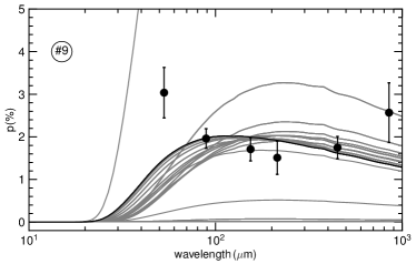
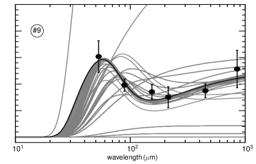
Figure 9: An example of the conversion of the least-square fitting procedure. The points are the data observed in #9 as in Figure 6. The solid gray lines are the modeling predictions with parameter variations. The solid black line represents the best fit of the data. The fitting of the one-phase model is in the left panel, while the two-phase model is in the right panel.