Sparse inference in Poisson log-normal model by approximating the -norm
Abstract
Variable selection methods are required in practical statistical modeling, to identify and include only the most relevant predictors, and then improving model interpretability. Such variable selection methods are typically employed in regression models, for instance in this article for the Poisson Log Normal model (PLN, Chiquet et al.,, 2021). This model aim to explain multivariate count data using dependent variables, and its utility was demonstrating in scientific fields such as ecology and agronomy. In the case of the PLN model, most recent papers focus on sparse networks inference through combination of the likelihood with a -penalty on the precision matrix. In this paper, we propose to rely on a recent penalization method (SIC, O’Neill and Burke,, 2023), which consists in smoothly approximating the -penalty, and that avoids the calibration of a tuning parameter with a cross-validation procedure. Moreover, this work focuses on the coefficient matrix of the PLN model and establishes an inference procedure ensuring effective variable selection performance, so that the resulting fitted model explaining multivariate count data using only relevant explanatory variables. Our proposal involves implementing a procedure that integrates the SIC penalization algorithm (-telescoping) and the PLN model fitting algorithm (a variational EM algorithm). To support our proposal, we provide theoretical results and insights about the penalization method, and we perform simulation studies to assess the method, which is also applied on real datasets.
Keywords Variable selection Multivariate count data Variational EM algorithm Information criteria Bayes estimate
1 Introduction
Multivariate count data analysis is an active component of modern statistical modeling, providing insights across various fields such as among others ecology, microbiology, and accident crash frequency. Unlike univariate count data analysis, multivariate count data analysis deals with multiple count variables simultaneously, capturing dependent aspects of the studied phenomena. Examples include studying the simultaneous abundance of various species in ecological communities, modeling the occurrence of different diseases in a population (Zhang et al.,, 2017), or the relative abundances of microorganisms in a specific ecosystem (Chiquet et al.,, 2018). Analyzing multivariate count data presents challenges, including handling dependencies among count variables, addressing over-dispersion, and accommodating complex correlation structures. In recent years, advanced statistical methods such as multivariate Poisson regression (PLN, Chiquet et al.,, 2021), multivariate negative binomial regression (Shi and Valdez,, 2014), and copula-based negative binomial models (Nikoloulopoulos and Karlis,, 2009) have been developed to tackle these challenges.
In this paper, we focus on the PLN model, which offers versatility for considering additional extensions (Chiquet et al.,, 2021), has demonstrated utility across various domains (Thierry et al.,, 2023; Grollemund et al.,, 2023), and continues to be studied computationally (Stoehr and Robin,, 2024). This model involves a latent layer, complicating inference, particularly computationally. Therefore, its implementation relies on variational approximation and the model is fitted using the Variational Expectation-Maximization algorithm (VEM), according to the R package PLNmodels. Nevertheless, it is practically feasible to fit this type of model using a Monte Carlo approach (Chib and Winkelmann,, 2001; Karlis and Xekalaki,, 2005; Stoehr and Robin,, 2024), or Laplace’s method to approximate the likelihood and to derive penalized maximum likelihood estimates (Choi et al.,, 2017).
Using the PLN model enables the study of network structures through estimated coefficients of the precision matrix in practical contexts. It also allows for investigating the impact of dependent variables on count data by estimating regression coefficients. In such cases, it is natural to design an estimation procedure coupled with a variable selection method to ensure that the fitted model retains only coefficients notably different from 0. This facilitates the interpretation of model coefficients, particularly when the primary interest is discerning dependent variables explaining heterogeneity in count data. For the PLN model, a variable selection procedure can be defined solely on the precision matrix coefficients, focusing on the major connections in a network analysis (Choi et al.,, 2017; Chiquet et al.,, 2019). Alternatively, a variable selection procedure can target only the regression coefficients, particularly when the precision matrix is not the coefficient of interest for addressing the specific issues of the field of application. Furthermore, it is also possible to penalize both the precision matrix and the regression coefficients, with the thought that the simplicity of the precision matrix can help achieve good performance in estimating regression coefficients (Wu et al.,, 2018; Rothman et al.,, 2010; Sohn and Kim,, 2012). In this paper, we focus on penalizing regression coefficients to interpret the selected coefficients, while most recent works emphasize sparse estimation of the precision matrix for network analysis.
To perform variable selection, the aim is to balance model fitting and the intensity of the -norm of coefficient parameters. Accepting a loss in model fitting can help to minimize the -norm, effectively turning off some coefficients. Thus, the aim is to adjust the model while minimizing this quantity, yet this leads to a mathematically or computationally complex optimization objective. To address this, a standard approach is to employ penalization (or its variants), which relaxes the optimization problem (Tibshirani,, 1996). Note that these methods typically involve a tuning parameter that drives the trade-off between model fitting and variable selection intensity. To numerically compute this tuning parameter, it is required to rely on an ad-hoc procedure, leading to computational overload that can be significant.
Recently, O’Neill and Burke, (2023) introduced a novel penalization approach aiming at approximating the -norm to achieve effective variable selection performance without requiring tuning parameter calibration through procedures like cross-validation. This approach is developed within the framework of a distributional regression model, enabling simultaneous assessment of covariate effects on both the mean and variance of the response variable. In this work, we propose to adapt this approach to the context of a PLN model, which is a generalized linear model whose inference is conducted using an EM algorithm and a variational approximation. In the following sections, we first recall the PLN model (see Section 2) and the variable selection procedure (see Section 3), and we provide additional theoretical insights and interpretation. Next, the main methodological contribution is presented in Section 4, in which we detail how to combine the variable selection algorithm proposed by O’Neill and Burke, (2023) (-telescoping Algorithm) with the PLN model inference proposed by Chiquet et al., (2021) (a VEM Algorithm). Then, the developed methodology is evaluated using real and simulated data in Sections 5 and 6.
2 Multivariate Poisson Log-Normal (PLN) Model
2.1 Model formulation
The multivariate PLN model was introduced by Aitchison and Ho, (1989) with the aim of modelling joint species count data using environmental factors, taking into account the dependency structure between species. In contrast to other multivariate Poisson models, the PLN model can handle data with a completely general correlation structure as well as overdispersion (Park and Lord,, 2007). Each observed count follows a Poisson distribution whose log parameter, defined on a latent layer, is distributed according to a multivariate Gaussian distribution. The expectation of this Gaussian distribution takes account of dependent variables, while its variance-covariance matrix characterizes the count data correlation structure. Let be the number of observations (or sites) assumed to be independent, and the number of features (or species) counted for each observation. We denote by the count matrix — where is the number of occurrences of the feature observed for the observation — and by the matrix of dependent variables. The fixed effect can be decomposed as , where is the vector of covariates for individual and is the vector of regression coefficients associated with feature . Finally, denotes the offset matrix, where the element is the offset of individual and feature , which represent the sampling effort varying from one individual to another and from one feature to another. The PLN model is then written as follows (Chiquet et al.,, 2021):
| (observed space) | (1) | ||||
| (latent space), |
where and . In the following, denotes the set of model parameters, where is the matrix of regression coefficients.
2.2 Parameters estimation
As the PLN model is a latent variable model, computing its log-likelihood is not straightforward and the use of the EM algorithm is required to estimate the parameters. However, to fit a PLN model, the EM algorithm assumes knowledge of the conditional distributions for each , which are intractable. Variational approximations have therefore been developed to circumvent this problem (Blei et al.,, 2017). The combination of variational approaches and the EM algorithm has led to the variational EM (VEM, Tzikas et al.,, 2008), which maximises a lower bound on the -likelihood of the PLN model. The VEM algorithm can be seen as minimizing the Kullback-Leibler (KL) divergence between and an approximate distribution chosen from a class of simple distributions. In most cases, is assumed to be a multivariate Gaussian distribution with expectation and variance-covariance matrix (Hall et al.,, 2011). All the variational parameters are gathered in , where and . The evidence lower bound (ELBO) of the log-likelihood which is maximized when implementing the VEM algorithm takes the general form (Blei et al.,, 2017):
| (2) |
In the case of the PLN model, the ELBO can be expressed as (Chiquet et al.,, 2021):
| (3) |
where is the Hadamard product and , is the precision matrix and its determinant, and is the matrix of expected count with entries , with the element of and the element of .
Typically, all the entries of parameters estimations of and of from will be non-zero. This will make model interpretation challenging if and are large. It is generally assumed that there is a "true model", characterized by a limited number of non-zero parameters and , facilitating interpretation and alleviating overfitting problems. To achieve this, it is necessary to impose constraints or regularization on the estimation process (Fan and Li,, 2001; Rothman et al.,, 2010; Hastie et al.,, 2015).
2.3 Sparse inference in Poisson log-normal model
Most studies on variable selection in the context of PLN models have focused on identifying dependency structures in the precision matrix. The main difference between these studies is the method used to compute the likelihood, but notice that they involve an penalty as a constraint on the log-likelihood.
Sparsity of the precision matrix. Choi et al., (2017) used the Laplace method to approximate the PLN log-likelihood, and imposed a constraint on the coefficients of precision matrix . They suggest that the penalized log-likelihood is:
where is the log-likelihood for observation and is a vector representing the mean parameter of a multivariate Gaussian distribution. The regularization is controlled by parameter and weights , the latter allowing differential amounts of penalty on the entries of based on prior knowledge or anticipated network properties. Next, Chiquet et al., (2019) focused on network inference and applied variational approximation methods to maximize a penalized lower bound of the log-likelihood in order to identify direct interactions among features. The corresponding objective function they suggest to maximize is defined as (Chiquet et al.,, 2018):
where is the ELBO (3), is the off-diagonal -norm of and is a tuning parameter controlling the amount of sparsity.
Sparsity of the coefficient matrix and the precision matrix. Wu et al., (2018) proposed a Monte Carlo EM algorithm for parameter estimation in the PLN model. To induce sparsity in the parameters, they imposed an constraint on both matrixes and . The penalized log-likelihood they maximize is defined as:
where is the log-likelihood of the PLN model, denote the matrix norm and , are two tuning parameters. Lastly, to our knowledge, there are no existing studies addressing sparse inference solely for the coefficient matrix in the case of the PLN model relying on variational approximation.
A remark on predicting on a validation dataset. In the aforementioned references, the best values of , and are selected by maximizing a pseudo-information criterion, either the BIC (Schwarz,, 1978) or its high-dimensional-adapted extension known as EBIC (Chen and Chen,, 2008), in which the true log-likelihood is replaced by an approximation. In standard practice, sparsity can also be reached thanks to a penalization method, for which it is essential to properly calibrate parameter , as it determines the trade-off between goodness of fit and intensity of penalization. Typically, is calibrated through cross-validation, by using a predefined sequence of values and assessing prediction performance on test data not used in the learning process. To predict count data values with PLN model, two formulas are available:
| (Variational PLN prediction) | ||||
| (PLN prediction) |
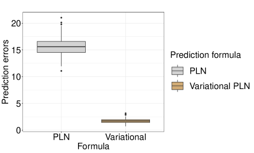
The first one involves variational parameters, while the other depends solely on PLN model parameters. It should be noted that the variational parameters are individual-specific, and to estimate the variational parameters of the -th individual, count data and covariates concerning the -th individual are required. Therefore, the formula involving variational parameters cannot be used to predict new data, which are not present in the training dataset. Additionally, an empirical study (see Section 5.2 and Figure 5) reveals that prediction performance of the formula without variational parameters is relatively weak compared to the other formula. Consequently, robust calibration of tuning parameter may not be achieved through cross-validation procedure. This limitation is an obstacle to the use of a penalization method requiring calibration of a tuning parameter, such as LASSO estimation.
3 Variable selection with SIC
Numerous variable selection methods have already been developed; we refer the reader to Heinze et al., (2018) for a recent review of the literature. Standard methods consist in regularizing the regression coefficients (for example, the LASSO (Tibshirani,, 1996) and its extensions (Zou,, 2006)), or to optimize an information criterion (such as AIC (Akaike,, 1974) or BIC (Schwarz,, 1978)). Unfortunately, in practice, these methods can be computationally intensive: LASSO-type methods require the intensity of the regularisation to be calibrated by cross-validation, while AIC/BIC-type methods require a very large number of models to be fitted. Recently, a penalization method called Smooth Information Criterion (SIC, O’Neill and Burke,, 2023) was introduced in order to achieve variable selection using a numerical procedure with reduced computational cost. It is based on an approximation of the -norm of the regression coefficients, so that it offers a relaxed version of BIC. It is expressed as a penalized -likelihood by:
| (4) |
where denotes a log-likelihood depending on parameter , is a sub-vector of corresponding to the parameters to be regularized, is an approximation of the -norm (see section 3.1) and is the number of the unpenalized parameters.
This approach simplifies the model selection process by avoiding to estimate the model coefficients for different values of a tuning parameter , or to fit many models for evaluating each of them with regards to an information criterion (O’Neill and Burke,, 2023). In other words, this method enables variables to be selected in a single step, eliminating the need to calibrate a regularization parameter by cross-validation. This new variable selection method seems advantageous in the case of the PLN model, since a cross-validation procedure is challenging to implement in this context. However, the proposed method do not avoid the use of an iterative algorithm to fit the model, although the procedure is numerically less costly. The specific iterative algorithm called -telescoping involves varying the form of the penalty, to smoothly approximate the -norm in order to ensure robust results (see Section 3.1.1 for a few details or O’Neill and Burke, (2023) for a complete description).
3.1 Formulations and interpretations
3.1.1 Optimization framework
In order to provide valuable insights in Section 3.1.2 and Section 3.1.3, we firstly present below the SIC approach in the context of a Multiple Linear Regression model:
| (5) |
where is the response for individual , the vector of covariates, and the vector of regression coefficients. In the following, we consider that the covariates are centered and reduced and we assume that , where the variance is known. In this context, the SIC procedure targets the solution to the optimization problem:
| (6) |
where , with
| (7) |
Note that can be seen as a smooth approximation of the -norm since . Moreover, the constrained minimization problem (6) can be written in the so-called Lagrangian or penalized form:
| (8) |
where the shrinkage parameter in (8) is in bijection with the radius in (6).
For a Generalized Linear Model, statistical inference relies usually on maximizing the likelihood function. To obtain sparse parameters in this context, the penalized maximum likelihood method can be used (Fan and Li,, 2001; Tibshirani,, 1996) and we denote the -likelihood of Model (5) by . Then the penalized log-likelihood involving SIC can be written as:
where is the number of unpenalized parameters (here, ) and is fixed at or for AIC and BIC respectively. The parameters maximizing the penalized log-likelihood are obtained using an iterative algorithm such as Newton-Raphson or Fisher scoring.
The Smooth Information Criterion depends on parameter , which influences the way variables are selected. Small values of lead to a better approximation of the -norm, but induce instability in the estimation process. Conversely, large values of provide a stable estimation process, but do not allow some coefficients to be set to zero because the level of shrinkage is too low. O’Neill and Burke, (2023) propose an algorithm, called -telescoping, which stabilises the variable selection by iteratively decreasing the values of in the optimization problem. As tends towards 0 in this algorithm, and a small implies that the approximation function is close to the -norm, the estimators are encouraged to be sparse at the end of the procedure.
3.1.2 Geometry of SIC
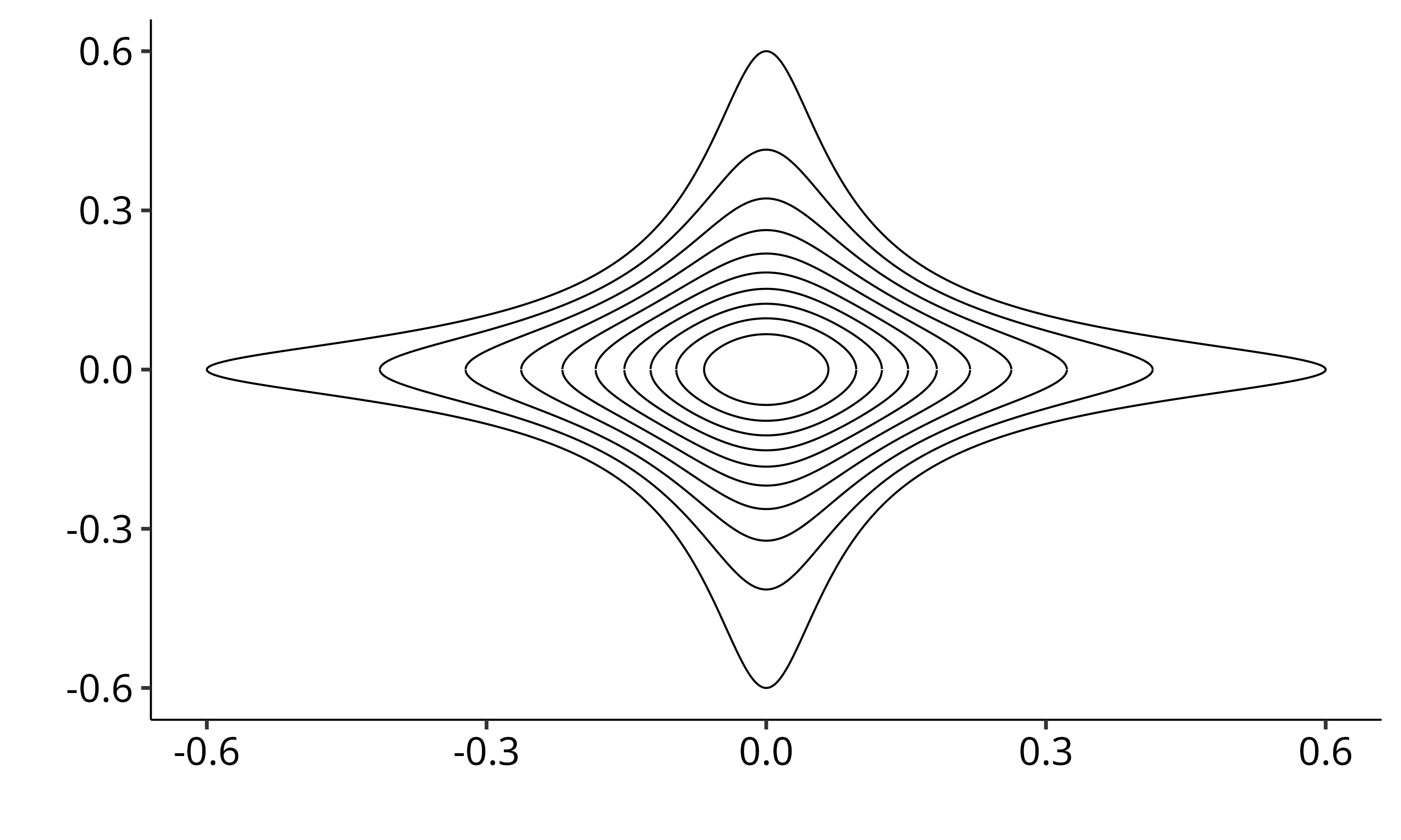
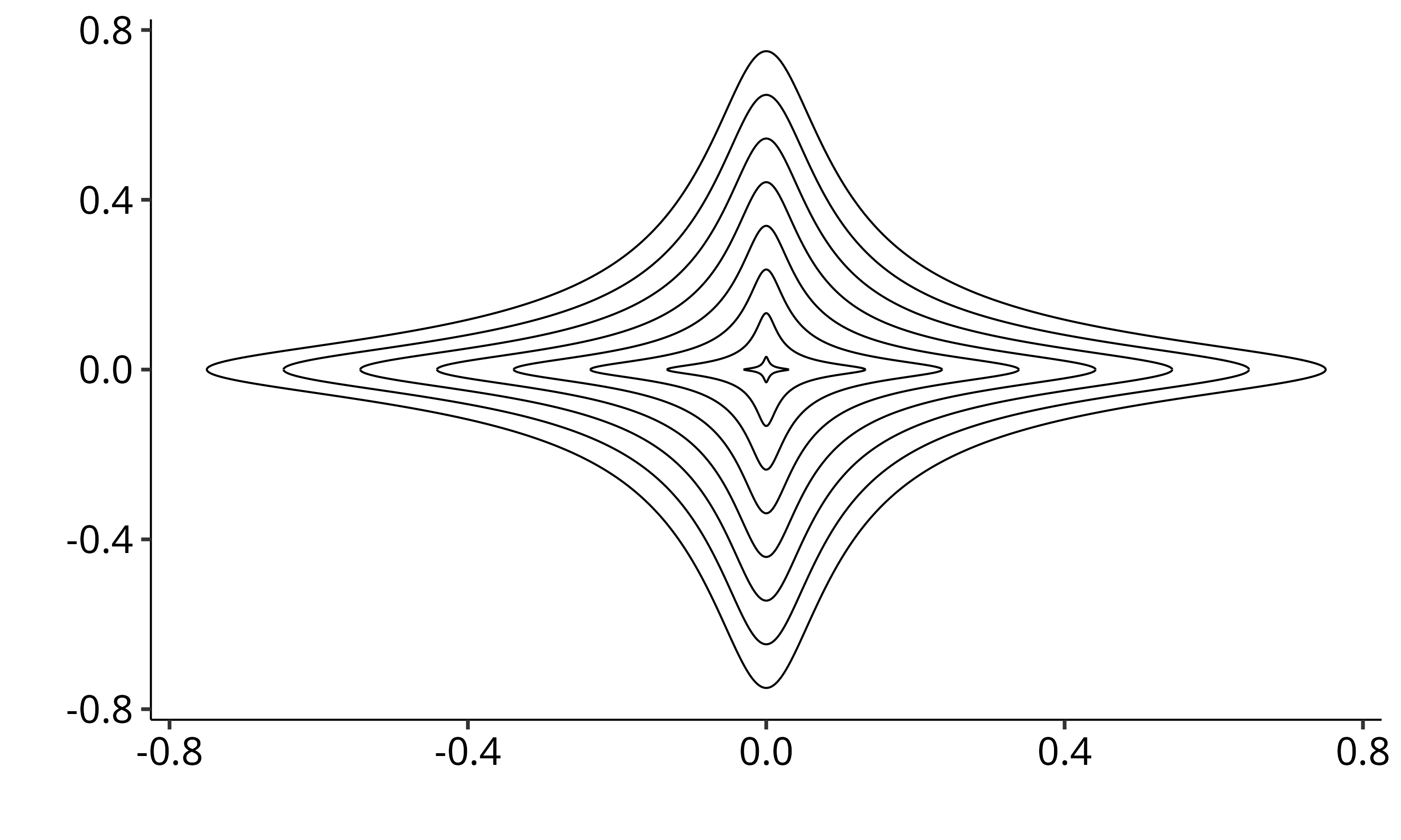
In what follows, for simplicity, function is treated as a norm, although it is not the case. Indeed, is not a norm since it does not satisfy the property of absolute homogeneity because , and in particular : . Notice that "-norm" is also a misnomer as it does not respect the property of absolute homogeneity either. To provide additional insights into the interpretation of SIC, we present two plots depicting the balls related this penalty. The left plot in Figure 1 shows contour lines of a ball, for different radius and for a fixed . The right plot illustrates contour lines of different balls with same radius as decreases. Mathematical details are given in Appendix A.
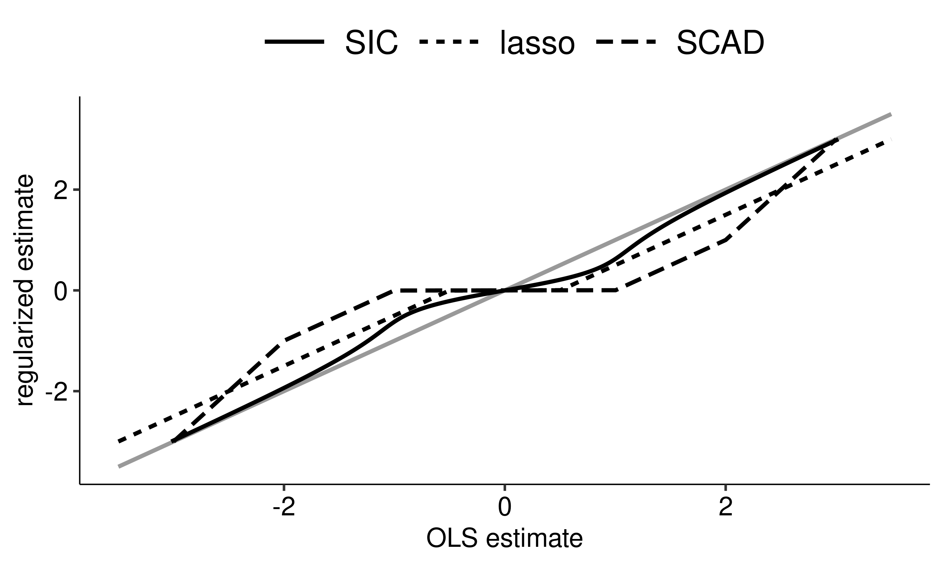
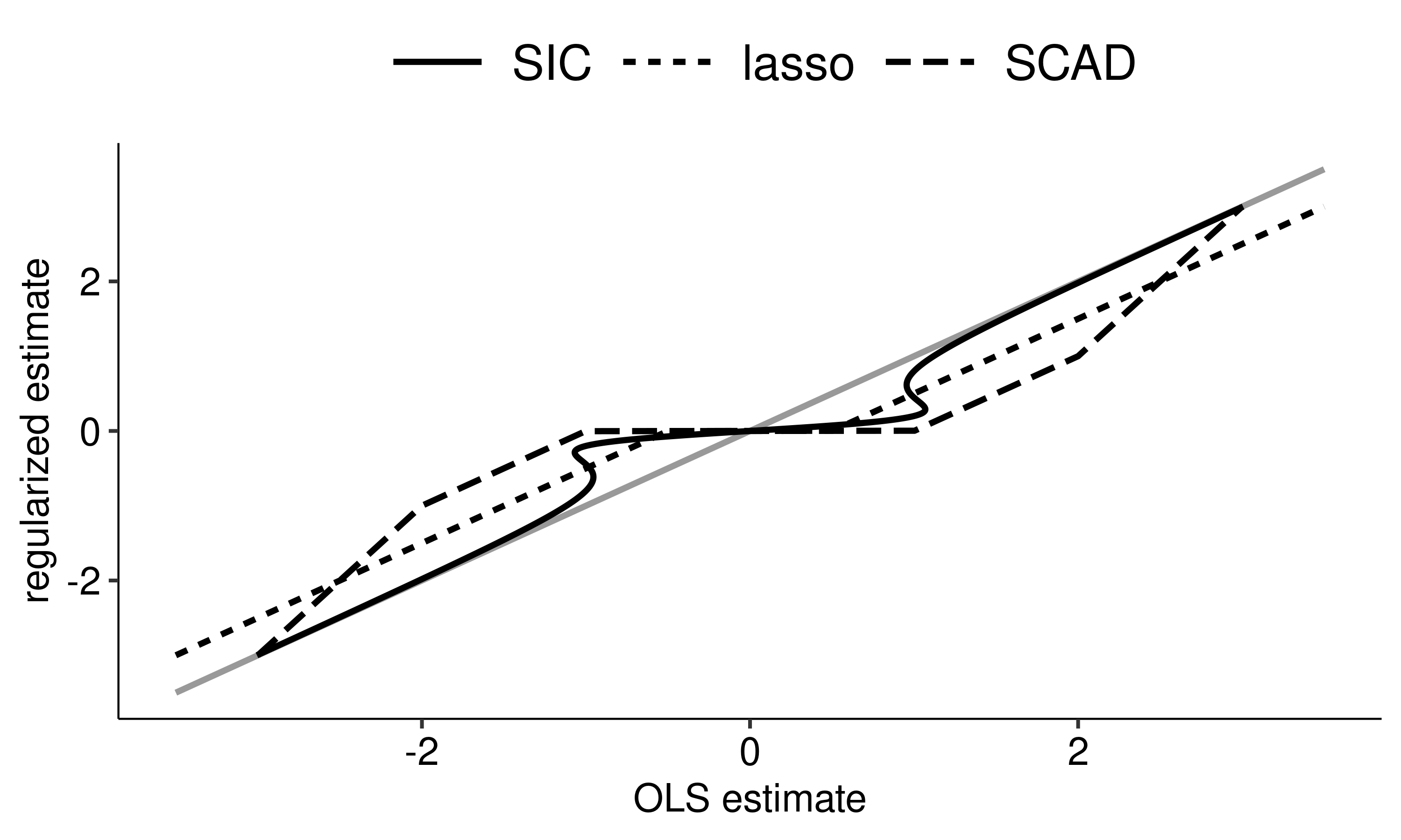
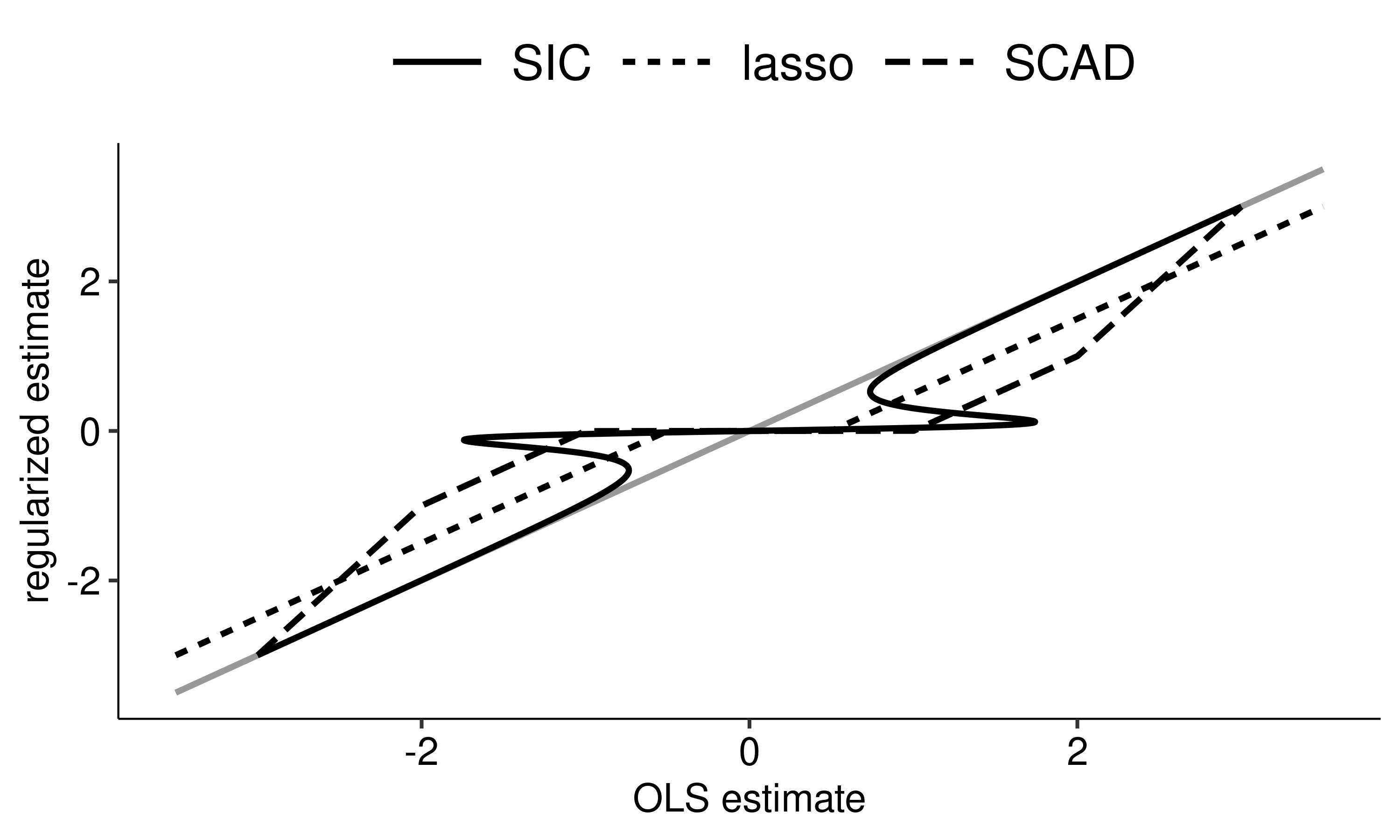
To compare the SIC penalization with other well-known penalization methods such as LASSO (Tibshirani,, 1996) or SCAD (Fan and Li,, 2001), it can be interpreted as a soft-thresholding rule. To illustrate with a simple yet informative plots, consider a model on , where and where the design is supposed to be orthonormal, so that coincides with the OLS estimate of for Model (5). For what follows, according to Fan and Li, (2001), tThe Gaussian white noise model is assumed for , so that , where . Therefore, using the SIC approach to estimate the ’s leads to the minimization of the following criterion:
Note that minimizing this criterion reduces to minimizing it component by component, leading to the equation:
Equations related to LASSO and SCAD penalizations can be determined in a similar way, and all these conditions are depicted in Figure 2, which helps understanding the bias induced in the OLS estimator by adding such penalization terms. For instance, it is observed that SIC penalization exhibits an interesting property, similar to SCAD penalty: for large OLS estimator values, the penalization does not induce bias on the estimator (unlike LASSO penalty). Moreover, it can be observed from Figure 2 that when is close to 0, the perturbation of the OLS estimator does not have a unique solution. This is related to the instability induced by this penalization, as previously identified by O’Neill and Burke, (2023), which justified the use of the -telescoping algorithm to ensure a robust estimation procedure.
3.1.3 SIC as Bayes estimate
The prior distribution related to the SIC penality. Penalization methods in Gaussian regression models can be interpreted in a Bayesian context. For example, Ridge penalization corresponds to the MAP estimate associated to a Gaussian prior, while LASSO penalization corresponds to a Laplace prior (Park and Casella,, 2008). Similarly, SIC estimators can be obtained as the Bayesian MAP estimate of for the prior :
| (9) |
where
This can be seen by noting that the estimator obtained by maximising (8) can be represented as
| (10) |
When goes to , converges to the constant . Therefore is an improper distribution whose tail is equivalent to that of a flat prior. The posterior distribution is
which is proper when is a full-rank matrix.
Two additive components and interpretations. To get a better understanding of the prior , let decompose into two additive parts: a flat prior and a proper prior denoted and defined by
| (11) | ||||
| (12) |
where Equation (12) is obtained since and where is the normalizing constant:
Up to the scalar factor , the prior can be reformulated as
| (13) |
See Figure 3 for a visual representation of the prior distribution and its two components.
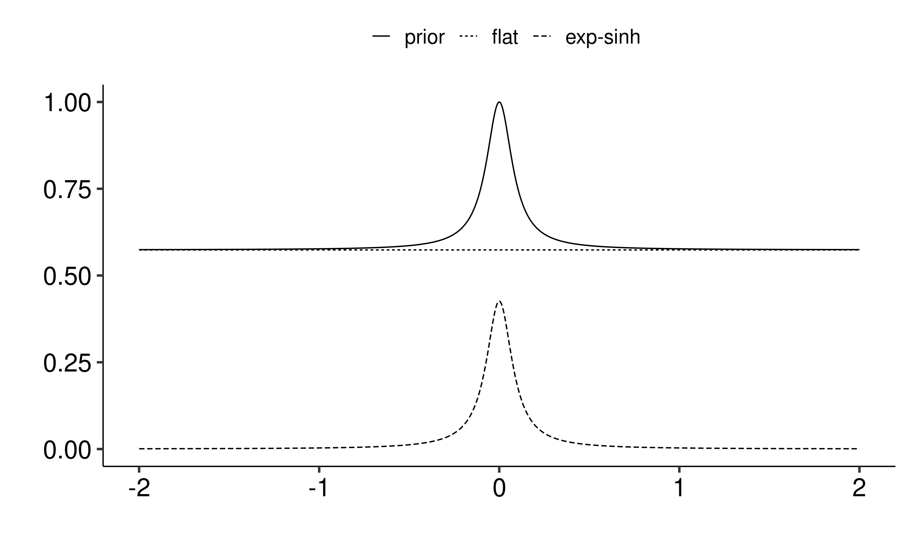
The scalar appears as the relative weight between the flat distribution and the proper distribution . To see that is proper and therefore that is well defined, we note that the tail behaviour of is equivalent to which is integrable. Note that can be seen as a smoothed approximation of , the Dirac measure in 0, for large values of . Indeed, it can be shown that converges narrowly to as goes to . So, the prior has some similarity with another prior distribution consisting of two additive components: the prior used in the spike and slab regression (Mitchell and Beauchamp,, 1988; Ishwaran and Rao,, 2005) where the heavy tailed distribution is replaced by a flat prior and the Dirac measure is approximate by .
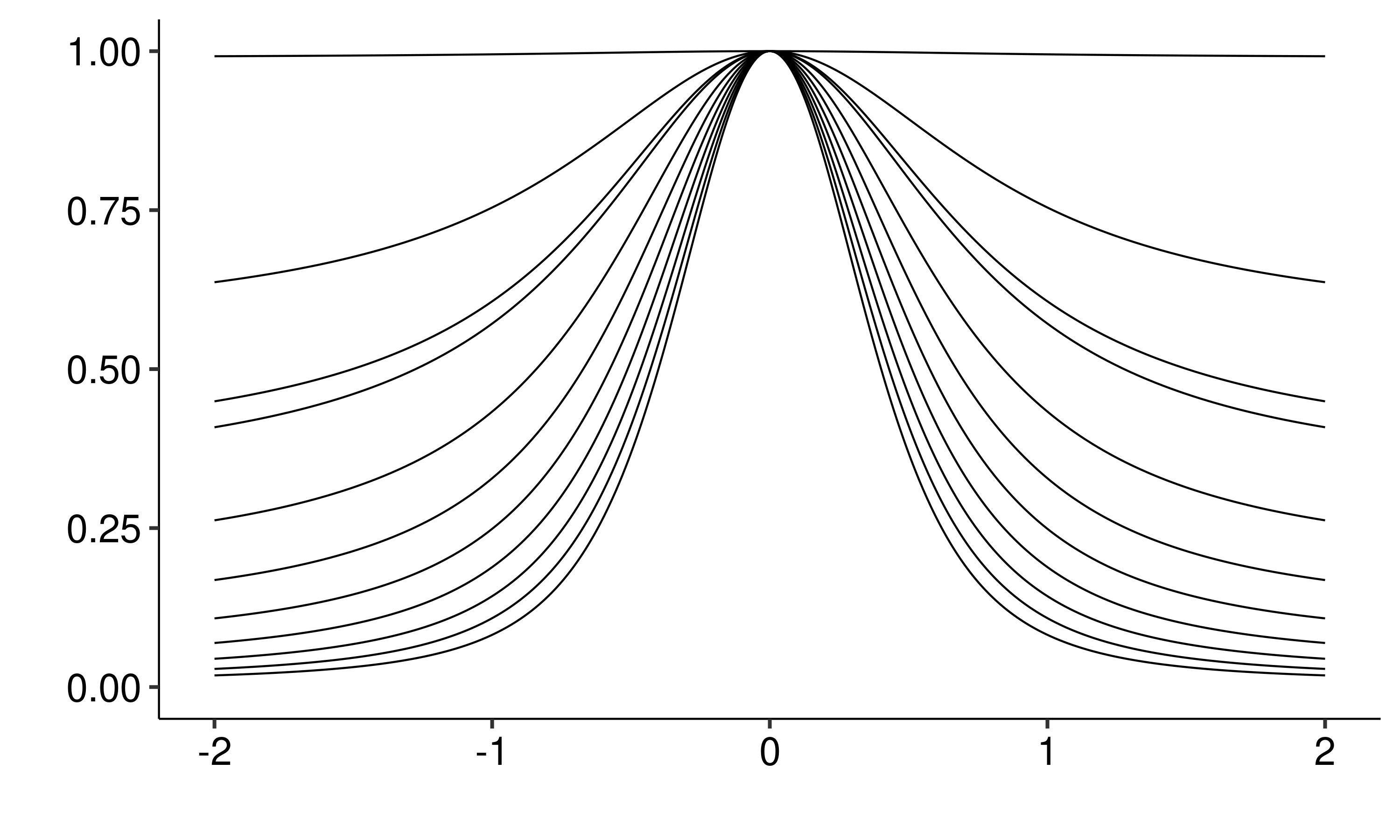
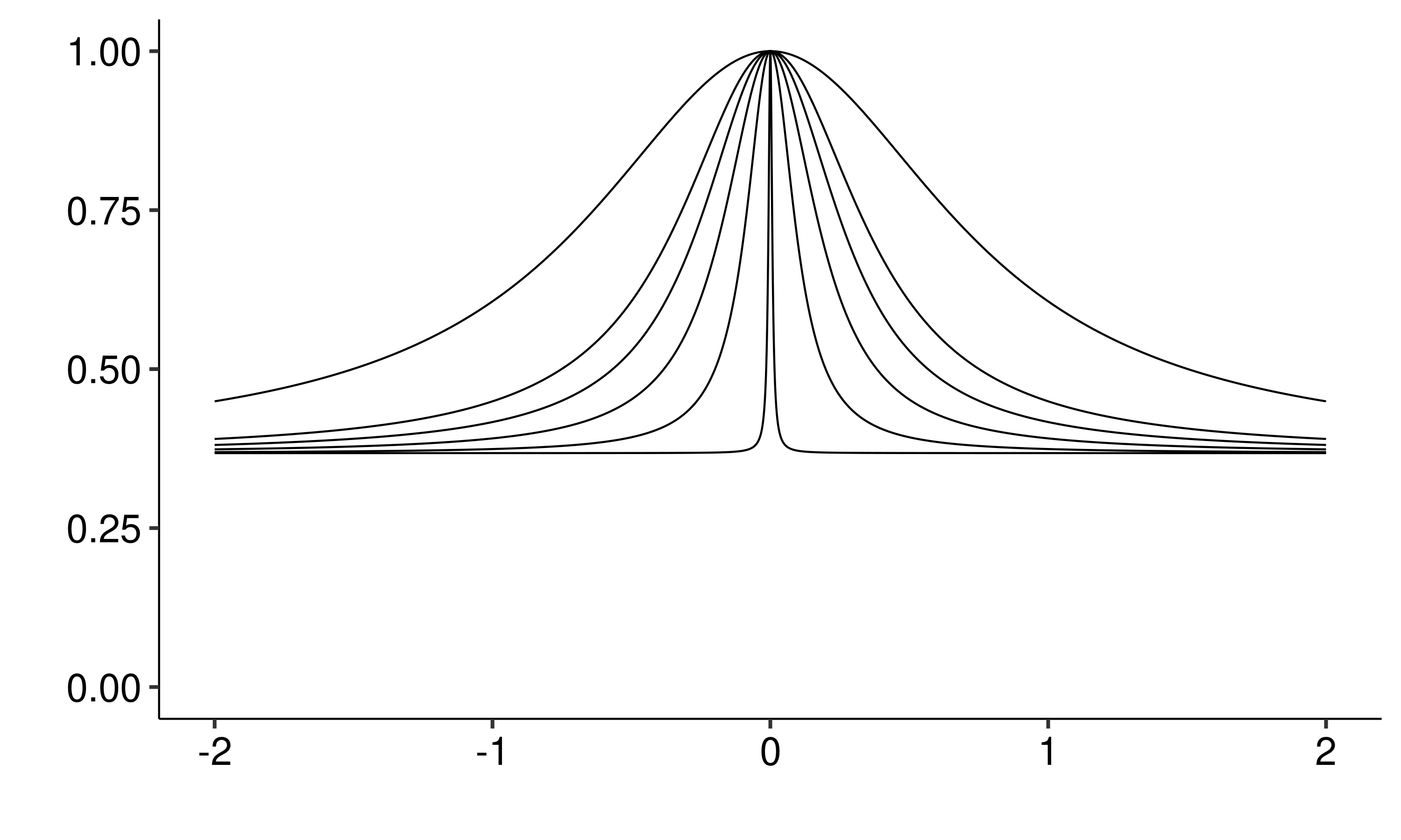
Moreover, note that for spike-and-slab regression, it is the flat part that is approximated by a distribution, not the Dirac measure. In other words, both the SIC prior and the spike-and-slab regression prior propose working with a distribution that approximates a mixture of a flat prior and a Dirac measure, but they do not approximate the same term of the mixture. In addition, Equation (13) reveals that the influence of the flat prior is determined by . In addition, the "" terms is proportional to a distribution that approximates the Dirac measure, with tuning the bias of the approximation. Figure 4 indicates how variations in or affect the prior density. Typically, a flat prior is employed to allocate substantial prior mass to large values, contrary to most prior distributions used for variable selection purposes (Gaussian, Laplace and Horseshoe priors). Then, the prior distribution (9) allows to rely on a flat prior (non-informative in some sense) for large values, and also to simultaneously promote values close to 0.
For SIC penalization, the tuning parameter is suggested to be fixed as , as proposed by O’Neill and Burke, (2023), suggesting an analogy with regularization and the BIC procedure as a rationale behind the definition of . However, according to the interpretation of the prior distribution , we suggest that could be tuned based on prior beliefs regarding the expected number of null coordinates. Thus, the default choice "" implies that confidence in potentially assigning certain coordinates to 0, is primarily driven by the amount of available data.
Asymptotic behavior. To have a better understanding of the prior, we consider the limit behaviour of when is large and/or is small. Since we deal with improper distribution, usual convergence modes cannot be used. That is why Bioche and Druilhet, (2016) proposed a convergence mode adapted to the Bayesian framework where prior distributions are defined up to a scalar factor. When the priors are Radon measures, that is distributions finite on compact sets, they derive a quotient topology called q-vague topology. A sequence converge q-vaguely to if there exists positive scalars such that converges weakly to , or equivalently, if for any real-valued continuous function with compact support, we have The q-vague limit of , when it exists, is unique up to a scalar factor. Moreover, when the likelihood is continuous, the posterior distributions also converge q-vaguely to . Proofs are detailed in Appendix A.
Proposition 3.1.
Let be a sequence that converges to . Then, for fixed, the related sequence converges q-vaguely to a Dirac measure in .
Proposition 3.2.
Let be a sequences that converge to . Then, for fixed, the related sequence converges q-vaguely to a flat prior.
We now study the convergence of when goes to and goes to simultaneously. The limit will depend on the relative rate of convergence of and . When goes to much faster than goes to , then converges to a flat prior. Similarly, when goes to much much slower than goes to then converges to the Dirac measure . To give a precise meaning of "much faster" or much slower", the following proposition give the relative rate of convergence corresponding to the phase transition, where the limit is between a flat distribution and a Dirac measure.
Proposition 3.3.
Assume that goes to and goes to with for some constant . Then, the related sequence converges q-vaguely to the prior .
3.2 Oracle inequality
The aim of this section is to demonstrate that the SIC penalty satisfies the required frequentist theoretical properties. In particular, we target to highlight that prediction error performance is similar to that of other penalization methods. The theoretical argument we obtain provides reliable guarantees for using a SIC penalization approach, akin to an oracle inequality. To achieve this, we examine squared error loss under a fixed design.
For the following theoretical results, we carry out a standard mathematical procedure used to demonstrate the oracle inequality of the LASSO (Tibshirani,, 1996). For more details, we refer the reader to Zou and Hastie, (2005); Bühlmann and Van De Geer, (2011); Hastie et al., (2015); Tibshirani and Wasserman, (2015). For what follows, assume the linear model:
To ensure that these procedures are valid within the framework of the SIC penalty, we introduce Lemma 3.4, which shows how to upper bound the SIC penalty with usual norms.
Lemma 3.4 (Links between and norms).
For a -dimensional vector, and for , we have:
| (14) |
Lemma 3.5 (Basic Inequality).
Let be a solution of (8). An optimality condition for the SIC estimator is given by
The dominant term of the inequality is random, and to ensure a non-random upper bound of the left term, the following relies on a concentration result. First, using Holder’s inequality, an upper bound on the random term is written as,
Following Bühlmann and Van De Geer, (2011) we introduce the set and choose . For a suitable value of , the set has large probability. Note by the diagonal elements of the normalized Gram matrix: , for .
Lemma 3.6.
Suppose that for , . For all , we pose ,
Corollary 3.6.1.
(Inequality of SIC consistency) Assume that for we have . For , let , where is an estimator of . Then, with a probability of at least we have
Then, denotes the support for the unknown parameter vector , in other words: the set of active variables. For any vector , the following vectors are also defined and , this means that if is in then the component of the vector is non-zero. Then, can be expressed as a function of and :
Lemma 3.7.
Assume that , and , then with large probability we have
and
By exploiting the compatibility condition related to in Bühlmann and Van De Geer, (2011), and for some , for all such that, we have
which leads to
Theorem 3.8.
Assuming the compatibility condition on , and for , we can rewrite the lemma basic inequality in the following form:
Corollary 3.8.1.
(Oracle Inequality) Assume for , and that the compatibility condition is satisfied on the set , then it exists a constant for and such that:
4 Sparse covariate estimation
In the following, we consider the context of the PLN model (1), focusing on the parameter of interest, matrix , for which we aim to achieve sparse estimation. To this end, we adopt a regularized log likelihood lower bound (2) with a SIC penalty as our loss function. This can also be viewed as a PLN model with a SIC constraint on the regression coefficients. The ELBO of the log-likelihood is an objective function widely used in the estimation of regression models when the true log-likelihood is intractable (You et al.,, 2014; Carbonetto and Stephens,, 2012; Zhang et al.,, 2019). As detailed in Section 3.2, the SIC penalty is able to constrain and capture sparse patterns in the model with guaranteed convergence to the -norm. The objective function to be optimized is then:
where denote the SIC penalty matrix which is derived as and is the number of unpenalized parameters. Here is a fixed tuning parameter which maximizes a pseudo-BIC (Chen et al.,, 2018) due to the replacement of the true log-likelihood in the SIC criterion (4) by the ELBO (2).
Optimization algorithm. To sparsly estimate the support of the entries in the regressor matrix, we combine the PLN estimation algorithm proposed by Chiquet et al., (2021) and the -telescoping algorithm proposed by O’Neill and Burke, (2023). The resulting algorithm we propose is described in Algorithm 1, and first we provide details about steps of the procedure.
-
-
The pseudo-Fisher information matrix denoted by is given from the matrix of negative second derivatives of with respect to and the pseudo penalized scoring matrix denoted by is given from the gradient of with respect to . The penalized pseudo-Fisher information matrix is:
where is the observed information of the unpenalized ELBO; and is a diagonal matrix that arises due to penalization, where each entry is given by , except for the first diagonal terms which are zero because the intercepts of the count columns are not penalized. Note that the computation of the inverse of relies on a QR decomposition (Stewart,, 1973) in order to avoid numerical problems.
-
-
The penalized scoring matrix expression is given by:
where is a matrix of row and column whose components come from .
-
-
The update of during the optimization procedure is obtained by the -telescoping approach on a penalized pseudo-Fisher scoring algorithm. In particular at te -th iteration, is updated according to: .
5 Simulation study
5.1 Setup
To evaluate the proposed approach, we perform a simulation study, on different synthetic databases and with different methods.
Compared methods. To provide a context for the performance of the proposed method compared to existing methods, we apply the following methods in this simulation study.
-
-
GLMNET: a univariate Poisson regression model using Lasso regularization (implemented in the
Rglmnetpackage). As this modeling is univariate, we duplicate it separately for each column of the count matrix . While this approach disregards the dependence between columns of , at least it includes a variable selection procedure. -
-
PLN: the standard Poisson Log Normal model implemented in the
RpackagePLNmodels. Unlike the GLMNET approach, this is a multivariate approach that takes the dependence between columns of Y into account, but it does not perform variable selection.
Simulation protocol. Below we describe how synthetic data are simulated according to PLN model (1), to assess the performance of different models in relevant configurations.
-
-
Dimensions. We consider diverse sample sizes and species numbers .
-
-
To generate the design matrix . The design matrix consists of six covariate column vectors , , , , , , where the entries of each covariate are drawn independently from a uniform distribution .
-
-
Model parameters. The coefficient matrix is the parameter of interest for the proposed approach, and in particular we choose to make this matrix sparse by setting some coefficients to zero, enabling us to assess how well the proposed method recovers coefficients that are exactly equal to zero. For coefficients different from zero, we choose to set some at 0.5 and others at 1 to assess if this induces a difference in the ability to estimate them. Concerning the covariance matrix , two scenarios are considered (and a third one is also provided with Supplementary Materials), in order to evaluate the impact on the ability to accurately estimate coefficients and effectively recover coefficients equal to zero.
-
1.
Full: indicating that the counts are dependent across species. In this case, we derive the covariance matrix by where each entry of is drawn independently from a . In this case, all entries of are non-negative.
-
2.
Diagonal: indicating that is a diagonal matrix whose the terms are different and are drawn independently from a . In this case, the species are uncorrelated from each other and they have a specific variance coefficient.
-
1.
- -
Databases are generated for all possible combinations of the following elements: sample size , number of species , and dependence structure in the matrix . The process to generate a database is repeated 100 times and the results are averaged over these 100 repetitions, in order to effectively compare the performance of different methods.
Performance indicator. Given the focus of this article, we propose evaluating the performance of the different methods on databases using three indicators, detailed in the following.
-
-
Estimation error: the relative error based on the Frobenius norm between the true value of coefficients matrix and the estimated coefficient matrix . In particular, the indicator is the same as in Wu et al., (2018), which is:
-
-
Support error: the true negative rate (TNR), which measures how coefficients equal to zero (called negative) are accurately estimated as being equal to zero (called true negative).
-
-
Prediction error: the mean square error between the true value of and .
5.2 Comparison of prediction formulas
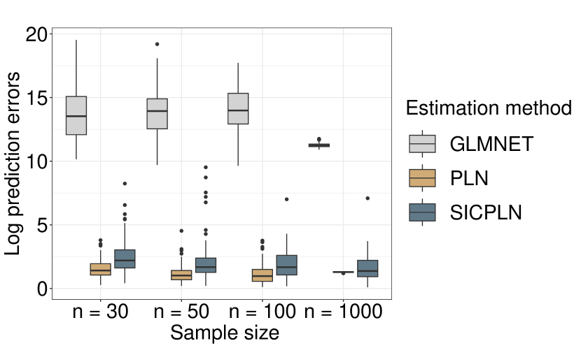
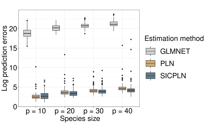
To illustrate the performance of the two prediction formulae outlined in Section 2.3, we simulate 100 datasets on which the PLN model is fitted. Specifically, each database is simulated under the scenario of a full covariance structure. The results of this simulation are presented in Figure 5, showing that the prediction formula not involving variational parameters generally yields weak results. In the following sections on the simulation study of prediction and variable selection performance, PLN performances are evaluated based on predictions made by the formula yielding the best results, which is the formula involving variational parameters.
5.3 Simulation results
Numerical results for one configuration. To straightforwardly present numerical results of competing methods, we propose highlighting the estimated coefficients of each method in the configuration where: , , and the structure of is the Full case. Table 1 provides the results of coefficients estimation. We observe that SICPLN outperforms GLMNET for accurate coefficient estimation, probably because GLMNET uses a LASSO penalty, which can introduce bias into the estimates. In addition, unlike GLMNET, SICPLN exploits dependency structures between multidimensional responses to improve estimates. Finally, with SICPLN, coefficients associated with irrelevant variables are estimated as exactly zero, which is not always the case with GLMNET (see species 4).
| Species | Estimation method | ||||||
| Species 1 | True coefficient | 0 | 1 | 1 | 1 | 1 | 0 |
| PLN | 0.08 | 1.04 | 1.09 | 1.07 | 1.10 | 0.09 | |
| GLMNET | 0 | 0.91 | 0.99 | 0.93 | 0.96 | 0 | |
| SICPLN | 0 | 0.95 | 1 | 0.98 | 0.92 | 0 | |
| Species 2 | True coefficient | 0.5 | 0 | 0 | 1 | 1 | 0 |
| PLN | 0.55 | 0.07 | 0.15 | 1.04 | 0.99 | 0.13 | |
| GLMNET | 0.43 | 0 | 0 | 0.98 | 0.87 | 0 | |
| SICPLN | 0.47 | 0 | 0 | 0.98 | 0.92 | 0 | |
| Species 3 | True coefficient | 1 | 0.5 | 0.5 | 1 | 1 | 0 |
| PLN | 1.10 | 0.58 | 0.54 | 1.05 | 1.06 | 0.10 | |
| GLMNET | 0.97 | 0.39 | 0.43 | 1.05 | 0.84 | 0 | |
| SICPLN | 1 | 0.48 | 0.44 | 0.96 | 0.97 | 0 | |
| Species 4 | True coefficient | 1 | 1 | 0 | 0 | 0.5 | 0 |
| PLN | 0.91 | 0.95 | 0.05 | 0.10 | 0.52 | 0.02 | |
| GLMNET | 0.64 | 1.14 | 0.10 | -0.14 | 0.14 | -0.21 | |
| SICPLN | 0.94 | 0.98 | 0 | 0 | 0.54 | 0 |
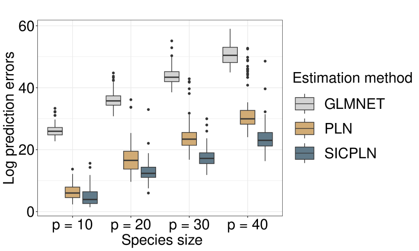
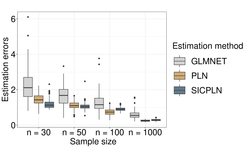
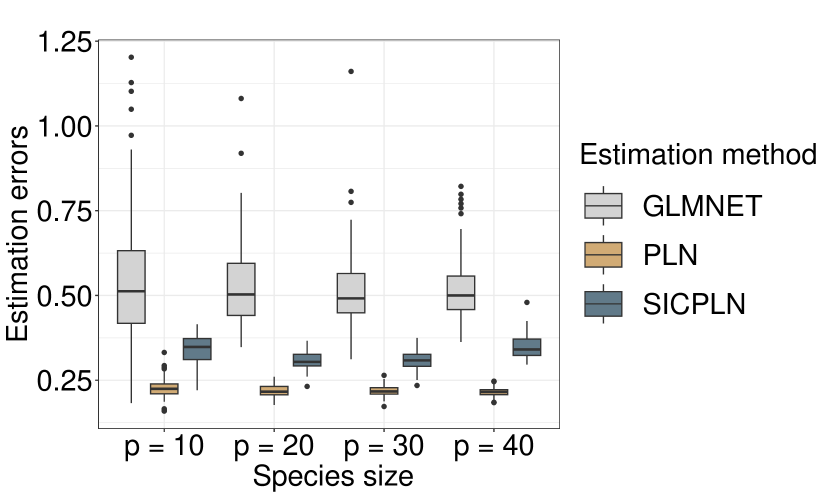
Results in terms of estimation error. Figure 6(a) shows that coefficient estimation accuracy is improved when the dependency structure between counts is taken into account. In addition, as Table 1 shows, SICPLN leads to sparser and more accurate estimates. In Figure 6(b), when the number of columns in the count matrix increases, indicating complexity in the dependency structure between counts, the estimation error with GLMNET significantly increases compared to PLN and SICPLN. The estimation errors of SICPLN also increase as the number of columns in the count matrix increases. What we observe here can be explained by two phenomena described in the following. The first one is related to the tendency of SICPLN to overly shrink or to set exactly to zero all coefficients associated with species with multiple irrelevant variables. The second one could be linked to the non-convergence of the algorithm during the Fisher scoring step. However, in the less complex situations represented in figures 8, i.e. when there is no dependency between the count columns, the estimation errors with GLMNET remain very high compared with SICPLN and PLN when the sample size becomes large and the number of columns in the count matrix increases.
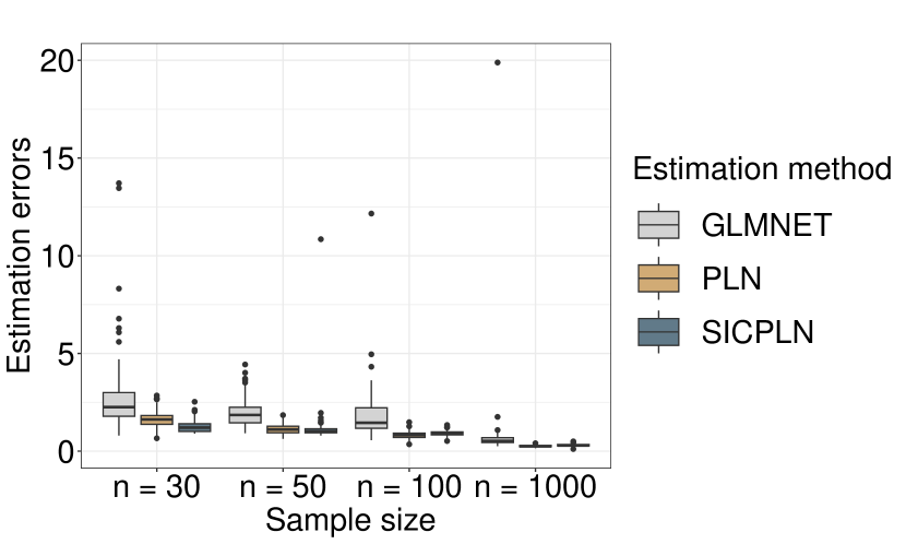
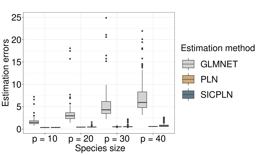
Results in terms of true negative rate. The averaged true negative rates on 100 replications are presented in Table 2 for various sample sizes. Similarly, Table 3 displays these rates for different numbers of columns in the count matrix. We observe that the true negative rates increases for each method when the sample size increases. SICPLN performs better than GLMNET in terms of sparsity measurement, showing a tendency to accurately estimate exactly zero entries in the regression coefficient matrix. The increase in the number of columns in the count matrix leads to a degradation of GLMNET and SICPLN true negative rates, especially in presence of dependencies between counts. The degradation of the average true negative rate of SICPLN is primarily due to non-convergence, resulting in coefficients that are not exactly set to zero. In the presence of a simpler dependency structure, SICPLN exhibits significantly higher true negative rates compared to GLMNET.
| Covariance structure | Sample size | GLMNET | PLN | SICPLN |
|---|---|---|---|---|
| Full | 0.006 | 0 | 0.79 | |
| Diagonal | 0.09 | 0 | 0.82 | |
| Full | 0.007 | 0 | 0.79 | |
| Diagonal | 0.08 | 0 | 0.9 | |
| Full | 0.07 | 0 | 0.87 | |
| Diagonal | 0.13 | 0 | 0.90 | |
| Full | 0.18 | 0 | 0.98 | |
| Diagonal | 0.22 | 0 | 0.95 |
| Covariance structure | Species size | GLMNET | PLN | SICPLN |
|---|---|---|---|---|
| Full | 0.01 | 0 | 0.55 | |
| Diagonal | 0.17 | 0 | 0.91 | |
| Full | 0.007 | 0 | 0.19 | |
| Diagonal | 0.11 | 0 | 0.92 | |
| Full | 0.006 | 0 | 0.04 | |
| Diagonal | 0.09 | 0 | 0.93 | |
| Full | 0.005 | 0 | 0.07 | |
| Diagonal | 0.09 | 0 | 0.90 |
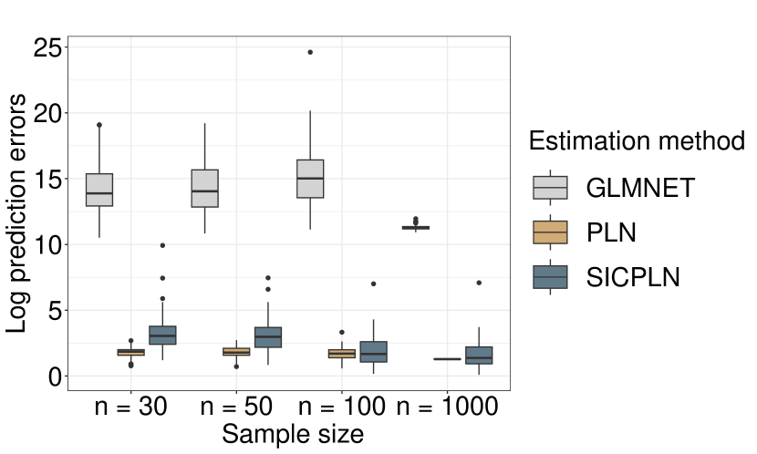
Results in terms of prediction error. Prediction errors obtained for various sample sizes and species are presented in figures 7 and 9, on 100 replications. We observe that when the sample size is small, prediction errors for PLN and SICPLN are lower compared to GLMNET. However, as the sample size increases, the performance of SICPLN improves significantly compared to PLN and GLMNET in terms of prediction accuracy. Additionally, we observe that for a fixed sample size , variations of the number of columns in the counting matrix yield better prediction performances for SICPLN compared to PLN and GLMNET when the covariance structure is in the Full case. Nonetheless, when counts are independent , SICPLN often shrinks to zero the coefficients associated with species that have multiple non-relevant variables. This leads to a slight increase in the estimation error of SICPLN coefficients compared to PLN, but the prediction errors between SICPLN and PLN remain similar.
6 Real data analyses
We illustrate the proposed method through the analysis of two real abundance datasets. Our aim is to identify the relevant environmental variables that describe or control the abundances observed in the count matrix.
6.1 Genus data
Data description. We first consider the genus data set from the R package SCGLR,
recently reanalysed by Chauvet et al., (2019).
The data set describes the abundance of 15 tree genera common to Congo Basin forests, measured on 1000 parcels.
To explain these genera, 46 environmental variables are available.
Among these, 21 variables describe the physical characteristics of the environment,
such as altitude, rainfall, soil conditions, and so on.
Vegetation properties are represented by 25 photosynthetic activity indices obtained by teledetection,
including EVI (Enhanced Vegetation Indexes), MIR (Middle InfraRed) and NIR (Near-InfraRed).
Some categorical variables such as inventory, mois_sec_50, mois_sec_100, geology
and spatial coordinates, longitude (center_x) and latitude (center_y), are also available.
A preliminary analysis examined the correlations between the variables.
This was done by calculating the variance inflation factor (VIF) for each variable.
We then grouped all vegetation indices into a new variable called vegetation_index
and aggregated all rainfall variables from pluvio_1 to pluvio_12 into a single variable called rainfall.
Based on the VIF results in Table 4, we only consider 4 variables:
vegetation_index, wetness, center_x, center_y and surface. Following the approach of Chauvet et al., (2019), we treat the variable surface as an offset variable and then apply PLN, SICPLN and GLMNET.
| Variables | vegetation index | rainfall | altitude | awd | mcwd | wetness | CWD | center x | center y | pluvio an |
|---|---|---|---|---|---|---|---|---|---|---|
| VIF | 1.92 | 14588.77 | 7.27 | 42.28 | 43.17 | 2.02 | 29.40 | 10.89 | 21.77 | 14690.40 |
| Variables | vegetation index | wetness | center x | center y |
|---|---|---|---|---|
| VIF | 1.36 | 1.75 | 1.46 | 1.51 |
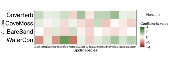
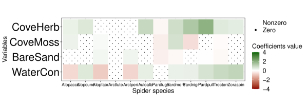
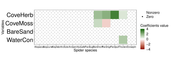
Results. The estimated coefficients for each species are shown in Figure 10. This figure first includes the results obtained with the simple PLN model (Figure 10(a)). Next, Figure 10(b) shows the coefficients obtained with GLMNET, where the abundance of each species is modeled in a univariate way (without taking into account the dependency structure) using a LASSO-based penalized Poisson regression. Finally, Figure 10(c) shows the results obtained with the SICPLN approach.
The regression coefficients estimated by the PLN model are non-zero,
posing challenges in identifying relevant explanatory variables that significantly influence the abundance of species.
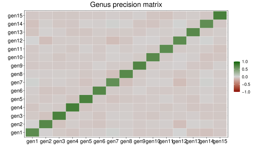
The estimates derived from GLMNET are close to those obtained with SICPLN in terms of sparsity.
This closeness is certainly due to the lack of dependence between the genus species, as illustrated in
Figure 14(a).
Specifically, 16 out of 60 coefficients were estimated as non-zero with GLMNET, compared to only 8 out of 60 for SICPLN.
The abundance of most species does not seem to be related to environmental variables.
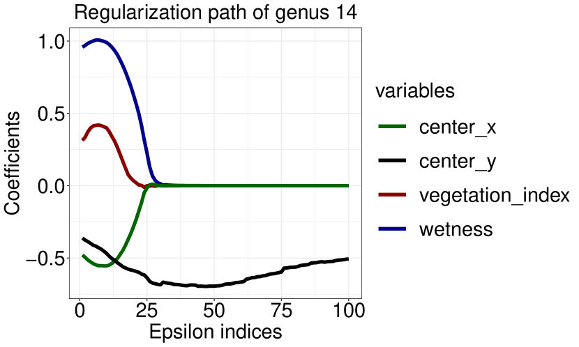
Only the abundance of genus 8, genus 9, genus 12, genus 13, and genus 14
appears to be explained by one or more environmental variables.
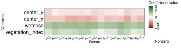
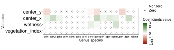
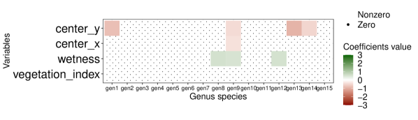
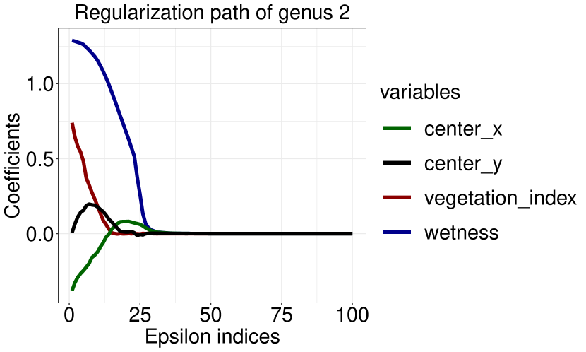
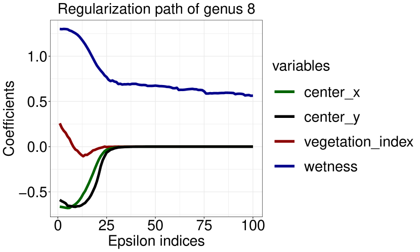
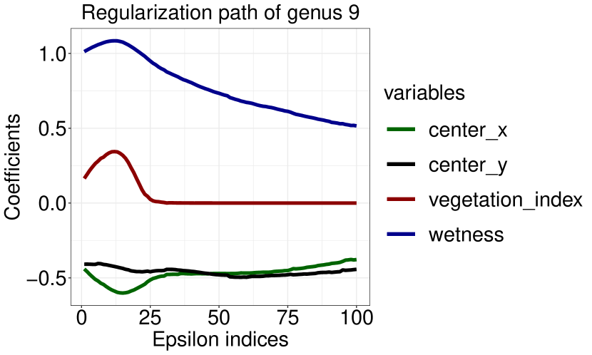
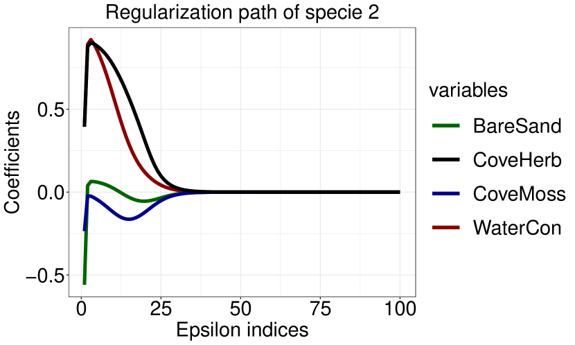
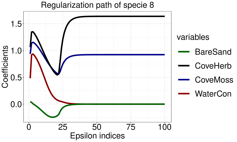
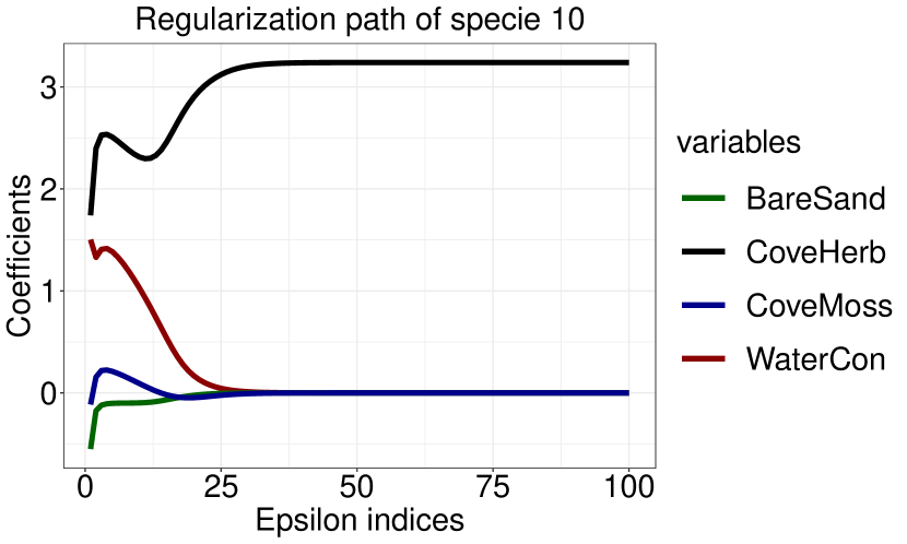
Figure 11
shows the regularization path using the SIC criterion.
Unlike the LASSO (Tibshirani,, 1996) or elastic net (Zou and Hastie,, 2005) regularization path,
it does not show the evolution of the coefficient values
as a function of parameter driving the intensity of regularization.
Instead, it shows the evolution of the estimated coefficients during the optimization step using the telescoping approach,
which aims to move the problem closer to the penalty.
This eventually sets the coefficient of the irrelevant variables to zero
and stabilizes the coefficient of the relevant variables at a non-zero value.
It is worth noting that relevant variables may vary from one species to another.
For instance, no variable is selected for genus 2
(Figure 11(a)),
only wetness is selected for genus 8
(Figure 11(b)),
and variables wetness, center_x and center_y are selected for genus 9
(Figure 11(c)).
6.2 The hunting spider dataset
Data description.
The hunting spider dataset used in this study, initially introduced by Smeenk-Enserink and Van der Aart, (1974),
comes from the R package VGAM.
These data give the abundance of 12 spider species captured in traps across 28 sites.
To characterize the observed abundances, six environmental variables are considered, namely
WaterCon (log percentage of soil dry mass), BareSand (log percentage cover of bare sand),
FallTwig (log percentage cover of fallen leaves and twigs), CoveMoss (log percentage cover of the moss layer),
CoveHerb (log percentage cover of the herb layer), and
ReflLux (Reflection of the soil surface with cloudless sky).
| Variables | WaterCon | BareSand | FallTwig | CoveMoss | CoveHerb | ReflLux |
| VIF | 4.34 | 2.28 | 5.87 | 2.67 | 2.48 | 6.04 |
Results.
After performing the VIF analysis (see Table 6),
we selected the variables with a VIF coefficient lower than .
These variables include WaterCon, BareSand, CoveMossand CoveHerb.
Figure 12 shows that
the estimated coefficients with PLN are all non-zero, while
those obtained with GLMNET (univariate Poisson regression) contained non-zero coefficients out of .
Conversely, our approach SICPLN provides the sparsest coefficients, with only non-zero coefficients out of .
The better performance of SICPLN compared to GLMNET in terms of sparsity
is due to the existence of dependencies between species
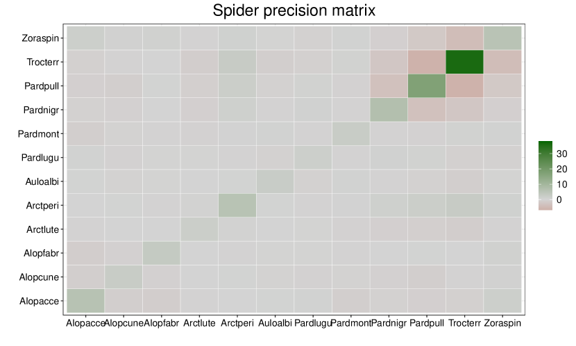
(see Figure 14(b) for the precision matrix),
which are taken into account by SICPLN but not by GLMNET.
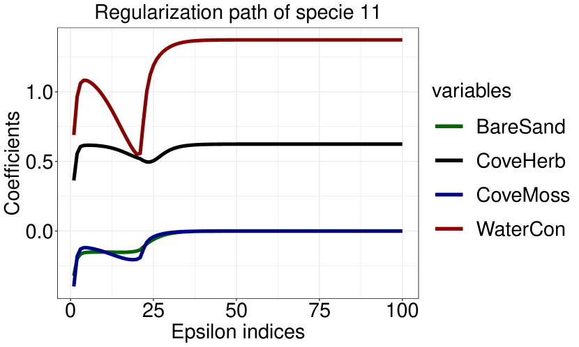
Figure 13
shows the SICPLN regularization path used to select the most relevant variables
to explain the abundance of four spider species.
These results highlight that variables CoveHerb and CoveMoss is selected for species 8 (Pardmont),
variables CoveHerb and WaterCon is selected to explain the abundance of specie 11 (Trocterr),
while only CoveHerb are selected for specie 10 (pardpull).
No variable is considered relevant to explain the abundance of specie 2 (Alopcune).
7 Discussion
In this article, we present a method for variable selection in a PLN model, providing both theoretical and practical assurances regarding its effective application. In particular, a classical frequentist theoretical analysis is given by presenting an oracle inequality, highlighting the asymptotic behavior as the sample size increases. Concerning the proposed implementation, the estimation procedure involves an algorithm (-telescoping) that we combine with the PLN fitting procedure, and that progressively reduces to 0, aiming to closely approximate the -penalty and thereby achieve good variable selection performance. To the best of our knowledge, it is not entirely clear theoretically what ensures variable selection as tends to 0. One would expect to obtain a theoretical result indicating that variable selection performance increases as approaches 0. To begin addressing this issue, we present first results regarding this penalization approach, from a Bayesian analysis point of view. The results does not fully elucidate what happens as tends to 0 since the prior distribution should be defined based on a fixed in a Bayesian framework and cannot evolve, as the -telescoping algorithm does in the frequentist approach O’Neill and Burke, (2023). Nevertheless, in the case of a straightforward transposition of this penalization approach into a Bayesian model, Proposition 3.2 shows that if is too close to 0, then the prior distribution reduces to a flat prior. However, when studying the prior distribution behavior with regards to the joint evolution of and , with Proposition 3.3, we observe a convergence rate at which the prior distribution converges to a mixture of a Dirac measure and a flat prior. Although this result corresponds to a very specific case, it demonstrates a first connection between the reduction of towards 0 and a Bayesian mechanism of variable selection. In practice, from Section 5, we observe that the proposed procedure yields results with comparable performance to PLN, and even outperforms it. Additionally, the resulting inference provides sparse estimates, which are highly beneficial in real-world contexts, as demonstrated in Section 6.
Following the work in this article, a potential future work may involve implementing this penalization method in the case of a zero-inflated PLN model, which can cover a broader range of database configurations requiring such modeling. In the same vein, it could be possible to extend this penalization method to the precision matrix as well, with the hope of improving estimation performance. Next, another research initiative involves developing an approach for a modification of cross-validation based on robust predictions of new data. From the results presented above, we find that prediction errors using formula "PLN prediction" in Section 2.3, are too high to ensure proper tuning parameter calibration via cross-validation. Additionally, using formula "Variational PLN prediction" in cross-validation would require obtaining variational parameters related to validation data. However, these variational parameters, for the -th individual, depend, among other, on count data . Therefore, it’s not possible to obtain these variational parameters if the -th data point is not in the training sample. Furthermore, based on our current investigations, inferring these variational parameters from the variational parameters estimated on the training sample is not feasible, as they exhibit significant variation depending on the count data .
References
- Aitchison and Ho, (1989) Aitchison, J. and Ho, C. (1989). The multivariate poisson-log normal distribution. Biometrika, 76(4):643–653.
- Akaike, (1974) Akaike, H. (1974). A new look at the statistical model identification. IEEE transactions on automatic control, 19(6):716–723.
- Bioche and Druilhet, (2016) Bioche, C. and Druilhet, P. (2016). Approximation of improper priors. Bernoulli, 22(3):1709–1728.
- Blei et al., (2017) Blei, D. M., Kucukelbir, A., and McAuliffe, J. D. (2017). Variational inference: A review for statisticians. Journal of the American statistical Association, 112(518):859–877.
- Bühlmann and Van De Geer, (2011) Bühlmann, P. and Van De Geer, S. (2011). Statistics for high-dimensional data: methods, theory and applications. Springer Science & Business Media.
- Carbonetto and Stephens, (2012) Carbonetto, P. and Stephens, M. (2012). Scalable Variational Inference for Bayesian Variable Selection in Regression, and Its Accuracy in Genetic Association Studies. Bayesian Analysis, 7(1):73 – 108.
- Chauvet et al., (2019) Chauvet, J., Trottier, C., and Bry, X. (2019). Component-based regularization of multivariate generalized linear mixed models. Journal of Computational and Graphical Statistics, 28(4):909–920.
- Chen and Chen, (2008) Chen, J. and Chen, Z. (2008). Extended bayesian information criteria for model selection with large model spaces. Biometrika, 95(3):759–771.
- Chen et al., (2018) Chen, Y.-C., Wang, Y. S., and Erosheva, E. A. (2018). On the use of bootstrap with variational inference: Theory, interpretation, and a two-sample test example. The Annals of Applied Statistics, 12(2):846 – 876.
- Chib and Winkelmann, (2001) Chib, S. and Winkelmann, R. (2001). Markov chain monte carlo analysis of correlated count data. Journal of Business & Economic Statistics, 19(4):428–435.
- Chiquet et al., (2018) Chiquet, J., Mariadassou, M., and Robin, S. (2018). Variational inference for probabilistic poisson pca. The Annals of Applied Statistics, 12(4):2674–2698.
- Chiquet et al., (2021) Chiquet, J., Mariadassou, M., and Robin, S. (2021). The poisson-lognormal model as a versatile framework for the joint analysis of species abundances. Frontiers in Ecology and Evolution, 9:588292.
- Chiquet et al., (2019) Chiquet, J., Robin, S., and Mariadassou, M. (2019). Variational inference for sparse network reconstruction from count data. In International Conference on Machine Learning, pages 1162–1171. PMLR.
- Choi et al., (2017) Choi, Y., Coram, M., Peng, J., and Tang, H. (2017). A poisson log-normal model for constructing gene covariation network using rna-seq data. Journal of Computational Biology, 24(7):721–731.
- Fan and Li, (2001) Fan, J. and Li, R. (2001). Variable selection via nonconcave penalized likelihood and its oracle properties. Journal of the American statistical Association, 96(456):1348–1360.
- Grollemund et al., (2023) Grollemund, P.-M., Lenoir, L., Benoit, J., Chassard, C., and Bord, C. (2023). Permanova testing and poisson log-normal modelling unravel how two traditional cheeses are distinguished through sorting and verbalization tasks. Food Quality and Preference, 104:104732.
- Hall et al., (2011) Hall, P., Ormerod, J. T., and Wand, M. P. (2011). Theory of gaussian variational approximation for a poisson mixed model. Statistica Sinica, pages 369–389.
- Hastie et al., (2015) Hastie, T., Tibshirani, R., and Wainwright, M. (2015). Statistical learning with sparsity: the lasso and generalizations. CRC press.
- Heinze et al., (2018) Heinze, G., Wallisch, C., and Dunkler, D. (2018). Variable selection–a review and recommendations for the practicing statistician. Biometrical journal, 60(3):431–449.
- Ishwaran and Rao, (2005) Ishwaran, H. and Rao, J. S. (2005). Spike and slab variable selection: frequentist and Bayesian strategies. Ann. Statist., 33(2):730–773.
- Karlis and Xekalaki, (2005) Karlis, D. and Xekalaki, E. (2005). Mixed poisson distributions. International Statistical Review/Revue Internationale de Statistique, pages 35–58.
- Mitchell and Beauchamp, (1988) Mitchell, T. J. and Beauchamp, J. J. (1988). Bayesian variable selection in linear regression. J. Amer. Statist. Assoc., 83(404):1023–1036. With comments by James Berger and C. L. Mallows and with a reply by the authors.
- Nikoloulopoulos and Karlis, (2009) Nikoloulopoulos, A. K. and Karlis, D. (2009). Modeling multivariate count data using copulas. Communications in Statistics-Simulation and Computation, 39(1):172–187.
- O’Neill and Burke, (2023) O’Neill, M. and Burke, K. (2023). Variable selection using a smooth information criterion for distributional regression models. Statistics and Computing, 33(3):71.
- Park and Lord, (2007) Park, E. S. and Lord, D. (2007). Multivariate poisson-lognormal models for jointly modeling crash frequency by severity. Transportation Research Record, 2019(1):1–6.
- Park and Casella, (2008) Park, T. and Casella, G. (2008). The bayesian lasso. Journal of the American Statistical Association, 103(482):681–686.
- Rothman et al., (2010) Rothman, A. J., Levina, E., and Zhu, J. (2010). Sparse multivariate regression with covariance estimation. Journal of Computational and Graphical Statistics, 19(4):947–962.
- Schwarz, (1978) Schwarz, G. (1978). Estimating the dimension of a model. The annals of statistics, pages 461–464.
- Shi and Valdez, (2014) Shi, P. and Valdez, E. A. (2014). Multivariate negative binomial models for insurance claim counts. Insurance: Mathematics and Economics, 55:18–29.
- Smeenk-Enserink and Van der Aart, (1974) Smeenk-Enserink, N. and Van der Aart, P. (1974). Correlations between distributions of hunting spiders (lycosidae, ctenidae) and environmental characteristics in a dune area. Netherlands Journal of Zoology, 25(1):1–45.
- Sohn and Kim, (2012) Sohn, K.-A. and Kim, S. (2012). Joint estimation of structured sparsity and output structure in multiple-output regression via inverse-covariance regularization. In Artificial Intelligence and Statistics, pages 1081–1089. PMLR.
- Stewart, (1973) Stewart, G. W. (1973). Introduction to matrix computations. Elsevier.
- Stoehr and Robin, (2024) Stoehr, J. and Robin, S. S. (2024). Composite likelihood inference for the poisson log-normal model. arXiv preprint arXiv:2402.14390.
- Thierry et al., (2023) Thierry, A., Madec, M.-N., Grondin, C., Rué, O., Mariadassou, M., and Valence, F. (2023). Microbial communities of a variety of 75 homemade fermented vegetables. Frontiers in Microbiology, 14:1323424.
- Tibshirani, (1996) Tibshirani, R. (1996). Regression shrinkage and selection via the lasso. Journal of the Royal Statistical Society: Series B (Methodological), 58(1):267–288.
- Tibshirani and Wasserman, (2015) Tibshirani, R. and Wasserman, L. (2015). Sparsity and the lasso. Statistical machine learning, pages 1–15.
- Tzikas et al., (2008) Tzikas, D. G., Likas, A. C., and Galatsanos, N. P. (2008). The variational approximation for bayesian inference. IEEE Signal Processing Magazine, 25(6):131–146.
- Wu et al., (2018) Wu, H., Deng, X., and Ramakrishnan, N. (2018). Sparse estimation of multivariate poisson log-normal models from count data. Statistical Analysis and Data Mining: The ASA Data Science Journal, 11(2):66–77.
- You et al., (2014) You, C., Ormerod, J. T., and Mueller, S. (2014). On variational bayes estimation and variational information criteria for linear regression models. Australian & New Zealand Journal of Statistics, 56(1):73–87.
- Zhang et al., (2019) Zhang, C.-X., Xu, S., and Zhang, J.-S. (2019). A novel variational bayesian method for variable selection in logistic regression models. Computational Statistics & Data Analysis, 133:1–19.
- Zhang et al., (2017) Zhang, Y., Zhou, H., Zhou, J., and Sun, W. (2017). Regression models for multivariate count data. Journal of Computational and Graphical Statistics, 26(1):1–13.
- Zou, (2006) Zou, H. (2006). The adaptive lasso and its oracle properties. Journal of the American statistical association, 101(476):1418–1429.
- Zou and Hastie, (2005) Zou, H. and Hastie, T. (2005). Regularization and variable selection via the elastic net. Journal of the Royal Statistical Society Series B: Statistical Methodology, 67(2):301–320.
Appendix A Proofs and mathematical details
About the geometry of SIC
Consider here the case of a 2-dimensional balls related to the SIC function , so that results correspond to Figure 1. The contours of the balls associated with a value are defined by the following constraint: and by using that the reciprocal expression of given by: , it follows the result that:
Proof of Proposition 3.1
When goes to , converges to by applying the monotone convergence theorem. This means that the weight of the flat part in the prior goes to . Let be a continuous real-valued function with compact support and , we have from (13)
Since is bounded with compact support, the first part converges to . Since converges narrowly to , the second part converges to . Therefore, converges q-vaguely to a flat prior. Therefore, converges q-vaguely to a Dirac measure in .
Proof of Proposition 3.2
Put . When converge to , converges to and therefore converge to . We have
Since is bounded and is a probability distribution, the second part goes to . The first part is the integral of w.r.t. the flat prior . Therefore, converges q-vaguely to a flat prior.
Proof of Proposition 3.3
Denote .
Part 1 : we prove that
We have
Now, we show that the second integral converge to . Note that for , we have and then, with ,
Nxt, we show that the first integral converge to . For we have . Therefore, we can apply the dominated convergence theorem:
Part 2 : we prove that converge narrowly to the Dirac measure . It is sufficient to prove that, for any , when . Similarly to Part 1, after the same change of variables, we have :
For , we have . Then
Part 3: let be a continuous real-valued function with compact support and . From (13):
The result follows.
Proof of Lemma 3.4
First inequality. Since we have
which implies that .
Second inequality. Consider the target inequality: for a value , which does not depend on . Then, notice that this inequality holds if for each coordinate , and if :
Consider the function , for , for which the first derivative is . It is straightforward to see that for all , , and then the result follows with .
Third inequality. Note that we can write , where and are -dimensional vectors, those the elements are and , if . In the case of , then and . First, consider the -dimensional vector those the element is and remark that , and that . Second, note that . Then, using the Cauchy-Schwarz inequality, we have that:
Proof of Basic Inequality 3.5
By definition of from Equation (8), we have the following inequality:
| (15) |
Rearranging and by substituting gives
and we finally have
Proof of Lemma 3.6
Posing , . We know that , then and are:
By Gaussian concentration inequality we know that if , then for all ,
applying this to yields to
Then, we can derive the following inequality:
For we obtain for each :
Proof of Corollary 3.6.1
Using Basic Inequality 3.5, for , with a probability of at least we have:
To prove the large probability at least we use
thus
Moreover, by choosing , we have
Proof of Lemma 3.7
Proof of Theorem 3.8
Proof of Oracle Inequality 3.8.1
From
we can write
for , and
By posing we find