Multiple Chern bands in twisted MoTe₂ and possible non-Abelian states

Abstract

We investigate the moiré band structures and possible even denominator fractional quantum Hall state in small angle twisted bilayer MoTe₂, using combined large-scale local basis density functional theory calculation and continuum model exact diagonalization. Via large-scale first principles calculations at $\theta=1.89^{\circ}$, we find a sequence of $C=1$ moiré Chern bands, in analogy to Landau levels. Constructing the continuum model with multiple Chern bands and uniform Berry curvature in the second moiré band, we undertake band-projected exact diagonalization using unscreened Coulomb repulsion to pinpoint possible $\nu=-3/2$ non-Abelian states across a wide range of twist angles below $\theta=2.5^{\circ}$.

Moiré materials based on transition metal dichalcogenides (TMDs) have emerged as a promising domain for exploring novel quantum phenomena [1, 2]. Owning to the substantial effective mass inherent to TMDs valence bands and the persistence of narrow moiré bands across various twist angles, these materials showcase a diverse array of correlated electron states, characterized by pronounced interaction effects, including Mott and charge-transfer insulators[3, 4, 5, 6, 7, 8, 9, 10], generalized Wigner crystals [5, 11, 12, 13, 14, 15, 16, 17], and quantum anomalous Hall (QAH) effect [18]. Remarkably, recent transport experiments on twisted MoTe₂ have provided unambiguous evidences of both integer and odd-denominator fractional quantum anomalous Hall (QAH and FQAH) effects[19, 20], and the signature for fractional quantum spin Hall effect at hole filling factor $\nu=-3$ [21]. The observations of FQAH were made within a range of fairly large twist angles, specifically $\theta\sim 2.7^{\circ}-3.9^{\circ}$, evidenced through both optical [22] and compressibility [23] measurements, within the first moiré valence band. While the recent experiment on fractional quantum spin Hall (FQSH) effect [21] at small angle $\theta\sim 2.1^{\circ}$ revealed the remarkable triple quantum spin Hall effects, driving the interest to higher filling factors and small twisted angles.

The realization of fractional quantum anomalous Hall effect not only fundamentally broadens the spectrum of topological phases of matter but also holds promising prospects for harnessing the power of anyons in topological quantum computations at zero magnetic field [24, 25, 26, 27, 28]. On the theory side, the fractional Chern insulator (FCI) phases in topological flat band systems has been proposed for over a decade [29, 30, 31, 32, 32]. In recent years, within the graphene [33, 34, 35, 36] and TMD [37, 38]-based moiré system, theoretical predictions have pointed to such an exotic state at partial filling of the topological moiré flat band at long moiré wavelength. Non-Abelian quantum Hall states such as the possible Moore-Read state [39] at even-denominator filling factor $\nu=5/2$ has been discussed in Landau level [40]. Under particle-hole symmetry breaking [41, 42] (e.g. Landau level mixing or local three-body interaction), several numerical studies [43, 44, 45, 46] have shown that the Moore-Read Pfaffian (anti-Pfaffian) state with six-fold ground state degeneracies may be favored. Early numerical studies proposed that topological flat band models may host a fermionic non-Abelian Moore-Read state under synthetic three-body interaction [47] or long range dipolar interaction [48]. However, a realistic simulation of such a non-Abelian state in a microscopic lattice model remains challenging. Recent experiment on fractional quantum spin Hall effect [21] indicates the possibility of a time-reversal pair of the even-denominator $3/2$ FQAH states, reveals a strong candidate for the emergence of a non-Abelian state of topological moiré minibands in twisted MoTe₂. Motivated by these developments, we theoretically analyze and propose the realistic conditions for the emergence.

In this work, we start from the local basis first-principle calculations and continuum model at $\theta=1.89^{\circ}$, and study the possible non-Abelian state at $\nu=-3/2$, filled to the second moiré valence band. From local basis density functional calculations (DFT), we find the number of $C=1$ Chern bands increases from 2 [49, 50] to 5 when twist angle changes from $\theta=5.08^{\circ}$ to $\theta=1.89^{\circ}$. The Chern number of DFT bands are directly calculated from Berry curvature and Wilson loop from DFT wave functions. Moreover, we confirm the multiple $C=1$ bands from edge states calculations.

For the fitting the continuum model at $\theta=1.89^{\circ}$, we constrain the parameter space via fixing the Chern number of top five valence bands and increasing the weight of second moiré bands. With the small angle continuum model, we find strong evidences for the Moore-Read states through momentum-space exact diagonalization spectrum in several different lattice geometries. The ground state degeneracy and momentum locations fulfill the generalized Pauli principle[51, 52] for Moore-Read state  [39] for even and odd number of electrons, similar to those in the half-filled first excited Landau level. Our study provides a detailed study of multiple topological bands in twisted MoTe₂ and the continuum model for realizing non-Abelian states, paving the way for its materials realizations.

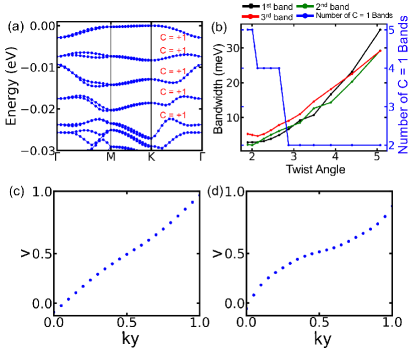
Figure 1: (a) Band structures for homobilayer MoTe₂ with twist angle 1.89^∘, where the five flat bands near the Fermi level possess a Chern number of $C=1$. (b) Angle dependent band width and number of $C=1$ bands 1.89^∘ to 5.08^∘, calculated by local-basis DFT. The black, green, and red dotted lines denote for the band width of the first, second, and third band. The blue dotted line represent for the number of C = 1 bands. The evolution of Wannier charge center for the (c) first band and (d) second band, indicating that C = 1.

DFT results for twist angle $\theta=1.89^{\circ}$. Here we employ the local-basis OpenMX package, utilizing Projected Atomic Orbitals (PAOs) specified as Mo7.0-s3p2d1 and Te7.0-s3p2d2 [53, 54]. The real-space Hamiltonian is determined by the hopping strength between different sites, while the overlap parameters are calculated using the PAOs as follows:

$$H_{i\alpha,j\beta}=\sum_{n}\left\langle\phi_{i\alpha}\left(\mathbf{r}-\tau_{i}\right)|\hat{H}|\phi_{j\beta}\left(\mathbf{r}-\tau_{j}-\mathbf{R}_{n}\right)\right\rangle$$ (1)

$$S_{i\alpha,j\beta}=\sum_{n}\left\langle\phi_{i\alpha}\left(\mathbf{r}-\tau_{i}\right)\mid\phi_{j\beta}\left(\mathbf{r}-\tau_{j}-\mathbf{R}_{n}\right)\right\rangle$$

where i, j, $\alpha$, and $\beta$ represent atom and orbital indices, $\tau_{j}$ and $R_{n}$ denote for the atomic and lattice position. Then, the eigenvalues $E_{n\gamma}$ and eigen-vectors $v_{n\gamma,j\beta}$ can be determined by the generalized eigenvalue problem:

$$\sum_{j\beta}\left(H_{i\alpha,j\beta}-E_{n\gamma}S_{i\alpha,j\beta}\right)v_{n\gamma,j\beta}=0$$ (2)

For simplicity, we rewrite the eigen-vectors $v_{n\gamma,j\beta}$ as $\left|v_{n}(\mathbf{k})\right\rangle$. The PBE exchange-correlation functional and the norm-conserving pseudopotential [55] are employed in the calculation with single $\Gamma$ $k$-sampling, and we set the convergence criterion as $6\times 10^{-5}$ Hartree. For the twist angle of 1.89^∘, there are 1838 Mo atoms and 3676 Te atoms, forming a Hamiltonian with 191152 dimensions [56]. Since full diagonalization of such a Hamiltonian is unrealistic in present hardware platform, we apply the shift-and-invert trick, recasting the generalized eigenvalues problem to the eigenvalues problem, and then apply the Lanczos algorithm to get part of the eigenvalues near Fermi level as commonly used in linear-scaling DFT [57, 58].

In twisted MoTe₂, the twist angle emerges as a degree of freedom for manipulating the electronic structures. As shown in Fig. 1, our DFT calculations demonstrate a clear trend: a decrease in the twist angle leads to a reduction in the bandwidth near the Fermi level. For a relatively large twist angle of 5.08^∘, the smallest bandwidth is 29 meV for the second band, consistent with plane-wave DFT [50, 56]. However, at the small twist angle of 1.89^∘, five nearly flat bands emerge near the Fermi level, with a small bandwidth of 2.9, 2.2, 5.3, 3.7, and 4.6 meV, respectively. As a result of $C_{2y}$ symmetries, bands along the $\Gamma K$ lines are doubly degenerate, while a clear splitting is observed along the $\Gamma M$ line as shown in Fig. 1(a). Furthermore, our results show multiple band inversions near a twist angle of 1.89^∘, leading to the formation of topological flat bands. These bands are distinctively separated from others by a band gap ranging from 1.9 meV to 3.9 meV. The band separation hints at the possibility of various QSH states [21], including single, double, triple QSH states, with increased hole doping in the system.

With twisted Hamiltonian, we then proceed to study the topological properties of narrow bandwidth moiré valence band. We note the previous $C_{3}$ symmetry indicator at $C_{3z}$ symmetric momenta can not accurately determine the Chern numbers with modulo three [37]. The precise calculation requires the momentum space integration of Berry curvature or Berry connection. Despite Kramer pairs have a Chern number of zero due to time-reversal symmetry, a significant Berry curvature can still manifest within a single valley. To separate the single valley from the Hamiltonian, we construct the valley operator $\hat{s}_{z}$ based on the atomic positions and orbital elements, and separate the single-valley eigen-vectors $\left|u_{m}(\mathbf{k})\right\rangle$ from the entire eigen-vectors $\left|v_{m}(\mathbf{k})\right\rangle$ based on the expectation value of $\hat{s}_{z}$:

$$S_{mn}^{z}(\mathbf{k})=\left\langle u_{m}(\mathbf{k})|\hat{s}_{z}|u_{n}(\mathbf{k})\right\rangle$$ (3)

Across the two-dimensional Brillouin zone, most of the lines—excluding the $\Gamma K$ and $MK$ lines—are non-degenerate, with their expectation values of $\hat{s}_{z}$ approaching either $+1$ or $-1$. For those lines that are degenerate, a basis transformation is implemented to construct the disentangled wavefunctions, characterized by expectation values of $+1$ or $-1$. This allows us to feasibly separate the single-valley eigenvectors from the valley-mixed eigenvectors.

Therefore, the valley Chern number can be calculated by the integral of the Berry curvature for the single-valley eigen-vectors. Due to the large number of atomic orbitals, the Kubo formula approach requiring full diagonalization is inapplicable here. Therefore, we calculate the Berry curvature distribution $F(\mathbf{k})$ through the Fukui-Hatsugai-Suzuki method [59]:

$$U_{\Delta\mathbf{k}}(\mathbf{k})=\operatorname{det}\left\langle u_{n}(\mathbf{k})\mid u_{m}(\mathbf{k}+\Delta\mathbf{k})\right\rangle$$ (4)

$$F(\mathbf{k})=\operatorname{Im}\log U_{\Delta k_{1}}(\mathbf{k})U_{\Delta k_{2}}\left(\mathbf{k}+\Delta k_{1}\right)\times$$

$$U_{\Delta k_{1}}^{-1}\left(\mathbf{k}+\Delta k_{2}\right)U_{\Delta k_{2}}^{-1}(\mathbf{k}),$$

where $U_{\Delta k_{1}}(\mathbf{k})$ is the overlap matrix between two neighboring wave vectors, and $u_{n}(\mathbf{k})$ denote for the single-valley wave function for the nth band. By integrating the Berry curvature over the entire Brillouin zone, the Chern number for a single band can be determined by the formula: $C_{n}=\frac{1}{2\pi}\int F(\mathbf{k})dk^{2}$. As shown in Fig. 2(a), the distribution of Berry curvature is not uniform across the Brillouin zone, highlighting significant topological interest. To further verify the nontrivial characteristics, we also examine the evolution of Wannier charge centers [60, 61]:

$$\nu_{n}(k_{y})=\int\left\langle u_{n}(\mathbf{k})\left|\partial_{k_{x}}\right|u_{n}(\mathbf{k})\right\rangle dk_{x}$$ (5)

As illustrated in Fig. 1(c) and  1(d), the number of crossings between the WCC and any horizontal lines is 1, indicating the Chern number of 1. Furthermore, $C=1$ for top five moiré bands will lead to the presence of multiple pairs of gapless edge states inside bulk gap. This is clearly illustrated in Fig. S1(b), thereby confirming the topological properties of the flat Chern bands.

Continuum model with high harmonic term. To perform the many-body calculation, we start with the continuum model for twisted MoTe₂ [62]. Here we incorporate the higher-order harmonic terms for both inter-layer and intra-layer coupling, extending up to the second harmonics. Considering the significant momentum difference between the two valleys ($1/a\gg 1/a_{m}$), we ignore the inter-valley coupling, focusing solely on the K valley. Additionally, we limit our model to single-spin, owning to the large Ising spin-orbit coupling in MoTe₂. As a result, we arrive at the following continuum model for the K valley:

$$\hat{H_{s}}=\begin{bmatrix}-\frac{\bm{(\hat{k}-K_{t})^{2}}}{2m^{*}}+\Delta_{t}(\bm{r})&\Delta_{T}(\bm{r})\\ \Delta^{\dagger}_{T}(\bm{r})&-\frac{\bm{(\hat{k}-K_{b})^{2}}}{2m^{*}}+\Delta_{b}(\bm{r})\end{bmatrix}$$ (6)

with:

$$\Delta_{l}(\bm{r}) =2V_{1}\sum_{i=1,3,5}\cos(\bm{g^{1}_{i}\cdot r}+l\phi_{1})+2V_{2}\sum_{i=1,3,5}\cos(\bm{g^{2}_{i}\cdot r})$$ (7)

$$\Delta_{T} =w_{1}\sum_{i=1,2,3}e^{-i\bm{q^{1}_{i}\cdot r}}+w_{2}\sum_{i=1,2,3}e^{-i\bm{q^{2}_{i}\cdot r}}$$

where $\bm{\hat{k}}$ is the momentum, $\bm{K_{t}}(\bm{K_{b}})$ is high symmetry momentum $\bm{K}$ of the top(bottom) layer, $\Delta_{t}(\bm{r})(\Delta_{b}(\bm{r}))$ is the layer dependent moiré potential, $l=+1$ for top layer and $l=-1$ for bottom layer; $\Delta_{T}(\bm{r})$ is the interlayer tunneling, $\bm{G_{i}}$ is moiré reciprocal vector, $\bm{g_{i}^{1}}$ and $\bm{g_{i}^{2}}$ represent the momentum differences between the nearest and second-nearest plane wave bases within the same layer. Similarly, $\bm{q_{i}^{1}}$ and $\bm{q_{i}^{2}}$ denote the momentum differences between the nearest and second-nearest plane wave bases across different layers.

Figure 2: The Berry curvature distributions across the two-dimensional Brillouin zone for the second band, calculated by (a) first-principles calculations and (b) continuum model. We note the distribution is similarly positive and uniform, and sums to a Chern number of 1.

To derive the parameters of continuum model, we adopt two guiding principles in the fitting of DFT band structures. Firstly, we ensure that the Chern numbers for top five valence bands are equal to 1, close related to Landau levels [63]. Subsequently, particular focus is placed on the second band, for which we minimize the error of band dispersion and Berry curvature distribution as much as possible. From our DFT calculation at $\theta=1.89^{\circ}$, we obtain the parameters as:

$$\phi_{1}=-90.0^{\circ},V_{1}=2.4\ meV,V_{2}=1.0\ meV$$ (8)

$$w_{1}=-5.8\ meV,w_{2}=2.8\ meV$$

The fitting results are shown in Fig. S1(a), where the major topological features are captured in the continuum model. Figure  2(b) displays the distributions of Berry curvature, where both the shape and magnitude closely resemble those obtained from DFT calculations. Additionally, the new parameters effectively capture the variation in the Chern number with the twist angle, as demonstrated in Fig 4.(b), where the top three bands consistently exhibit $C=1$ within the range of $1^{\circ}$ to $3^{\circ}$. It is found that the potential terms are significantly smaller than those derived from the DFT bands at larger twist angle $\theta>2.89^{\circ}$ [50, 56, 64, 65]. This difference indicates that the parameters previously employed do not effectively describe the higher moiré valence bands at small twist angles ($\leq 2.5^{\circ}$).

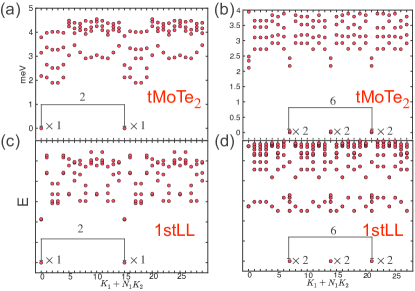
Figure 3: Exact diagonalization spectrum. (a)/(b) The many-body spectrum from the ED calculation on the 30(28) sites cluster at filling factor $\nu=-\frac{3}{2}$ with the continuum model of MoTe₂ at $\theta=2.0^{\circ}$ and we use the dielectric constant $\epsilon=5$. (c)/(d) The same calculation on the 1st Landau Level, which agrees well with our results from continuum model.

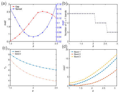
Figure 4: (a) The red dot denotes the band gap from the ED spectrum, which is defined as the energy difference between the quasi-degenerate states and the excited states. Besides, the blue dot is used to represent the energy spread between the quasi-degenerate ground states. Both data are derived from our ED calculation performed on the 28 sites cluster. (b) The number of bands which have chern number $C=1$ in the top five moiré bands from the continuum model, it agrees well with the local basis DFT results as we show in Fig.1(b) between 1${}^{\circ}\sim 3^{\circ}$. (c) The fluctuation of Berry curvature of the top two band in the continuum model. (d) The bandwidth of top three moiré bands from the continuum model.

Exact Diagonalization at $\nu=-3/2$. With the continuum model tailored for $\theta=1.89^{\circ}$ and multiple Chern bands, we project the interaction on the second moiré bands, and start with the spontaneous spin polarized assumption to reduce the Hilbert space dimension, which is consistent with large anomalous Hall resistance at small angle devices for filling factor $1\leq\nu\leq 2$ [21]. The complete many-body Hamiltonian is then expressed as:

$$H =H_{s}+V,$$ (9)

$$V =\sum_{s,s^{\prime}}\frac{1}{2}\int\int d\bm{r_{1}}d\bm{r_{2}}V(\bm{r_{1}-r_{2}})\hat{c}_{s}^{\dagger}(\bm{r_{1}})\hat{c}_{s^{\prime}}^{\dagger}(\bm{r_{2}})c_{s^{\prime}}(\bm{r_{2}})c_{s}(\bm{r_{1}})$$

Here, $H_{s}$ is the single particle continuum model Hamiltonian of hole and V is the Coulomb interaction, $c^{\dagger}_{s}(\bm{r})$ is the creation operator of hole in real space ,s is the spin index and we use long range Coulomb interaction:$V(\bm{r_{1}-r_{2}})=\frac{e^{2}}{\epsilon|\bm{r_{1}}-\bm{r_{2}}|}$ and choose the realistic dielectric constant $\epsilon=5$. We then project the model Hamiltonian into the second moiré valence bands:

$$H_{s}=\sum_{nks}\epsilon_{nks}a^{\dagger}_{nks}a_{nks},$$ (10)

$$V=\frac{1}{2}\sum_{\bm{n}\bm{s}\bm{k}}V_{n_{1}k_{1}n_{2}k_{2}n_{3}k_{3}n_{4}k_{4}}^{s_{1}s_{2}s_{3}s_{4}}\hat{a}^{\dagger}_{n_{1}k_{1}s_{1}}\hat{a}^{\dagger}_{n_{2}k_{2}s_{2}}\hat{a}_{n_{3}k_{3}s_{3}}\hat{a}_{n_{4}k_{4}s_{4}},$$

$$V_{n_{1}k_{1}n_{2}k_{2}n_{3}k_{3}n_{4}k_{4}}^{s_{1}s_{2}s_{3}s_{4}}=\int\int d\bm{r_{1}}d\bm{r_{2}}V(\bm{r_{1}-r_{2}})\times$$

$$\psi^{*}_{n_{1}k_{1}s_{1}}(\bm{r_{1}})\psi^{*}_{n_{2}k_{2}s_{2}}(\bm{r_{2}})\psi_{n_{3}k_{3}s_{3}}(\bm{r_{2}})\psi_{n_{4}k_{4}s_{4}}(\bm{r_{1}})$$

where n is the band index, $a^{\dagger}_{nks}$ is the creation operator of Bloch states, $\psi_{nks}$ is the eigen-vector of continuum model, $\hat{c}^{\dagger}_{s}(\bm{r})=\sum_{nks}\psi^{*}_{nks}(\bm{r})\hat{a}^{\dagger}_{nks}$, $\sum_{\bm{n}}=\sum_{n_{1}n_{2}n_{3}n_{4}}$ and so on.

Our calculations focus on the filling $\nu=-3/2$ of single valley for twist angles within the range $\theta\in[1.5^{\circ},2.5^{\circ}]$, which encompasses experimental twist angles [21]. Our primary findings are depicted in Fig. 3, revealing several quasi-degenerate ground states. Specifically, we identify two-fold quasi-degenerate states for the 30-site cluster (15 electrons),and six-fold degenerate states for the 28-site cluster (14 electrons). Both the momentum location and ground state degeneracy agree well with the requirement of the generalized Pauli principle, where no more than two particles in four consecutive orbitals, called (2,2)-admissible “root” configuration[51, 52] . In short, for an odd number of electrons, the possible (2,2)-admissible“root” configuration [66] requires that only the occupation partition “$1010\cdots 101010$” and its translational invariant partner“$0101\cdots 010101$” are allowed, explaining the two-fold degeneracy. But for even number of electrons, there are six possible configurations, which explain the six-fold degeneracy as demonstrated in the Supplemental Material. The different degeneracies observed for odd and even number of electrons provide compelling evidence suggesting that the ground states may be the Non-Abelian Moore-Read states.

We then perform the twist angle dependent exact diagonalizations. Our analysis reveals that the energy spread between degenerate states reaches a minimum around 2^∘, while the global gap peaks around 2.2^∘, as depicted in Figure 4(a). This observation suggests that the system may offer optimal conditions for potential Non-Abelian states at approximately 2^∘. Moreover, we perform a comparative examination of the states within twisted MoTe₂ and the 1st Landau Level (1st LL), uncovering notable parallels, as depicted in Fig. 3. Additionally, we extend our calculations to clusters of varying sizes, with detailed methodologies outlined in the Supplemental Material. Together, these findings underscore the remarkable similarity to the 1st LL across different system configurations.

Given the preservation of particle-hole symmetry in dispersionless Landau levels, the ground states are expected to be symmetrized Moore-Read states, comprising superpositions of Pfaffian and anti-Pfaffian states, owing to potential finite size effects [43, 67, 68]. However, the missing of particle-hole symmetry in our moiré band-projected Hamiltonian would restrict the non-Abelian nature of the ground states at $\nu=-3/2$. Consequently, further investigation is warranted to elucidate the precise nature of the topological order in this context.

Conclusion and outlook. In this study, we investigate the single-particle electronic structures of small-angle moiré MoTe₂ with local basis DFT, exploring its topological properties through Berry curvature and Wilson loop calculations. Specifically, we concentrate on the second moiré band, constructing a continuum model comprising up to five $C=1$ Chern bands. This model offers insight into various charge fractionalization phenomena reminiscent of those observed in Landau level systems.

Drawing an analogy to the first excited Landau level, our exact diagonalization reveals a remarkably similar many-body spectrum for $\nu=-3/2$ in both even and odd electron systems, providing compelling evidences for the existence of non-Abelian states. We note that in realistic situations, breaking the particle-hole symmetry will lead to the favored Moore-Read Pfaffian. Numerically, the Pfaffian or antiPfaffian nature of the ground states may be distinguished by adding opposite three body interactions, or density-matrix renormalization group calculation of their entanglement spectrum, originating from the different edge structures.

The discovery of integer and fractional quantum Hall effects in the moiré MoTe₂ [19, 20] and pentalayer graphene [69] at zero magnetic field provides ideal material platforms for the realization of charge fractionalization beyond the conventional two-dimensional electron gas at high magnetic field. Similar to a partially filled Landau level, a partially filled topological band can exhibit a symphony of distinct phases as a function of filling factor, each bringing its own novelty as an impetus to extend the frontier of condensed matter physics. While earlier investigations primarily centered on first Chern bands, our study broadens this focus to higher moiré bands, uncovering a series of $C=1$ bands, laying the foundation for the study of higher filling factor fractional states [21].

Note: Near the completion of this work, we became aware of a related work [70], which studied the non-Abelian state using Skyrmion model and its application in twisted semiconductor bilayers.

Appendix

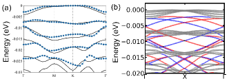
Figure S1: (a) The comparative analysis of the band structures for twist angle 1.89^∘. Blue points/lines illustrated the results from OpenMX calculations, while the black line represents the fitting results from continuum model. (b) Band structure of twisted MoTe₂ nanoribbon, calculated from OpenMX hamiltonian. The trivial bulk states are shown in gray, while spin-up/-down edge states are in red/blue.

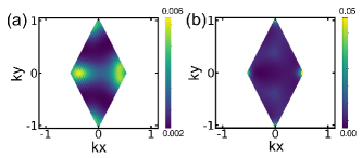
s

Figure S2: The DFT Berry curvature distributions of $\theta=1.89^{\circ}$ for the (a) top valence band and (b) second valece band.

.1 Lattice relaxation for homobilayer MoTe₂ with twist angle $1.89^{\circ}$

To relax the structure, we utilize the ab initio deep potential (DP) molecular dynamics method. Our methodology begin with constructing $3\times 3\times 1$ MM, MX, and XM configurations and 28 distinct intermediate transition states [71]. Each configurations are relaxed at a fixed volume and then subjected to 200 random perturbations. We then gather initial data sets through 20 fs ab initio molecular dynamics simulations, calculating energies, forces, and virial tensors using VASP. This data set is used to train the DP model, utilizing a descriptor (DeepPot-SE) for both angular and radial atomic configurations and embedding layers mapping descriptors to atomic energies. Following initial training, the model undergoes molecular dynamics simulations across various pressures and temperatures, generating trajectories categorized based on model deviation. Selected configurations undergo self-consistent density functional theory calculations for further training iterations. Furthermore, we expanded our training data with large-angle twisted structures and applied transfer learning principles. By freezing embedding layer parameters and focusing on the hidden and output layers, we construct the transform learning neural network that can be used to relax the homobilayer MoTe₂ with twist angle 1.89^∘.

Details about openMX calculations. Our openMX basis are Projected Atomic Orbitals (PAOs) specified as Mo7.0-s3p2d1 and Te7.0-s3p2d2 [53, 54]. The notation 7.0 indicates a cutoff radius of 7.0 Bohr. For Mo7.0-s3p2d1, s3p2d1 denotes the inclusion of 3 sets of $s$-orbitals, 2 sets of $p$-orbitals, and 1 set of $d$-orbitals, totaling 14 atomic orbitals. Similarly, Te7.0-s3p2d2 includes 3 sets of $s$-orbitals, 2 sets of $p$-orbitals, and 2 sets of $d$-orbitals, amounting to 19 atomic orbitals. These configurations are used to perform the self-consistent calculations.

.2 Chern number of top two band

Figure. S2(a) and  S2(b) presents the distributions of Berry curvature. The Chern numbers, derived from the integral of Berry curvature, are calculated to be 1 for both the first and second bands. Additionally, gapless edge states are observed within the gaps between the first and second bands, as well as between the second and third bands. This phenomenon is explicitly depicted in Fig. S1(b), thereby affirming the nature of multiple Chern numbers within separate valleys.

.3 The momentum geometry

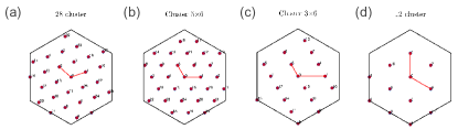
Figure S3: The Finite-sized clusters we used in the ED calculations.

We perform the ED calculation on the finite momentum cluster, which can be expressed with $\bm{k}=n_{1}\bm{t}_{1}+n_{2}\bm{t}_{2}$, and $n_{1},n_{2}$ are integers. Different geometries yield different values for $\bm{t_{1}}$ and $\bm{t_{2}}$. In this study, we utilize two unnormal momentum cluster geometries:$\bm{t}_{1}=(\bm{G}_{m1}+2\bm{G}_{m2})/6$, $\bm{t}_{2}=(\bm{G}_{m1}-\bm{G}_{m2})/6$ (Fig. S3(a))and $\bm{t}_{1}=(3\bm{G}_{m1}+\bm{G}_{m2})/14$, $\bm{t}_{2}=(-\bm{G}_{m1}+2\bm{G}_{m2})/14$ (Fig. S3(b)) and two other normal cluster geometry which we show in Fig. S3.

.4 Other ED spectrum

In this part, we show the ED results on the 12-sites and 3x6 sites cluster, which displays two-fold quasi-degenerate states for the 12-site cluster (6 electrons) and six-fold degenerate states for 3x6 cluster (9 electron). Both the momentum and degeneracy agree with the predictions of the generalized Pauli principle. And it also reveals remarkable similarities with the 1stLL, as illustrated in Fig. S4.

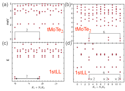
Figure S4: Exact diagnoalization spectrum. (a)/(b): the many-body spectrum from the ED calculation on the 18(12) cluster at filling factor $\nu=-\frac{3}{2}$ with the continuum model of MoTe₂ at $\theta=2.0^{\circ}$ and we use the dielectric constant $\epsilon=5$. And we use periodic condition for the 18 site cluster and anti-periodic condition for 12 site cluster. (c)/(d):the same calculation on the 1st Landau Level, which agrees well with our results from continuum model.

.5 The momentum counting from generalize Pauli principle

With the generalized Pauli principle for Moore-Read states, which means there is no more than two electron in four consecutive orbits, we calculate the momentum and degeneracy for the 28 sites and 30 sites cluster as we show in Fig. S5 and Fig. S6. For 30 sites, only the occupation partition “$1010\cdots 101010$” and its translational invariant partner“$0101\cdots 010101$” are allowed. And it also give the momentum 0 and 15 which agrees with our numerical results. With 28 sites, there are six possibilities denoted as $\Psi_{gs_{1}}$ through $\Psi_{gs_{6}}$. Additionally, the calculation of the total momentum yields three pairs of states, each with a two-fold degeneracy, all of which match our exact diagonalization results.

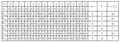
Figure S5: The counting that obeys the (2,4) admissible rule for 28 sites cluster as we show in Fig. S5.

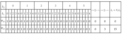
Figure S6: The counting that obeys the (2,4) admissible rule for 30 sites cluster as we show in Fig. S3(b).

References

- Kennes et al. [2021] D. M. Kennes, M. Claassen, L. Xian, A. Georges, A. J. Millis, J. Hone, C. R. Dean, D. Basov, A. N. Pasupathy, and A. Rubio, Nat. Phys. 17, 155 (2021).
- Mak and Shan [2022] K. F. Mak and J. Shan, Nature Nanotechnology 17, 686 (2022).
- Wu et al. [2018] F. Wu, T. Lovorn, E. Tutuc, and A. H. MacDonald, Phys. Rev. Lett. 121, 026402 (2018), URL https://link.aps.org/doi/10.1103/PhysRevLett.121.026402.
- Zhang et al. [2020a] Y. Zhang, N. F. Q. Yuan, and L. Fu, Phys. Rev. B 102, 201115 (2020a), URL https://link.aps.org/doi/10.1103/PhysRevB.102.201115.
- Regan et al. [2020] E. C. Regan, D. Wang, C. Jin, M. I. Bakti Utama, B. Gao, X. Wei, S. Zhao, W. Zhao, Z. Zhang, K. Yumigeta, et al., Nature 579, 359 (2020), URL https://www.nature.com/articles/s41586-020-2092-4.
- Tang et al. [2020] Y. Tang, L. Li, T. Li, Y. Xu, S. Liu, K. Barmak, K. Watanabe, T. Taniguchi, A. H. MacDonald, J. Shan, et al., Nature 579, 353 (2020), URL https://www.nature.com/articles/s41586-020-2085-3.
- Wang et al. [2020] L. Wang, E.-M. Shih, A. Ghiotto, L. Xian, D. A. Rhodes, C. Tan, M. Claassen, D. M. Kennes, Y. Bai, B. Kim, et al., Nature materials 19, 861 (2020).
- Ghiotto et al. [2021] A. Ghiotto, E.-M. Shih, G. S. Pereira, D. A. Rhodes, B. Kim, J. Zang, A. J. Millis, K. Watanabe, T. Taniguchi, J. C. Hone, et al., Nature 597, 345 (2021).
- Li et al. [2021a] T. Li, S. Jiang, L. Li, Y. Zhang, K. Kang, J. Zhu, K. Watanabe, T. Taniguchi, D. Chowdhury, L. Fu, et al., Nature 597, 350 (2021a), URL https://www.nature.com/articles/s41586-021-03853-0.
- Xu et al. [2022] Y. Xu, K. Kang, K. Watanabe, T. Taniguchi, K. F. Mak, and J. Shan (2022), URL https://arxiv.org/abs/2202.02055.
- Xu et al. [2020] Y. Xu, S. Liu, D. A. Rhodes, K. Watanabe, T. Taniguchi, J. Hone, V. Elser, K. F. Mak, and J. Shan, Nature 587, 214 (2020), URL https://www.nature.com/articles/s41586-020-2868-6.
- Zhou et al. [2021] Y. Zhou, J. Sung, E. Brutschea, I. Esterlis, Y. Wang, G. Scuri, R. J. Gelly, H. Heo, T. Taniguchi, K. Watanabe, et al., Nature 595, 48 (2021), URL https://www.nature.com/articles/s41586-021-03560-w.
- Jin et al. [2021] C. Jin, Z. Tao, T. Li, Y. Xu, Y. Tang, J. Zhu, S. Liu, K. Watanabe, T. Taniguchi, J. C. Hone, et al., Nature Materials 20, 940 (2021), URL https://www.nature.com/articles/s41563-021-00959-8.
- Li et al. [2021b] H. Li, S. Li, E. C. Regan, D. Wang, W. Zhao, S. Kahn, K. Yumigeta, M. Blei, T. Taniguchi, K. Watanabe, et al., Nature 597, 650 (2021b), URL https://www.nature.com/articles/s41586-021-03874-9.
- Huang et al. [2021] X. Huang, T. Wang, S. Miao, C. Wang, Z. Li, Z. Lian, T. Taniguchi, K. Watanabe, S. Okamoto, D. Xiao, et al., Nature Physics 17, 715 (2021), URL https://www.nature.com/articles/s41567-021-01171-w.
- Padhi et al. [2021] B. Padhi, R. Chitra, and P. W. Phillips, Physical Review B 103, 125146 (2021).
- Matty and Kim [2022] M. Matty and E.-A. Kim, Nature Communications 13, 7098 (2022).
- Li et al. [2021c] T. Li, S. Jiang, B. Shen, Y. Zhang, L. Li, Z. Tao, T. Devakul, K. Watanabe, T. Taniguchi, L. Fu, et al., Nature 600, 641 (2021c), URL https://www.nature.com/articles/s41586-021-04171-1.
- Park et al. [2023] H. Park, J. Cai, E. Anderson, Y. Zhang, J. Zhu, X. Liu, C. Wang, W. Holtzmann, C. Hu, Z. Liu, et al., Nature 622, 74 (2023).
- Xu et al. [2023] F. Xu, Z. Sun, T. Jia, C. Liu, C. Xu, C. Li, Y. Gu, K. Watanabe, T. Taniguchi, B. Tong, et al., Physical Review X 13, 031037 (2023).
- Kang et al. [2024] K. Kang, B. Shen, Y. Qiu, Y. Zeng, Z. Xia, K. Watanabe, T. Taniguchi, J. Shan, and K. F. Mak, Nature pp. 1–5 (2024).
- Cai et al. [2023] J. Cai, E. Anderson, C. Wang, X. Zhang, X. Liu, W. Holtzmann, Y. Zhang, F. Fan, T. Taniguchi, K. Watanabe, et al., Nature pp. 1–3 (2023).
- Zeng et al. [2023] Y. Zeng, Z. Xia, K. Kang, J. Zhu, P. Knüppel, C. Vaswani, K. Watanabe, T. Taniguchi, K. F. Mak, and J. Shan, Nature pp. 1–2 (2023).
- Parameswaran et al. [2013] S. A. Parameswaran, R. Roy, and S. L. Sondhi, C. R. Phys. 14, 816 (2013).
- Bergholtz and Liu [2013] E. J. Bergholtz and Z. Liu, Int. J. Mod. Phys. B 27, 1330017 (2013).
- Neupert et al. [2015] T. Neupert, C. Chamon, T. Iadecola, L. H. Santos, and C. Mudry, Phys. Scr. 2015, 014005 (2015).
- Liu and Bergholtz [2023] Z. Liu and E. J. Bergholtz, in Reference Module in Materials Science and Materials Engineering (Elsevier, 2023), p. B9780323908009001360, ISBN 978-0-12-803581-8, URL https://linkinghub.elsevier.com/retrieve/pii/B9780323908009001360.
- Nayak et al. [2008] C. Nayak, S. H. Simon, A. Stern, M. Freedman, and S. Das Sarma, Rev. Mod. Phys. 80, 1083 (2008), URL https://link.aps.org/doi/10.1103/RevModPhys.80.1083.
- Tang et al. [2011] E. Tang, J.-W. Mei, and X.-G. Wen, Phys. Rev. Lett. 106, 236802 (2011), URL https://link.aps.org/doi/10.1103/PhysRevLett.106.236802.
- Sheng et al. [2011] D. Sheng, Z.-C. Gu, K. Sun, and L. Sheng, Nat. Commun. 2, 389 (2011).
- Regnault and Bernevig [2011] N. Regnault and B. A. Bernevig, Physical Review X 1, 021014 (2011).
- Sun et al. [2011] K. Sun, Z. Gu, H. Katsura, and S. D. Sarma, Physical review letters 106, 236803 (2011).
- Repellin and Senthil [2020] C. Repellin and T. Senthil, Physical Review Research 2, 023238 (2020).
- Ledwith et al. [2020] P. J. Ledwith, G. Tarnopolsky, E. Khalaf, and A. Vishwanath, Physical Review Research 2, 023237 (2020).
- Wilhelm et al. [2021] P. Wilhelm, T. C. Lang, and A. M. Läuchli, Physical Review B 103, 125406 (2021).
- Parker et al. [2021] D. Parker, P. Ledwith, E. Khalaf, T. Soejima, J. Hauschild, Y. Xie, A. Pierce, M. P. Zaletel, A. Yacoby, and A. Vishwanath, arXiv preprint arXiv:2112.13837 (2021).
- Devakul et al. [2021] T. Devakul, V. Crépel, Y. Zhang, and L. Fu, Nature communications 12, 1 (2021), URL https://www.nature.com/articles/s41467-021-27042-9.
- Li et al. [2021d] H. Li, U. Kumar, K. Sun, and S.-Z. Lin, Phys. Rev. Res. 3, L032070 (2021d).
- Moore and Read [1991] G. Moore and N. Read, Nuclear Physics B 360, 362 (1991), ISSN 0550-3213, URL https://www.sciencedirect.com/science/article/pii/055032139190407O.
- Willett et al. [1987] R. Willett, J. P. Eisenstein, H. L. Störmer, D. C. Tsui, A. C. Gossard, and J. H. English, Phys. Rev. Lett. 59, 1776 (1987), URL https://link.aps.org/doi/10.1103/PhysRevLett.59.1776.
- Levin et al. [2007] M. Levin, B. I. Halperin, and B. Rosenow, Phys. Rev. Lett. 99, 236806 (2007), URL https://link.aps.org/doi/10.1103/PhysRevLett.99.236806.
- Lee et al. [2007] S.-S. Lee, S. Ryu, C. Nayak, and M. P. A. Fisher, Phys. Rev. Lett. 99, 236807 (2007), URL https://link.aps.org/doi/10.1103/PhysRevLett.99.236807.
- Peterson et al. [2008] M. R. Peterson, T. Jolicoeur, and S. Das Sarma, Phys. Rev. Lett. 101, 016807 (2008), URL https://link.aps.org/doi/10.1103/PhysRevLett.101.016807.
- Storni et al. [2010] M. Storni, R. H. Morf, and S. Das Sarma, Phys. Rev. Lett. 104, 076803 (2010), URL https://link.aps.org/doi/10.1103/PhysRevLett.104.076803.
- Rezayi and Simon [2011] E. H. Rezayi and S. H. Simon, Phys. Rev. Lett. 106, 116801 (2011), URL https://link.aps.org/doi/10.1103/PhysRevLett.106.116801.
- Pakrouski et al. [2015] K. Pakrouski, M. R. Peterson, T. Jolicoeur, V. W. Scarola, C. Nayak, and M. Troyer, Phys. Rev. X 5, 021004 (2015), URL https://link.aps.org/doi/10.1103/PhysRevX.5.021004.
- Bernevig and Regnault [2012a] B. A. Bernevig and N. Regnault, Phys. Rev. B 85, 075128 (2012a), URL https://link.aps.org/doi/10.1103/PhysRevB.85.075128.
- Wang et al. [2015] D. Wang, Z. Liu, W.-M. Liu, J. Cao, and H. Fan, Phys. Rev. B 91, 125138 (2015), URL https://link.aps.org/doi/10.1103/PhysRevB.91.125138.
- Reddy et al. [2023] A. P. Reddy, F. Alsallom, Y. Zhang, T. Devakul, and L. Fu, Physical Review B 108, 085117 (2023).
- Xu et al. [2024] C. Xu, J. Li, Y. Xu, Z. Bi, and Y. Zhang, Proceedings of the National Academy of Sciences 121, e2316749121 (2024).
- Haldane [1991] F. D. M. Haldane, Physical Review Letters 67, 937 (1991).
- Bernevig and Regnault [2012b] B. A. Bernevig and N. Regnault, Physical Review B 85, 075128 (2012b).
- Ozaki and Kino [2004] T. Ozaki and H. Kino, Phys. Rev. B 69, 195113 (2004).
- Ozaki [2003] T. Ozaki, Phys. Rev. B 67, 155108 (2003).
- Morrison et al. [1993] I. Morrison, D. M. Bylander, and L. Kleinman, Phys. Rev. B 47, 6728 (1993).
- Mao et al. [2023] N. Mao, C. Xu, J. Li, T. Bao, P. Liu, Y. Xu, C. Felser, L. Fu, and Y. Zhang, arXiv preprint arXiv:2311.07533 (2023).
- Bowler and Miyazaki [2012] D. R. Bowler and T. Miyazaki, Reports on Progress in Physics 75, 036503 (2012).
- Zhang et al. [2020b] Y. Zhang, H. Isobe, and L. Fu, arXiv preprint arXiv:2005.04238 (2020b).
- Fukui et al. [2005] T. Fukui, Y. Hatsugai, and H. Suzuki, Journal of the Physical Society of Japan 74, 1674 (2005).
- Yu et al. [2011] R. Yu, X. L. Qi, A. Bernevig, Z. Fang, and X. Dai, Phys. Rev. B 84, 075119 (2011).
- Soluyanov and Vanderbilt [2011] A. A. Soluyanov and D. Vanderbilt, Phys. Rev. B 83, 035108 (2011).
- Wu et al. [2019] F. Wu, T. Lovorn, E. Tutuc, I. Martin, and A. MacDonald, Phys. Rev. Lett. 122, 086402 (2019), URL https://link.aps.org/doi/10.1103/PhysRevLett.122.086402.
- Morales-Durán et al. [2024] N. Morales-Durán, N. Wei, J. Shi, and A. H. MacDonald, Physical Review Letters 132, 096602 (2024).
- Jia et al. [2023] Y. Jia, J. Yu, J. Liu, J. Herzog-Arbeitman, Z. Qi, N. Regnault, H. Weng, B. A. Bernevig, and Q. Wu, arXiv preprint arXiv:2311.04958 (2023).
- Wang et al. [2024] C. Wang, X.-W. Zhang, X. Liu, Y. He, X. Xu, Y. Ran, T. Cao, and D. Xiao, Physical Review Letters 132, 036501 (2024).
- Bernevig and Haldane [2008] B. A. Bernevig and F. D. M. Haldane, Phys. Rev. Lett. 100, 246802 (2008), URL https://link.aps.org/doi/10.1103/PhysRevLett.100.246802.
- Wang et al. [2009] H. Wang, D. N. Sheng, and F. D. M. Haldane, Phys. Rev. B 80, 241311 (2009), URL https://link.aps.org/doi/10.1103/PhysRevB.80.241311.
- Zhu et al. [2017] Z. Zhu, I. Sodemann, D. N. Sheng, and L. Fu, Phys. Rev. B 95, 201116 (2017), URL https://link.aps.org/doi/10.1103/PhysRevB.95.201116.
- Lu et al. [2024] Z. Lu, T. Han, Y. Yao, A. P. Reddy, J. Yang, J. Seo, K. Watanabe, T. Taniguchi, L. Fu, and L. Ju, Nature 626, 759 (2024).
- Reddy et al. [2024] A. P. Reddy, N. Paul, A. Abouelkomsan, and L. Fu, arXiv preprint arXiv:2403.00059 (2024).
- Zhang et al. [2018] L. Zhang, J. Han, H. Wang, R. Car, and E. Weinan, Phys. Rev. Lett. 120, 143001 (2018).