Addressing the Band Gap Problem with a Machine-Learned Exchange Functional

+m +m +m

#1
#2 #3

+m +m +m #1#2#3

Supplementary Information for “Addressing the Band Gap Problem with a Machine-Learned Exchange Functional”Kyle Bystrom, Boris Kozinsky

S1 Evaluation of SDMX Features

The SDMX features are implemented within the PySCF program [1, 2], which uses Gaussian-type orbital basis sets. Each orbital is indexed by four numbers: $A$, the index of the atom on which the orbital is centered; $n$, the radial function index; and $\ell$ and $m$, the principal and azimuthal quantum numbers of the spherical harmonics. This combination of indices will be abbreviated by a single index $\mu=(A,n,\ell,m)$. We will also use a second atomic orbital index $\nu=(A^{\prime},n^{\prime},\ell^{\prime},m^{\prime})$. Each orbital takes the form $\chi_{\mu}(\mathbf{r})$, as given by the following equations:

$$\chi_{\mu}(\mathbf{r}) =g_{An\ell}(|\mathbf{r}_{A}|)Y_{\ell m}(\hat{\mathbf{r}}_{A})$$ (S1)

$$g_{An\ell}(r) =r^{\ell}\sum_{j}C_{An\ell,j}e^{-\alpha_{j}r^{2}}$$ (S2)

with $\hat{\mathbf{r}}$ the direction of the vector $\mathbf{r}$, $Y_{\ell m}$ the real spherical harmonics, $\mathbf{R}_{A}$ the nuclear coordinate of atom $A$, and $\mathbf{r}_{A}=\mathbf{r}-\mathbf{R}_{A}$.

We will denote the Fourier transforms of these orbitals as

$$\tilde{\chi}_{\mu}(\mathbf{k})=\mathcal{F}\{\chi_{\mu}(\mathbf{r})\}(\mathbf{k})$$ (S3)

Because we are using Gaussian-type orbitals, eq S3 also yields Gaussian-type orbitals in reciprocal space and can be evaluated analytically.

The molecular orbitals $\phi_{i}(\mathbf{r})$ are given in terms of the atomic basis functions as

$$\phi_{i}(\mathbf{r})=\sum_{\mu}c_{i\mu}\chi_{\mu}(\mathbf{r})$$ (S4)

The density matrix is then given by

$$n_{1}(\mathbf{r},\mathbf{r}^{\prime}) =\sum_{i}f_{i}\phi_{i}^{*}(\mathbf{r})\phi_{i}(\mathbf{r}^{\prime})$$ (S5)

$$n_{1}(\mathbf{r},\mathbf{r}^{\prime}) =\sum_{\mu\nu}P_{\mu\nu}\chi_{\mu}^{*}(\mathbf{r})\chi_{\nu}(\mathbf{r}^{\prime})$$ (S6)

with the orbital-space density matrix $\mathbf{P}$ given by

$$P_{\mu\nu}=\sum_{i}f_{i}c_{i\mu}^{*}c_{i\nu}$$ (S7)

There are two key steps to evaluating the SDMX features of Section 2.3. The first is to evaluate the smoothed density matrices $\rho^{0}(R;\mathbf{r})$ (for $H_{j}(\mathbf{r})$ and $H_{j}^{\text{d}}(\mathbf{r})$) or $\bm{\rho}^{1}(R;\mathbf{r})$ (for $H_{j}^{1}(\mathbf{r})$ or $H_{j}^{1\text{d}}(\mathbf{r})$) on a real-space quadrature grid $\mathbf{r}$ for a given set of distance parameters $R$. Plugging eqs S5 and S6 into eqs 50 and 55 from the main text, these quantities can be written in terms of the molecular orbitals or density matrix as

$$\rho^{0}(R;\mathbf{r}) =\sum_{i}f_{i}\phi_{i}^{*}(\mathbf{r})\int\differential[3]\mathbf{r}^{\prime}f_{\text{smooth}}(|\mathbf{r}^{\prime}-\mathbf{r}|;R)\phi_{i}(\mathbf{r}^{\prime})$$ (S8)

$$\rho^{0}(R;\mathbf{r}) =\sum_{\mu\nu}P_{\mu\nu}\chi_{\mu}^{*}(\mathbf{r})\int\differential[3]\mathbf{r}^{\prime}f_{\text{smooth}}(|\mathbf{r}^{\prime}-\mathbf{r}|;R)\chi_{\nu}(\mathbf{r}^{\prime})$$ (S9)

$$\bm{\rho}^{1}(R;\mathbf{r}) =\sum_{i}f_{i}\phi_{i}^{*}(\mathbf{r})\nabla\left(\int\differential[3]\mathbf{r}^{\prime}f_{\text{smooth}}(|\mathbf{r}^{\prime}-\mathbf{r}|;R)\phi_{i}(\mathbf{r}^{\prime})\right)$$ (S10)

$$\bm{\rho}^{1}(R;\mathbf{r}) =\sum_{\mu\nu}P_{\mu\nu}\chi_{\mu}^{*}(\mathbf{r})\nabla\left(\int\differential[3]\mathbf{r}^{\prime}f_{\text{smooth}}(|\mathbf{r}^{\prime}-\mathbf{r}|;R)\chi_{\nu}(\mathbf{r}^{\prime})\right)$$ (S11)

The algorithm for evaluating eqs S8–S11 necessarily depends on the choice of basis set and periodicity of the system, so we discuss the different algorithms for isolated and periodic systems in Sections S1.1 and S1.2, respectively.

The second step, given a way of evaluating the smoothed density matrices, is to perform the integrals of eqs 51, 54, 56, and 57 to obtain the SDMX features. To do so, we choose to evaluate the smoothed density matrices on a logarithmic grid for $R$

$$R_{j}=R_{0}\lambda^{j/2},\,\,\,\,j=0,1,...,N_{\text{dist}}$$ (S12)

The parameters $\lambda$, $R_{0}$, and $N_{\text{dist}}$ are adjustable. In this work, we choose $\lambda=1.8$ and $R_{0}$ and $N_{\text{dist}}$ to make sure that the minimum and maximum $R_{j}$ cover the smallest and largest relevant length scales in the chemical system. Using calculated values of $\rho^{0}(R;\mathbf{r})$ and $\bm{\rho}^{1}(\mathbf{r})$ for each $R_{j}$, we then use interpolation to approximate the full functions $\rho^{0}(R;\mathbf{r})$ and $\bm{\rho}^{1}(\mathbf{r})$ as a linear combination of Gaussians:

$$\rho^{0}(R;\mathbf{r}) \approx\sum_{j=0}^{N_{\text{dist}}}D_{0j}(\mathbf{r})e^{-\alpha_{j}R^{2}}$$ (S13)

$$\rho^{1}_{\gamma}(R;\mathbf{r}) \approx\sum_{j=0}^{N_{\text{dist}}}D_{1\gamma j}(\mathbf{r})e^{-\alpha_{j}R^{2}}$$ (S14)

where $\alpha_{j}=2/R_{j}^{2}$ and $\gamma=x,\,y$, or $z$. The coefficients are determined by solving the systems of linear equations

$$\rho^{0}(R_{i}) =\sum_{j}D_{0j}e^{-\alpha_{j}R_{i}^{2}}$$ (S15)

$$\rho^{1}_{\gamma}(R_{i}) =\sum_{j}D_{1\gamma j}e^{-\alpha_{j}R_{i}^{2}}$$ (S16)

Using the fact that Gaussians can be easily integrated analytically, the integrals 51, 54, 56, and 57 can then be evaluated from eqs S13 and S14 to obtain the SDMX features. Note that as $\lambda\rightarrow 1$, this approach becomes exact as the interpolation grid becomes infinitely dense (though ill-conditioning issues in the interpolation scheme can cause problems for small $\lambda$).

S1.1 Isolated Systems

To evaluate eqs S8–S11, one needs the convolutions of the atomic orbitals by every distance parameter $R$. We will denote these convolutions as

$$\Gamma_{\mu}(\mathbf{r};R)=\int\differential[3]\mathbf{r}^{\prime}f_{\text{smooth}}(|\mathbf{r}^{\prime}-\mathbf{r}|;R)\chi_{\nu}(\mathbf{r}^{\prime})$$ (S17)

We need $\Gamma_{\mu}(\mathbf{r};R)$ to evaluate $\rho^{0}$ and its gradient to evaluate $\bm{\rho}^{1}$. Since $f_{\text{smooth}}(|\mathbf{r}^{\prime}-\mathbf{r}|;R)$ is spherically symmetric, every convolution $\Gamma_{\mu}$ has the same angular dependence (spherical harmonic order) as the original orbital $\chi_{\mu}$. Also, the $f_{\text{smooth}}(|\mathbf{r}^{\prime}-\mathbf{r}|;R)$ of eq 52 is a linear combination of Gaussians, and the convolution of a Gaussian-type orbital by a spherical Gaussian is

$$\int\differential[3]\mathbf{r}^{\prime}e^{-\beta(\mathbf{r}^{\prime}-\mathbf{r})^{2}}\chi_{\nu}(\mathbf{r}^{\prime}) =h_{An\ell}(|\mathbf{r}_{A}|;\beta)Y_{\ell m}(\hat{\mathbf{r}}_{A})$$ (S18)

$$h_{An\ell}(r;\beta) =r^{\ell}\sum_{j}D_{An\ell,j}(\beta)\exp\left(-\frac{\alpha_{j}\beta}{\alpha_{j}+\beta}r^{2}\right)$$ (S19)

$$D_{An\ell,j}(\beta) =\left(\frac{\pi}{\beta}\right)^{3/2}\left(\frac{\beta}{\alpha_{j}+\beta}\right)^{3/2+l/2}C_{An\ell,j}$$ (S20)

These convolutions are also Gaussian-type orbitals, so they can be evaluated using the existing atomic orbital evaluation code in PySCF with some minor modifications. The evaluation of eq S17 can be accelerated by computing the radial part $h_{An\ell}(|\mathbf{r}_{A}|;\beta)$ and the spherical harmonics $Y_{\ell m}$ separately, since the radial part does not depend on $m$ and the spherical harmonics do not depend on $\beta$.

S1.2 Periodic Systems (with Pseudopotentials)

For a periodic system with pseudopotentials, the orbitals and density contributions are sufficiently smooth to use a uniform grid and therefore take advantage of the Fast Fourier Transform (FFT) to efficiently convert functions between real and reciprocal space.

The first step is to evaluate the atomic orbitals in reciprocal space, eq S3. Next we perform the convolutions of these orbitals by $f_{\text{smooth}}$ in reciprocal space:

$$\int\differential[3]\mathbf{r}^{\prime}f_{\text{smooth}}(|\mathbf{r}^{\prime}-\mathbf{r}|;R)\chi_{\nu}(\mathbf{r}^{\prime}) =\mathcal{F}\left\{\tilde{f}_{\text{smooth}}(\mathbf{k};R)\tilde{\chi}_{\nu}(\mathbf{k})\right\}(\mathbf{r})$$ (S21)

$$\nabla\left(\int\differential[3]\mathbf{r}^{\prime}f_{\text{smooth}}(|\mathbf{r}^{\prime}-\mathbf{r}|;R)\chi_{\nu}(\mathbf{r}^{\prime})\right) =\mathcal{F}\left\{i\mathbf{k}\tilde{f}_{\text{smooth}}(\mathbf{k};R)\tilde{\chi}_{\nu}(\mathbf{k})\right\}(\mathbf{r})$$ (S22)

where

$$\tilde{f}_{\text{smooth}}(\mathbf{k};R)=\mathcal{F}\left\{f_{\text{smooth}}(|\mathbf{r}|;R)\right\}(\mathbf{r})$$ (S24)

Using eqs S21 and S22, eqs S9 and S11 can be evaluated from the orbital density matrix $\mathbf{P}$. Alternatively, if one has access to the molecular orbitals, one can evaluate

$$\int\differential[3]\mathbf{r}^{\prime}f_{\text{smooth}}(|\mathbf{r}^{\prime}-\mathbf{r}|;R)\phi_{i}(\mathbf{r}^{\prime})$$ (S25)

and its gradient analogously to eqs S21 and S22, then substitute these integrals to compute eqs S8 and S10.

S2 Plots of Polaron Levels with Respect to Fraction of CIDER Exchange

The exact exchange-correlation functional, as discussed in the main text, is piecewise linear with respect to the number of electrons. As a condition of this property, for an integer electron number $N$, the conduction band minimum energy level (CB) of the $N$-electron system and the valence band maximum energy level (VB) of the $N+1$-electron system are the same:

$$\epsilon_{\text{CB}}^{\text{exact}}(N)=\epsilon_{\text{VB}}^{\text{exact}}(N+1)$$ (S26)

Due to self-interaction error, semilocal (SL) functionals are in general convex with respect to electron number, which means

$$\epsilon_{\text{CB}}^{\text{SL}}(N)>\epsilon_{\text{VB}}^{\text{SL}}(N+1)$$ (S27)

Self-interaction correction (SIC) terms, like the $U$ term in DFT+$U$, the exact or CIDER exchange energy, etc., are in general concave, which means

$$\epsilon_{\text{CB}}^{\text{SL}}(N)<\epsilon_{\text{VB}}^{\text{SL}}(N+1)$$ (S28)

Therefore, there should be some fraction of a given self-interaction correction that can be added to a semilocal functional such that the exact condition of eq S26 is obeyed. For CIDER exchange, we use the functional form

$$E_{\text{xc}}=E_{\text{xc}}^{\text{PBE}}+\alpha(E_{\text{x}}^{\text{CIDER}}-E_{\text{x}}^{\text{PBE}})$$ (S29)

so $E_{\text{x}}^{\text{CIDER}}-E_{\text{x}}^{\text{PBE}}$ serves as the self-interaction correction term.

For a hole polaron, $\epsilon_{\text{CB}}(N)$ is the lowest unoccupied eigenvalue of the charged system $\epsilon_{\text{polaron}}(q)$, and $\epsilon_{\text{VB}}(N+1)$ is the highest occupied eigenvalue of the uncharged system $\epsilon_{\text{polaron}}(0)$, both computed at the equilibrium geometry of the charged system. For an electron polaron, $\epsilon_{\text{CB}}(N)$ is the lowest unoccupied eigenvalue of the uncharged system $\epsilon_{\text{polaron}}(0)$, and $\epsilon_{\text{VB}}(N+1)$ is the highest occupied eigenvalue of the charged system $\epsilon_{\text{p}}(q)$. If CIDER serves as a good proxy for exact exchange and therefore as a good self-interaction correction, $\epsilon_{\text{polaron}}(0)$ and $\epsilon_{\text{polaron}}(q)$ should approach and then cross each other as $\alpha$ is increased. Figures S1 and S2 show that this is indeed the case for the hole polaron in MgO and electron polaron in BiVO4, respectively. In MgO, the uncharged polaron level tracks with the valence band and decreases in energy as $\alpha$ increases, eventually crossing the charged polaron level, which increases in energy, at $\alpha\approx 0.484$. In BiVO4, the uncharged level increases in energy while the charged level decreases in energy, and the levels cross as $\alpha\approx 0.192$. In both cases, the behavior of the polaron levels computed with CIDER matches the expected behavior found with other methods [3, 4, 5].

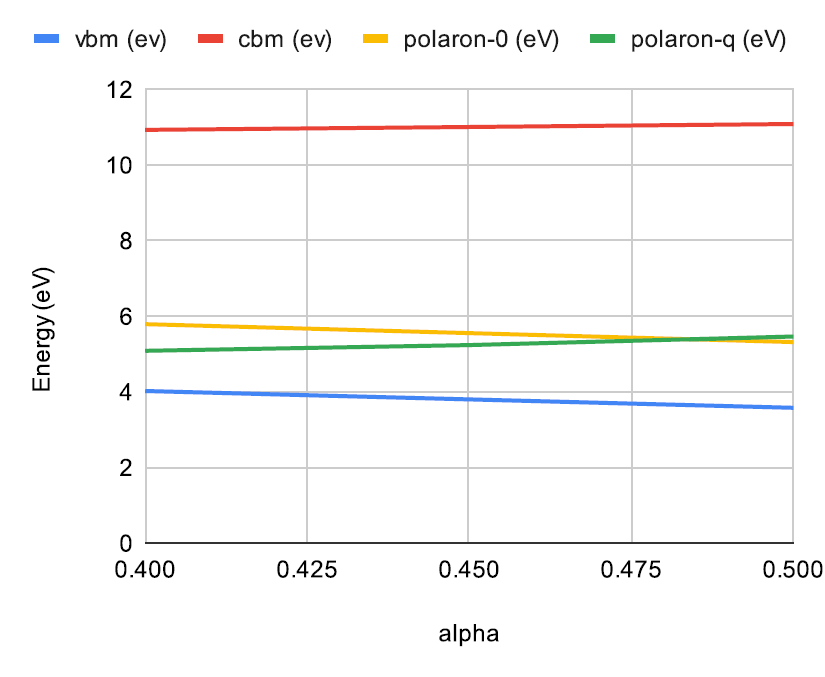
Figure S1: Energy levels of the valence band maximum (VBM), conduction band minimum (CBM), polaron level of the uncharged distorted system (polaron-0), and the polaron level of the charged distorted system (polaron-q) for MgO.

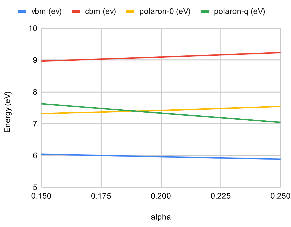
Figure S2: Energy levels of the valence band maximum (VBM), conduction band minimum (CBM), polaron level of the uncharged distorted system (polaron-0), and the polaron level of the charged distorted system (polaron-q) for BiVO4.

References

Sun et al. [2018]Q. Sun, T. C. Berkelbach, N. S. Blunt, G. H. Booth, S. Guo, Z. Li, J. Liu, J. D. McClain, E. R. Sayfutyarova, S. Sharma, S. Wouters, and G. K. L. Chan, PySCF: The Python-based simulations of chemistry framework, WIREs Comput. Mol. Sci. 8, 10.1002/wcms.1340 (2018).
Sun et al. [2020]Q. Sun, X. Zhang, S. Banerjee, P. Bao, M. Barbry, N. S. Blunt, N. A. Bogdanov, G. H. Booth, J. Chen, Z.-H. Cui, J. J. Eriksen, Y. Gao, S. Guo, J. Hermann, M. R. Hermes, K. Koh,
P. Koval, S. Lehtola, Z. Li, J. Liu, N. Mardirossian, J. D. McClain, M. Motta, B. Mussard, H. Q. Pham, A. Pulkin, W. Purwanto, P. J. Robinson, E. Ronca, E. R. Sayfutyarova, M. Scheurer, H. F. Schurkus,
J. E. T. Smith, C. Sun, S.-N. Sun, S. Upadhyay, L. K. Wagner, X. Wang, A. White, J. D. Whitfield, M. J. Williamson, S. Wouters, J. Yang, J. M. Yu, T. Zhu, T. C. Berkelbach, S. Sharma, A. Y. Sokolov, and G. K.-L. Chan, Recent developments in the PySCF program package, J. Chem. Phys. 153, 024109 (2020).
Falletta and Pasquarello [2022a]S. Falletta and A. Pasquarello, Polarons free from many-body self-interaction in density functional theory, Phys. Rev. B 106, 125119 (2022a).
Falletta and Pasquarello [2022b]S. Falletta and A. Pasquarello, Hubbard U through polaronic defect states, Npj Comput. Mater. 8, 10.1038/s41524-022-00958-6 (2022b).
Falletta and Pasquarello [2024]S. Falletta and A. Pasquarello, Nonempirical semilocal density functionals for correcting the self-interaction of polaronic states, J. Appl. Phys 135, 10.1063/5.0197658 (2024).