Robust Filter Design for Graph Signals

Abstract

Our goal in this paper is the robust design of filters acting on signals observed over graphs subject to small perturbations of their edges. The focus is on developing a method to identify spectral and polynomial graph filters that can adapt to the perturbations in the underlying graph structure while ensuring the filters adhere to the desired spectral mask. To address this, we propose a novel approach that leverages approximate closed-form expressions for the perturbed eigendecomposition of the Laplacian matrix associated with the nominal topology. Furthermore, when dealing with noisy input signals for graph filters, we propose a strategy for designing FIR filters that jointly minimize the approximation error with respect to the ideal filter and the estimation error of the output, ensuring robustness against both graph perturbations and noise. Numerical results validate the effectiveness of our proposed strategies, highlighting their capability to efficiently manage perturbations and noise.

I Introduction

Graph Signal Processing (GSP) [1], [2] has recently emerged as a powerful framework providing tools for the analysis and processing of data defined over graphs. Graph-based representations are pivotal tools for extracting information from data across various fields, ranging from finance, communication and social networks to biological sciences. While in certain contexts, such as physical networks, the graph topology might be perfectly known, in many others, the topology is completely unknown and has to be inferred from the observed data. Furthermore, there are situations where our knowledge of the graph topology is not perfect but affected by random uncertainties. For instance, in wireless communication networks, the topology is known, but some links may inadvertently drop due to random blocking or fading[3]. In such cases, we may only assume to know a nominal graph, whose topology may be perturbed by some random edge dropping. Similarly, in brain networks, the interaction among different regions of the brain changes over time [4],[5], and in biological networks, temporal variations of the network topology describing protein–protein and protein–DNA interactions are observed [6]. In data-driven networks, the topology is inferred from the data, and the learning accuracy depends on the inference algorithm as well as on the observed data that may be corrupted by noise or outliers. Therefore, it becomes interesting to analyze uncertain graphs, i.e., graphs wherein some edges may be altered with a certain probability.

Assuming that only a small percentage of edges remains uncertain, this paper aims to study the impact of small perturbations on the design of robust spectral and finite impulse response (FIR) filters acting on signals defined over graphs. Graph Filters (GFs) have been extensively studied in the literature [7], [8],[9]. Similarly, the stability of graph filters to perturbations has been thoroughly investigated in previous works [7], [10],[9] ,[11], [12]. A preliminary study on the impact of perturbations of graphs and simplicial complexes on the robustness of filters acting on signals observed over such domains is discussed in [13].
Recently, in [12] the authors introduced a novel approach that jointly addresses robust graph filter identification and graph denoising. In [14] the authors studied the stability of spectral GFs when a small number of edge were rewired. In [15] structural equation models are combined with total least squares to jointly infer signals and perturbations. Recently, the stability of Graph Convolutional Neural Networks (GCNs) has attracted increasing interest and has been the subject of extensive investigation in various works, e.g. [16],[17],[18], [19].
Our focus in this work is to design robust graph filters acting on signals defined over graphs that closely approximate the desired filter on the nominal graph, despite minor edge alterations. The proposed approach leverages the small perturbation analysis of the graph Laplacian eigenpairs developed in [20]. We use first-order closed form expressions for the perturbed Laplacian matrix eigenvalues/eigenvectors pairs to design graph filters that are robust against topology uncertainties. Then, we express robust filters in closed form, which depends only on the known probabilities of edge perturbations. Finally, in case where the filer input signals are affected by random noise, we introduce an optimization strategy aimed at finding a FIR filter that exhibits robustness both to graph perturbations and to noise interference. Specifically, the optimal FIR filter is designed to minimize, jointly, the approximation error respect to the desired (unperturbed) filter and the estimation error in the filter output. The effectiveness of the proposed strategies is substantiated through numerical results, demonstrating their good performance in handling both perturbations and noise.

II Small Perturbation Analysis of Graph Laplacian

In this section, first we quickly review some of the key tools for processing signals defined over graphs. Thereafter, we briefly recall the theory of small perturbation analysis of the graph Laplacian eigendecomposition developed in [20]. Let us consider an undirected graph $\mathcal{G}=\{\mathcal{V},\mathcal{E}\}$ composed of a set $\mathcal{V}=\{1,\ldots,N\}$ of $N$ nodes and a set $\mathcal{E}$ of edges, with cardinality $|\mathcal{E}|=E$. The connectivity of the graph can be described through the incidence matrix $\mbox{$\mathbf{B}$}_{1}\in\mathbb{N\times E}$, whose columns $\{\mathbf{b}_{m}\}_{m=1}^{E}$ establish which nodes are incident to each edge $m$. Specifically, given an arbitrary orientation of the edges, the entries of the column vector $\mathbf{b}_{m}$ are all zero except the entries $\mathbf{b}_{m}(i_{s})=1$ and $\mathbf{b}_{m}(i_{t})=-1$ corresponding to the indices $i_{s}$ and $i_{t}$ of the endpoints of edge $m$. The graph Laplacian $\mathbf{L}\in\mathbb{R}^{N\times N}$, is a symmetric, semidefinite positive matrix that captures the connectivity property of the graph and is defined as $\mbox{$\mathbf{L}$}=\mbox{$\mathbf{B}$}_{1}\mbox{$\mathbf{B}$}_{1}^{T}=\sum_{i\in\mathcal{E}}\mathbf{b}_{i}\mathbf{b}_{i}^{T}$. We assume, w.l.o.g., that the graph is connected and we denote with $\mbox{$\mathbf{L}$}=\mbox{$\mathbf{U}$}\boldsymbol{\Lambda}\mbox{$\mathbf{U}$}^{T}$ the Laplacian eigendecomposition, where $\mathbf{U}$ is the matrix whose columns are the eigenvectors $\mathbf{u}_{i}$, $i=1,\ldots,N$ and $\boldsymbol{\Lambda}$ is the diagonal matrix with entries the associated eiegenvalues $\lambda_{i}$, $i=1,\ldots,N$. We assume that the eigenvalues are listed in increasing order.
A signal $\mathbf{s}$ on a graph $\mathcal{G}$ is defined as a mapping from the vertex set to the set of real numbers, i.e. $\mathbf{s}:\mathcal{V}\rightarrow\mathbb{R}$. For undirected graphs, the GFT $\hat{\mathbf{s}}$ of a graph signal $\mathbf{s}$ is defined as the projection of $\mathbf{s}$ onto the subspace spanned by the eigenvectors $\mbox{$\mathbf{U}$}=\{\mathbf{u}_{i}\}_{i=1}^{N}$ of the Laplacian matrix, see e.g. [2], [21], i.e. $\hat{\mathbf{s}}=\mbox{$\mathbf{U}$}^{T}\mathbf{s}$.
Graph Small Perturbation Analysis. A small perturbation of the graph $\mathcal{G}$ corresponds to add or remove a few edges, thus resulting in the perturbed graph $\tilde{\mathcal{G}}$. Let us denote with $\mathcal{E}_{p}\subset\mathcal{E}$ the set of edges of the nominal graph that are altered. The perturbed graph is described by the perturbed Laplacian matrix $\widetilde{\mathbf{L}}=\mathbf{L}+\Delta\mathbf{L}$, where $\Delta\mathbf{L}\in\mathbb{R}^{N\times N}$ is a perturbation matrix that can be expressed as

$$\Delta\mathbf{L}=\sum_{m\in\mathcal{E}_{p}}\sigma_{m}\mathbf{b}_{m}\mathbf{b}_{m}^{T},$$ (1)

where $\sigma_{m}=1$ if edge $m$ is added and $\sigma_{m}=-1$, if edge $m$ is removed. Clearly, the perturbation of the nominal Laplacian $\mathbf{L}$ induces a perturbation of its eigenvalues decomposition denoted by

$$\widetilde{\mathbf{L}}=\mathbf{L}+\Delta\mathbf{L}=\widetilde{\mbox{$\mathbf{U}$}}\widetilde{\boldsymbol{\Lambda}}\widetilde{\mbox{$\mathbf{U}$}}^{T}$$ (2)

where $\widetilde{\mbox{$\mathbf{U}$}}:=\mbox{$\mathbf{U}$}+\Delta\mathbf{U}$ and $\widetilde{\boldsymbol{\Lambda}}:=\boldsymbol{\Lambda}+\Delta\boldsymbol{\Lambda}$ denote the eigenvector and the eigenvalues matrices of $\widetilde{\mathbf{L}}$. In the case where all eigenvalues are distinct and the perturbation affects a few percentage of edges, the perturbed eigenvectors $\{\widetilde{\mathbf{u}}_{i}\}_{i=1}^{N}$ and eigenvalues $\{\widetilde{\lambda}_{i}\}_{i=1}^{N}$ of $\widetilde{\mathbf{L}}$ are related to the unperturbed eigenvectors $\{\mathbf{u}_{i}\}_{i=1}^{N}$ and eigenvalues $\{\lambda_{i}\}_{i=1}^{N}$ of $\mathbf{L}$, by the following approximations [20]:

$$\widetilde{\lambda}_{i}\approx\lambda_{i}+\delta\lambda_{i}=\lambda_{i}+\mathbf{u}_{i}^{T}\Delta\mathbf{L}\mathbf{u}_{i}$$ (3)

$$\widetilde{\mathbf{u}}_{i}\approx\mathbf{u}_{i}+\delta\mathbf{u}_{i}=\mathbf{u}_{i}+\sum_{j\neq i}\frac{\mathbf{u}_{j}^{T}\Delta\mathbf{L}\mathbf{u}_{i}}{\lambda_{i}-\lambda_{j}}\mathbf{u}_{j}.$$ (4)

Therefore, from (II) and (4), the perturbations $\delta\lambda_{i}$ and $\delta\mathbf{u}_{i}$ of the $i$-th eigenvalue and eigenvector, respectively, can be written as [20]:

$$\begin{split}&\delta\lambda_{i}=\sum_{m\in\mathcal{E}_{p}}\sigma_{m}\mathbf{u}_{i}^{T}\mathbf{b}_{m}\mathbf{b}_{m}^{T}\mathbf{u}_{i}\end{split}$$ (5)

$$\begin{split}&\delta\mathbf{u}_{i}=\sum_{m\in\mathcal{E}_{p}}\sigma_{m}\delta\mathbf{u}_{im}\end{split}$$ (6)

with $\delta\mathbf{u}_{im}=\sum_{j\neq i}\frac{\mathbf{u}_{j}^{T}\mathbf{b}_{m}\mathbf{b}_{m}^{T}\mathbf{u}_{i}}{\lambda_{i}-\lambda_{j}}\mathbf{u}_{j}$. The above formulas come from a first-order perturbation analysis [20] which effectively captures the impact of the perturbation on the graph topology. In particular, the term $\mathbf{u}_{i}^{T}\mathbf{b}_{m}\mathbf{b}_{m}^{T}\mathbf{u}_{i}=(u_{i}(v_{s,m})-u_{i}(v_{t,m}))^{2}$ in (6) is a measure of the variation of the eigenvector $\mathbf{u}_{i}$ at the vertices $v_{s,m}$ and $v_{t,m}$ of edge $m$. Then, the largest perturbations occur over the edges that exhibit the highest eigenvectors variation. For example, in graphs characterized by dense clusters, the edges with most significant perturbations are the inter-cluster edges. Additionally, we can observe that the eigenvector corresponding to the null eigenvalue does not affect any other eigenvalue/eigenvector, and eigenvectors associated with eigenvalues very close to each other typically experience large perturbations.

III Robust Spectral Filtering over Perturbed Graphs

Our goal in this section is to design robust spectral filters for graphs that undergo small perturbation of their edges. In general, a spectral filter operating over a graph signal $\mathbf{s}_{0}$ can be modelled as

$$\mathbf{y}_{0}=\mbox{$\mathbf{H}$}\mbox{$\mathbf{s}$}_{0}$$ (7)

where $\mbox{$\mathbf{H}$}=\mbox{$\mathbf{U}$}\mbox{$\mathbf{D}$}\mbox{$\mathbf{U}$}^{T}$ and $\mathbf{D}$ is a diagonal matrix with entries the spectral mask coefficients $\{h(\lambda_{i})\}_{i=1}^{N}$ that we wish to implement over the eigenvalues of $\mathbf{L}$. Let us now assume that the graph topology is altered by either the addition or removal of a few edges. Then, using the closed-form expression in (4), we introduce the matrix $\tilde{\mbox{$\mathbf{U}$}}$ whose columns are the eigenvectors $\tilde{\mathbf{u}}_{i}$ of the perturbed Laplacian $\tilde{\mbox{$\mathbf{L}$}}$.
Our objective is to design a filter, denoted as $\tilde{\mbox{$\mathbf{H}$}}_{\mathbf{\tilde{D}}}=\tilde{\mbox{$\mathbf{U}$}}\tilde{\mbox{$\mathbf{D}$}}\tilde{\mbox{$\mathbf{U}$}}^{T}$, approximating with minimum averaged error the desired spectral mask $\mathbf{D}$, while being robust against small perturbation in the graph topology, such as the addition or removal of edges. Assuming that the perturbation of an edge $m$, is a random event characterized by a certain probability $p_{m}$, we describe this perturbation as a binary r.v. $Z_{m}$ equal to $1$, with probability $p_{m}$, if edge $m$ is perturbed, and $0$ otherwise. Then, let us consider the filter estimation error averaged with respect to random edge perturbations, i.e.

$$\mathbb{E}\left[\left\|\mathbf{U}\mathbf{D}\mathbf{U}^{T}-\tilde{\mathbf{U}}\tilde{\mathbf{D}}\tilde{\mathbf{U}}^{T}\right\|^{2}_{F}\right]=\mathbb{E}\left[\left\|\tilde{\mathbf{R}}-\tilde{\mathbf{D}}\right\|^{2}_{F}\right]$$ (8)

where $\tilde{\mathbf{R}}=\tilde{\mathbf{U}}^{T}\mathbf{U}\mathbf{D}\mathbf{U}^{T}\tilde{\mathbf{U}}$ and the last equality follows from the unitary property of $\tilde{\mathbf{U}}^{T}$.

Our goal is to derive the optimal spectral coefficients as solution of the following optimization problem

$$\begin{split}\min_{\tilde{\mathbf{D}}\in\mathbb{R}^{N\times N}}&\;f(\mathbf{\tilde{D}}):=\mathbb{E}\left[\left\|\tilde{\mathbf{R}}-\tilde{\mathbf{D}}\right\|^{2}_{F}\right]\\ \text{s.t.}&\quad\tilde{d}_{ij}=0,\quad\forall i\neq j\end{split}$$ (9)

where the constraints force the matrix $\tilde{\mbox{$\mathbf{D}$}}$ to be diagonal. Problem in (9) is convex and its optimal solution $\tilde{\mathbf{D}}^{\star}$ can be easily derived in closed-form by averaging with respect to the random edge perturbations. Specifically, the optimal $\tilde{\mathbf{D}}^{\star}$ is derived by taking the expectation of the diagonal elements of $\tilde{\mathbf{R}}$, i.e.

$$\mathbf{\tilde{D}}_{ii}^{\star}=\mathbb{E}[\tilde{\mathbf{R}}_{ii}],\quad i=1,\ldots,N.$$ (10)

To derive closed-form expressions for these optimal diagonal entries, let us recall that $\tilde{\mathbf{R}}=\tilde{\mathbf{U}}^{T}\mathbf{U}\mathbf{D}\mathbf{U}^{T}\tilde{\mathbf{U}}$. Then, using the equality $\mbox{$\mathbf{H}$}=\mbox{$\mathbf{U}$}\mbox{$\mathbf{D}$}\mbox{$\mathbf{U}$}^{T}$, we get $\tilde{\mathbf{R}}=\mathbf{\tilde{U}}\mathbf{H}\mathbf{\tilde{U}^{T}}$ and it holds

$$\tilde{\mathbf{D}}_{ii}^{\star}=\mathbb{E}[\tilde{\mathbf{u}}^{T}_{i}\mathbf{H}\tilde{\mathbf{u}}_{i}].$$ (11)

Assuming the random variables $Z_{m}$ and $Z_{n}$, i.i.d. for $m\neq n$, we get $\mathbb{E}[Z_{m}Z_{n}]=E[Z_{m}^{2}]=p_{m}$, if $m=n$ and $\mathbb{E}[Z_{m}Z_{n}]=p_{m}p_{n}$ if $m\neq n$. Then, using (4) and taking in (11) the expectation values with respect to the random variables $Z_{m}$, we easily derive the optimal solution

$$\tilde{\mathbf{D}}_{ii}^{\star}=\mathbf{u}_{i}^{T}\mathbf{H}\mathbf{u}_{i}+\!\sum_{k,l=1}^{N}\mathbf{H}_{k,l}\left(\sum_{m\in\mathcal{E}_{p}}p_{m}\delta\mathbf{u}_{i,m}(k)\delta\mathbf{u}_{i,m}(l)\right.$$ (12)

$$\left.+\sum_{m\in\mathcal{E}_{p}}\sum_{n\in\mathcal{E}_{p}}p_{m}p_{n}\sigma_{m}\sigma_{n}\delta\mathbf{u}_{i,m}(k)\delta\mathbf{u}_{i,n}(l)\right)$$

$$+2\mathbf{u}_{i}^{T}\mathbf{H}\left(\sum_{m\in\mathcal{E}_{p}}p_{m}\sigma_{m}\delta\mathbf{u}_{i,m}\right).$$

Note that the optimal spectral mask consists of a first term that represents the optimal solution for an unperturbed graph while the other terms take into account the perturbation statistics, enabling the mask to be adapted to random changes in the graph’s topology.

IV Robust Localized Filters

A desired graph filter $\mathbf{H}$ may be efficiently parameterized using a polynomial FIR filter of order $L$ based on the graph Laplacian as [7], [8]

$$\mbox{$\mathbf{H}$}=\sum_{k=0}^{L}h_{k}\mbox{$\mathbf{L}$}^{k}.$$ (13)

This is a local operator that combines graph signals from neighbors of each node, at a $k$-hop distance, through the coefficients $\{h_{k}\}_{k=0}^{L}$. Assuming that the graph undergoes random edge perturbations, our goal in this section is to design a robust FIR filter approximating with minimum averaged error the desired FIR filter $\mathbf{H}$ while being robust to small perturbations of the graph topology. Then, our aim is to derive the optimal filter $\tilde{\mbox{$\mathbf{H}$}}=\sum_{k=0}^{L}\tilde{h}_{k}\tilde{\mbox{$\mathbf{L}$}}^{k}$ with minimum average distance from the nominal filter $\mathbf{H}$ in (13). Hence, we may formulate the following optimization problem

$$\min_{\tilde{\mathbf{h}}\in\mathbb{R}^{L+1}}\;g(\tilde{\mathbf{h}}):=\mathbb{E}\left[\left\|\sum_{k=0}^{L}\tilde{h}_{k}\tilde{\mathbf{L}}^{k}-\sum_{n=0}^{L}h_{n}\mathbf{L}^{n}\right\|^{2}_{F}\right]$$ (14)

where the expectation is taken with respect to the random edge perturbations. Note that the objective function can be easily written as

$$\begin{split}g(\tilde{\mathbf{h}})=&\mathbb{E}\left[\left\|\sum_{k=0}^{L}\tilde{h}_{k}\tilde{\mathbf{U}}\tilde{\mathbf{\Lambda}}^{k}\tilde{\mathbf{U}}^{T}-\sum_{n=0}^{L}h_{n}\mathbf{U}\mathbf{\Lambda}^{n}\mathbf{U}^{T}\right\|^{2}_{F}\right]\\ =&\mathbb{E}\left[\left\|\sum_{k=0}^{L}\tilde{h}_{k}\tilde{\mathbf{\Lambda}}^{k}-\mathbf{M}\right\|^{2}_{F}\right],\\ \end{split}$$ (15)

where $\mathbf{M}=\tilde{\mathbf{U}}^{T}\mathbf{U}\left(\sum_{n=0}^{L}h_{n}\mathbf{\Lambda}^{n}\right)\mathbf{U}^{T}\tilde{\mathbf{U}}$. Then, defining the vector $\mathbf{m}=\text{diag}(\mathbf{M})$, whose entries are the diagonal elements of $\mathbf{M}$, the problem in (14) is equivalent to the following one

$$\min_{\tilde{\mathbf{h}}\in\mathbb{R}^{L+1}}\;\mathbb{E}[\|\mathbf{m}-\mathbf{\tilde{\Phi}}\tilde{\mathbf{h}}\|^{2}_{F}]$$ (16)

with $\mathbf{\tilde{\Phi}}=[\mathbf{1},\tilde{\boldsymbol{\lambda}},\ldots,\tilde{\boldsymbol{\lambda}}^{L}]$, $\tilde{\boldsymbol{\lambda}}^{k}=\{\tilde{\lambda}_{i}^{k}\}_{i=1}^{N}$, $k=1,\ldots,L$.

It can be easily shown that the optimal solution $\tilde{\mathbf{h}}^{\star}$ of the problem in (16) is given by

$$\tilde{\mathbf{h}}^{\star}=\mathbb{E}[\mathbf{\tilde{\Phi}}^{T}\mathbf{\tilde{\Phi}}]^{-1}\mathbb{E}[\mathbf{\tilde{\Phi}}^{T}\mathbf{m}].$$ (17)

Let us now derive a closed form expression for $\tilde{\mathbf{h}}^{\star}$ by taking the expectation with respect to the random edge perturbations. Note that it holds:

$$\mathbf{\tilde{\Phi}}^{T}\mathbf{\tilde{\Phi}}=\begin{bmatrix}N&\sum_{i=1}^{N}\tilde{\lambda}_{i}&\cdots&\sum_{i=1}^{N}\tilde{\lambda}_{i}^{L}\\ \vdots&\ddots&\vdots\\ \sum_{i=1}^{N}\tilde{\lambda_{i}}^{L}&\sum_{i=1}^{N}\tilde{\lambda_{i}}^{L+1}&\cdots&\sum_{i=1}^{N}\tilde{\lambda}_{i}^{2L}\end{bmatrix}.$$ (18)

From (5) we have $\delta\lambda_{i}=\sum_{m\in\mathcal{E}_{p}}Z_{m}q_{i,m}$ with $q_{i,m}=\mathbf{u}_{i}^{T}\mathbf{b}_{m}\mathbf{b}_{m}^{T}\mathbf{u}_{i}$. Then, we get the following expectation values

$$\mathbb{E}\left[\sum_{i=1}^{N}\tilde{\lambda}_{i}\right]=\sum_{i=1}^{N}(\lambda_{i}+\sum_{m\in\mathcal{E}_{p}}p_{m}\delta\lambda_{i,m})\vskip 6.0pt plus 2.0pt minus 2.0pt$$ (19)

$$\mathbb{E}\left[\sum_{i=1}^{N}\tilde{\lambda}_{i}^{k}\right]=\sum_{i=1}^{N}\sum_{j=0}^{k}\binom{k}{j}\lambda_{i}^{k-j}\mathbb{E}\left[(\delta\lambda_{i})^{j}\right]$$

where the term $\mathbb{E}\left[(\delta\lambda_{i})^{j}\right]=\mathbb{E}\left[(\sum_{m\in\mathcal{E}_{p}}Z_{m}q_{i,m})^{j}\right]$ can be easily calculated under the assumption of i.i.d. variables by using the equalities $\mathbb{E}[Z_{m}^{j}]=p_{m}^{j}$, $\forall m\in\mathcal{E}_{p}$ and $\mathbb{E}[Z_{r}Z_{s}\ldots Z_{j}]=p_{r}p_{s}\ldots p_{j}$ for any set of distinct indexes $r,s,\ldots,j$ within $\mathcal{E}_{p}$. Finally, let us consider the vector $\mathbb{E}[\mathbf{\tilde{\Phi}}^{T}\mathbf{m}]$ whose entries can be expressed as:

$$\mathbb{E}[(\mathbf{\tilde{\Phi}}^{T}\mathbf{m})_{i}] =\left(\sum_{n=0}^{L}h_{n}\lambda_{i}^{n}\right)\left(\sum_{p=1}^{N}\mathbf{u}_{i}(p)^{4}\mathbb{E}[(\lambda_{i}+\delta\lambda_{i})^{L}]\right.$$ (20)

$$+\mathbf{u}_{i}(p)^{2}\mathbb{E}[\delta\mathbf{u}_{i}(p)^{2}(\lambda_{i}+\delta\lambda_{i})^{L}]$$

$$+\left.2\mathbf{u}_{i}(p)^{3}\mathbb{E}[\delta\mathbf{u}_{i}(p)(\lambda_{i}+\delta\lambda_{i})^{L}]\right).$$

The first term of this sum can be simplified as in (19), the second term can be written as $\mathbb{E}[\delta\mathbf{u}_{i}(p)^{2}]\mathbb{E}[(\lambda_{i}+\delta\lambda_{i})^{L}]$, where $\mathbb{E}[\delta\mathbf{u}_{i}^{2}(p)]=\sum_{m\in\mathcal{E}_{p}}\sum_{n\in\mathcal{E}_{p}}\sigma_{m}\sigma_{n}\delta\mathbf{u}_{i,m}(k)\delta\mathbf{u}_{i,n}(l)p_{m}p_{n}$. Finally, we can write the third term as $2\mathbf{u}_{i}(p)^{3}\mathbb{E}[\delta\mathbf{u}_{i}(p)]\mathbb{E}[(\lambda_{i}+\delta\lambda_{i})^{L}]$, with $\mathbb{E}[\delta\mathbf{u}_{i}(p)]=\sum_{m\in\mathcal{E}_{p}}p_{m}\sigma_{m}\delta\mathbf{u}_{i,m}(p)$.

V Robust filtering for noisy signals and graph perturbations

In this section we focus on the robust filtering of noisy graph signals. Our goal is to find the optimal FIR filter which is robust against both graph perturbations and signal noise. Let us assume that the filter’s input graph signal $\mathbf{x}$ is affected by random noise $\mathbf{n}$ and define $\mbox{$\mathbf{y}$}=\mbox{$\mathbf{x}$}+\mathbf{n}$ as the noisy signal we aim to filter. Then, in the case where the graph is perturbed and the signal is affected by noise, the filtered signal is given by $\tilde{\mbox{$\mathbf{z}$}}=\tilde{\mbox{$\mathbf{H}$}}\mbox{$\mathbf{y}$}$. Then, we are interested in finding optimal coefficients that minimize jointly the approximation error respect to the desired (unperturbed) filter $\mathbf{H}$, i.e. $g(\tilde{\mathbf{h}})$ in (14), and the estimation error in the perturbed filter output with respect to the ideal output $\mathbf{H}$$\mathbf{x}$. Hence, we may formulated the following optimization problem:

$$\begin{split}\min_{\tilde{\mathbf{h}}\in\mathbb{R}^{L+1}}\;&\mathbb{E}\left[\left\|\sum_{k=0}^{L}\tilde{h}_{k}\tilde{\mathbf{L}}^{k}-\sum_{n=0}^{L}h_{n}\mathbf{L}^{n}\right\|^{2}_{F}\right]\\ &+\gamma\,\mathbb{E}\left[\left\|\sum_{k=0}^{L}\tilde{h}_{k}\tilde{\mathbf{L}}^{k}\mbox{$\mathbf{y}$}-\sum_{n=0}^{L}h_{n}\mathbf{L}^{n}\mbox{$\mathbf{x}$}\right\|^{2}_{F}\right]\end{split}$$ (21)

where $\gamma$ is a non-negative coefficient to control the trade-off between the two estimation errors. Note that the optimization problem in (21) can be written in the following equivalent form

$$\min_{\tilde{\mathbf{h}}\in\mathbb{R}^{L+1}}\;\mathcal{L}(\tilde{\mathbf{h}}):=\mathbb{E}[\|\mathbf{m}-\mathbf{\tilde{\Phi}}\tilde{\mathbf{h}}\|^{2}_{F}]+\gamma\,\mathbb{E}[\|{\mathbf{w}}-\mbox{$\mathbf{D}$}_{y}\mathbf{\tilde{\Phi}}\tilde{\mathbf{h}}\|^{2}_{F}]$$ (22)

where $\mathbf{w}=\tilde{\mbox{$\mathbf{U}$}}^{T}\mbox{$\mathbf{U}$}(\sum_{n=0}^{L}h_{n}\boldsymbol{\Lambda}^{n})\mbox{$\mathbf{U}$}^{T}\mathbf{x}$ and $\mbox{$\mathbf{D}$}_{y}=\text{diag}(\hat{\mathbf{y}})$ with $\mathbf{\hat{y}}=\mathbf{\tilde{U}}^{T}\mathbf{y}$. The objective function $\mathcal{L}(\tilde{\mathbf{h}})$ of the problem in (22) can be expressed as

$$\mathcal{L}(\tilde{\mathbf{h}}) =\mathbb{E}\Bigl{[}\text{tr}\Bigl{\{}\mathbf{m}^{T}\mathbf{m}+\mathbf{\tilde{h}}^{T}\mathbf{\tilde{\Phi}}^{T}\mathbf{\tilde{\Phi}}\mathbf{\tilde{h}}-2\mathbf{\tilde{h}}^{T}\mathbf{\tilde{\Phi}}^{T}\mathbf{m}\Bigr{\}}\Bigr{]}+$$ (23)

$$\gamma\mathbb{E}\Bigl{[}\text{tr}\Bigl{\{}\mathbf{w}^{T}\mathbf{w}+\mathbf{\tilde{h}}^{T}\mathbf{\tilde{\Phi}}^{T}\mathbf{D}_{y}^{2}\mathbf{\tilde{\Phi}}\mathbf{\tilde{h}}-2\mathbf{{\tilde{h}}}^{T}\mathbf{\tilde{\Phi}}^{T}\mathbf{D}_{y}\mathbf{w}\Bigr{\}}\Bigr{]}$$

from which the optimal solution $\mathbf{\tilde{h}}$ can be derived in closed form as

$$\mathbf{\tilde{h}}=\mathbb{E}\Bigl{[}\mathbf{\tilde{\Phi}}^{T}\mathbf{\tilde{\Phi}}+\gamma\mathbf{\tilde{\Phi}}^{T}{\mathbf{D}}_{y}^{2}\mathbf{\tilde{\Phi}}\Bigr{]}^{-1}\mathbb{E}\Bigl{[}\mathbf{\tilde{\Phi}}^{T}(\mathbf{m}+\gamma\mathbf{D}_{y}\mathbf{w})\Bigr{]}.$$ (24)

Following similar derivations as in (19) and (20), closed form solutions can be obtained, which we omit here due to space constraints.

VI Numerical Results

In this section, we validate the effectiveness of the proposed filtering designs through comprehensive numerical experiments.
To evaluate the robustness of both spectral and FIR filters against perturbed graphs, we generated $100$ random realizations of graphs, each consisting of two clusters. These graphs have an intra-cluster and inter-cluster connection probability equal to $0.7$ and $0.08$, respectively. We randomly perturbed a varying percentage of the total edges, from $1\%$ to $20\%$, ensuring that after perturbations the graph remains connected. Using the closed-form formulas in (12), (19) and (20), we derived, respectively, the optimal mask $\tilde{\mathbf{D}}^{\star}$ and the optimal FIR coefficients $\tilde{\mathbf{h}}^{\star}$. Then, we calculated for both filters the associated average distances between the desired and estimated filters, i.e. $f(\tilde{\mbox{$\mathbf{D}$}}^{\star})$ and $g(\tilde{\mathbf{h}}^{\star})$, respectively. In Fig. 1, we report these average distances versus the percentage of perturbed edges. Furthermore, to assess the robustness of our proposed optimal filters, we also report in Fig. 1 the average distance between the ideal target filter and the non-optimized filters (NOF) where the filter coefficients are directly derived using the perturbed graph, for both the spectral and FIR filters. It is evident the robustness enhancement achieved using the proposed optimal filtering design. However, the spectral filtering approach exhibits more robustness, due to the fact that the FIR filter is a polynomial approximation of the intended one.

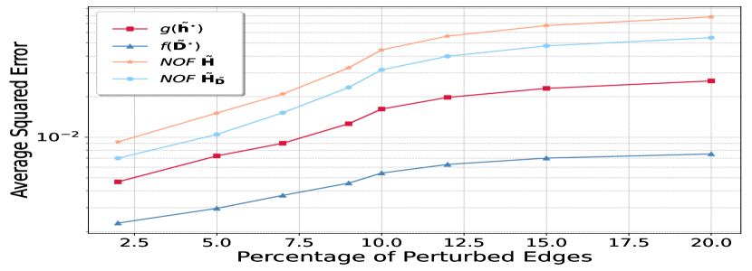
Figure 1: Average squared errors vs the percentage of perturbed edges.

Let us now consider the robust filtering of noisy signals. In order to generalize our findings, in this experiment we employed Erdős–Rényi graphs. We generated $100$ different graphs, each containing $100$ nodes, with a connection probability of $p=0.5$ for each edge, ensuring that the graphs remain connected after the perturbations. Then, by solving the problem in (21), let us denote with $\mathbf{D}(\mathbf{L},\mathbf{\tilde{L}}^{\star})$ and $\mathbf{D}_{xy}(\mathbf{L},\mathbf{\tilde{L}}^{\star})$ the optimal (normalized) values of the first and second term of the objective function. In Fig. 2 we report the optimal distance $\mathbf{D}_{xy}(\mathbf{L},\mathbf{\tilde{L}}^{\star})$, representing the estimation error in the perturbed filter output, versus the noise variance $\sigma_{n}^{2}$ and for various levels of perturbation. We can observe as increasing the variance of the noise, $\mathbf{D}_{xy}$ increases as well, albeit it maintains robustness for small perturbation levels.
Finally, in Fig. 3 we illustrate the trade-off between the two terms, $\mathbf{D}_{xy}(\mathbf{L},\mathbf{\tilde{L}}^{\star})$ and $\mathbf{D}(\mathbf{L},\mathbf{\tilde{L}}^{\star})$, by varying the penalty coefficient $\gamma$. It can be observed as the optimal filter approximation error (respect to the desired filter) and the optimal estimation error in the perturbed filter output exhibit robustness across various percentages of edges perturbations.

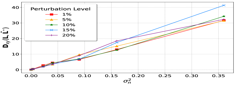
Figure 2: Average distance $\mathbf{D}_{xy}(\mathbf{L},\mathbf{\tilde{L}}^{\star})$ vs the noise variance $\sigma_{n}^{2}$.

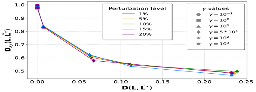
Figure 3: Trade-off between $\mathbf{D}(\mathbf{L},\mathbf{\tilde{L}}^{\star})$ and $\mathbf{D}_{xy}(\mathbf{L},\mathbf{\tilde{L}}^{\star})$ varying $\gamma$.

VII Conclusions

In this paper we consider the robust design of filters for signals observed over graphs that may undergo random small perturbations of their topology. Our objective is to devise a strategy for deriving spectral and polynomial filters that can adapt to small changes in the graph’s topology, while still closely approximating the desired spectral mask. To this end, we introduce an innovative approach that utilizes approximate closed-form solutions for the perturbed eigendecomposition of the graph Laplacian matrix. Additionally, we propose a strategy to find optimal filters that are jointly robust against the random graph perturbations and the signal noise.

References

- [1] A. Ortega, P. Frossard, J. Kovačević, J. M. F. Moura, and P. Vandergheynst, “Graph signal processing: Overview, challenges, and applications,” Proc. of the IEEE, vol. 106, no. 5, pp. 808–828, May 2018.
- [2] D. I. Shuman, S. K. Narang, P. Frossard, A. Ortega, and P. Vandergheynst, “The emerging field of signal processing on graphs: Extending high-dimensional data analysis to networks and other irregular domains,” IEEE Signal Process. Mag., vol. 30, no. 3, pp. 83–98, May 2013.
- [3] J. Ghosh, H. Q. Ngo, S. Yoon, and C. Qiao, “On a routing problem within probabilistic graphs and its application to intermittently connected networks,” in Proc. 26th IEEE Int. Conf. on Comp. Commun. (INFOCOM), 2007, pp. 1721–1729.
- [4] V. D. Calhoun, R. Miller, G. Pearlson, and T. Adalı, “The chronnectome: time-varying connectivity networks as the next frontier in fmri data discovery,” Neuron, vol. 84, no. 2, pp. 262–274, 2014.
- [5] M. G. Preti, T. A.W. Bolton, and D. Van De Ville, “The dynamic functional connectome: State-of-the-art and perspectives,” Neuroimage, vol. 160, pp. 41–54, 2017.
- [6] Y. Kim, S. Han, S. Choi, and D. Hwang, “Inference of dynamic networks using time-course data,” Brief. in Bioinform., vol. 15, no. 2, pp. 212–228, 2014.
- [7] A. Sandryhaila and J. M. F. Moura, “Discrete signal processing on graphs: Frequency analysis,” IEEE Trans. Signal Process., vol. 62, no. 12, pp. 3042–3054, June 2014.
- [8] S. Segarra, A. G. Marques, and A. Ribeiro, “Optimal graph-filter design and applications to distributed linear network operators,” IEEE Trans. Signal Process., vol. 65, no. 15, pp. 4117–4131, Aug. 2017.
- [9] J. Liu, E. Isufi, and G. Leus, “Filter design for autoregressive moving average graph filters,” IEEE Trans. Signal Inform. Process. over Netw., vol. 5, no. 1, pp. 47–60, 2018.
- [10] F. Gama, E. Isufi, G. Leus, and A. Ribeiro, “Graphs, convolutions, and neural networks: From graph filters to graph neural networks,” IEEE Signal Process. Mag., vol. 37, no. 6, pp. 128–138, 2020.
- [11] L. Ben Saad, B. Beferull-Lozano, and E. Isufi, “Quantization analysis and robust design for distributed graph filters,” IEEE Trans. Signal Process., vol. 70, pp. 643–658, 2022.
- [12] S. Rey, V. M. Tenorio, and A. G. Marqués, “Robust graph filter identification and graph denoising from signal observations,” IEEE Trans. on Signal Process., vol. 71, pp. 3651–3666, 2023.
- [13] S. Sardellitti and S. Barbarossa, “Robust signal processing over simplicial complexes,” in ICASSP 2022-2022 IEEE Inter. Conf. Acoust., Speech and Signal Process. (ICASSP). IEEE, 2022, pp. 8857–8861.
- [14] H. Kenlay, D. Thanou, and X. Dong, “Interpretable stability bounds for spectral graph filters,” in Inter. Conf. on Machine Learn. PMLR, 2021, pp. 5388–5397.
- [15] E. Ceci, Y. Shen, G. B. Giannakis, and S. Barbarossa, “Graph-based learning under perturbations via total least-squares,” IEEE Trans. on Signal Process., vol. 68, pp. 2870–2882, 2020.
- [16] F. Gama, J. Bruna, and A. Ribeiro, “Stability properties of graph neural networks,” IEEE Trans. Signal Process., vol. 68, pp. 5680–5695, 2020.
- [17] N. Keriven, A. Bietti, and S. Vaiter, “Convergence and stability of graph convolutional networks on large random graphs,” in Advan. in Neur. Inform. Process. Systems, H. Larochelle, M. Ranzato, R. Hadsell, M.F. Balcan, and H. Lin, Eds. 2020, vol. 33, pp. 21512–21523, Curran Associates, Inc.
- [18] R. Levie, W. Huang, L. Bucci, M. Bronstein, and G. Kutyniok, “Transferability of spectral graph convolutional neural networks,” Jour. of Mach. Learn. Resear., vol. 22, no. 272, pp. 1–59, 2021.
- [19] L. Testa, C. Battiloro, S. Sardellitti, and S. Barbarossa, “Stability of graph convolutional neural networks through the lens of small perturbation analysis,” 2023.
- [20] E. Ceci and S. Barbarossa, “Graph signal processing in the presence of topology uncertainties,” IEEE Trans. Signal Process., vol. 68, pp. 1558–1573, 2020.
- [21] I. Pesenson, “Sampling in Paley-Wiener spaces on combinatorial graphs,” Trans. Amer. Math. Soc., vol. 360, no. 10, pp. 5603–5627, Oct. 2008.