State-Augmented Linear Games with Antagonistic Error for High-Dimensional, Nonlinear Hamilton-Jacobi Reachability

Abstract

Hamilton-Jacobi Reachability (HJR) is a popular method for analyzing the liveness and safety of a dynamical system with bounded control and disturbance. The corresponding HJ value function offers a robust controller and characterizes the reachable sets, but is traditionally solved with Dynamic Programming (DP) and limited to systems of dimension less than six. Recently, the space-parallelizeable, generalized Hopf formula has been shown to also solve the HJ value with a nearly three-log increase in dimension limit, but is limited to linear systems. To extend this potential, we demonstrate how state-augmented (SA) spaces, which are well-known for their improved linearization accuracy, may be used to solve tighter, conservative approximations of the value function with any linear model in this SA space. Namely, we show that with a representation of the true dynamics in the SA space, a series of inequalities confirms that the value of a SA linear game with antagonistic error is a conservative envelope of the true value function. It follows that if the optimal controller for the HJ SA linear game with error may succeed, it will also succeed in the true system. Unlike previous methods, this result offers the ability to safely approximate reachable sets and their corresponding controllers with the Hopf formula in a non-convex manner. Finally, we demonstrate this in the slow manifold system for clarity, and in the controlled Van der Pol system with different lifting functions.

I Preamble

Verifying that a system satisfies safety or goal-satisfaction specifications for nonlinear systems with bounded control and disturbance inputs is a crucial yet computationally challenging task. Hamilton-Jacobi reachability (HJR) analysis is a formal verification tool for guaranteeing the performance and safety of such systems. HJR first defines a cost function encodes a target set of states to either reach or avoid, and then solves a differential game backward in time between the control and disturbance inputs, assuming the latter is adversarial. The result is a value function that encodes the backward reachable set (BRS): the set of states from which the controller may drive the system into the target despite any disturbance (for the Reach problem), or where the optimal control will fail to ultimately avoid the target for the worst-case disturbance (for the Avoid problem). Moreover, the corresponding optimal control policy in either case may be solved from the gradient of the value function.

HJR has been widely applied in numerous safety-critical applications [1, 2] due to its ability to produce strong guarantees. However, HJR relies on dynamic programming (DP), which suffers from exponential compute burden with respect to dimension (i.e., the curse of dimensionality). In practice, DP is unable to solve HJ problems with systems of greater than three dimensions online and six offline. Several works have sought to improve scalability via learning methods [2, 3], linearization [4, 5], and decomposition [6, 7], but scalability remains a challenge when deterministic guarantees are required.

Solving differential games with linear dynamics and bounded inputs is more tractable due to the recent application of the generalized Hopf formula [8, 9]. If the target is convex, by a change of coordinates with the fundamental matrix, the value function may be solved independently in space by optimization over the space of the costate. This allows the game value (and optimal control) to be rapidly solved for a single point in space and time without the exponential burden, and experimentally, has allowed computation of systems of up to dimension 4096 to be solved in milliseconds [10]. The major limitation is that the system must be linear for the validity of the generalized Hopf formula.

To apply the Hopf formula to nonlinear systems, standard linearizations have been used successfully in multi-agent pursuit-evasion games [4], in an LQR-like iterative fashion [5], and by approximating the Koopman operator [11]. Despite empirical success, none of these approaches provide conservative guarantees on the value. Recently, it was shown that a conservative solution may be derived by transforming the error between any linear model and the nonlinear system into an antagonistic player, providing a conservative envelope of the true HJR value function [12]. This approach provides the necessary guarantees for safety-critical systems, but tends to be overly conservative for long time horizons or highly nonlinear systems.

In this work, we generalize the results in [12] to state-augmented (SA) systems. SA systems are popular for their ability to significantly outperform standard linearizations [13], and appear in, e.g., extended dynamic mode decomposition (EDMD) [14], learning-based linearizations [15, 16] and in other approximations of the Koopman Operator [17, 18, 19]. It is well-known that in the (asymptotic) limit of increasing dimension, the map of certain “lifted” models approaches the action of the Koopman Operator [20, 21, 22] which exactly captures the nonlinear dynamics [23].

In this paper, we define a differential game with antagonistic error for any SA linear model whose value at true states mapped to the SA space is guaranteed to be conservative with respect to the true solution (Theorem  2). The proof follows from a series of value function comparisons and may be found in Sec. IV. An immediate corollary is that reachability in the SA linear game with error implies the optimal control policy derived from the corresponding SA HJ value function is guaranteed to succeed in the original nonlinear system despite any true disturbance or error of the SA model (23). We demonstrate the result in detail with the slow-manifold system in Sec.V-A, which famously has an exact SA linear representation in the autonomous case; in the case with inputs, the linear model is inexact, and we show the augmented value function offers conservative envelopes (Figure 1). Finally, we demonstrate in the controlled Van der Pol system in Sec.V-B how these results may be applied with various lifting functions to observe their corresponding conservative envelopes of the true solution where the controller is guaranteed to succeed (Figure 2).

The contributions of this work include:

1. a novel Hopf-amenable method for generating conservative envelopes of HJ value functions via a SA linear game with antagonistic error,

2. a formal proof that the resulting controller and reachable set are conservative for both the performance (Reach) and safety (Avoid) problem formulations, and

3. demonstrations with comparison to traditional DP-based HJR, and with various lifting functions.

II Preliminaries

This paper focuses on control-affine and disturbance-affine systems of the form

$$\dot{x}=f_{x}(x)+h_{1}(x)u+h_{2}(x)d\triangleq f(x,u,d)$$ (1)

with state $x\in\mathcal{X}\triangleq\mathbb{R}^{n_{x}}$, and control $u$ and disturbance $d$ drawn from compact & convex sets $\mathcal{U}\subseteq\mathbb{R}^{n_{u}}$, $\mathcal{D}\subseteq\mathbb{R}^{n_{d}}$. Let the input signals $u(\cdot)$ and $d(\cdot)$ be drawn from $\mathbb{U}(t)\triangleq\{\nu:[t,T]\mapsto\mathcal{U}\mid\nu\text{ measurable}\}$ and $\mathbb{D}(t)\triangleq\{\nu:[t,T]\to\mathcal{D}\mid\nu\text{ measurable}\}$. Let $f$ be Lipschitz continuous in $(x,u,d)$ s.t. there exists a unique trajectory $\xi_{f}:[t,T]\to\mathcal{X}$ of $f$ defined by $\xi_{f}(t)=x$ and $\dot{\xi_{f}}(\tau)=f(\xi_{f}(\tau),u(\tau),d(\tau))$ a.e. for $\tau\in[t,T]$. For clarity, we at times write $\xi_{f}(\tau;x,u(\cdot),d(\cdot),t)$.

II-A Hamilton-Jacobi Reachability Problem

To design a safe autonomous controller, HJR solves the optimal control that counters an adversarial disturbance in a differential game. The game is defined by the cost functional,

$$C(x,u(\cdot),d(\cdot),t)\triangleq J(\xi_{f}(T))+\int_{t}^{T}L(u(\tau),d(\tau))d\tau,$$ (2)

which scores a trajectory for given input signals. Let the Reach game be defined as the problem where the objective of Player I, the control, is to minimize (2) while the objective of Player II, the disturbance, seeks to maximize it. Let the Avoid game be defined s.t. the objectives of players are swapped.

The terminal cost $J:\mathcal{X}\to\mathbb{R}$ is a convex, proper, lower semicontinuous function chosen such that

$$\begin{cases}J(x)<0\>\>\text{ for }\>\>x\in\mathcal{T}\setminus\partial\mathcal{T}\\ J(x)=0\>\>\text{ for }\>\>x\in\partial\mathcal{T}\\ J(x)>0\>\>\text{ for }\>\>x\notin\mathcal{T}\\ \end{cases}$$ (3)

where $\mathcal{T}\in\mathcal{X}$ is a user-defined, closed set representing the target to reach or avoid and $\partial\mathcal{T}$ is its boundary. To allow any feasible inputs to guide or perturb the trajectory, we assume the running cost $L\equiv 0$ in this work, but the derived conservative guarantee of the value may apply for any convex $L$ [8, 9] but no longer characterizes reachability. In this context, we have defined the cost such that it has the property,

$$\begin{aligned} C(x,u(\cdot),d(\cdot),t)\leq 0&\iff J(\xi_{f}(T)\leq 0\\ &\iff\xi_{f}(T)\in\mathcal{T},\end{aligned}$$ (4)

where $\xi_{f}(T)=\xi_{f}(T;x,u(\cdot),d(\cdot),t)$.

Consider the game in which the disturbance has an instantaneous information advantage, but plays with respect to previous observations only. Formally, let a strategy $\mathfrak{d}:\mathbb{U}(t)\to\mathbb{D}(t)$ for Player II be drawn from the set of non-anticipative strategies [24, 25, 1],

$$\begin{aligned} \mathfrak{d}\in\mathfrak{D}(t)\triangleq\{\gamma\mid u(\tau)=\hat{u}(\tau),\text{ a.e. }\tau\in[t,T]\implies\\ \mathfrak{d}[u](\tau)=\mathfrak{d}[\hat{u}](\tau),\text{ a.e. }\tau\in[t,T]\}.\end{aligned}$$ (5)

Then the value functions $V,V^{-}:\mathcal{X}\times(-\infty,T]\to\mathbb{R}$ corresponding to the values of the Reach and Avoid games resp. are defined as

$$\begin{aligned} V(x,t)&\triangleq\sup_{\mathfrak{d}\in\mathfrak{D}(t)}\inf_{u(\cdot)\in\mathbb{U}(t)}J(\xi_{f}(T;x,u(\cdot),\mathfrak{d}[u](\cdot),t)),\\ V^{-}(x,t)&\triangleq\inf_{\mathfrak{d}\in\mathfrak{D}(t)}\sup_{u(\cdot)\in\mathbb{U}(t)}J(\xi_{f}(T;x,u(\cdot),\mathfrak{d}[u](\cdot),t)).\end{aligned}$$ (6)

At times, we write $V(x,t;f,\mathcal{T})$ to clarify this definition. Analogous to (4), these functions have the sublevel property,

$$\begin{aligned} V(x,t)&\leq 0\iff x\in\mathcal{R}(\mathcal{T},t),\\ V^{-}(x,t)&\leq 0\iff x\in\mathcal{R}^{-}(\mathcal{T},t)\end{aligned}$$ (7)

where $\mathcal{R}(\mathcal{T},t)$ & $\mathcal{R}^{-}(\mathcal{T},t)$ are the backward reachable sets (BRSs): the set of states which may be driven to the target at time $T$ (starting from time $t$) despite any disturbance (Reach set) or despite any control (Avoid set) respectively,

$$\begin{aligned} \mathcal{R}(\mathcal{T},t)\triangleq\{x\mid\forall\mathfrak{d}\in\mathfrak{D}(t),\exists u(\cdot)\in\mathbb{U}(t)\text{ s.t. }\\ \xi_{f}(T;x,u(\cdot),\mathfrak{d}[u](\cdot),t)\in\mathcal{T}\},\\ \mathcal{R}^{-}(\mathcal{T},t)\triangleq\{x\mid\exists\mathfrak{d}\in\mathfrak{D}(t),\forall u(\cdot)\in\mathbb{U}(t)\text{ s.t. }\\ \xi_{f}(T;x,u(\cdot),\mathfrak{d}[u](\cdot),t)\in\mathcal{T}\}.\end{aligned}$$ (8)

In contrast, consider the set of all backwards feasible states $\mathcal{S}\subseteq\mathcal{X}$ for which there exist bounded input signals that could drive the trajectory into the target at time $T$ starting from time $t$, given by

$$\begin{aligned} \mathcal{S}(\mathcal{T},t)\triangleq\{x\mid\exists u(\cdot)\in\mathbb{U}(t),\quad\exists d(\cdot)\in\mathbb{D}(t)\text{ s.t. }\\ \xi_{f}(T;x,u(\cdot),d(\cdot),t)\in\mathcal{T}\}.\end{aligned}$$ (9)

By Filippov and others, this set will be bounded for any compact sets $\mathcal{T}$, $\mathcal{U}$, $\mathcal{D}$ and Lipschitz dynamics [26, 27, 28]. Additionally, the backwards feasible tube $\bar{\mathcal{S}}$ will be a relevant object for bounding trajectories of the game and is given by

$$\begin{aligned} \bar{\mathcal{S}}(\mathcal{T},t)\triangleq\bigcup_{\tau\in[t,T]}\mathcal{S}(\mathcal{T},\tau),\end{aligned}$$ (10)

which we may also know is bounded given the above assumptions for the closed interval $[t,T]$. In antagonistic or worst-case scenarios, $\mathcal{S}$ & $\bar{\mathcal{S}}$ are insufficient for guaranteeing $\xi_{f}(T)\in\mathcal{T}$, however, they may be used for bounding trajectories in order to define an antagonistic error player [12], which offers a conservative guarantee for a linear game with respect to a nonlinear game.

Notably, applying Bellman’s principle of optimality to the value function $V$ leads to the following well-known theorem.

Theorem 1 (Evans 84).

[25]
Given the assumptions (2.1)-(2.5) in [Evan 84], the value function $V$ defined in (6) is the viscosity solution to the following Hamilton-Jacobi Partial Differential Equation,

$$\begin{aligned} \dot{V}+H(x,\nabla_{x}V,\tau)&=0&\text{ on }\mathcal{X}&\times[t,T],\\ V(x,T)&=J(\xi_{f}(T))&\text{ on }\mathcal{X}&\end{aligned}$$ (11)

where the Hamiltonian $H:\mathcal{X}\times\mathcal{X}\times[t,T]\to\mathbb{R}$ is

$$H(x,p,t)=\min_{u\in\mathcal{U}}\max_{d\in\mathcal{D}}p\cdot f(x,u,d).$$ (12)

This equivalently applies to $V^{-}$, but note that the Hamiltonian in the Avoid game takes the flipped form $H^{-}(x,p,t)=\max_{u}\min_{d}p\cdot f(x,u,d)$. In either game, solving this PDE yields the value function and corresponding BRS. Additionally, the value function can be used to derive the optimal control policy for $(x,t)$, e.g., for the Reach game:

$$\begin{aligned} u^{*}(\tau)=\arg\min_{u\in\mathcal{U}}\nabla_{x}V(\xi_{f}(\tau;x),\tau)\cdot h_{1}(\tau)u.\end{aligned}$$ (13)

The main challenge of HJR lies in solving the PDE in (11); DP methods propagate $V(x,t)$ by finite-differences over a grid of points that grows exponentially with respect to ${n_{x}}$ [2]. In practice, this is computationally intractable for systems with dimension ${n_{x}}\geq 6$ and is constrained to offline analysis.

Notably, it has been shown in [29, 8, 9] that if a system has linear dynamics and the target is convex, then the generalized Hopf formula [30] gives the viscosity solution of (11). Hence, instead of DP, the value may be feasibly solved by optimization of the Hopf formula independently over space, and this has been demonstrated for systems of up to dimension ${n_{x}}=4096$ [31]. However, this is limited to linear dynamics and motivates the current work.

II-B State Augmented Systems

Consider an augmentation of the space $\mathcal{X}$, say $\mathcal{G}\triangleq\mathbb{R}^{{n_{k}}}$. Namely, let the lifting function $\Psi:\mathcal{X}\to\mathcal{G}$ be a bounded map from the state space to the augmented space that takes the following form,

$$\Psi(x)\triangleq[x,\psi_{1}(x),\dots,\psi_{{n_{k}}-{n_{x}}}(x)]^{\top},\psi_{i}:\mathcal{X}\to\mathbb{R}$$ (14)

where $\psi_{i}\in C^{1}$ are smooth, user-defined functions that are chosen to improve the linearization accuracy, e.g. a truncated functional basis. The range ${\mathscr{R}}_{\Psi}\subseteq\mathcal{G}$ represents a manifold in the augmented space (see, for example, Figure 1). By definition, $\Psi$ is injective and therefore has an inverse in the range, say ${\Psi}^{-1}:{\mathscr{R}}_{\Psi}\to\mathcal{X}$ with ${\Psi}^{-1}(g)\triangleq x$ if $g=\Psi(x)$.

Let the map $P:\mathcal{G}\to\mathcal{X}$ be the projection of the augmented space onto the state space, which in this context takes the form of a matrix $P=[I_{n_{x}}\>0_{{n_{k}}-{n_{x}}}]$. By definition,

$$x=P\Psi(x),\text{ hence }{\Psi}^{-1}=P|_{{\mathscr{R}}_{\Psi}}$$ (15)

where $P|_{{\mathscr{R}}_{\Psi}}:{{\mathscr{R}}_{\Psi}}\to\mathcal{X}$ is the restriction of the map to the manifold.

Additionally, consider a linear model in $\mathcal{G}$,

$$\dot{g}\approx\kappa(g,u,d)\triangleq Kg+L_{1}u+L_{2}d.$$ (16)

where $K,L_{1},L_{2}\in\mathbb{R}^{{n_{k}}\times{n_{k}}},\mathbb{R}^{{n_{k}}\times n_{u}},\mathbb{R}^{{n_{k}}\times n_{d}}$ are real matrices. This system may be generated in a variety of ways, including, e.g., via the taylor series or least-squares fitting. The principal result will hold for any finite linear model, since a finite linear map is bounded, yielding a finite maximum error on the bounded set $\bar{\mathcal{S}}$ [12]. In the original space, this error may be large, giving overly conservative guarantees for long time-horizons or highly-nonlinear systems, but in SA systems, it is well-known that in the limit of increasing dimension, there are linear models whose output will approach the action of the Koopman operator asymptotically [20, 21, 22].

III RESULTS

In this section, we state the main theoretical result, namely that the true nonlinear game value may be conservatively approximated by a linear game value with antagonistic error in the state augmented system. Toward defining this latter game, let the augmented target $\mathcal{T}_{\mathcal{G}}$ be defined as,

$$\mathcal{T}_{\mathcal{G}}\triangleq\{g\in\mathcal{G}\mid Pg\in\mathcal{T}\}.$$ (17)

Informally, this definition extrudes the target over the augmented variables in an indiscriminate manner (see the upper left panel of Figure 1). By the assumption that $\mathcal{T}$ is closed, it follows that $\mathcal{T}_{\mathcal{G}}$ is also closed. For general nonlinear $f$, the conservative guarantee we will show also requires boundedness of the target, hence consider any compact sets $\mathcal{T}_{\mathcal{G}}^{\cdot},\mathcal{T}_{\mathcal{G}}^{\circ}\subset\mathcal{G}$ satisfying $(\mathcal{T}_{\mathcal{G}}^{\cdot}\cap{\mathscr{R}}_{\Psi})\subseteq{\mathscr{R}}_{\Psi|_{\mathcal{T}}}$ and $(\mathcal{T}_{\mathcal{G}}^{\circ}\cap{\mathscr{R}}_{\Psi})\supseteq{\mathscr{R}}_{\Psi|_{\mathcal{T}}}$. Informally, these sets suffice as inner and outer bounds $\mathcal{T}_{\mathcal{G}}$ for trajectories invariant to the manifold (Lemma  3). Let their terminal costs $J_{\mathcal{G}}^{\cdot}$ and $J_{\mathcal{G}}^{\circ}$ be defined as in (3).

To bridge the games, we also make use of the following nonlinear dynamics in $\mathcal{G}$,

$$\dot{g}=f_{\mathcal{G}}(g,u,d)\triangleq\nabla_{x}\Psi(Pg)\cdot f(Pg,u,d).$$ (18)

Assume $\Psi$ is chosen s.t. this system is Lipschitz and bounded. Hence, for any bounded $\hat{\mathcal{S}}$ s.t. $\hat{\mathcal{S}}\subset\mathcal{G}$ the maximum error between $f_{\mathcal{G}}$ and $\kappa$ given by

$$\delta^{*}(\hat{\mathcal{S}})\triangleq\sup_{\hat{\mathcal{S}}\times\mathcal{U}\times\mathcal{D}}\bigg{\|}[f_{\mathcal{G}}-\kappa](g,u,d)\bigg{\|}$$ (19)

is finite. The novelty in the present work is recognizing that with $f_{\mathcal{G}}$ it is possible to generalize previous conservative linearization results [12] to the augmented space where the error $\delta^{*}$ may be smaller with a high-dimensional lift [20].

We may now consider the principal result.

Theorem 2.

Let $V_{\mathcal{G},\delta^{*}}$ & $V_{\mathcal{G},\delta^{*}}^{-}$ be the viscosity solutions of

$$\begin{aligned} &\dot{V}_{\mathcal{G},\delta^{*}}+H_{\delta^{*}}(g,\nabla_{g}V_{\mathcal{G},\delta^{*}},t)=0,V_{\mathcal{G},\delta^{*}}(g,T)=J_{\mathcal{G}}^{\cdot}(g),\\ &\dot{V}_{\mathcal{G},\delta^{*}}^{-}+H_{\delta^{*}}^{-}(g,\nabla_{g}V_{\mathcal{G},\delta^{*}}^{-},t)=0,V_{\mathcal{G},\delta^{*}}^{-}(g,T)=J_{\mathcal{G}}^{\circ}(g),\end{aligned}$$ (20)

where $H_{\delta^{*}}$ and $H_{\delta^{*}}^{-}$ are defined by

$$\begin{aligned} H_{\delta^{*}}(g,p,t)\triangleq\min_{u\in\mathcal{U}}\max_{d\in\mathcal{D}}\max_{\varepsilon\in\mathcal{E}_{\mathcal{G}}}p\cdot(\kappa(g,u,d)+\varepsilon),\\ H_{\delta^{*}}^{-}(g,p,t)\triangleq\max_{u\in\mathcal{U}}\min_{d\in\mathcal{D}}\min_{\varepsilon\in\mathcal{E}_{\mathcal{G}}}p\cdot(\kappa(g,u,d)+\varepsilon).\end{aligned}$$ (21)

with $\mathcal{E}_{\mathcal{G}}\triangleq\mathcal{E}(\delta^{*}_{\mathcal{G}})$. Then in the Reach and Avoid games, if $\delta^{*}_{\mathcal{G}}\triangleq\delta^{*}({\mathscr{R}}_{\Psi|_{\bar{\mathcal{S}}(\mathcal{T},t)}})$, it follows $\forall x\in\bar{\mathcal{S}}(\mathcal{T},t)$,

$$\begin{aligned} V_{\mathcal{G},\delta^{*}}(\Psi(x),t)\leq 0&\implies V(x,t)\leq 0,\\ V_{\mathcal{G},\delta^{*}}^{-}(\Psi(x),t)>0&\implies V^{-}(x,t)>0.\end{aligned}$$ (22)

Moreover, if $\Psi(x)\in\mathcal{R}_{\mathcal{G},\delta^{*}}(\mathcal{T}_{\mathcal{G}}^{\cdot},t)$ in the Reach game or $\Psi(x)\notin\mathcal{R}^{-}_{\mathcal{G},\delta^{*}}(\mathcal{T}_{\mathcal{G}}^{\circ},t)$ in the Avoid game, the optimal policies $u^{*}_{\mathcal{G},\delta^{*}}(\cdot)$ & $u^{*,-}_{\mathcal{G},\delta^{*}}(\cdot)$ resp. will for any $\mathfrak{d}\in\mathfrak{D}(t)$ yield,

$$\begin{aligned} \xi_{f}(T;x,u^{*}_{\mathcal{G},\delta^{*}}(\cdot),\mathfrak{d}[u^{*}_{\mathcal{G},\delta^{*}}](\cdot),t)\in\mathcal{T},\\ \xi_{f}(T;x,u^{*,-}_{\mathcal{G},\delta^{*}}(\cdot),\mathfrak{d}[u^{*,-}_{\mathcal{G},\delta^{*}}](\cdot),t)\notin\mathcal{T}.\end{aligned}$$ (23)

The proof is in Sec. IV. Intuitively, Theorem 2 seeks to show that the value function under the original nonlinear dynamics may be conservatively approximated by an envelope with linear error in the augmented space. This is challenging because in the augmented space, the approximate linear trajectories are not invariant to the manifold ${\mathscr{R}}_{\Psi}$; this is a well-known issue in EDMD and approximate Koopman systems [32]. Previous work has attempted to project the invariant evolution, via $\mathcal{X}$ (which requires re-lifting) or directly, both of which involve nonlinear operations and hence corrupt the purely linear evolution.

To overcome this challenge, the proof of Theorem  2 relies on a sequence of value comparisons. First, it is shown (Lemmas 1 & 2) that the relationship between trajectories of $f$ and $f_{\mathcal{G}}$, given by

$$\xi_{f}(\tau;x,u(\cdot),d(\cdot),t)=P\xi_{f_{\mathcal{G}}}(\tau;\Psi(x),u(\cdot),d(\cdot),t),$$

yields an equivalence between value of the original game at a state and that of a game in the SA space with $f_{\mathcal{G}}$ and $\mathcal{T}_{\mathcal{G}}$ at the augmentation of the state,

$$V(x,t;f,\mathcal{T})=V_{\mathcal{G}}(\Psi(x),t;f_{\mathcal{G}},\mathcal{T}_{\mathcal{G}}).$$

Second, given that the bounded sets $\mathcal{T}_{\mathcal{G}}^{\cdot}$ and $\mathcal{T}_{\mathcal{G}}^{\circ}$ are covered by and cover all feasible endpoints $\xi_{f_{\mathcal{G}}}(T)$ in $\mathcal{T}_{\mathcal{G}}$ resp., we next prove (Lemma 3):

$$\begin{aligned} V_{\mathcal{G}}(g,t;f_{\mathcal{G}},\mathcal{T}_{\mathcal{G}}^{\cdot})\leq 0&\implies V_{\mathcal{G}}(g,t;f_{\mathcal{G}},\mathcal{T}_{\mathcal{G}})\leq 0,\\ V_{\mathcal{G}}^{-}(g,t;f_{\mathcal{G}},\mathcal{T}_{\mathcal{G}}^{\circ})>0&\implies V_{\mathcal{G}}^{-}(g,t;f_{\mathcal{G}},\mathcal{T}_{\mathcal{G}})>0.\end{aligned}$$

Finally, it is then possible to apply Theorem 3 of [12] to generate an envelope of the nonlinear SA game with a bounded target by transforming the error between $f_{\mathcal{G}}$ and $\kappa$ on the backwards feasible tube mapped to the SA space into an antagonistic player (Corollary 1). For the guarantee, the antagonistic error needs only to be capable of inducing the trajectories of $f_{\mathcal{G}}$, which are invariant to ${\mathscr{R}}_{\Psi}$, hence, error off the manifold is irrelevant. Let

$$P\mathcal{R}_{\mathcal{G}}\triangleq\{x\in\mathcal{X}\mid x=Pg,g\in\mathcal{R}_{\mathcal{G}}\cap{\mathscr{R}}_{\Psi}\}$$ (24)

represent the projection (restricted to the manifold) of any augmented reachable set. Then the above sequence may be understood equivalently in Reach and Avoid games as,

$$P\mathcal{R}_{\mathcal{G},\delta^{*}}(\mathcal{T}_{\mathcal{G}}^{\cdot},t)\subseteq P\mathcal{R}_{\mathcal{G}}(\mathcal{T}_{\mathcal{G}}^{\cdot},t)\subseteq P\mathcal{R}_{\mathcal{G}}(\mathcal{T}_{\mathcal{G}},t)=\mathcal{R}(\mathcal{T},t),$$

$$P\mathcal{R}_{\mathcal{G},\delta^{*}}^{-}(\mathcal{T}_{\mathcal{G}}^{\circ},t)\supseteq P\mathcal{R}^{-}_{\mathcal{G}}(\mathcal{T}_{\mathcal{G}}^{\circ},t)\supseteq P\mathcal{R}^{-}_{\mathcal{G}}(\mathcal{T}_{\mathcal{G}},t)=\mathcal{R}^{-}(\mathcal{T},t).$$

In summary, solving the value for a linear game with antagonistic error in the state-augmented space on the manifold offers a safe approximation of the true value and yields an optimal controller that rejects any disturbance in the true dynamics or error from the approximation. Conservative, convex approximations of $\bar{\mathcal{S}}$ may be solved rapidly with Differential Inclusion methods [27, 33] upon which $\delta^{*}$ may be computed. Moreover, there are several additional corollaries which may be extended from [12] for reducing $\delta^{*}$ such as via ensembles, partitions, and forward feasible sets, but we leave this to future work. Ultimately, Theorem 2 is meaningful because the error $\delta^{*}$ may be smaller for a high-dimensional SA model [20, 21, 22], yielding a safe linear game of improved accuracy, i.e. reduced conservativeness, that may yet be solved by the Hopf formula with vastly improved speed and dimensionality limitation.

Interestingly, unlike previous Hopf-based method, this result allows the approximation of HJR sets with the Hopf formula in a non-convex fashion. It is well-known that for a linear game with a convex target, the level sets must remain convex [29], as demonstrated in the full solutions in the top row of Figure 1. However, the level sets of the value on the range of $\Psi$, i.e. the intersection of the convex solutions with the nonlinear manifold, may be non-convex, as demonstrated by $P\mathcal{R}_{\mathcal{G},\delta^{*}}$ in Figure 1.

IV Proof of Theorem 2

We now prove Theorem  2 and the lemmas necessary for it. We begin by proving a valuable relation between trajectories of $f$ and $f_{\mathcal{G}}$.

Lemma 1.

(Equivalence of Projected Trajectories for $f_{\mathcal{G}}$)
Let $\xi_{f_{\mathcal{G}}}:[t,T]\to\mathcal{G}$ be a trajectory of (18) s.t. $\xi_{f_{\mathcal{G}}}(t)=g$ for $g\in\mathcal{G}$ and $\dot{\xi_{f}}_{\mathcal{G}}(\tau)=f_{\mathcal{G}}(\xi_{f_{\mathcal{G}}}(\tau),u(\tau),d(\tau))$. Then $\forall\tau\in[t,T]$, $u(\cdot)\in\mathbb{U}(t)$, $d(\cdot)\in\mathbb{D}(t)$, if $x=Pg$,

$$P\xi_{f_{\mathcal{G}}}(\tau;g,u(\cdot),d(\cdot),t)=\xi_{f}(\tau;x,u(\cdot),d(\cdot),t).$$ (25)

Proof.

The proof is an extension of the standard ODE uniqueness proof under Lipschitz condition [34]. Recall, a trajectory is given explicitly by $\xi_{f}(\tau)=x+\int_{t}^{\tau}f(\xi_{f}(s),u(s),d(s))\,ds$. Then, since $P$ is linear,

$$P\xi_{f_{\mathcal{G}}}(\tau) =Pg+\int_{t}^{\tau}Pf_{\mathcal{G}}(P\xi_{f_{\mathcal{G}}}(s),u(s),d(s))\,ds$$

$$=x+\int_{t}^{\tau}f(P\xi_{f_{\mathcal{G}}}(s),u(s),d(s))\,ds$$

where the second line follows from the definition of $\Psi$. Then, at time $\tau$,

$$\begin{aligned} \|&P\xi_{f_{\mathcal{G}}}(\tau)-\xi_{f}(\tau)\|\\ &=\bigg{\|}\int_{t}^{\tau}f(P\xi_{f_{\mathcal{G}}}(s),u(s),d(s))-f(\xi_{f}(s),u(s),d(s))\,ds\bigg{\|}\\ &\leq L_{f}\int_{t}^{\tau}\|P\xi_{f_{\mathcal{G}}}(s)-\xi_{f}(s)\|\,ds\end{aligned}$$

where $L_{f}$ is the Lipschitz constant for $f$. Writing $\phi(\tau)=\int_{t}^{\tau}\|P\xi_{f_{\mathcal{G}}}(s)-\xi_{f}(s)\|\,ds$, then we directly have $\dot{\phi}-L_{f}\phi\leq 0,\phi\geq 0,\phi(t)=0$, and the Gronwall inequality gives $0\leq\phi(\tau)\leq\phi(t)\exp(L_{f}t)=0$ and therefore $\phi(\tau)\equiv 0$. ∎

With this result, we may know the equivalence of the games defined for $f$ and $f_{\mathcal{G}}$, provided the use of the augmented target.

Lemma 2.

(Equivalence of Value for $f_{\mathcal{G}}$)
Let $\mathcal{T}_{\mathcal{G}}\triangleq\{g\mid Pg\in\mathcal{T}\}$ with $J_{\mathcal{G}}(g)\triangleq J(Pg)$. Then if the Reach and Avoid game values are defined analogous to (6) for $\mathcal{T}_{\mathcal{G}}$ and $f_{\mathcal{G}}$ s.t.

$$\begin{aligned} V_{\mathcal{G}}(g,t)&\triangleq\sup_{\mathfrak{d}\in\mathfrak{D}(t)}\inf_{u(\cdot)\in\mathbb{U}(t)}J_{\mathcal{G}}(\xi_{f_{\mathcal{G}}}(T;g,u(\cdot),\mathfrak{d}[u](\cdot),t))\\ V_{\mathcal{G}}^{-}(g,t)&\triangleq\inf_{\mathfrak{d}\in\mathfrak{D}(t)}\sup_{u(\cdot)\in\mathbb{U}(t)}J_{\mathcal{G}}(\xi_{f_{\mathcal{G}}}(T;g,u(\cdot),\mathfrak{d}[u](\cdot),t)),\end{aligned}$$ (26)

then it must hold that for any $x=Pg$,

$$\begin{aligned} V_{\mathcal{G}}(g,t;f_{\mathcal{G}},\mathcal{T}_{\mathcal{G}})&=V(x,t;f,\mathcal{T}),\\ V_{\mathcal{G}}^{-}(g,t;f_{\mathcal{G}},\mathcal{T}_{\mathcal{G}})&=V^{-}(x,t;f,\mathcal{T}),\end{aligned}$$ (27)

and moreover, the optimal strategies are equivalent.

Proof.

We will prove the result for the Reach game which is identical to the Avoid. Consider a the trajectory $\xi_{f_{\mathcal{G}}}(\tau)$ with initial state $g$ arising from $u(\cdot)\in\mathbb{U}(t)$ and $d(\cdot)\in\mathbb{D}(t)$. By definition the cost of this trajectory will be,

$$J_{\mathcal{G}}(\xi_{f_{\mathcal{G}}}(\tau))=J(P\xi_{f_{\mathcal{G}}}(\tau)),$$

and by Lemma 1, $\forall\tau\in[t,T],P\xi_{f_{\mathcal{G}}}(\tau)=\xi_{f}(\tau)$, thus

$$J_{\mathcal{G}}(\xi_{f_{\mathcal{G}}}(\tau))=J(\xi_{f}(\tau)),\quad\xi_{f}(t)=x=Pg.$$

It follows that for $\tau=T$, $x=Pg$,

$$\begin{aligned} \sup_{\mathfrak{d}\in\mathfrak{D}(t)}&\inf_{u(\cdot)\in\mathbb{U}(t)}J_{\mathcal{G}}(\xi_{f_{\mathcal{G}}}(T;g,u(\cdot),\mathfrak{d}[u](\cdot),t))\\ &=\sup_{\mathfrak{d}\in\mathfrak{D}(t)}\inf_{u(\cdot)\in\mathbb{U}(t)}J(\xi_{f}(T;x,u(\cdot),\mathfrak{d}[u](\cdot),t))\\ \implies&V_{\mathcal{G}}(g,t;f_{\mathcal{G}},\mathcal{T}_{\mathcal{G}})=V(x,t;f,\mathcal{T}),\end{aligned}$$ (28)

and because the objectives and argument spaces are identical, it must be that the optimizing arguments are equivalent. ∎

We would like to now use this nonlinear game with $f_{\mathcal{G}}$ to generate a safe envelope with the linear system and bounded error as in [12]. However, in order to apply this to nonlinear dynamics that are not bounded absolutely, it is necessary to consider bounded sets of the trajectories i.e. the feasible tube, and hence a bounded target is required.

Lemma 3.

(Conservative, Bounded Augmented Sets)
Let $\mathcal{T}_{\mathcal{G}}^{\cdot},\mathcal{T}_{\mathcal{G}}^{\circ}\subset\mathcal{G}$ be any closed, bounded sets satisfying $(\mathcal{T}_{\mathcal{G}}^{\cdot}\cap{\mathscr{R}}_{\Psi})\subseteq{\mathscr{R}}_{\Psi|_{\mathcal{T}}}$ and $(\mathcal{T}_{\mathcal{G}}^{\circ}\cap{\mathscr{R}}_{\Psi})\supseteq{\mathscr{R}}_{\Psi|_{\mathcal{T}}}$, which define $J_{\mathcal{G}}^{\cdot}$ & $J_{\mathcal{G}}^{\circ}$ as in (3). Then in the Reach and Avoid games, $\forall g\in{\mathscr{R}}_{\Psi}$,

$$\begin{aligned} V_{\mathcal{G}}(g,t;f_{\mathcal{G}},\mathcal{T}_{\mathcal{G}}^{\cdot})\leq 0&\implies V_{\mathcal{G}}(g,t;f_{\mathcal{G}},\mathcal{T}_{\mathcal{G}})\leq 0,\\ V_{\mathcal{G}}^{-}(g,t;f_{\mathcal{G}},\mathcal{T}_{\mathcal{G}}^{\circ})>0&\implies V_{\mathcal{G}}^{-}(g,t;f_{\mathcal{G}},\mathcal{T}_{\mathcal{G}})>0.\end{aligned}$$ (29)

Proof.

Note, by definition of the augmented target, ${\mathscr{R}}_{\Psi|_{\mathcal{T}}}=\mathcal{T}_{\mathcal{G}}\cap{\mathscr{R}}_{\Psi}$. Hence, the assumptions on $\mathcal{T}_{\mathcal{G}}^{\cdot}$ and $\mathcal{T}_{\mathcal{G}}^{\circ}$ imply that, $\forall g\in{\mathscr{R}}_{\Psi}$, then $J_{\mathcal{G}}^{\cdot}(g)\leq 0\implies J_{\mathcal{G}}(g)\leq 0$ and $J_{\mathcal{G}}^{\circ}(g)>0\implies J_{\mathcal{G}}(g)>0$. The Reach and Avoid proofs are mirrored hence we will show only the Avoid for brevity.

For contradiction, assume $\exists g\in{\mathscr{R}}_{\Psi}$ s.t. $V_{\mathcal{G}}^{-}(g,t;f_{\mathcal{G}},\mathcal{T}_{\mathcal{G}}^{\circ})>0$ but $V_{\mathcal{G}}^{-}(g,t;f_{\mathcal{G}},\mathcal{T}_{\mathcal{G}})\leq 0$. If

$$V_{\mathcal{G}}^{-}(g,t;f_{\mathcal{G}},\mathcal{T}_{\mathcal{G}}^{\circ})=\inf_{\mathfrak{d}}\sup_{u(\cdot)}J_{\mathcal{G}}^{\circ}(\xi_{f_{\mathcal{G}}}(T;g,u(\cdot),\mathfrak{d}[u](\cdot),t))>0,$$

then $\exists\epsilon>0,\forall\mathfrak{d}\in\mathfrak{D}(t)$ s.t.

$$\sup_{u(\cdot)}J_{\mathcal{G}}^{\circ}(\xi_{f_{\mathcal{G}}}(T;g,u(\cdot),\mathfrak{d}[u](\cdot),t))>2\epsilon>0$$

and thus, $\exists\epsilon>0,\forall\mathfrak{d}\in\mathfrak{D}(t),\exists u(\cdot)\in\mathbb{U}(t)$ s.t.

$$J_{\mathcal{G}}^{\circ}(\xi_{f_{\mathcal{G}}}(T;g,u(\cdot),\mathfrak{d}[u](\cdot),t))>\epsilon>0.$$

But, $\forall g\in{\mathscr{R}}_{\Psi},J_{\mathcal{G}}^{\circ}(g)>0\implies J_{\mathcal{G}}(g)>0$, hence, $\exists\epsilon,\forall\mathfrak{d}\in\mathfrak{D}(t),\exists u(\cdot)\in\mathbb{U}(t)$ s.t.

$$J_{\mathcal{G}}(\xi_{f_{\mathcal{G}}}(T;g,u(\cdot),\mathfrak{d}[u](\cdot),t))>\epsilon>0.$$

Then,

$$V_{\mathcal{G}}^{-}(g,t;f_{\mathcal{G}},\mathcal{T}_{\mathcal{G}})=\inf_{\mathfrak{d}}\sup_{u(\cdot)}J_{\mathcal{G}}(\xi_{f_{\mathcal{G}}}(T;g,u(\cdot),\mathfrak{d}[u](\cdot),t))>0$$

which is a contradiction. ∎

It is now possible to apply the results of [12] to create an envelope of the value with $f_{\mathcal{G}}$ with the linear model $\kappa$ with antagonistic error $\varepsilon$.

Corollary 1.

(Conservative Linearization)
Let the maximum error $\delta^{*}_{\mathcal{G}}$ define the set of measurable functions $\mathbb{E}(t):[t,T]\to\mathcal{E}(\delta^{*}_{\mathcal{G}})$, and non-anticipative strategies $\mathfrak{E}(t):[t,T]\to\mathbb{E}(t)$. Then if the Reach and Avoid game values are defined analogous to (6) s.t.

$$\begin{aligned} &V_{\mathcal{G},\delta^{*}}(g,t)\triangleq\\ &\sup_{\mathfrak{e}\in\mathfrak{E}(t)}\sup_{\mathfrak{d}\in\mathfrak{D}(t)}\inf_{u(\cdot)\in\mathbb{U}(t)}J_{\mathcal{G}}^{\cdot}(\xi_{\kappa+\varepsilon}(T;g,u(\cdot),\mathfrak{d}[u](\cdot),\mathfrak{e}[u](\cdot),t)),\\ &V_{\mathcal{G},\delta^{*}}^{-}(g,t)\triangleq\\ &\inf_{\mathfrak{e}\in\mathfrak{E}(t)}\inf_{\mathfrak{d}\in\mathfrak{D}(t)}\sup_{u(\cdot)\in\mathbb{U}(t)}J_{\mathcal{G}}^{\circ}(\xi_{\kappa+\varepsilon}(T;g,u(\cdot),\mathfrak{d}[u](\cdot),\mathfrak{e}[u](\cdot),t)),\end{aligned}$$ (30)

where $\xi_{\kappa+\varepsilon}$ are trajectories of the dynamics $\kappa(g,u,d)+\varepsilon$. Then in the Reach and Avoid games, if $\delta^{*}_{\mathcal{G}}\triangleq\delta^{*}({\mathscr{R}}_{\Psi|_{\bar{\mathcal{S}}(\mathcal{T},t)}})$, it follows $\forall g\in{\mathscr{R}}_{\Psi|_{\bar{\mathcal{S}}(\mathcal{T},t)}}$,

$$\begin{aligned} V_{\mathcal{G},\delta^{*}}(g,t;\kappa+\varepsilon,\mathcal{T}_{\mathcal{G}}^{\cdot})\leq 0&\implies V_{\mathcal{G}}(g,t;f_{\mathcal{G}},\mathcal{T}_{\mathcal{G}}^{\cdot})\leq 0,\\ V_{\mathcal{G},\delta^{*}}^{-}(g,t;\kappa+\varepsilon,\mathcal{T}_{\mathcal{G}}^{\circ})>0&\implies V_{\mathcal{G}}^{-}(g,t;f_{\mathcal{G}},\mathcal{T}_{\mathcal{G}}^{\circ})>0.\end{aligned}$$ (31)

Moreover, the optimal strategies reject the true error.

Proof.

To apply Theorem 3 in [12], we must show

$$\begin{aligned} {\mathscr{R}}_{\Psi|_{\bar{\mathcal{S}}(\mathcal{T},t)}}\supseteq\{y\in\mathcal{G}\mid y&=\xi_{f_{\mathcal{G}}}(\tau;g,u(\cdot),d(\cdot),t),\xi_{f_{\mathcal{G}}}(T)\in\mathcal{T}_{\mathcal{G}},\\ &u(\cdot)\in\mathbb{U}(t),d(\cdot)\in\mathbb{D}(t)\}.\end{aligned}$$

By Lemma 1, for any $y$ in the RHS set, $Py=P\xi_{f_{\mathcal{G}}}(\tau)=\xi_{f}(\tau)$ and at $\tau=T$, by definition of $\mathcal{T}_{\mathcal{G}}$ this implies $P\xi_{f_{\mathcal{G}}}(T)\in\mathcal{T}$. Hence, $Py\in\bar{\mathcal{S}}(\mathcal{T},t)$. Since $g=\Psi(x)$, by definition $\xi_{f_{\mathcal{G}}}(\tau)\in{\mathscr{R}}_{\Psi}$. This implies $\Psi(Py)=y$. Well, ${\mathscr{R}}_{\Psi|_{\bar{\mathcal{S}}(\mathcal{T},t)}}\triangleq\{\Psi(x),x\in\bar{\mathcal{S}}(\mathcal{T},t)\}$ hence $y\in{\mathscr{R}}_{\Psi|_{\bar{\mathcal{S}}(\mathcal{T},t)}}$. ∎

Informally, this follows because the antagonistic error player draws from a set containing the true error and thus may always induce the true trajectory when it benefits them. Then the $\sup$ or $\inf$ over error strategies bounds the true game value [12]. Finally, we prove Theorem 2.

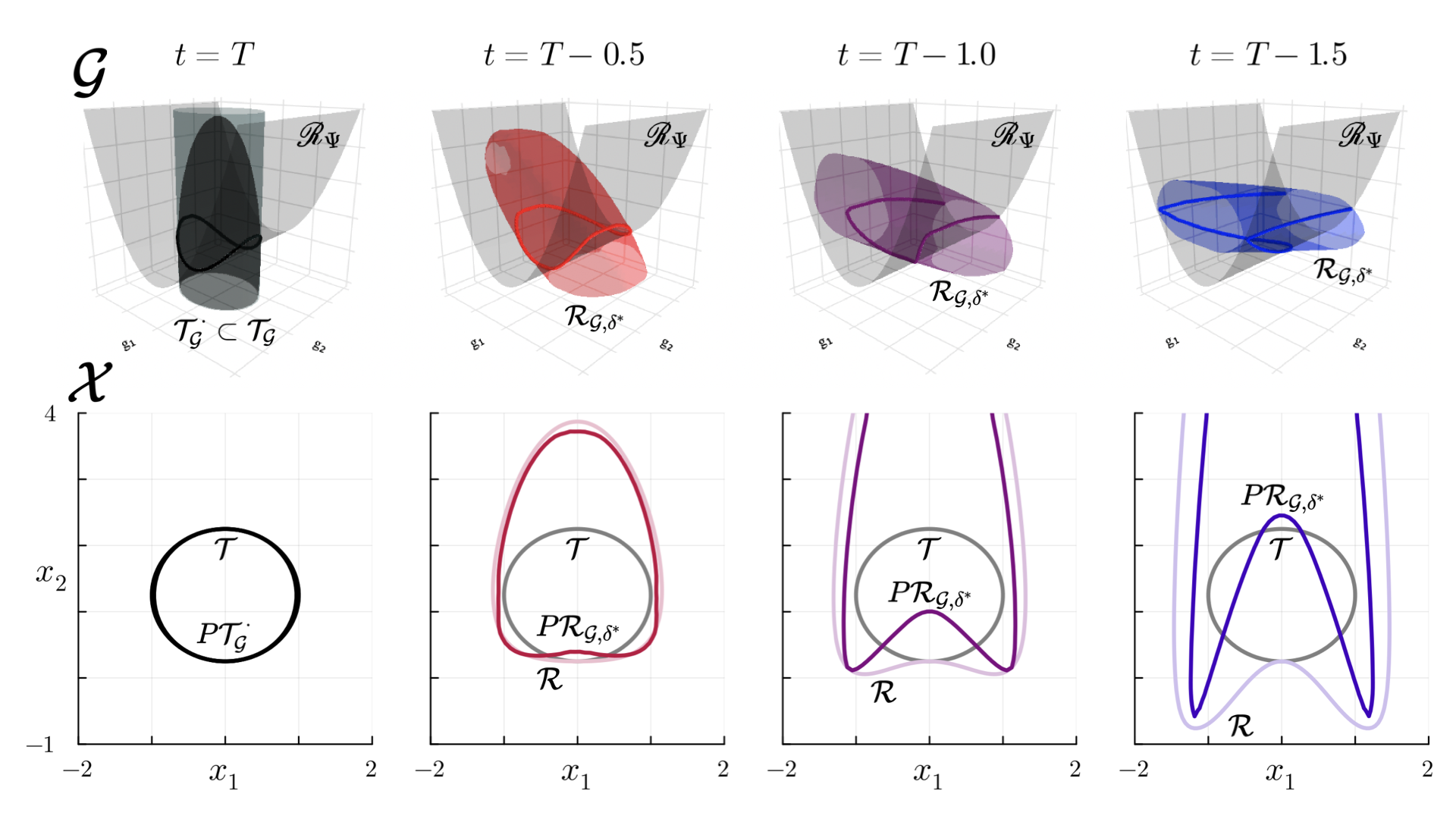
Figure 1: Reach game in the Slow Manifold system (Sec.V-A). The bottom left shows the target $\mathcal{T}\subset\mathcal{X}$. The corresponding augmented target $\mathcal{T}_{\mathcal{G}}\subset\mathcal{G}$, inner augmented target $\mathcal{T}_{\mathcal{G}}^{\cdot}\subset\mathcal{T}_{\mathcal{G}}$ and manifold ${\mathscr{R}}_{\Psi}$ are shown in the top left. The projection of $\mathcal{T}_{\mathcal{G}}^{\cdot}$ restricted to the manifold $P\mathcal{T}_{\mathcal{G}}^{\cdot}\subset\mathcal{T}$ is also shown in the bottom left. The reach set $\mathcal{R}_{\mathcal{G},\delta^{*}}(\mathcal{T}_{\mathcal{G}}^{\cdot},t)$ of the SA linear game with antagonistic error is shown in the top row for different time horizons $t$ (colored transparent sets), and its projection restricted to the manifold $P\mathcal{R}_{\mathcal{G},\delta^{*}}(\mathcal{T}_{\mathcal{G}}^{\cdot},t)$ is shown in the bottom row (dark-colored lines). By Theorem 2, $P\mathcal{R}_{\mathcal{G},\delta^{*}}(\mathcal{T}_{\mathcal{G}}^{\cdot},t)\subset\mathcal{R}$, the reach set $\mathcal{R}$ of the nonlinear game (light-colored lines).

Proof.

First, with the compactness of $\mathcal{T}_{\mathcal{G}}^{\cdot},\mathcal{T}_{\mathcal{G}}^{\circ},\mathcal{U},\mathcal{D}$ and the Lipschitz nature of $\kappa+\varepsilon$, the assumptions (2.1)-(2.4) of [25] are satisfied and $V_{\mathcal{G},\delta^{*}}$ and $V_{\mathcal{G},\delta^{*}}^{-}$ defined in (30) are the viscosity solutions of the HJ-PDEs given in (20) by Theorem  1 [25]. The proof of the Reach game is akin to that of the Avoid game, hence we present only the former case.

Let $g\in{\mathscr{R}}_{\Psi|_{\bar{\mathcal{S}}(\mathcal{T},t)}}$ then $g=\Psi(x),Pg=x$. Assume,

$$V_{\mathcal{G},\delta^{*}}(g,t;\kappa+\varepsilon,\mathcal{T}_{\mathcal{G}}^{\cdot})\leq 0.$$

Then by Corollary  1, Lemma  3, and Lemma  2,

$$\begin{aligned} \implies V_{\mathcal{G},\delta^{*}}(g,t;f_{\mathcal{G}},\mathcal{T}_{\mathcal{G}}^{\cdot})&\leq 0\\ \implies V_{\mathcal{G}}(g,t;f_{\mathcal{G}},\mathcal{T}_{\mathcal{G}})&\leq 0\\ \implies V(x,t;f,\mathcal{T})&\leq 0,\end{aligned}$$

which proves the claim for this case. For $P\mathcal{R}_{\mathcal{G}}\triangleq\{Pg\mid g\in\mathcal{R}_{\mathcal{G}}\cap{\mathscr{R}}_{\Psi}\}$, this is equivalent to saying,

$$P\mathcal{R}_{\mathcal{G},\delta^{*}}(\mathcal{T}_{\mathcal{G}}^{\cdot},t)\subseteq P\mathcal{R}_{\mathcal{G}}(\mathcal{T}_{\mathcal{G}}^{\cdot},t)\subseteq P\mathcal{R}_{\mathcal{G}}(\mathcal{T}_{\mathcal{G}},t)=\mathcal{R}(\mathcal{T},t).$$

Lastly, if $\forall\mathfrak{e}\in\mathfrak{E}(t),\forall\mathfrak{d}\in\mathfrak{D}(t),\exists u_{\mathcal{G},\delta^{*}}^{*}(\cdot)\in\mathbb{U}(t)$ s.t.

$$J_{\mathcal{G}}^{\cdot}(\xi_{\kappa+\varepsilon}(T;g,u_{\mathcal{G},\delta^{*}}^{*}(\cdot),\mathfrak{d}[u_{\mathcal{G},\delta^{*}}^{*}](\cdot),\mathfrak{e}[u_{\mathcal{G},\delta^{*}}^{*}](\cdot),t))\leq 0$$

by the same logical sequence as above,

$$\begin{aligned} \implies\exists\mathfrak{e},\mathfrak{e}[u_{\mathcal{G},\delta^{*}}^{*}]=\varepsilon(\cdot)\text{ s.t. }\\ J_{\mathcal{G}}^{\cdot}(\xi_{f_{\mathcal{G}}}(T;g,u_{\mathcal{G},\delta^{*}}^{*}(\cdot),\mathfrak{d}[u_{\mathcal{G},\delta^{*}}^{*}](\cdot),t)&\leq 0\\ \implies J_{\mathcal{G}}(\xi_{f_{\mathcal{G}}}(T;g,u_{\mathcal{G},\delta^{*}}^{*}(\cdot),\mathfrak{d}[u_{\mathcal{G},\delta^{*}}^{*}](\cdot),t)&\leq 0\\ \implies J(P\xi_{f_{\mathcal{G}}}(T;g,u_{\mathcal{G},\delta^{*}}^{*}(\cdot),\mathfrak{d}[u_{\mathcal{G},\delta^{*}}^{*}](\cdot),t)&\leq 0\\ \implies J(\xi_{f}(T;g,u_{\mathcal{G},\delta^{*}}^{*}(\cdot),\mathfrak{d}[u_{\mathcal{G},\delta^{*}}^{*}](\cdot),t)&\leq 0.\end{aligned}$$

Hence, the control signal $u_{\mathcal{G},\delta^{*}}^{*}(\cdot)$, which may be solved from the linear program in (13) with $L_{1}$ & $V_{\mathcal{G},\delta^{*}}$ (given by the optimal argument of the Hopf formula), will drive the true trajectory into the target despite any disturbance. ∎

V DEMONSTRATION

V-A Slow Manifold System

To illustrate Theorem 2, consider the well-known “slow-manifold” system [17, 35] with inputs,

$$\dot{x}=\begin{bmatrix}\mu x_{1}\\ \lambda(x_{2}-x_{1}^{2})\end{bmatrix}+u+d,$$ (32)

with $\mu,\lambda:=-0.05,-1$, control $u\in\mathcal{U}$ and disturbance $d\in\mathcal{D}$. In the autonomous case, this system has an exact linear representation in the state augmented space defined by $g=\Psi(x)\triangleq[x_{1},x_{2},x_{1}^{2}]^{\top}$ with range $\mathscr{R}_{\Psi}$ given by the quadratic $g_{3}=g_{1}^{2}$. With this lift, the exact SA dynamics $f_{\mathcal{G}}$ are given by,

$$\dot{g}=f_{\mathcal{G}}(g,u,d)=\begin{bmatrix}\mu&0&0\\ 0&\lambda&-\lambda\\ 0&0&2\mu\end{bmatrix}g+\begin{bmatrix}1&0\\ 0&1\\ 2g_{1}&0\end{bmatrix}(u+d).$$ (33)

Of course, when $u$ and $d$ are nontrivial, the presence of $g_{1}$ in the affine term makes $f_{\mathcal{G}}$ nonlinear.

Consider a game governed by the dynamics (32) in which the controller aims to drive the trajectory from an initial $(x,t)$ such that at time $T$ the trajectory is in $\mathcal{T}\triangleq\{y\in\mathcal{X}\mid(y-c_{\mathcal{T}})^{\top}(y-c_{\mathcal{T}})\leq 1\}$ centered at $c_{\mathcal{T}}\triangleq[0,1.25]$, while the disturbance aims to do the opposite (Reach game). Let control and disturbance sets be given by $\mathcal{U}\triangleq\{\|u\|_{2}\leq 1/2\}$ and $\mathcal{D}\triangleq\{\|d\|_{2}\leq 1/4\}$. Choose $\mathcal{T}_{\mathcal{G}}^{\cdot}\triangleq\{(g-\Psi(c_{\mathcal{T}}))^{\top}Q(g-\Psi(c_{\mathcal{T}}))\leq 1\}$ with $Q=\text{Diag}([1,1,\eta])$, where $\eta=1/15$. Since $\eta>0$, then $\mathcal{T}_{\mathcal{G}}^{\cdot}\subset\mathcal{T}_{\mathcal{G}}$. Let the linear model $\kappa$ be defined as in (33) with $g_{1}=\Psi(c_{\mathcal{T}})_{1}=0$ in the input-affine term. The tube $\bar{\mathcal{S}}(\mathcal{T},t)$ is conservatively solved (via [36]) and on a grid over $\bar{\mathcal{S}}(\mathcal{T},t)$ that has been mapped to ${\mathscr{R}}_{\Psi}$, the maximum error $\delta^{*}_{\mathcal{G}}\triangleq\delta^{*}({\mathscr{R}}_{\Psi|_{\bar{\mathcal{S}}(\mathcal{T},t)}})$ is approximated.

The reachable sets $\mathcal{R}(\mathcal{T},t)$ of the true value $V(x,t)$ are shown for different time horizons by the light-colored lines in the bottom row of Figure 1; these are solved with DP (via [37]) over a grid of $100^{2}$ points in $\mathcal{X}$. With the same grid mapped to ${\mathscr{R}}_{\Psi}$ in $\mathcal{X}$, the reachable sets on ${\mathscr{R}}_{\Psi}$ of the SA linear value with antagonistic error $P\mathcal{R}_{\mathcal{G},\delta^{*}}(\mathcal{T}_{\mathcal{G}}^{\cdot},t)$ are solved with the Hopf formula in parallel (via [38]) and also plotted in bottom row of Figure 1 by the dark-colored lines. As shown, these sets are conservative under-approximations of the true reachable sets. Note, unlike DP, the Hopf formula may solve the value at these points without gridding the entire space of $\mathcal{G}$ (or without any grid at all) and in parallel since the value at each point is independent. Solely to elucidate the results, however, on a $100^{3}$ grid in $\mathcal{G}$, the entire reachable set of the SA linear value with antagonistic error $\mathcal{R}_{\mathcal{G},\delta^{*}}(\mathcal{T}_{\mathcal{G}}^{\cdot},t)$ is solved with the Hopf formula (in parallel) and plotted in the top row of Figure 1 with a contour highlighting the intersection of $\mathcal{R}_{\mathcal{G},\delta^{*}}(\mathcal{T}_{\mathcal{G}}^{\cdot},t)$ and ${\mathscr{R}}_{\Psi}$.

V-B Van der Pol System

To observe the results applied to various lifting functions, consider the Van der Pol system with control,

$$\dot{x}=\begin{bmatrix}x_{1}\\ \mu(1-x_{1}^{2})x_{2}-x_{1}\end{bmatrix}+\begin{bmatrix}0\\ 1\end{bmatrix}u$$ (34)

with $\mu=1$ and $u\in\mathcal{U}\triangleq\{|u|\leq 1/2\}$. Let the game in this setting be such that the control aims to drive trajectories away from $\mathcal{T}\triangleq\{x^{\top}x\leq 1\}$ at time $T$ (Avoid game). There is no disturbance in this game i.e. it is an optimal control problem that will, via our method, be converted into a game in the SA space to account for the error of any SA linear model.

Consider state augmentations of this system defined by lifting functions of polynomials of degrees three ($n_{k}=10$) and four ($n_{k}=15$), and radial basis functions (RBFs) with Gaussian kernels with five ($n_{k}=7$) and nine centers ($n_{k}=11$). The linear models for the SA systems are generated by a standard EDMD method which uses the $L_{2}$ error for fitting a linear model to a random trajectory sample of 2k points (via [39]). For all lifting functions, let $\mathcal{T}_{\mathcal{G}}^{\circ}\triangleq\{g^{\top}Qg\leq 10/9\}$ with $Q=\text{Diag}([1,1,\eta\bm{1}])$ with $\bm{1}\in\mathbb{R}^{{n_{k}}-{n_{x}}}$ and $\eta=10$, defining $(\mathcal{T}_{\mathcal{G}}^{\circ}\cap{\mathscr{R}}_{\Psi})\supset(\mathcal{T}_{\mathcal{G}}\cap{\mathscr{R}}_{\Psi})$.

In the same manner as in Sec.V-A, the tube $\bar{\mathcal{S}}(\mathcal{T},t)$ is conservatively solved via [36], the maximum error $\delta^{*}_{\mathcal{G}}\triangleq\delta^{*}({\mathscr{R}}_{\Psi|_{\bar{\mathcal{S}}(\mathcal{T},t)}})$ is approximated on a grid of $\bar{\mathcal{S}}(\mathcal{T},t)$ mapped to ${\mathscr{R}}_{\Psi}$, and then $\mathcal{R}_{\mathcal{G},\delta^{*}}^{-}$ is solved with the Hopf formula and compared to the DP-based ground truth $\mathcal{R}^{-}$ at $t=T-1$. In addition, the Taylor series (TS) and dynamic mode decomposition (DMD) non-augmented solutions $\mathcal{R}_{\delta^{*}}^{-}$ in $\mathcal{X}$ are solved with the Hopf formula and included for comparison. The solutions are shown in Figure  2.

Interestingly in this example, while the mean error on the evolution of identity states decreases with higher $n_{k}$ (not shown), the maximum error does not, and it can be seen that the highest $n_{k}$ does not give the tightest over-approximation. This is consistent with the asymptotic nature of the limit to the Koopman operator [20, 21, 22]. Moreover, this is affected by the natural tendency of the L₂ metric to scale with increased dimension. This could be improved by SA fitting with the L_∞ metric or the consistency index [19] but we leave this to future work.

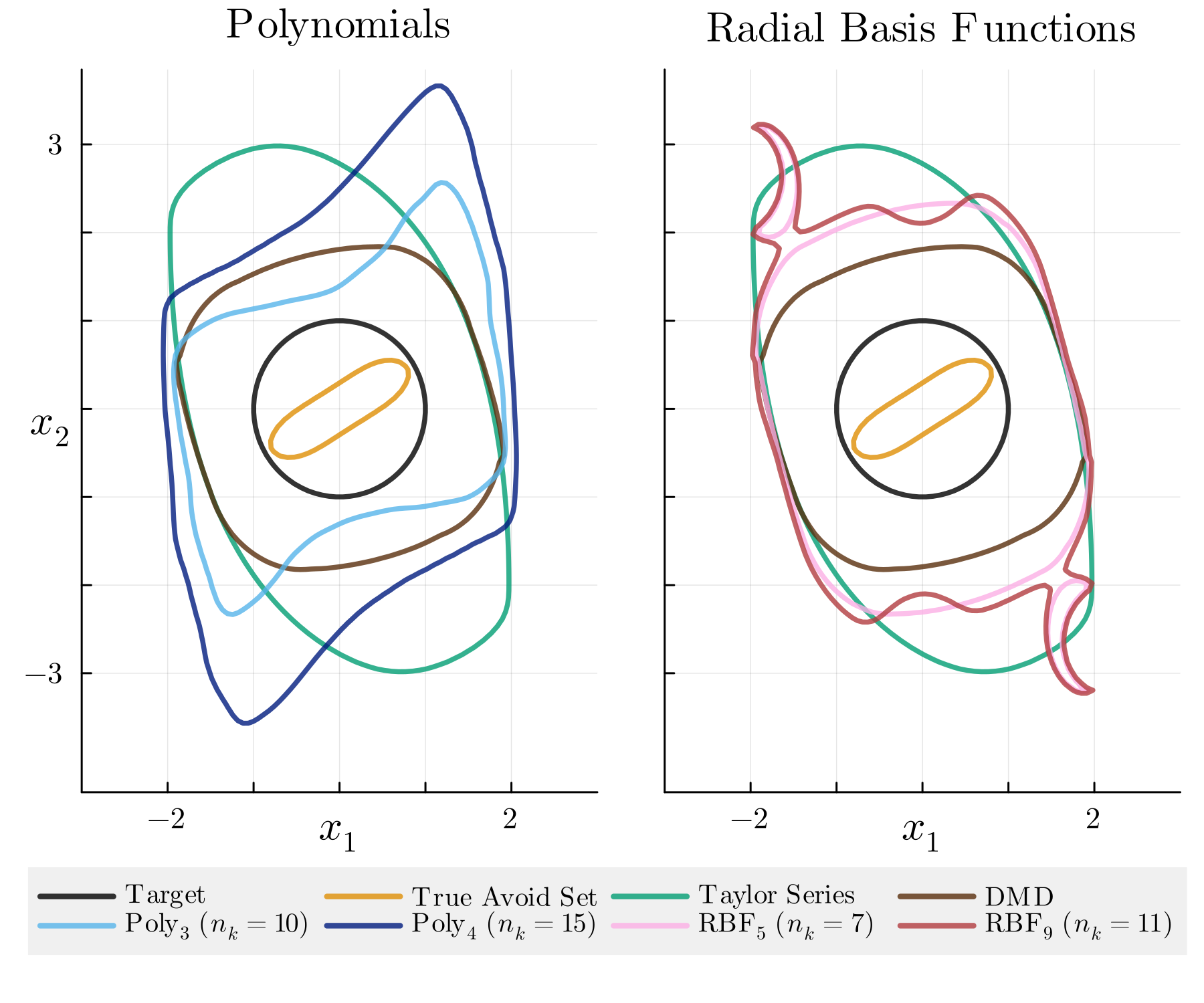
Figure 2: Avoid game in the Van der Pol system (Sec.V-B) with various lifting functions $\Psi$. In both plots, the target $\mathcal{T}$ and the (true) backward avoid set $\mathcal{R}^{-}(\mathcal{T},t)$ are shown in black and gold resp. As baselines, the avoid sets of the games with antagonistic error (without lifting) $\mathcal{R}^{-}_{\delta^{*}}$ with the Taylor Series (TS) and Dynamic Mode Decomposition (DMD) linearizations are shown in green and brown. On the left, the projections restricted to the manifold of the avoid sets of state-augmented linear models with antagonistic error, $P\mathcal{R}^{-}_{\mathcal{G},\delta^{*}}$, are shown for two polynomial lifting functions of degrees three and four respectively in shades of blue. On the right, the $P\mathcal{R}^{-}_{\mathcal{G},\delta^{*}}$ are shown for two RBF lifting functions with five and nine centers respectively in shades of red. Theorem 2 guarantees that for any $\Psi$ satisfying the given assumptions, $P\mathcal{R}^{-}_{\mathcal{G},\delta^{*}}\supset\mathcal{R}^{-}$, therefore the intersection of all $P\mathcal{R}^{-}_{\mathcal{G},\delta^{*}}$ is a valid conservative envelope of the avoid set $\mathcal{R}^{-}(\mathcal{T},t)$. Note, the tightness of the over-approximation depends on the maximum error $\delta^{*}$ for a linear model with any given lifting function.

VI CONCLUSION

In this work, we have devised the construction of a differential game for state-augmented linear models with antagonistic error. Moreover, we prove the corresponding value is conservative with respect to the true value, and by construction, may be used to derive an optimal controller that is guaranteed to succeed in the true dynamics. This is valuable considering that state-augmented systems may have significantly improved accuracy, and the results are amenable to combination (with union or intersection for Reach and Avoid resp.). Moreover, all of the extensions to further reduce the error in [12] are applicable to the current setting and we leave this to future work. Notably, this method also offers a novel way to use linear differential games to approximate solutions in a non-convex fashion. Future work may include extensions to probabilistic error bounds, neural net lifting functions, and non-state inclusive augmented space.

References

- [1] I. M. Mitchell, A. M. Bayen, and C. J. Tomlin, “A time-dependent Hamilton-Jacobi formulation of reachable sets for continuous dynamic games,” IEEE Transactions on automatic control, vol. 50, no. 7, pp. 947–957, 2005.
- [2] S. Bansal, M. Chen, S. Herbert, and C. J. Tomlin, “Hamilton-Jacobi reachability: A brief overview and recent advances,” in 2017 IEEE 56th Annual Conference on Decision and Control (CDC). IEEE, 2017, pp. 2242–2253.
- [3] A. Lin and S. Bansal, “Generating formal safety assurances for high-dimensional reachability,” in 2023 IEEE International Conference on Robotics and Automation (ICRA). IEEE, 2023, pp. 10 525–10 531.
- [4] M. R. Kirchner, R. Mar, G. Hewer, J. Darbon, S. Osher, and Y. T. Chow, “Time-optimal collaborative guidance using the generalized Hopf formula,” IEEE Control Systems Letters, vol. 2, no. 2, pp. 201–206, apr 2018. [Online]. Available: https://doi.org/10.11092Flcsys.2017.2785357
- [5] D. Lee and C. J. Tomlin, “Iterative method using the generalized Hopf formula: Avoiding spatial discretization for computing solutions of Hamilton-Jacobi equations for nonlinear systems,” in 2019 IEEE 58th Conference on Decision and Control (CDC). IEEE, 2019, pp. 1486–1493.
- [6] M. Chen, S. Herbert, and C. J. Tomlin, “Exact and efficient Hamilton-Jacobi guaranteed safety analysis via system decomposition,” in 2017 IEEE International Conference on Robotics and Automation (ICRA). IEEE, 2017, pp. 87–92.
- [7] C. He, Z. Gong, M. Chen, and S. Herbert, “Efficient and guaranteed hamilton-jacobi reachability via self-contained subsystem decomposition and admissible control sets,” IEEE Control Systems Letters, 2023.
- [8] J. Darbon and S. Osher, “Algorithms for overcoming the curse of dimensionality for certain Hamilton–Jacobi equations arising in control theory and elsewhere,” Research in the Mathematical Sciences, vol. 3, no. 1, p. 19, 2016.
- [9] Y. T. Chow, J. Darbon, S. Osher, and W. Yin, “Algorithm for overcoming the curse of dimensionality for time-dependent non-convex Hamilton–Jacobi equations arising from optimal control and differential games problems,” Journal of Scientific Computing, vol. 73, pp. 617–643, 2017.
- [10] ——, “Algorithm for overcoming the curse of dimensionality for state-dependent Hamilton-Jacobi equations,” Journal of Computational Physics, vol. 387, pp. 376–409, 2019.
- [11] W. Sharpless, N. Shinde, M. Kim, Y. T. Chow, and S. Herbert, “Koopman-Hopf Hamilton-Jacobi reachability and control,” arXiv preprint arXiv:2303.11590, 2003.
- [12] W. Sharpless, Y. T. Chow, and S. Herbert, “Conservative linear envelopes for high-dimensional, Hamilton-Jacobi reachability for nonlinear systems via the Hopf formula,” 2024.
- [13] Y. Igarashi, M. Yamakita, J. Ng, and H. H. Asada, “Mpc performances for nonlinear systems using several linearization models,” in 2020 American Control Conference (ACC). IEEE, 2020, pp. 2426–2431.
- [14] M. O. Williams, I. G. Kevrekidis, and C. W. Rowley, “A data–driven approximation of the koopman operator: Extending dynamic mode decomposition,” Journal of Nonlinear Science, vol. 25, pp. 1307–1346, 2015.
- [15] E. Yeung, S. Kundu, and N. Hodas, “Learning deep neural network representations for Koopman operators of nonlinear dynamical systems,” in 2019 American Control Conference (ACC). IEEE, 2019, pp. 4832–4839.
- [16] Y. Li, H. He, J. Wu, D. Katabi, and A. Torralba, “Learning compositional Koopman operators for model-based control,” 2020.
- [17] S. L. Brunton, B. W. Brunton, J. L. Proctor, and J. N. Kutz, “Koopman invariant subspaces and finite linear representations of nonlinear dynamical systems for control,” PloS one, vol. 11, no. 2, p. e0150171, 2016.
- [18] I. Abraham and T. D. Murphey, “Active learning of dynamics for data-driven control using Koopman operators,” IEEE Transactions on Robotics, vol. 35, no. 5, pp. 1071–1083, 2019.
- [19] M. Haseli and J. Cortés, “Modeling nonlinear control systems via koopman control family: Universal forms and subspace invariance proximity,” 2024.
- [20] M. Korda and I. Mezić, “On convergence of extended dynamic mode decomposition to the Koopman operator,” Journal of Nonlinear Science, vol. 28, pp. 687–710, 2018.
- [21] F. Nüske, S. Peitz, F. Philipp, M. Schaller, and K. Worthmann, “Finite-data error bounds for Koopman-based prediction and control,” Journal of Nonlinear Science, vol. 33, no. 1, p. 14, 2023.
- [22] J. J. Bramburger and G. Fantuzzi, “Auxiliary functions as koopman observables: Data-driven polynomial optimization for dynamical systems,” arXiv e-prints, pp. arXiv–2303, 2023.
- [23] B. O. Koopman, “Hamiltonian systems and transformation in Hilbert space,” Proceedings of the National Academy of Sciences, vol. 17, no. 5, pp. 315–318, 1931.
- [24] T. Başar and G. J. Olsder, Dynamic noncooperative game theory. SIAM, 1998.
- [25] L. C. Evans and P. E. Souganidis, “Differential games and representation formulas for solutions of Hamilton-Jacobi-isaacs equations,” Indiana University mathematics journal, vol. 33, no. 5, pp. 773–797, 1984.
- [26] A. F. Filippov, “Differential equations with discontinuous right-hand side,” Matematicheskii sbornik, vol. 93, no. 1, pp. 99–128, 1960.
- [27] J.-P. Aubin and A. Cellina, Differential inclusions: set-valued maps and viability theory. Springer Science & Business Media, 2012, vol. 264.
- [28] J. K. Scott and P. I. Barton, “Bounds on the reachable sets of nonlinear control systems,” Automatica, vol. 49, no. 1, pp. 93–100, 2013.
- [29] A. B. Kurzhanski, “Dynamics and control of trajectory tubes. theory and computation,” in 2014 20th International Workshop on Beam Dynamics and Optimization (BDO). IEEE, 2014, pp. 1–1.
- [30] I. Rublev, “Generalized Hopf formulas for the nonautonomous Hamilton-Jacobi equation,” Computational Mathematics and Modeling, vol. 11, no. 4, pp. 391–400, 2000.
- [31] Y. T. Chow, J. Darbon, S. Osher, and W. Yin, “Algorithm for overcoming the curse of dimensionality for certain non-convex Hamilton–Jacobi equations, projections and differential games,” Annals of Mathematical Sciences and Applications, vol. 3, no. 2, pp. 369–403, 2018.
- [32] D. Bruder, B. Gillespie, C. D. Remy, and R. Vasudevan, “Modeling and control of soft robots using the Koopman operator and model predictive control,” arXiv preprint arXiv:1902.02827, 2019.
- [33] X. Chen, E. Abraham, and S. Sankaranarayanan, “Taylor model flowpipe construction for non-linear hybrid systems,” in 2012 IEEE 33rd Real-Time Systems Symposium. IEEE, 2012, pp. 183–192.
- [34] W. E. Boyce, R. C. DiPrima, and D. B. Meade, Elementary differential equations and boundary value problems. John Wiley & Sons, 2021.
- [35] M. Korda and I. Mezić, “Linear predictors for nonlinear dynamical systems: Koopman operator meets model predictive control,” Automatica, vol. 93, pp. 149–160, 2018.
- [36] S. Bogomolov, M. Forets, G. Frehse, K. Potomkin, and C. Schilling, “JuliaReach: a toolbox for set-based reachability,” in Proceedings of the 22nd ACM International Conference on Hybrid Systems: Computation and Control, 2019, pp. 39–44.
- [37] StanfordASL, “Hamilton-Jacobi reachability analysis in jax.” 2021. [Online]. Available: https://github.com/StanfordASL/hj_reachability
- [38] UCSD-SASLab, “Julia package for Hamilton-Jacobi reachability via Hopf optimization,” 2023. [Online]. Available: https://github.com/UCSD-SASLab/HopfReachability
- [39] S. Pan, E. Kaiser, B. M. de Silva, J. N. Kutz, and S. L. Brunton, “Pykoopman: A python package for data-driven approximation of the Koopman operator,” 2023.