An Optimal Solution to Infinite Horizon Nonlinear Control Problems: Part II

Abstract

This paper considers the infinite horizon optimal control problem for nonlinear systems. Under the condition of nonlinear controllability of the system to any terminal set containing the origin and forward invariance of the terminal set, we establish a regularized solution approach consisting of a “finite free final time” optimal transfer problem to the terminal set which renders the set globally asymptotically stable. Further, we show that the approximations converge to the optimal infinite horizon cost as the size of the terminal set decreases to zero. We also perform the analysis for the discounted problem and show that the terminal set is asymptotically stable only for a subset of the state space and not globally. The theory is empirically evaluated on various nonholonomic robotic systems to show that the cost of our approximate problem converges and the transfer time into the terminal set is dependent on the initial state of the system, necessitating the free final time formulation.

I Introduction

The goal of an optimal control problem is to find the control inputs that minimize a given cost function subject to constraints on the system dynamics. Further, it is desired that the optimal control problem results in a globally asymptotically stable (GAS) closed-loop system. In order to satisfy the GAS requirement, one has to pose an infinite horizon control problem, i.e., where the cost is an infinite sum. This is due to the fact that different initial states typically require different times to reach the desired terminal condition, which is captured by the infinite horizon problem. Although there exists infinite horizon optimal control law for specific, mostly linear, systems, obtaining an optimal solution for an infinite horizon nonlinear control problem is a very challenging task owing to the infinite horizon [1]. In this work, we propose an approximate solution to the infinite horizon optimal control problem by turning the problem into an equivalent finite horizon problem. In particular, we note that if the infinite horizon cost is finite, the tail sum of the cost has to vanish, which implies that the system has to spend most of the infinite time around the origin. Therefore, we use a heuristic terminal cost that can serve as an approximation of the tail cost and pose the problem as a finite horizon problem. Thus, the infinite horizon problem reduces to finding the optimal insertion time, along with the associated control inputs, into a level set of the terminal cost function that contains the origin. As the size of these level sets is decreased, the approximations are shown to converge to the true optimal cost function. Furthermore, although the solution may not be optimal for a finite level set, it nonetheless provides a control Lyapunov function that can globally asymptotically stabilize the underlying system, under a mild nonlinear controllability assumption that any state can be controlled into a terminal set containing the origin, and that the terminal set is forward invariant.

The infinite horizon optimal control problem is typically solved via the stationary Dynamic Programming (DP) problem for discrete-time systems, or the stationary Hamilton-Jacobi-Bellman (HJB) equation in continuous time systems [1, 2]. The optimal solution to the stationary HJB equation is a globally asymptotically stabilizing control Lyapunov function [3, 4, 5]. However, the solution is computationally intractable owing to Bellman’s dreaded “curse of dimensionality” [1, 2]. Thus, there is extensive literature on Approximate DP (ADP) and Reinforcement Learning that seeks to alleviate the curse of dimensionality. ADP methods [6, 7] to give an approximately optimal policy/value function with high confidence. In the past decade, function approximation using deep neural networks has significantly improved the performance of reinforcement learning algorithms, leading to a growing class of literature on ‘deep reinforcement learning’ [8, 9, 10]. Albeit there has been success in solving much higher dimensional problems than previously possible, the inherent variance in the solution [11, 12, 13] renders them unreliable, the training time required of these methods remains prohibitive and it is not possible to assert if the solution is optimal or even characterize its sub-optimality.

An alternative “direct” approach to the HJB is to solve the underlying infinite horizon optimal control problem given a particular initial state. The field of Model Predictive Control (MPC) takes this approach to solve the infinite horizon problem; however, owing to the infinite horizon of the involved optimal control problem, MPC solves a “fixed final time” finite horizon problem in its stead, takes the first control action, and repeats the process at the next state [14, 15]. Most MPC approaches then show the asymptotic stability of the resulting “time invariant” control policy. There are two primary approaches: the first is to use a suitable terminal cost function in the optimization problem that is a control Lyapunov function for the system in some terminal set containing the origin [14]. The domain of attraction of the MPC law under this approach can be undesirably small and different methods have been suggested to increase the domain of attraction [16, 17, 18]. Alternatively, one can eschew the use of a terminal cost function and set using a suitable long horizon and well-designed incremental costs [19, Ch.6], but this typically leads to intractability owing to very long prediction horizons [20]. Additionally, most MPC approaches, like the quasi-infinite horizon approach [21], assume the system is controllable around the origin and gets a linear feedback law to control the system to the origin in the terminal set. In this regard, nonholonomic systems pose a special challenge since their linearization is uncontrollable around the origin or any desired state [22]. Also, the preferred choice of approximating the terminal cost with the cost-to-go of the linear controller is no longer possible. Hence, one has to control the system to the origin or in the neighborhood of the origin using a purely nonlinear controller.

Our approach is analogous to MPC in that we “directly” solve the optimal control problem, but the key difference is that given an initial state, we solve a “free-final time” problem for insertion into a terminal set. We used this approach to address the problem where the system linearization is controllable around the origin in Part I of this paper [23]. In this work, we relax the linear controllability assumption to address the general problem and provide similar guarantees. Further, we address the discounted infinite horizon problem owing to its wide use in the reinforcement learning literature and show similar results as in the undiscounted case. Finally, there is no need for replanning in our approach owing to the free-final time. The primary limitation is that we do not consider state or control constraints in the problem as is typically done in MPC. The primary contribution of this paper is a tractable direct approach for the solution of infinite horizon optimal control problems that is globally asymptotically stabilizing for nonlinear systems under a mild nonlinear controllability assumption into a terminal set containing the origin. We also show that the approximation converges to the optimal infinite horizon cost as the size of the terminal set is reduced to zero. The rest of the paper is organized as follows: we introduce the problem in Section II, the solution approach for the undiscounted problem and the discounted problem are detailed in Section III and IV, respectively, and the method is tested empirically on several nonlinear systems in Section V.

II Problem Formulation

Let us consider the following infinite horizon optimal control problem (IH-OCP):

$$J_{\infty}^{*}(x)=\min_{\{u_{k}\}}\sum_{k=0}^{\infty}c(x_{k},u_{k});~{}~{} \text{given}~{}x_{0}=x$$ (IH-OCP)

$$\text{subject to the dynamics: }x_{k+1} =f(x_{k},u_{k}),$$ (1)

where $x_{k}\in\mathcal{X}\subset\mathbb{R}^{n}$ represents the state of the dynamical system, $u_{k}\in\mathcal{U}\subset\mathbb{R}^{p}$ represents the control input to the dynamical system, and $c(x_{k},u_{k})$ is the incremental cost incurred in taking control action $u_{k}$ at state $x_{k}$. The above problem is an infinite horizon optimal control problem, and thus, solving the problem is, in general, intractable owing to the infinite horizon of the problem. Our goal in this work is to develop a tractable approach to solve the above problem by transforming the problem into a suitable finite horizon problem.

Given that we can obtain a solution to the (IH-OCP), it is well known that the infinite horizon cost-to-go $J^{*}_{\infty}(\cdot)$ satisfies Bellman’s equation [1, Ch.7]:

$$J_{\infty}^{*}(x)=\min_{u}\{c(x,u)+J_{\infty}^{*}(f(x,u))\}.$$ (2)

We restate Corollary 1 from [23] below for the sake of completeness.

Corollary 1

Let $J^{*}_{\infty}(x)$ satisfy the Bellman equation (2), then it is a control Lyapunov function for the system in (1) that renders the origin globally asymptotically stable.

Further, suppose that if there exists a $J_{\infty}(\cdot)$ such that it satisfies the Bellman equation (not necessarily optimal)

$$J_{\infty}(x)=\min_{u}\{c(x,u)+J_{\infty}(f(x,u))\},$$ (3)

then $J_{\infty}(\cdot)$ also is a CLF that renders the origin globally asymptotically stable (GAS).

Thus, another goal for us in solving (IH-OCP) is to construct CLFs as in (2) and (3), such that they render the origin GAS. In this work, we focus on the specific class of systems that are not linearly controllable around the origin, complimentary to the linearly controllable case considered in [23]. Nonholonomic systems fall under this category. Though we cannot guarantee GAS of the origin, we aim to asymptotically stabilize the system into a terminal set.

III Solution to the Infinite Horizon Optimal Control Problem

The cost of IH-OCP can be written as

$$J_{\infty}^{*}(x)=\min_{\{u_{k}\}}\Big{[}\sum_{k=0}^{T-1}c(x_{k},u_{k})+\sum_{k=T}^{\infty}c(x_{k},u_{k})\Big{]},$$

where we choose a $T$ such that the cost-to-go from $x_{T}$ - $J_{\infty}^{*}(x_{T})$ - is very small compared to the cost to transfer from initial state $x$ to $x_{T}$. If one has knowledge of the cost-to-go function $J_{\infty}^{*}(\cdot)$ around the origin, i.e., the cost-to-go of the linearized system, one can pose the IH-OCP as finite horizon problem with $J_{\infty}^{*}(x_{T})$ as an arbitrarily good approximation of the terminal cost. Since we do not have knowledge of the true cost-to-go function as the system linearization is uncontrollable, we instead use a heuristic cost-to-go function $\phi(x)$ and pose the finite horizon problem. Though it is a heuristic, we construct a formulation whose cost converges to the true IH-OCP cost in the limit.

Let us define the finite-horizon optimal control problem (FH-OCP):

$$J^{T}_{\infty}(x) =\min_{\{u_{k}\}}\sum_{k=0}^{T-1}c(x_{k},u_{k})+\phi(x_{T}),$$ (FH-OCP)

subject to: $$~{}x_{k+1}=f(x_{k},u_{k}),~{}\text{and}~{}x_{0}=x,$$

where $\phi(\cdot)$ is a terminal cost function that is continuous and is such that $\phi(x)>0,~{}\forall~{}x\neq 0$, and $\phi(x)=0$ when $x=0$. We shall make the following assumptions for the rest of this section.

Assumption 1

(A1) We assume that the cost function $c(x,u)$ has a global minimum at $(x,u)=(0,0)$, i.e., $\frac{\partial c}{\partial x}\Bigr{|}_{x=0,u=0}=0$ and $\frac{\partial c}{\partial u}\Bigr{|}_{x=0,u=0}=0$, $c(0,0)=0$, and $c(x,u)>0$ $\forall~{}(x,u)\neq(0,0)$.

Assumption 2

(A2) We assume that given any $x\in\mathcal{X}$, and any $\Omega\subset\mathcal{X}$, such that the origin is in $\Omega$, $\exists$ a control sequence $\{\bar{u}_{k}\}_{k=0}^{T(x)-1}$, that ensures $\bar{x}_{T(x)}\in\Omega$ for some $T(x)<\infty$, under the dynamics defined above (1).

Assumption 2 is a controllability assumption that ensures that any state can be controlled into entering the region $\Omega$ in finite time. We use the following definition for the set $\Omega$ in the rest of the paper: $\Omega_{M}=\{x~{}|~{}\phi(x)\leq M\}$.

Assumption 3

(A3) There exists a control policy $\pi(\cdot):\mathcal{X}\rightarrow\mathcal{U}$ that makes the set $\Omega_{M}$ forward invariant under the dynamics in (1), i.e., $f(x,\pi(x))\in\Omega_{M},~{}\forall~{}x\in\Omega_{M}$. Also, let $c(x,\pi(x))\eqcolon c^{\pi}(x)\leq\delta~{}\forall~{}x\in\Omega_{M}.$ Further $c(x,u)>\delta,~{}\forall~{}x\notin\Omega_{M}.$ Here, $\delta$ is a function of $M$, i.e., $\delta=\delta(M)$.

Remark 1

If the system in (1) is linearly controllable around the origin, then the control policy in the set $\Omega$ can be taken as the linear quadratic regulator (LQR) policy, i.e. $\pi(x)=K_{lqr}x$ and the terminal cost can be replaced with the LQR cost-to-go, i.e., $\phi(x)={x}^{\mathsf{T}}Px$, where $P$ is the calculated by solving the algebraic Riccati equation. This case is dealt with in detail in Part I of the paper [23]. In this paper, we consider systems that are not linearly controllable around the origin.

III-A Heuristic Idea

The heuristic idea behind the solution of the infinite horizon optimal control problem is as follows. Let the optimal trajectory be given by $(x_{k}^{*},u_{k}^{*})$ starting at some state $x$. For the optimal cost to be well defined, we need that $\sum_{k=0}^{\infty}c(x_{k}^{*},u_{k}^{*})<\infty$. However, for this infinite sum to be well defined, the tail sum $\sum_{k>T}^{\infty}c(x_{k}^{*},u_{k}^{*})\rightarrow 0$ as $T\rightarrow\infty$. Thus, after some finite time, the cost $\sum_{k>T}^{\infty}c(x_{k}^{*},u_{k}^{*})$ is necessarily small. Given that due to assumption 1 the cost $c(x,u)=0$ only at the origin, it follows that the system spends a very large time around the origin. Thus, the infinite horizon cost may be split into two parts: a “transfer cost” to get the system into the region $\Omega$ and a finite tail cost once within $\Omega$ (see Fig. 1). Since $\Omega$ is forward invariant under the control policy $\pi(\cdot)$ (A3), the system will stay inside $\Omega$. However, in practice, such a policy is usually unknown, and thus, we need a sufficiently small terminal set $\Omega$ such that the uncontrolled system can be considered to be invariant with respect to it. Thus, the basic idea is to turn the infinite horizon problem into a finite horizon problem by approximating the tail sum of the cost by a heuristic terminal cost $\phi(x)$ and find the optimal insertion time $T^{*}(x)$ from state $x$ into the region $\Omega$ along with the associated optimal control. As the region $\Omega$ gets smaller, we get better approximations of the optimal cost function and obtain the optimum in the limit. However, even for a finite $\Omega$, this procedure results in the construction of a CLF that renders the set $\Omega$ globally asymptotically stable. In fact, we can get an uncountable number of such CLFs based on the choice of our incremental cost function $c(x,u)$.

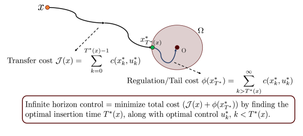
Figure 1: Schematic illustrating the strategy to solve the infinite horizon optimal control problem

III-B Existence of a Finite Horizon Solution

We show below that the solution to (FH-OCP) cannot stay outside $\Omega_{M}$ for infinite time, and there exists a finite time at which the system will enter $\Omega_{M}$.

Lemma 1

There exists a finite time $T(\Omega_{M})<\infty$, such that the solution to (FH-OCP) with $T=T(\Omega_{M})$ denoted by $(\bar{x}_{k},\bar{u}_{k})$ is such that $\phi(\bar{x}_{T(\Omega_{M})})\leq M$ for the first time, i.e., for $T<T(\Omega_{M})$, $\phi(\bar{x}_{k})>M$.

Proof:

We do a proof by contradiction. Let $\{x^{\prime}_{k}\}_{k=0}^{T}$ be the solution to the (FH-OCP). Consider the case where the terminal state $x^{\prime}_{T}$ never enters the set $\Omega_{M}$ for any $T$. Since the cost $c(x,u)\geq\delta>0$ for $x\notin\Omega_{M}$, the cost $J^{T}_{\infty}\rightarrow\infty$ as $T\rightarrow\infty.$

However, owing to A2, there exists a control sequence $\{\bar{u}_{k}\}_{k=0}^{T(x)-1}$ such that $\bar{x}_{T(x)}\in\partial\Omega_{M}$ (boundary of $\Omega_{M}$) for some finite $T(x)$. Let the cost of this trajectory be denoted as

$$\bar{J}(x)=\sum_{k=0}^{T(x)-1}c(\bar{x}_{k},\bar{u}_{k})+M,$$ (4)

where, we have substituted $\phi(\bar{x}_{T(x)})=M$. Choose a $T$ such that $T>T(x)$, and $J^{T}_{\infty}(x)>\bar{J}(x)+\epsilon$, where $\epsilon$ is any positive number. For the sake of the proof we choose $\epsilon=(T-T(x))\delta$, where $\delta$ is as defined in A3, and the reason for this specific choice will be clear below. There is always a $T$ that will satisfy the above requirement since $J^{T}_{\infty}(x)\rightarrow\infty$ as $T\rightarrow\infty.$

Now, apply the policy $\{\bar{u}_{k}\}_{k=0}^{T-1}$ to the system with $\bar{u}_{k}=\pi(\bar{x}_{k})~{}\forall~{}k\geq T(x)$ (recall that $\pi(\cdot)$ is a policy that makes $\Omega_{M}$ invariant and we simply need its existence to prove the result, not know it per se). Let the cost of this trajectory be denoted as $\tilde{J}^{T}_{\infty}(x)$ and is given by $\tilde{J}^{T}_{\infty}(x)=\sum_{k=0}^{T(x)-1}c(\bar{x}_{k},\bar{u}_{k})+\sum_{k=T(x)}^{T-1}c(\bar{x}_{k},\bar{u}_{k})+\phi(\bar{x}_{k})$.

Using A3 and using the fact that $\phi(\bar{x}_{T})<M$ since $\bar{x}_{T}\in\Omega_{M}$, we can write

$$\tilde{J}^{T}_{\infty}(x)\leq\sum_{k=0}^{T(x)-1}c(\bar{x}_{k},\bar{u}_{k})+\underbrace{(T-T(x))\delta}_{=\epsilon}+M.$$ (5)

Substituting (4) in the above inequality, we get, $\tilde{J}^{T}_{\infty}(x)\leq\bar{J}+\epsilon$.

We know, $J^{T}_{\infty}(x)$ is the optimal cost for the (FH-OCP), so $J^{T}_{\infty}(x)\leq\tilde{J}^{T}_{\infty}(x)$, and hence $J^{T}_{\infty}(x)\leq\bar{J}+\epsilon$. This contradicts the fact that we chose $T$ such that $J^{T}_{\infty}(x)>\bar{J}+\epsilon$. Thus, the solution to (FH-OCP) cannot stay outside $\Omega_{M}$ for all $T$, and there exists a finite $T$ such that the solution hits $\Omega_{M}$. ∎

III-C An Alternative Construction

We now define an alternate finite horizon construction to IH-OCP that will use the first hitting time to $\Omega_{M}$ as the time horizon and whose cost will satisfy the Bellman equation. The construction is suboptimal to the IH-OCP, but we show that the cost of this new construction converges to the true IH-OCP cost in the limit $M\rightarrow 0$. We call this the alternate construction optimal control problem (AC-OCP), and it is defined as:

$$J^{M}_{\infty}(x) =\min_{\{u_{k}\}_{k=0}^{T-1},T}\sum_{k=0}^{T-1}c(x_{k},u_{k})+\max(\phi(x_{T}),M)$$ (AC-OCP)

subject to: $$~{}x_{k+1}=f(x_{k},u_{k}),$$

$$x_{T}\in\Omega_{M},~{}\text{and given}~{}x_{0}=x.$$

Note: The above problem has a free final time $T$ that needs to be optimized over in conjunction with the control actions. The free final time will prove crucial to showing the cost function is a CLF and it converges to the optimal IH-OCP cost.

We now prove the following result.

Lemma 2

The optimal time $T^{*}$ to the (AC-OCP) is the first hitting time of the set $\Omega_{M}$ for the (FH-OCP), i.e., $T^{*}=T(\Omega_{M}).$

Proof:

Let the solution to (AC-OCP) be denoted by $(\tilde{x}_{k},\tilde{u}_{k})$ and the cost be given by:

$$J^{M}_{\infty}(x)=\sum_{k=0}^{T^{*}-1}c(\tilde{x}_{k},\tilde{u}_{k})+M.$$ (6)

We consider two cases: $T^{*}>T(\Omega_{M})$ and $T^{*}<T(\Omega_{M}).$
1) $T^{*}>T(\Omega_{M}),~{}\tilde{x}_{T^{*}}\in\Omega_{M}$:
We can say the following from (6):

$$J^{M}_{\infty}(x)>\sum_{k=0}^{T(\Omega_{M})-1}c(\tilde{x}_{k},\tilde{u}_{k})+M,$$ (7)

because $J^{M}_{\infty}(x)$ will have the additional $\sum_{k=T(\Omega_{M})}^{T^{*}-1}c(\tilde{x}_{k},\tilde{u}_{k})$ terms. We also know that optimal cost of (FH-OCP) with horizon $T(\Omega_{M})$ will satisfy

$$J^{T(\Omega_{M})}_{\infty}\leq\sum_{k=0}^{T(\Omega_{M})-1}c(\tilde{x}_{k},\tilde{u}_{k})+M,$$ (8)

because $J^{T(\Omega_{M})}_{\infty}$ is the optimum for the (FH-OCP). From (7) and (8), we can say $J^{M}_{\infty}(x)>J^{T(\Omega_{M})}_{\infty}$, which contradicts the fact that $J^{M}_{\infty}(x)$ is the optimum for (AC-OCP), and hence $T^{*}$ cannot be the optimal time.
2) $T^{*}<T(\Omega_{M}):$
We know $T(\Omega_{M})$ is the first hitting time. Hence for any $T<T(\Omega_{M})$, $\tilde{x}_{T}\notin\Omega_{M}$, which is a constraint the solution to (AC-OCP) has to satisfy. Hence, the optimal time $T^{*}$ cannot be less than $T(\Omega_{M}).$ ∎

The intuition behind the above lemma is that the system incurs more cost when its solution is in the interior of set $\Omega_{M}$ due to the $\max$ function, i.e., $\max(\phi(x_{T}),M)=M$ as $\phi(x_{T})<M$. Hence the optimal solution will be the one that stops at the boundary of set $\Omega_{M}$ when $\phi(x_{T})=M$, which is the solution with time horizon as the first hitting time $T(\Omega_{M}).$

Now, we go on to show that the cost of AC-OCP satisfies the Bellman equation.

Lemma 3

The cost-to-go of AC-OCP $J^{M}_{\infty}(x)$ satisfies the Bellman equation for all initial states $x\notin\Omega_{M}$.

Proof:

The optimal cost of AC-OCP can be written as

$$J^{M}_{\infty}(x) =\min_{\{u_{k}\}_{k=0}^{T-1},T}\Big{[}c(x,u_{0})+\sum_{k=1}^{T-1}c(x_{k},u_{k})$$

$$+\max(\phi(x_{T}),M)\Big{]}.$$

The above equation can also be written as:

$$J^{M}_{\infty}(x) =\min_{u_{0}}\Big{[}c(x,u_{0})+\min_{\{u_{k}\}_{k=1}^{T-1},T}[\sum_{k=1}^{T-1}c(x_{k},u_{k})$$

$$+\max(\phi(x_{T}),M)]\Big{]},$$

$$J^{M}_{\infty}(x) =\min_{u_{0}}\Big{[}c(x,u_{0})+J^{M}_{\infty}(f(x,u_{0}))\Big{]}.$$

The above can be shown for any initial state $x\notin\Omega_{M}$. ∎

Corollary 2

If there exists some $M>0$ such that the set $\Omega_{M}$ is forward invariant for the uncontrolled dynamics or if we have knowledge of a policy $\pi(\cdot)$ that renders the closed loop invariant with respect to $\Omega_{M}$, $J_{\infty}^{M}(\cdot)$ is a CLF for the given system (1), and its policy renders the set $\Omega_{M}$ asymptotically stable.

In the following theorem, we show that the cost of AC-OCP converges to the optimal IH-OCP cost as $M\rightarrow 0.$

Theorem 1

The AC-OCP cost $J^{M}_{\infty}(x)$ converges to the IH-OCP cost $J^{*}_{\infty}(x)$ in the limit $M\rightarrow 0$, i.e.,

$$\lim_{M\rightarrow 0}J^{M}_{\infty}(x)=J^{*}_{\infty}(x),$$

assuming that $J^{*}_{\infty}(\cdot)$ is continuous at the origin.

Proof:

Let $(\tilde{x}_{k},\tilde{u}_{k})$ denote the solution to (AC-OCP), and $(x^{*}_{k},u^{*}_{k})$ denote the solution to (IH-OCP). Now, we compare the costs by applying the AC-OCP policy $\{\tilde{u}_{k}\}_{k=0}^{T(\Omega_{M})}$ to the IH-OCP. Since the AC-OCP policy is only defined for $T(\Omega_{M})$ steps, we assume $\tilde{u}_{k}=u^{*}_{k}$ for $k\geq T(\Omega_{M})$ for the sake of argument, and the result still holds for any policy that renders the set $\Omega_{M}$ forward invariant for the system dynamics. Since $J^{*}_{\infty}(x)$ is the optimal for (IH-OCP), the cost of any other policy satisfies,

$$J^{*}_{\infty}(x)\leq\sum_{k=0}^{T(\Omega_{M})-1}c(\tilde{x}_{k},\tilde{u}_{k})+\sum_{k=T(\Omega_{M})}^{\infty}c(\tilde{x}_{k},u^{*}_{k}).$$ (9)

Using the knowledge that $J^{M}_{\infty}(x)=\sum_{k=0}^{T(\Omega_{M})-1}c(\tilde{x}_{k},\tilde{u}_{k})+M$, and $\sum_{k=T(\Omega_{M})}^{\infty}c(\tilde{x}_{k},u^{*}_{k})=J^{*}_{\infty}(\tilde{x}_{T(\Omega_{M})})$, we can write (9) as,

$$J^{*}_{\infty}(x)\leq J^{M}_{\infty}(x)-M+J^{*}_{\infty}(\tilde{x}_{T(\Omega_{M})}).$$

Restructuring the equation and taking the limit $M\rightarrow 0$ gives,

$$\lim_{M\rightarrow 0}(J^{*}_{\infty}(x)-J^{M}_{\infty}(x))\leq\lim_{M\rightarrow 0}(J^{*}_{\infty}(\tilde{x}_{T(\Omega_{M})})-M),$$

where, $\lim_{M\rightarrow 0}J^{*}_{\infty}(\tilde{x}_{T(\Omega_{M})})=J^{*}_{\infty}(\lim_{M\rightarrow 0}\tilde{x}_{T(\Omega_{M})})$, as $J^{*}_{\infty}(\cdot)$ is continuous at the origin. As $M\rightarrow 0,~{}\Omega_{M}$ will shrink in size and in the limit, $\Omega_{M}=\{0\}$ (since only $x=0$ satisfies the condition $\phi(x)\leq 0,$ and please note the distinction between the number 0 and the state space origin 0.) Hence, in the limit $\tilde{x}_{T(\Omega_{M})}=0$ due to the terminal state constraint $\tilde{x}_{T(\Omega_{M})}\in\Omega_{M}$ in (AC-OCP), which implies $\lim_{M\rightarrow 0}J^{*}_{\infty}(\tilde{x}_{T(\Omega_{M})})=J^{*}_{\infty}(0)=0$. Thus,

$$\lim_{M\rightarrow 0}J^{M}_{\infty}(x)\geq J^{*}_{\infty}(x).$$ (10)

Similarly, we can show $\lim_{M\rightarrow 0}(J^{M}_{\infty}(x)-J^{*}_{\infty}(x))\leq 0$ by applying the IH-OCP policy $\{u^{*}_{k}\}_{k=0}^{\infty}$ to (AC-OCP). Due to the optimality of $J^{M}_{\infty}(x)$, we get $J^{M}_{\infty}(x)\leq\sum_{k=0}^{T(\Omega_{M})-1}c(x^{*}_{k},u^{*}_{k})+\max(\phi(x^{*}_{T(\Omega_{M})},M)=J^{*}_{\infty}(x)-J^{*}_{\infty}(x^{*}_{T(\Omega_{M})})+\max(\phi(x^{*}_{T(\Omega_{M})},M)$. Rearranging and taking the limit gives,

$$\lim_{M\rightarrow 0}\Big{(}J^{M}_{\infty}(x)-J^{*}_{\infty}(x)\Big{)} \leq\lim_{M\rightarrow 0}\Big{(}-J^{*}_{\infty}(x^{*}_{T(\Omega_{M})})$$

$$+\max(\phi(x^{*}_{T(\Omega_{M})},M)\Big{)}$$

As shown previously $\lim_{M\rightarrow 0}J^{*}_{\infty}(x^{*}_{T(\Omega_{M})})=0$. If $\max(\phi(x^{*}_{T(\Omega_{M})},M)=\phi(x^{*}_{T(\Omega_{M})})$, then $\lim_{M\rightarrow 0}\phi(x^{*}_{T(\Omega_{M})})=\phi(\lim_{M\rightarrow 0}x^{*}_{T(\Omega_{M})})$, since $\phi(\cdot)$ is also a continuous function. Using the similar argument used for $J^{*}_{\infty}(\cdot),$ we can say $\phi(\lim_{M\rightarrow 0}x^{*}_{T(\Omega_{M})})=0$. If $\max(\phi(x^{*}_{T(\Omega_{M})},M)=M$, it is trivial to show the limit is $0$. Hence, we get

$$\lim_{M\rightarrow 0}J^{M}_{\infty}(x) \leq J^{*}_{\infty}(x).$$ (11)

From (10) and (11), we get $\lim_{M\rightarrow 0}J^{M}_{\infty}(x)=J^{*}_{\infty}(x).$ ∎

The intuition for the above proof is that as $M\rightarrow 0$, the set $\Omega_{M}$ shrinks in size and the state at the first hitting time $x_{T(\Omega_{M})}\rightarrow 0$, in which case, the AC-OCP and IH-OCP become equivalent problems.

III-D Discussion

Why propose the AC-OCP?

The purpose of proposing the AC-OCP is that it captures the essence of the IH-OCP in that the problem determines the transfer time, for which it has to be free, as opposed to fixed, as in FH-OCP. Moreover, the transfer time is not unique; it varies with the initial state in that different initial states would need different transfer times for optimal performance. Also, the AC-OCP construction helps us guarantee that the finite optimal time cost-to-go is a CLF that renders the set $\Omega_{M}$ globally asymptotically stable.

How would one solve the AC-OCP?

We do not solve AC-OCP directly. The solution is given by solving (FH-OCP) by sweeping for different values of the time horizon $T$ until we find the time $T^{*}$, for which the solution enters the set $\Omega_{M}$, i.e., the terminal cost of the solution satisfies $\phi(x_{T})\leq M$. This sweep of different values of $T$ can be done in parallel, and the search can be optimized to find the $T^{*}.$

How is this different from [23]?

In [23], the stationary optimal cost function, obtained by solving the stationary Riccati equation, was the obvious candidate for the terminal cost since it is an arbitrarily good approximation of the true optimal cost as the terminal set gets small. In lieu, in this work, because of the absence of linear controllability, we use the heuristic terminal cost $\phi(\cdot)$ which only has the property that $\phi(x)\rightarrow 0$ as $x\rightarrow 0$. The advantage in the linearly controllable case is that the terminal set for which the linear controller is a CLF/ good approximation can be quite large, thereby leading to a significant computational saving in solving the problem when compared to solving it without the terminal cost. As we shall show in our computational experiments, the heuristic terminal cost regularization is necessary to solve complex nonholonomic problems such as the fish and swimmer models.

Contrast with Nonlinear MPC

Traditional nonlinear MPC has a fixed horizon $N$, and it replans over the same fixed horizon at every step to furnish a time-invariant control law [15]. This has the implication that the MPC policy only renders states that can be controlled to the terminal set in at most $N$ steps asymptotically stable, leading to a small region of attraction. In contrast, we solve the problem from any initial state over a free horizon and this is precisely what allows for the GAS nature of the resulting policy. Further, this obviates the need for replanning in our approach.

IV Solution to the Discounted Infinite Horizon Optimal Control Problem

Reinforcement learning problems for continuous control predominantly consider discounted infinite horizon problems [24]. In this section, we explore the discounted problem and show that we can use a finite horizon construction similar to the previous section. The discounted problem [25] is defined as

$$J^{*}_{\infty}(x) =\min_{u_{k}}\sum_{k=0}^{\infty}\beta^{k}c(x_{k},u_{k}),$$ (D-IHOCP)

$$\text{subject to:}~{}x_{k+1}=f(x_{k},u_{k}),~{}\text{and}~{}x_{0}=x,$$

where discount factor $\beta\in(0,1)$.

Similar to Section III, we use an alternate construction with a free final time for the discounted finite horizon optimal control problem:

$$J_{\infty}^{M}(x) =\min_{u_{k},T}\sum_{k=0}^{T-1}\beta^{k}c(x_{k},u_{k})+\beta^{T}\max(\phi(x_{k}),M),$$ (D-ACOCP)

$$\text{subject to:}~{}x_{k+1}=f(x_{k},u_{k}).$$

where $\phi(\cdot)$ is some terminal cost function, $\Omega_{M}=\{x:\phi(x)\leq M\}$ and $M<\infty$ is some number.

We invoke assumptions A1, A2, and A3 as established in Section III for the results below. We will prove results for the discounted problem analogous to the undiscounted case. First, we will show that given any initial set $\Omega^{0}$, there always exists a $\beta<1$ such that any $x_{0}\in\Omega^{0}$ may be controlled into the terminal set $\Omega_{M}$ (see Fig. 2).

Figure 2: An illustration of the discounted cost problem. We will show that given any $\Omega^{0}$, there exists a $\beta<1$, s.t., any $x_{0}\in\Omega^{0}$ may be controlled into the terminal set $\Omega_{M}$.

Lemma 4

Given any $x_{0}\in\Omega^{0}$, there exists a discount factor $\beta(x_{0})<1$ such that, given sufficient time, the solution to (D-ACOCP) will enter the set $\Omega_{M}$.

Proof:

We drop the explicit dependence on $x_{0}$ in the following for convenience. We do the proof by contradiction. Recall from A2; there exists a control sequence $\{\bar{u}_{k}\}_{k=0}^{T(x)-1}$ which enters $\Omega_{M}$ at some finite time $T(x)$. Let $T(x)=\bar{T}$ for the given initial state $x$. The trajectory is denoted by $(\bar{x}_{k},\bar{u}_{k})$, and let $\bar{J}$ be the cost associated with it, assuming that the policy $\pi(\cdot)$ is applied once the trajectory enters $\Omega_{M}$. Note that since $c^{\pi}(x)<\delta$, the tail cost is finite, i.e., $\sum_{k>\bar{T}}^{\infty}c^{\pi}(\bar{x}_{k})\beta^{k}<\infty$.

Suppose that the solution to (D-ACOCP) never enters $\Omega_{M}$. Then, the cost of the policy from $\bar{T}$ till some $T>\bar{T}$ is $\sum_{k=\bar{T}}^{T}\beta^{k}c(x_{k},u_{k})=\beta^{\bar{T}}\sum_{k=0}^{T-\bar{T}}\beta^{k}c(x_{k+\bar{T}},u_{k+\bar{T}})\geq\beta^{\bar{T}}\sum_{k=0}^{T-\bar{T}}\beta^{k}\delta=\beta^{\bar{T}}\Bigg{(}\frac{1-\beta^{(T-\bar{T})}}{1-\beta}\Bigg{)}\delta.$

We now show that it is always possible to find a $\beta,T$ such that $\beta^{\bar{T}}\Big{(}\frac{1-\beta^{(T-\bar{T})}}{1-\beta}\Big{)}\delta>\bar{J}+\beta^{T}M$.

The above implies that: $\Bigg{(}\frac{1-\beta^{(T-\bar{T})}}{1-\beta}\Bigg{)}>\frac{\bar{J}+\beta^{T}M}{\delta\beta^{\bar{T}}}$, for some $(\beta,T)$. Now, consider the function $f(\beta,T)=\frac{1-\beta^{(T-\bar{T})}}{1-\beta}$.This function is continuous in $(\beta,T)$, and $\lim_{T\rightarrow\infty,\beta\rightarrow 1}f(\beta,T)\rightarrow\infty$. By definition, this implies that $\exists~{}(\beta,T)$ s.t. $f(\beta,T)>\frac{\bar{J}+\beta^{T}M}{\delta\beta^{\bar{T}}}$. However, this implies that the (D-ACOCP) optimal cost corresponding to the time $T$, say $J_{\infty}^{M,T}>\bar{J}+\beta^{T}M$, thereby contradicting the fact that $J_{\infty}^{M,T}$ is optimum. Note that $(\bar{J}+\beta^{T}M)$ is an upper bound on the cost of the nominal policy $\bar{u}_{k}$ with the terminal policy $\pi(\cdot)$. Thereby, this implies that the solution to the (D-ACOCP) has to enter $\Omega_{M}$ for some finite time, given $\beta$ is sufficiently close to $1$. ∎

We assume the following to remove the dependence on $x_{0}$ for $\beta$.

Assumption 4

Let $\sup\limits_{x_{0}\in\Omega^{0}}\bar{T}(x_{0})<\bar{T}<\infty$, and let $\sup\limits_{x_{0}\in\Omega^{0}}\bar{J}(x_{0})<\bar{J}<\infty$.

Then, if we choose $\beta,T$ s.t. $\Big{(}\frac{1-\beta^{(T-\bar{T})}}{1-\beta}\Big{)}>\frac{\bar{J}+\beta^{T}M}{\delta\beta^{\bar{T}}}$, then the solution to (D-ACOCP) hits the set $\Omega_{M}$ in finite time for any $x_{0}\in\Omega^{0}$.

Corollary 3

Under Assumption 4, $\exists$ a finite $\beta<1$ s.t. the solution to the (D-ACOCP) enters $\Omega_{M}$ in finite time.

Now, we will show that the solution to (D-ACOCP) gives the first hitting time of the set $\Omega_{M}$.

Lemma 5

The optimal time $T^{*}$ for the (D-ACOCP) is the first hitting time of the set $\Omega_{M}$, i.e., $T^{*}=T(\Omega_{M})$.

Proof:

The proof is identical to the proof of Lemma 2. ∎

Now, we show that the cost-to-go of the alternate construction will satisfy the discounted Bellman equation.

Lemma 6

The cost-to-go of (D-ACOCP) $J_{\infty}^{M}(x)$ satisfies the discounted Bellman equation for all initial states $x\notin\Omega_{M}$.

Proof:

The optimal cost of (D-ACOCP) can be written as

$$J^{M}_{\infty}(x) =\min_{\{u_{k}\}_{k=0}^{T-1},T}\Big{[}\beta^{0}c(x,u_{0})+\sum_{k=1}^{T-1}\beta^{k}c(x_{k},u_{k})$$

$$+\beta^{T}\max(\phi(x_{T}),M)\Big{]}.$$

The above equation can also be written as:

$$J^{M}_{\infty}(x) =\min_{u_{0}}\Big{[}c(x,u_{0})+\min_{\{u_{k}\}_{k=1}^{T-1},T}\beta[\sum_{k=1}^{T-1}\beta^{k-1}c(x_{k},u_{k})$$

$$+\beta^{T-1}\max(\phi(x_{T}),M)]\Big{]},$$

$$J^{M}_{\infty}(x) =\min_{u_{0}}\Big{[}c(x,u_{0})+\beta J^{M}_{\infty}(f(x,u_{0}))\Big{]}.$$

The above can be shown for any initial state $x\notin\Omega_{M}$ and time step $k$. ∎

Remark 2

Note that $\beta<1$ only for some $\Omega^{0}\subset\mathcal{X}$, and thus, the discounted policy cannot be globally asymptotically stable.

Finally, we will show that the cost-to-go of the alternate discounted problem converges to the optimum cost of D-IHOCP.

Theorem 2

The D-ACOCP cost $J^{M}_{\infty}(x)$ converges to the discounted infinite-horizon OCP cost $J^{*}_{\infty}(x)$ in the limit $M\rightarrow 0$, i.e.,

$$\lim_{M\rightarrow 0}J^{M}_{\infty}(x)\rightarrow J^{*}_{\infty}(x).$$

Proof:

The proof is essentially identical to the undiscounted case discussed in Theorem 1. ∎

Remark 3

Note that finding the right $\beta$ given some set $\Omega^{0}$ is practically infeasible, as the requisite $\bar{T}$, $\bar{J}$ etc., are unknown in general. Thus, the above result is strictly an existence result, and has no practical way of implementation. In practice, the process is reversed: we choose a $\beta$ and such a choice may have a small region of attraction $\Omega^{0}$ resulting in policies that are myopic.

V Empirical Results

In this section, we present the empirical results. The proposed theory is extended to a Car-like robot (4 states, 2 inputs) and the MuJoCo-based simulators for the 3-link Swimmer (8 states, 2 inputs) and the Fish-robot (27 states, 6 inputs). We show that the cost converges as the horizon or the transfer time is increased. We also show the dependence of the transfer time on the initial conditions. We only show experiments for the undiscounted case here due to paucity of space.

V-A System Description

The Car-like robot has well-established nonlinear dynamics, and is simulated in MATLAB, using an RK4-based solver forward propagation of the model. Given an initial condition $x_{0}=(0,0,\pi/3,0)$, the task is drive the system to $x_{T}=(1,4,\pi/2,0)$. We define the Swimmer optimal control task to start from rest at the origin and reach the target state for its head at coordinates $(0.5,-0.6)$ within finite time. Similarly, the Fish-robot also starts at the origin, with the target coordinates for its head at $(0.4,0.2,1)$. The initial and final states of the models can be observed in Fig. 3. All these systems are nonholonomic, and thus, the terminal cost cannot be the cost-to-go of the linearized system as proposed in our previous work [23].

(a)

(b)

(c)

(d)

Figure 3: Models simulated in MuJoCo in their initial and final states.

(a) Total cost - Car-like robot

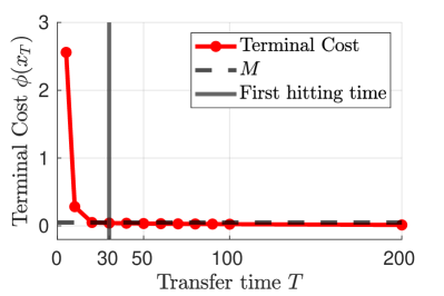
(b) Terminal cost - Car-like robot

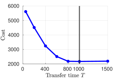
(c) Total cost - 3-link Swimmer

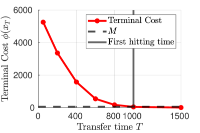
(d) Terminal cost - 3-link Swimmer

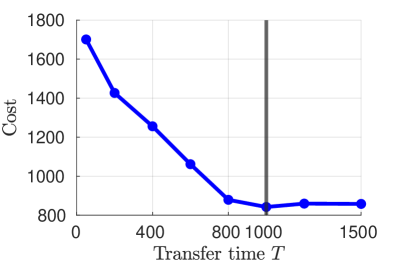
(e) Total cost - Fish-robot

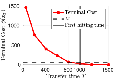
(f) Terminal cost - Fish-robot

Figure 4: Results for the car-like robot, and the MuJoCo-based 3-link Swimmer and Fish robots. Observe that as we increase $T$ beyond the first hitting point $T(\Omega_{M})$, the total finite-horizon cost has essentially converged.

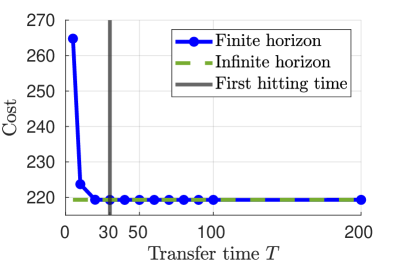
(a) Car-like - Total cost - Case 1

(b) Car-like - Terminal cost - Case 1

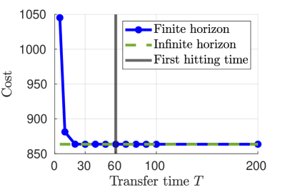
(c) Car-like - Total cost - Case 2

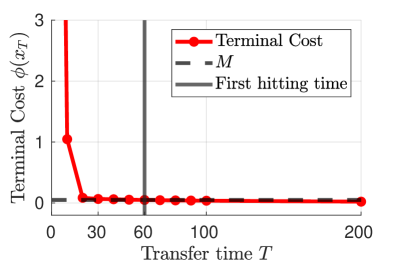
(d) Car-like - Terminal cost - Case 2

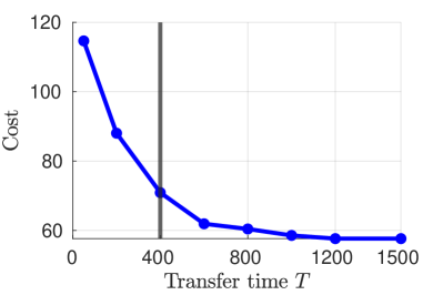
(e) Fish - Total cost - Case 1

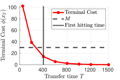
(f) Fish - Terminal cost - Case 1

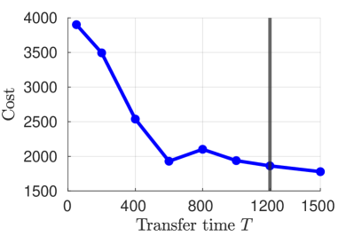
(g) Fish - Total cost - Case 2

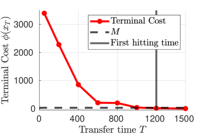
(h) Fish - Terminal cost - Case 2

Figure 5: Results for the car-like robot (a)-(d), and the fish model (e)-(h) with two different initial conditions - labeled Case 1 and 2. Here, we consider $M=0.05$ for the car-like robot, and $M=30$ for the Fish-robot. It is observed that different initial conditions correspond to different transfer times in both cases.

V-B Simulations

To empirically verify our proposed approach, we need to show that the cost of the AC-OCP converges to the infinite horizon optimal cost. We use the iterative Linear Quadratic Regulator (iLQR) algorithm [26] to solve for the nonlinear optimal control and its corresponding optimal cost. For smooth nonlinear systems with control affine dynamics and a quadratic control cost, it can be shown that the iLQR algorithm will converge to the unique global optimum [13] for a sufficiently small time discretization, thus circumventing the issue of multiple local minima.

The ILQR incremental cost parameters and the terminal cost $\phi(x_{T})$ are suitably chosen, and the optimization problem is set up with a finite horizon or ‘transfer time’ $T$. Next, we sweep the transfer time $T$, until and beyond the first-hitting time $T(\Omega_{M})$, where $x_{T(\Omega_{M})}\in\Omega_{M}$. A small value is chosen for $M$, such that the terminal cost is arbitrarily close to zero, i.e. the system is very close to the target state, and thus, the set $\Omega_{M}$ is forward invariant for all practical purposes. Since we do not have the solution for the IH-OCP, the infinite-horizon optimal cost is computed by taking a long enough horizon for each problem without the terminal cost and using ILQR to solve the optimization. The infinite horizon cost for the car-like robot was calculated with a horizon of $1000$. The fish and swimmer models fail to converge without a terminal cost, so we do not plot the infinite horizon cost for those systems. This is another reason to have a regularizing terminal cost for complex systems for stability, in addition to the free final time. It is observed that for any $T>T(\Omega_{M})$, the cost $J^{T}_{\infty}(x)$ converges to the true optimal cost of the IH-OCP for the car-like robot, while still converging to the forward-invariant set for the more complex cases. (Fig. 4). It is also observed that, for smaller horizons less than the first hitting time, the terminal cost remains high, and correspondingly the system fails to converge to the target state. The experiments, thus, empirically validate Lemma 2, wherein increasing the horizon past the first hitting time does not lead to a significant decrease in the cost, and hence, the first hitting time is sufficient to reach the goal set.

In order to observe the dependence of the transfer time on the initial state, the above experiment is repeated for different initial conditions for the Fish and Car-like robot systems. The initial and target states for the corresponding cases are tabulated in Table I. We observe clearly that the hitting time $T(\Omega_{M})$ depends on the initial condition of the system (Fig. 5).

System	Case #	Initial state	Terminal state	$M$
Car-like	1	$(0,0,\pi/3,0)$	$(1,4,\pi/2,0)$	$0.05$
Car-like	2	$(-1,-4,\pi/3,0)$	$(1,4,\pi/2,0)$	$0.05$
Fish	1	$(0.5,0.25,1)$	$(0.4,0.2,1)$	$30$
Fish	2	$(-0.2,-0.1,-0.5)$	$(0.4,0.2,1)$	$30$

TABLE I: Initial and target states for the Car-like robot and Fish-robot, for observing the dependence of transfer time on initial state.

VI Conclusions

In this paper, we have developed a tractable approach to the approximate solution of nonlinear infinite horizon optimal control problems that is globally asymptotically stabilizing and converges to the true optimal solution in the limit of a vanishing terminal set. We relax the requirement of linear controllability around the origin used in previous work and extend the results to applications involving nonholonomic systems. Empirical results show that the practical convergence occurs in a very short time and differs based on the initial state of the system, justifying the need for a free final time formulation. Future work will involve the incorporation of state and control constraints and the testing of the approach on a suite of nonlinear problems with varying degrees of complexity. We shall also consider the extension of the approach to the problem of optimal nonlinear output feedback control along with a suitable data-based generalization.

References

- [1] Dimitri P. Bertsekas “Dynamic Programming and Optimal Control” Athena Scientific, 2000
- [2] R. Bellman “Dynamic Programming” Princeton University Press, 1957
- [3] Dennis S Bernstein “Nonquadratic cost and nonlinear feedback control” In International Journal of Robust and Nonlinear Control 3.3 Wiley Online Library, 1993, pp. 211–229
- [4] C-J Wan and Dennis S Bernstein “A family of optimal nonlinear feedback controllers that globally stabilize angular velocity” In IEEE Conference on Decision and Control, 1992, pp. 1143–1148
- [5] Chih-Jian Wan and Dennis S Bernstein “Nonlinear feedback control with global stabilization” In Dynamics and Control 5.4 Springer, 1995, pp. 321–346
- [6] Jennie Si, Andrew G Barto, Warren B Powell and Don Wunsch “Handbook of learning and approximate dynamic programming” John Wiley & Sons, 2004
- [7] Frank L Lewis and Derong Liu “Reinforcement learning and approximate dynamic programming for feedback control” John Wiley & Sons, 2013
- [8] David Silver, Aja Huang, Chris J Maddison, Arthur Guez, Laurent Sifre, George Van Den Driessche, Julian Schrittwieser, Ioannis Antonoglou, Veda Panneershelvam and Marc Lanctot “Mastering the game of Go with deep neural networks and tree search” In Nature 529.7587 Nature Publishing Group, 2016, pp. 484
- [9] John Schulman, Sergey Levine, Pieter Abbeel, Michael Jordan and Philipp Moritz “Trust region policy optimization” In International Conference on Machine Learning, 2015, pp. 1889–1897
- [10] Scott Fujimoto, Herke Hoof and David Meger “Addressing Function Approximation Error in Actor-Critic Methods”, 2018 arXiv:1802.09477
- [11] Peter Henderson, Riashat Islam, Philip Bachman, Joelle Pineau, Doina Precup and David Meger “Deep reinforcement learning that matters” In AAAI Conference on Artificial Intelligence, 2018
- [12] Ran Wang, Karthikeya S. Parunandi, Aayushman Sharma, Raman Goyal and Suman Chakravorty “On the Search for Feedback in Reinforcement Learning” In IEEE Conference on Decision and Control, 2021, pp. 1560–1567 DOI: 10.1109/CDC45484.2021.9683350
- [13] Ran Wang, Karthikeya S. Parunandi, Aayushman Sharma, Raman Goyal and Suman Chakravorty “On the Search for Feedback in Reinforcement Learning” In Under review for Automatica, 2022 arXiv:2002.09478
- [14] David Q Mayne “Model predictive control: Recent developments and future promise” In Automatica 50.12 Elsevier, 2014, pp. 2967–2986
- [15] David Q Mayne, James B Rawlings, Christopher V Rao and Pierre OM Scokaert “Constrained model predictive control: Stability and optimality” In Automatica 36.6 Elsevier, 2000, pp. 789–814 DOI: https://doi.org/10.1016/S0005-1098(99)00214-9
- [16] D. Limon, T. Alamo and E.F. Camacho “Enlarging the domain of attraction of MPC controllers” In Automatica 41.4, 2005, pp. 629–635 DOI: https://doi.org/10.1016/j.automatica.2004.10.011
- [17] P. Falugi and D.. Mayne “Model predictive control for tracking random references” In European Control Conference (ECC), 2013, pp. 518–523 DOI: 10.23919/ECC.2013.6669584
- [18] Lorenzo Fagiano and Andrew R. Teel “Generalized terminal state constraint for model predictive control” In Automatica 49.9 Elsevier BV, 2013, pp. 2622–2631
- [19] Lars Grüne and Jürgen Pannek “Nonlinear model predictive control” Springer, 2017
- [20] Johannes Köhler and Frank Allgöwer “Stability and performance in MPC using a finite-tail cost” In IFAC-PapersOnLine 54.6, 2021, pp. 166–171 DOI: https://doi.org/10.1016/j.ifacol.2021.08.540
- [21] G. De Nicolao, L. Magni and R. Scattolini “Stabilizing receding-horizon control of nonlinear time-varying systems” In IEEE Transactions on Automatic Control 43.7, 1998, pp. 1030–1036 DOI: 10.1109/9.701133
- [22] Mario Rosenfelder, Henrik Ebel, Jasmin Krauspenhaar and Peter Eberhard “Model predictive control of non-holonomic systems: Beyond differential-drive vehicles” In Automatica 152, 2023, pp. 110972 DOI: https://doi.org/10.1016/j.automatica.2023.110972
- [23] Mohamed Naveed Gul Mohamed, Raman Goyal and Suman Chakravorty “An Optimal Solution to Infinite Horizon Nonlinear Control Problems” In IEEE Conference on Decision and Control (CDC), 2023, pp. 1643–1648 DOI: 10.1109/CDC49753.2023.10384307
- [24] Timothy P Lillicrap, Jonathan J Hunt, Alexander Pritzel, Nicolas Heess, Tom Erez, Yuval Tassa, David Silver and Daan Wierstra “Continuous control with deep reinforcement learning”, 2015 arXiv:1509.02971
- [25] Dimitri P. Bertsekas “Dynamic Programming and Optimal Control” Athena Scientific, 2011
- [26] Yuval Tassa, Tom Erez and Emanuel Todorov “Synthesis and stabilization of complex behaviors through online trajectory optimization” In IEEE/RSJ International Conference on Intelligent Robots and Systems, 2012, pp. 4906–4913