The thermodynamics of the quantum Mpemba effect

Abstract

We investigate the quantum Mpemba effect from the perspective of non-equilibrium quantum thermodynamics by studying relaxation dynamics described by Davies maps. Starting from a state with coherences in the energy eigenbasis, we demonstrate that an exponential speedup to equilibrium will always occur if the state is transformed to a diagonal state in the energy eigenbasis, provided that the spectral gap of the generator is defined by a complex eigenvalue. When the transformed state has a higher non-equilibrium free energy, we argue using thermodynamic reasoning that this is a genuine quantum Mpemba effect. Furthermore, we show how a unitary transformation on an initial state can always be constructed to yield the effect and demonstrate our findings by studying the dynamics of both the non-equilibrium free energy and the irreversible entropy production in single and multi-qubit examples.

The Mpemba effect describes a situation where an initially hot system is quenched into a cold bath and reaches equilibrium faster than an initially cooler system. Although the first systematic investigations of this phenomenon were performed by Mpemba, Osborne, and Kell Mpemba and Osborne (1969); Kell (1969) in the late sixties, it had been discussed by Aristotle over 2000 years ago Aristotle and P. (1952) and noticed by others, such as Descartes Descartes et al. (1986) and Bacon Bacon (1902), throughout history. Since Mpemba and Osborne’s original work the effect has been explored in an increasingly diverse range of physical systems such as clathrate hydrates Ahn et al. (2016), polymers Hu et al. (2018), magnetic alloys Chaddah et al. (2010), carbon nanotube resonators Greaney et al. (2011), granular gases Lasanta et al. (2017) and dilute atomic gases Keller et al. (2018). However, despite the wide range of studies, the physical origin and even the very existence of the phenomenon are still debated in the literature Burridge and Linden (2016); Bechhoefer et al. (2021).

A breakthrough in the understanding of this anomalous effect came from analysing the stochastic thermodynamics of Markovian systems Lu and Raz (2017); Klich et al. (2019). At long times, the dynamical evolution of the state is a linear combination of the stationary state and the system’s slowest decaying mode. A Mpemba effect can occur if the initial state with higher temperature has a smaller amplitude with this mode, with an exponential speedup to equilibrium occurring if the amplitude goes to zero (known as the strong Mpemba effect) Klich et al. (2019). This framework has been used recently to experimentally probe the Mpemba effect Kumar and Bechhoefer (2020) and its inverse Kumar et al. (2022) under controlled conditions.

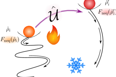
Figure 1: For a general quantum state, one can construct a unitary transformation $\hat{U}$, which increases the state’s non-equilibrium free energy and eliminates the overlap with a set of slow-decaying modes of the generator. This leads to exponentially faster thermalisation and a genuine quantum Mpemba effect.

Recently work has been undertaken to generalise the Mpemba effect to quantum dynamics. The phenomenon and the framework generalise naturally to open quantum systems Nava and Fabrizio (2019); Carollo et al. (2021); Bao and Hou (2022); Manikandan (2021); Kochsiek et al. (2022); Ivander et al. (2023); Chatterjee et al. (2023a, b); Wang and Wang (2024); Caceffo et al. (2024); Strachan et al. (2024) and this has recently been explored experimentally in ion traps Shapira et al. (2024); Zhang et al. (2024). However, it should be stated that very few of these studies focus specifically on thermalisation but rather more generally on anomalous relaxation to general fixed points. Another series of works have investigated a quantum Mpemba-like effect in isolated systems, related to symmetry restoration in quenched dynamics starting from states that break the symmetry of the generating Hamiltonian Ares et al. (2023); Murciano et al. (2024); Yamashika et al. (2024); Liu et al. (2024); Joshi et al. (2024).

In this letter, we focus specifically on Davies maps which are a particular class of continuous-time quantum dynamical semigroups. These maps rigorously describe the thermalisation of a quantum system when weakly coupled to a heat bath Davies (1979); Roga et al. (2010) and are often said to be the quantum equivalent of classical Glauber dynamics. The special mathematical properties of these maps allow us to identify a unique quantum Mpemba effect which stems from the sub-block structure of the generator in the energy eigenbasis. Starting from a state that has coherences, we show how a unitary transformation can transform the state to generate an exponential speed-up which will always occur when the spectral gap of the generator is defined by a complex eigenpair. When the transformed state has a higher non-equilibrium free energy Donald (1987); Esposito and Van den Broeck (2011); Parrondo et al. (2015) the dynamics give rise to a genuine quantum Mpemba effect (see Fig. 1). Furthermore, we study the division of the irreversible entropy production Spohn (1978); Landi and Paternostro (2021) into coherent and incoherent parts Santos et al. (2019); Francica et al. (2019). Our findings are illustrated on single qubit and many-qubit examples.

Consider a quantum Markovian master equation that evolves a density matrix $\hat{\rho}(t)$

$$\frac{d\hat{\rho}(t)}{dt}=\mathcal{G}\hat{\rho}(t).$$ (1)

Here $\mathcal{G}$ is the generator, known as the Lindbladian, consisting of a unitary part and a dissipative part such that $\mathcal{G}=i\delta+\mathcal{D}$ with $\delta(\mathord{\cdot})=-[\hat{H},\mathord{\cdot}]$, $\hat{H}$ being the system Hamiltonian and $\mathcal{D}(\mathord{\cdot})=\sum_{l}\hat{L}^{{\vphantom{\dagger}}}_{l}(\mathord{\cdot})\hat{L}^{\dagger}_{l}-\frac{1}{2}\{\hat{L}^{\dagger}_{l}\hat{L}^{{\vphantom{\dagger}}}_{l},(\mathord{\cdot})\}$, where $\hat{L}_{k}$ are the so-called jump operators. Using the generator we can write down the general evolution of an initial density matrix $\hat{\rho}_{i}$ as

$$\hat{\rho}(t)=e^{\mathcal{G}t}\hat{\rho}_{i}=\hat{\tau}+\sum_{k=2}^{D^{2}}\Tr(\hat{l}_{k}\hat{\rho}_{i})\hat{r}_{k}e^{\lambda_{k}t}\>,$$ (2)

where $D=\mathrm{dim}(\hat{H})$ and we assume that $\hat{\tau}$ is the unique steady state which is the right eigenoperator of the generator $\mathcal{G}$ associated with the zero eigenvalue. Here $\hat{l}_{k}$ and $\hat{r}_{k}$ are the left and right eigenoperators corresponding to the eigenvalue $\lambda_{k}$ such that $\mathcal{G}[\hat{r}_{k}]=\lambda_{k}\hat{r}_{k}$ and $\mathcal{G}^{\dagger}[\hat{l}_{k}]=\lambda_{k}\hat{l}_{k}$ where $\mathcal{G}^{\dagger}$ is the adjoint generator that acts on observables rather than states. The superoperator $\mathcal{G}$ preserves the hermiticity of $\hat{\rho}(t)$, which implies that if $\lambda_{k}$ is a complex eigenvalue then $\lambda^{*}_{k}$ is also. We order the eigenvalues in ascending order according to the modulus of their real part such that $0=\lambda_{1}<|\real(\lambda_{2})|\leq|\real(\lambda_{3})|\leq\dots$. The spectral gap is then $\absolutevalue{\real(\lambda_{2})}$ and defines the longest timescale in the system such that $|\hat{\rho}(t)-\hat{\tau}|\propto\exp(\Re{\lambda_{2}t})$. In Carollo et al. (2021) the authors show that an exponential speed up to the steady state can be achieved by finding a unitary that acts on the initial state such that

$$\Tr(\hat{l}_{2}\hat{U}\hat{\rho}_{i}\hat{U}^{\dagger})=0,$$ (3)

so that $|\hat{\rho}(t)-\hat{\tau}|\propto\exp(\Re{\lambda_{3}t})$. The key assumptions in Carollo et al. (2021) were a pure initial state and a spectral gap defined by a real eigenvalue. When the lowest eigenmodes of the generator form a complex conjugate pair at long times one has

$$\begin{split}\hat{\rho}(t)\propto&\;\hat{\tau}+e^{\real(\lambda_{2})t}\times\\ &\left(\Tr(\hat{l}_{2}\hat{\rho}_{i})\hat{r}_{2}e^{i\imaginary(\lambda_{2})t}+\Tr(\hat{l}^{\dagger}_{2}\hat{\rho}_{i})\hat{r}_{2}^{\dagger}e^{-i\imaginary(\lambda_{2})t}\right),\end{split}$$ (4)

so for a strong Mpemba effect, one would need to find a unitary such that both $\Tr(\hat{l}^{\dagger}_{2}\hat{U}\hat{\rho}_{i}\hat{U}^{\dagger})=0$ and $\Tr(\hat{l}_{2}\hat{U}\hat{\rho}_{i}\hat{U}^{\dagger})=0$ Kochsiek et al. (2022). As argued in Kochsiek et al. (2022), $\hat{\l}_{2}$ is non-Hermitian so the strong Mpemba effect cannot be found using the same logic as in Carollo et al. (2021). Here we demonstrate an alternative route to obtain such a unitary which exploits the mathematical structure of the generator in thermalising open systems.

We consider Davies maps, which are defined by two properties. First, the unitary and dissipative part of the generator commute, and second they obey quantum detailed balance Alicki (1976) with respect to the thermal state $\hat{\tau}_{\beta}=e^{-\beta\hat{H}}/Z$, with $Z=\text{Tr}\left(\text{exp}\left(-\hat{H}\beta\right)\right)$. Mathematically quantum detailed balance means that, given two arbitrary operators $\hat{A}$ and $\hat{B}$, the unitary and dissipative parts of the generator obey $\langle\hat{A},\mathcal{D}^{\dagger}(\hat{B})\rangle_{\hat{\tau}_{\beta}}=\langle\mathcal{D}^{\dagger}(\hat{A}),\hat{B}\rangle_{\hat{\tau}_{\beta}}$ and $[\hat{H},\hat{\tau}_{\beta}]=0$, where $\langle\hat{A},\hat{B}\rangle_{\hat{\tau}_{\beta}}=\Tr(\hat{\tau}_{\beta}\hat{A}^{\dagger}\hat{B})$ is the Kubo-Martin-Schwinger (KMS) inner product. The eigenmatrices of the unitary part $\delta$ are the elemental matrix units $|n\rangle\langle m|$ with eigenvalues $\omega_{nm}=E_{n}-E_{m}$. Since this is a Davies map, the dissipative part $\mathcal{D}$ shares a common eigenspace with $\delta$. Furthermore, if the Hamiltonian is non-degenerate, then the overall Davies map $e^{\mathcal{G}t}$ is block diagonal in the energy eigenbasis. We can write $\mathcal{G}=\mathcal{G}_{P}\mathop{\oplus}\mathcal{G}_{C}$ where $\mathcal{G}_{P}=\mathcal{D}_{P}$ is the population subblock, whose right eigenmatrices are diagonal in the energy eigenbasis $|n\rangle\langle n|$ and $\mathcal{G_{C}}=i\delta+\mathcal{D}_{C}$ is the coherence subblock. Note that due to the detailed balance condition the eigenvalues corresponding to the off-diagonal eigenmatrices of $\mathcal{D}_{C}$ are real whereas imaginary eigenvalues are due to the unitary part $\delta$. The slowest decaying modes shown in Eq. 4 and indeed more generally $\hat{r}_{i}$ for $i\geq 2$ will be off-diagonal matrices in the energy eigenbasis. This ensures that they are traceless which guarantees that the dynamics preserves normalisation at all times. However not only does $\delta$ commute with $\mathcal{D}$, it also commutes with $\mathcal{D}^{\dagger}$. This means that the left eigenvectors of $\mathcal{G_{C}}$ are also purely off-diagonal matrices in the energy eigenbasis since $\mathcal{G}^{\dagger}[\hat{l}_{k}]=\lambda_{k}\hat{l}_{k}$.

We now state our first finding: given an initial state $\hat{\rho}_{i}$ which has coherences in the energy eigenbasis, under an evolution with a Davies generator which has a spectral gap defined by the real part of a complex eigenpair, an exponential speed up towards the fixed point can always be achieved if a unitary $\hat{U}$ is performed to bring the state to be diagonal in the energy eigenbasis. Since all $\hat{l}_{m}$ with $\lambda_{m}\in\mathbb{C}$ are purely off diagonal matrices in the energy eigenbasis then all associtated amplitudes will be simultaneously eliminated $\Tr(\hat{l}_{m}\hat{U}\hat{\rho}_{i}\hat{U}^{\dagger})=0$.

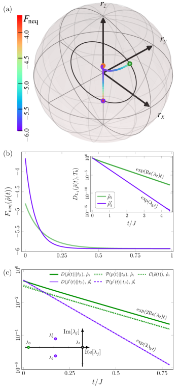
Figure 2: The quantum Mpemba effect in a single-qubit system. a) Bloch sphere representation of the equilibration of a random state $\hat{\rho}_{i}$ (green dot) and the transformed state $\hat{\rho}_{i}^{\prime}=\hat{U}\hat{\rho}_{i}\hat{U}^{\dagger}$ (purple dot) towards the thermal steady state (orange dot). The non-equilibrium free energy $F_{\mathrm{neq}}$ for the two thermalisation processes is represented by the color scheme. b) $F_{\mathrm{neq}}$ is initially higher for the optimized state (purple line), but drops below the random state’s one (green line) at a later time. This crossing shows the occurrence of a genuine quantum Mpemba effect. Inset: The $L_{1}$-distances from the steady state indicate that $\hat{\rho}_{i}$ thermalises exponentially faster than $\hat{\rho}_{i}^{\prime}$. c) Dynamics of the total entropy production $D$ and its classical $\mathcal{P}$ and coherent $\mathcal{C}$ contributions. The rotation $\hat{U}$ yields an exponential speed up. Inset: spectrum of the Davies map $\mathcal{G}$ for a single qubit. Here $h_{0}=1.093$, $h_{\textrm{rand}}=(1.317,-0.208,0.004)$, $\boldsymbol{r}_{i}=(0.738,0.293,0.606)$, $\boldsymbol{r}_{i}^{\prime}=(0.,0.,-0.528)$, and $T_{b}=10J.$

We want to stress an essential point: an exponential speedup in itself does not constitute a genuine Mpemba effect. In the original breakthrough paper Lu and Raz (2017), which focuses on thermodynamics, the effect is defined according to states with three temperatures $T_{b}<T_{c}<T_{h}$ which pertain to the fixed point, colder and hotter initial states, respectively. A Mpemba effect occurs if some time $t_{m}$ exists after which $D[{\hat{\rho}}^{h}(t),T_{b}]<D[\hat{\rho}^{c}(t),T_{b}]$. Here $D[\hat{\rho}(t),T]$ denotes a distance measure between the time-evolving state and the fixed point. Since we are dealing with non-equilibrium quantum states with possible coherences in the energy eigenbasis we do not have any initial notion of temperature. We have one point of equilibrium, namely the fixed point $\hat{\tau}_{\beta}$. For quantum dynamics, we propose to use the non-equilibrium free energy which is defined as

$$F_{\textrm{neq}}(\hat{\rho}(t))=\Tr(\hat{H}\hat{\rho}(t))+\frac{1}{\beta}\Tr(\hat{\rho}(t)\ln\hat{\rho}(t)).$$ (5)

We consider the initial scenario $F_{\textrm{neq}}(\hat{\rho}^{\prime}(t_{0}))>F_{\textrm{neq}}(\hat{\rho}(t_{0}))>F_{\textrm{eq}}$ where $\hat{\rho}^{\prime}(t_{0})=\hat{U}\hat{\rho}(t_{0})\hat{U}^{\dagger}$ is the state following unitary transformation and $F_{\textrm{eq}}=-\beta^{-1}\ln Z$ is the equilibrium free energy of the fixed point. A quantum Mpemba effect occurs if some time $t_{m}$ exists such that $F_{\textrm{neq}}(\hat{\rho}^{\prime}(t))<F_{\textrm{neq}}(\hat{\rho}(t))$ for all times $t>t_{m}$. We call this a genuine quantum Mpemba effect to differentiate it from exponential speedups achieved by other transformations. We emphasize that for the speedup to be a quantum Mpemba effect the non-equilibrium free energy curves need to cross in time. The non-equilibrium free energy has several additional features that make it ideal to define and analyse the quantum Mpemba effect. First of all, it can be written as

$$F_{\textrm{neq}}(\hat{\rho}(t))=\beta^{-1}D(\hat{\rho}(t)||\hat{\tau}_{\beta})+F_{\textrm{eq}}(\hat{\tau}_{\beta}),$$ (6)

where $D(\hat{\rho}||\hat{\sigma})=\Tr[\hat{\rho}(\ln\hat{\rho}-\ln\hat{\sigma})]$ is the quantum relative entropy. The Klein inequality guarantees the positivity of the relative entropy, ensuring that $F_{\textrm{neq}}(\hat{\rho}(t))\geq F_{\textrm{eq}}(\hat{\tau}_{\beta})$ $\forall t$. The quantum relative entropy is a very stringent measure of the distinguishability of two quantum states. While not itself a metric, it still upper bounds the trace distance via Pinsker’s inequality $D(\hat{\rho}||\hat{\sigma})\geq|\lvert\hat{\rho}-\hat{\sigma}\rvert\rvert_{1}^{2}/2$, which captures the optimal distinguishability of quantum states with a single measurement. In addition, Eq. 5 gives us a prescription to find operations that transform an initial state to a state that has both a higher $F_{\text{neq}}$ and also is diagonal in the energy eigenbasis. A simple operation that does this is a unitary which diagonalises the state in the energy eigenbasis and then does a population inversion (see Appendix A). When the generator has a spectral gap defined by a complex eigenpair this will always yield a quantum Mpemba effect since all overlaps with coherent modes go to zero. Finally, not only is the non-equilibrium free energy directly connected to the Spohn entropy production rate Spohn (1978) as $\Pi=-\beta^{-1}dF_{\textrm{neq}}(\hat{\rho}(t))/dt$, as shown in Santos et al. (2019); Francica et al. (2019) and Appendix B the total irreversible entropy produced can be divided as

$$D(\hat{\rho}(t)||\hat{\tau}_{\beta})=\mathcal{P}(p(t)||\hat{\tau}_{\beta})+\mathcal{C}(\hat{\rho}(t)),$$ (7)

where $\mathcal{P}(p(t)||t_{\beta})=\sum_{n}p_{n}(t)\ln\frac{p_{n}(t)}{t^{\beta}_{n}}$ is the classical relative entropy of the time-evolving population vector and the thermal state and $\mathcal{C}(\hat{\rho}(t))=S(\Delta(\hat{\rho}(t)))-S(\hat{\rho}(t))$ is known as the relative entropy of coherence where $\Delta(\hat{\rho}_{s}(t))$ is the state dephased in the systems’ energy eigenbasis. This is known to be an operational measure of quantum coherence Streltsov et al. (2017).

In the following, we consider the thermalization of single and multi-qubit systems. The characteristic energy scale is $J$ and we set $k_{B}=1$.

Example 1: Single Qubit

The qubit is prepared in a random state $\hat{\rho}_{i}=1/2(\mathds{1}+\boldsymbol{r}\cdot\hat{\boldsymbol{\sigma}})$, where $\boldsymbol{r}$ is the Bloch vector and $\hat{\boldsymbol{\sigma}}$ is the vector containing the three Pauli matrices. The thermalisation is described by a unitary part governed by a random Hamiltonian $\hat{H}=J(h_{0}\mathds{1}+\boldsymbol{h}_{\textrm{rand}}\cdot\hat{\boldsymbol{\sigma}})$ and a dissipative part $\mathcal{D}$ defined according to the Davies map for a bath at temperature $T_{b}$ (see Appendix C for details). We perform a unitary $\hat{U}$ on $\hat{\rho}_{i}$ which rotates the Bloch vector to $\boldsymbol{r}_{i}^{\prime}$ and brings it to a new state $\hat{\rho}_{i}^{\prime}$ diagonal in the energy eigenbasis with the eigenvalues in ascending order. The thermalisation dynamics of both states are pictured on the Bloch sphere in Fig. 2(a). The color bar indicates the non-equilibrium free energy $F_{\mathrm{neq}}$, which is shown also in panel (b). The crossing of the two lines indicates a genuine quantum Mpemba effect. The inset shows the $L_{1}$-distance from the steady state $D_{L_{1}}[\hat{\rho}(t),T_{b}]=\sum_{i,j}\absolutevalue{\hat{\rho}^{ij}(t)-\hat{\tau}_{\beta}^{ij}}$, indicating that the thermalisation for the transformed state $\hat{\rho}_{i}^{\prime}$ is exponentially accelerated. We now study the division of the entropy production defined by  Eq. 7 in Fig. 2(c). It can be seen that for the transformed state $\hat{\rho}_{i}^{\prime}$ the coherent contribution is zero (since the overlap with the coherent modes has been eliminated) and the classical entropy production rate is exponentially accelerated from $\real(\lambda_{2})$ to $\lambda_{3}$. The spectrum of the Davies map is shown as an inset. Note that for a single qubit, at any temperature $T_{b}$ the spectral gap is defined by a complex eigenpair.

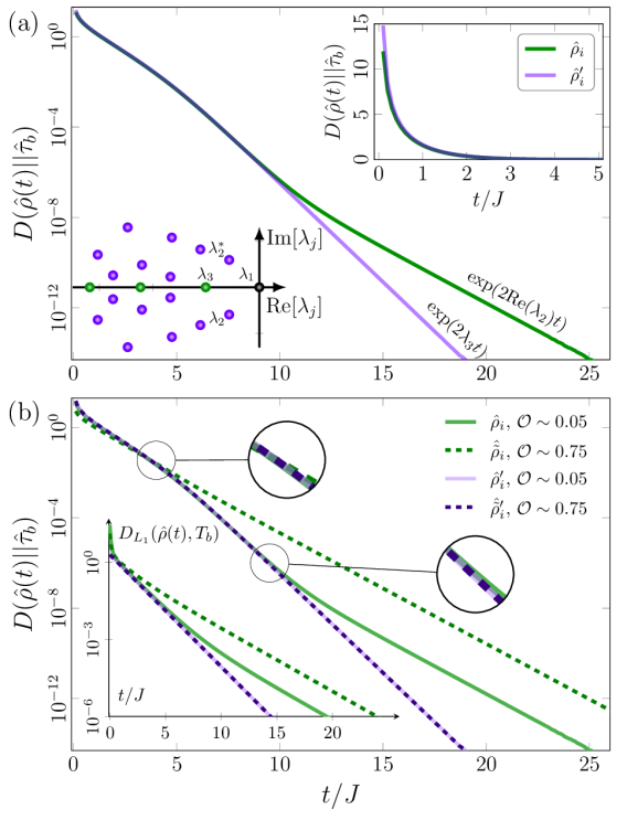
Figure 3: The quantum thermal Mpemba effect in a many-qubit system manifests at different timescales. (a) Same as Fig. 2 (b)-(c) for the transverse field Ising model with anisotropy at the critical point $h=J$ with $L=5$ spins and bath temperature $T_{b}=0.1\,J$. The rotation $\hat{U}$ allows for an exponential speedup governed by $\lambda_{3}$ that shows up at timescales much larger than the single qubit case. Inset: first $20$ eigenvalues of the spectrum of the Davies map $\mathcal{G}$. (b) An initial state with a large overlap with the two slowest decaying modes $\mathcal{O}=\absolutevalue{\Tr(\hat{l}^{\dagger}_{2}\hat{\rho}_{i})}+\absolutevalue{\Tr(\hat{l}_{2}\hat{\rho}_{i})}$ achieves the speedup sooner than one with a small overlap. For $\mathcal{O}\sim 0.05$ (full green line), the curves for the total entropy production cross around $t/J\sim 10$, while with $\mathcal{O}\sim 0.75$ (dashed green line), they coalesce at half of this time.

Example 2: Many Qubits

We now shift our focus to a more complex system and consider a transverse-field Ising model (TFIM) with open boundary conditions $\hat{H}=-J\sum_{j=1}^{L-1}\hat{\sigma}^{z}_{j}\hat{\sigma}^{z}_{j+1}+h\sum_{j=1}^{L}\hat{\sigma}^{x}_{j}$. We construct a random mixed state $\hat{\rho}_{i}$ by averaging over $1000$ random pure states. Then, as for the single qubit case, we obtain the transformed state $\hat{\rho}_{i}^{\prime}$ by applying $\hat{U}$. In panel (a) of Fig. 3 we compute the irreversible entropy production. The main difference to the single qubit case is that since the overlap of the random state $\hat{\rho}_{i}$ with the slowest mode, $\hat{l}_{2}$, is small, the difference with the transformed state manifests only at later a time. The situation changes when one considers an initial state $\hat{\tilde{\rho}}_{i}$ which has a larger overlap with $\hat{l}_{2}$. We construct such a state by applying a metropolis-based transformation, which is explained in Appendix D. The dashed green line in panel (b) shows that, similarly to the single qubit case, the exponential difference in the thermalisation speed of $\hat{\tilde{\rho}}_{i}$ and $\hat{\tilde{\rho}}_{i}^{\prime}$ is evident already at short times.

Conclusion

We have demonstrated that a quantum Mpemba effect can be engineered by exploiting the sub-block structure of the generator in thermalising open Markovian systems. We highlight the non-equilibrium free energy as a central thermodynamic object to both define and study the effect in open quantum systems. When the spectral gap of a Davies generator is defined by a complex eigenpair a unitary operation can always be found on an initial state which simultaneously raises the free energy and provides exponentially quicker thermalisation. The work presented here not only enhances our understanding of the effect in quantum systems and should inspire further studies from the perspective of quantum thermodynamics, but it could also prove useful in dissipative state engineering protocols Verstraete et al. (2009); Harrington et al. (2022); Edo and Wu (2024).

Appendix A Transforming the initial state

In this appendix, we provide more details about the unitary transformation we perform on the initial state and prove that it always increases the non-equilibrium free energy.

In the main text, we argued that to achieve asymptotically, exponentially faster relaxation when the spectral gap is defined by a complex eigenpair, we needed to perform a rotation such that the overlap with the slowest decaying modes go to zero i.e. $\Tr(\hat{l}_{2}\hat{U}\hat{\rho}_{i}\hat{U}^{\dagger})=0$ and $\Tr(\hat{l}^{\dagger}_{2}\hat{U}\hat{\rho}_{i}\hat{U}^{\dagger})=0$. We consider a unitary operator divided into two separate unitary operations

$$\hat{U}=\hat{U}_{2}\hat{U}_{1},$$ (8)

where $\hat{U}_{1}$ achieves the exponential, asymptotic speed up to relaxation and $\hat{U}_{2}$ ensures that the rotated state will have a higher non-equilibrium free energy than the initial state. The unitary $\hat{U}_{1}$ diagonalises the density matrix in the energy eigenbasis;

$$\hat{U}_{1}\hat{\rho}_{i}\hat{U}_{1}^{\dagger}=\hat{\Lambda},$$ (9)

where $\hat{\Lambda}$ is the diagonal matrix of eigenvalues of the density operator. This diagonalisation removes overlaps with all coherent modes, achieving an exponential speed-up if the spectral gap is defined by the real part of a complex eigenpair. We define $\hat{U}_{2}$ to swap the populations of the diagonalised density matrix, generating a population inversion.

To get a genuine Mpemba effect we required our rotated state to have a higher non-equilibrium free energy $F_{\text{neq}}(\hat{\rho})$ than the initial state. We will now show that the rotation defined above will increase the non-equilibrium free energy of an arbitrary initial state $\hat{\rho}_{i}$. We need only compare the relative entropy of the states before and after the rotation, i.e.

$$D(\hat{\rho}_{i}||\hat{\tau}_{\beta})\leq D(\hat{\rho}^{\prime}||\hat{\tau}_{\beta}).$$ (10)

Since $\hat{U}$ is unitary, it does not change the von Neumann entropy of $\hat{\rho}_{i}$. With that, we need to show

$$\text{Tr}[\hat{\rho}_{i}\text{ln}(\hat{\tau}_{\beta})]\geq\text{Tr}[\hat{\rho}^{\prime}\text{ln}(\hat{\tau}_{\beta})].$$ (11)

As the thermal state is diagonal in the energy eigenbasis and the populations are non-increasing, comparing the free energies is equivalent to comparing the populations before and after the rotation. The population distribution of the thermal equilibrium state is in decreasing order. Thus, to maximise $F_{\text{neq}}$, the populations of $\hat{\rho}^{\prime}$ need to be ordered in increasing value, i.e. a complete population inversion.

To demonstrate that the unitary $\hat{U}_{2}$ produces a state with the desired populations, we use the concept of majorisation Bhatia (1997). Denote $p^{\downarrow}$ to be the permutation of the distribution $p$ with values in descending order. One distribution $p$ is said to majorise another distribution $r$, $p\succ r$ if

$$\sum_{j=1}^{k}p^{\downarrow}_{j}\geq\sum_{i=1}^{k}r^{\downarrow}_{j}\>\forall\>k.$$ (12)

The probability distribution $p$ majorises $r$ if it is “less spread out”. As the thermal state populations in Eq. 11 are diagonal matrices with decreasing populations, they act as weights on the population probabilities of the density matrices. If the diagonalised state majorises any unitary transformation, then the full population invertion maximises the non-equilibrium free energy given the constraint of unitary operations. We are interested in any arbitrary unitary from the population-inverted state

$$\sum_{k}\bra{k}\hat{U}\hat{\rho}^{\prime}\hat{U}^{\dagger}\ket{k}=p_{\sigma},$$ (13)

where $\ket{k}$ are the eigenvectors of the Hamiltonian and $p_{\sigma}$ are the populations of a unitarily connected density matrix. We expand $\hat{\rho}^{\prime}$ into its eigenbasis

$$\sum_{r}\bra{k}\hat{U}\ket{r}p_{r}\bra{r}\hat{U}^{\dagger}\ket{k} =\sum_{r}|\bra{k}\hat{U}\ket{r}|^{2}p_{r}$$

$$=\sum_{r}S_{kr}p_{r}=p_{\sigma},$$ (14)

where $\hat{S}$ is a doubly stochastic matrix that maps the probability distribution $p_{r}$ to the probability distribution $p_{\sigma}$. From the Hardy-Littlewood-Polya inequality Hardy et al. (1934) such a doubly stochastic matrix exists if and only if the distribution $p_{r}$ majorises the distribution $p_{\sigma}$. Thus this final state has a higher non-equilibrium free energy than any other state connected by a unitary rotation with equality if and only if the initial state is diagonal in the energy eigenbasis with a full population inversion.

Appendix B Relative entropy and non-equilibrium free energy

In this appendix, we show how the non-equilibrium free energy is written in terms of relative entropy. This is used extensively in quantum and classical stochastic thermodynamics Esposito and Van den Broeck (2011); Parrondo et al. (2015) but to the authors’ knowledge, the connection was first highlighted in the literature by Donald in the 80s Donald (1987). Consider the internal energy $U$ of an arbitrary, possibly time-dependent, state $\hat{\rho}(t)$. We can always write the expression by introducing a thermal state $\hat{\tau}_{\beta}$ as

$$\begin{split}U(\hat{\rho}(t))&=-\beta^{-1}\Tr[\hat{\rho}(t)\log e^{-\beta\hat{H}}]\\ &=-\beta^{-1}\Tr[\hat{\rho}(t)\log\frac{e^{-\beta\hat{H}}}{Z}]-\beta^{-1}\Tr(\hat{\rho}(t)\log{Z})\\ &=-\beta^{-1}\Tr[\hat{\rho}(t)\log\hat{\tau}_{\beta}]-\beta^{-1}S(\hat{\rho}(t))+\beta^{-1}S(\hat{\rho}(t))\\ &+F_{eq}\\ &=\beta^{-1}D(\hat{\rho}(t)||\hat{\tau}_{\beta})+\beta^{-1}S(\hat{\rho}(t))+F_{eq},\end{split}$$ (15)

where on the third line we have added and subtracted a von Neumann entropy term $S(\hat{\rho})=-\Tr(\hat{\rho}\log{\hat{\rho}})$ and we have introduced the relative entropy between the state and the thermal state. The non-equilibrium free energy is then computed from $F_{\text{neq}}(\hat{\rho}(t))=U(\hat{\rho}(t))-\beta^{-1}S(\hat{\rho}(t))$ and we can use the expression for the internal energy above so that

$$F_{\textrm{neq}}(\hat{\rho}(t))=\beta^{-1}D(\hat{\rho}(t)||\hat{\tau}_{\beta})+F_{\text{eq}}$$ (16)

as used in the main text. When $\hat{\rho}(t)=\hat{\tau}_{\beta}$ the equilibrium free energy is recovered $F_{\text{eq}}=\beta^{-1}\Tr(\log{Z})$. For more on the physical interpretation of $F_{\text{neq}}$ see Parrondo et al. (2015).

Appendix C Explicit form of the Davies map

For pedagogical purposes, in this section we give some more details regarding Davies maps studied in the main text. For Markovian open quantum systems, the dynamics of the system’s density matrix $\hat{\rho}$ is governed by the Lindblad equation

$$\frac{d\hat{\rho}(t)}{dt}=\mathcal{G}\hat{\rho}(t)=-i[\hat{H},\hat{\rho}(t)]+\sum_{l}\hat{L}^{{\vphantom{\dagger}}}_{l}\hat{\rho}(t)\hat{L}^{\dagger}_{l}-\frac{1}{2}\{\hat{L}^{\dagger}_{l}\hat{L}^{{\vphantom{\dagger}}}_{l},\hat{\rho}(t)\},$$ (17)

where $\mathcal{G}$ is the generator, $\hat{H}$ is the system’s Hamiltonian, and $\hat{L}^{{\vphantom{\dagger}}}_{l}$ are the jump operators describing the influence of the environment on the system Manzano (2020). An important class of Lindbladians, known as Davies maps Davies (1979), describes the thermalisation of a quantum system when weakly coupled to a heat bath. The fixed point of Davies maps is the thermal state at inverse temperature $\beta$

$$\hat{\tau}_{\beta}=\exp\left(-\beta\hat{H}\right)/Z,$$ (18)

where $Z$ is the partition function. In the following, it is convenient to work in the Hamiltonian eigenbasis $\{\ket{n}\}$. We want to show that Davies maps are characterised by the following jump operators:

$$\hat{L}^{(1)}_{nm}(\beta)=\underbrace{\left(1\mp f^{\pm}(\beta,h_{m}-h_{n})\right)^{1/2}}_{\alpha_{nm}^{(1)}}\ket{n}\bra{m}$$ (19)

$$\hat{L}^{(2)}_{nm}(\beta)=\underbrace{\left(f^{\pm}(\beta,h_{m}-h_{n})\right)^{1/2}}_{\alpha_{nm}^{(2)}}\ket{m}\bra{n},\hskip 14.22636pt\text{with }m<n,$$

where $h_{n}$ are the eigenvalues of the Hamiltonian and $f^{\pm}(\beta,h_{n})=1/(\exp(\beta h_{n})\pm 1)$ are the Fermi and the Bose distribution functions. To do so, we have to prove that $\mathcal{G}\left[\hat{\tau}_{\beta}\right]=0$. Since $\hat{\tau}_{\beta}$ commutes with $\hat{H}$, we need to consider only the dissipator $\mathcal{D}(\mathord{\cdot})=\sum_{l}\hat{L}^{{\vphantom{\dagger}}}_{l}(\mathord{\cdot})\hat{L}^{\dagger}_{l}-\frac{1}{2}\{\hat{L}^{\dagger}_{l}\hat{L}^{{\vphantom{\dagger}}}_{l},(\mathord{\cdot})\}$ and have to show that $\mathcal{D}(\hat{\tau}_{\beta})=\sum_{m<n}\mathcal{D}^{(1)}_{nm}(\hat{\tau}_{\beta})+\mathcal{D}^{(2)}_{nm}(\hat{\tau}_{\beta})=0$. Indeed, for every $(n,m)$ the dissipator contributions from the jump operators $\hat{L}^{(1)}_{nm}$ and $\hat{L}^{(2)}_{nm}$ cancel out:

$$\mathcal{D}^{(1)}_{nm}(\hat{\tau}_{\beta})+\mathcal{D}^{(2)}_{nm}(\hat{\tau}_{\beta})=$$

$$\frac{1\mp f^{\pm}(h_{m}-h_{n})}{\mathcal{N}}e^{-\beta h_{m}}\left(\ket{n}\bra{n}-\ket{m}\bra{m}\right)$$

$$+\frac{f^{\pm}(h_{m}-h_{n})}{\mathcal{N}}e^{-\beta h_{n}}\left(\ket{m}\bra{m}-\ket{n}\bra{n}\right)=0,$$

where we have used that $(1\mp f^{\pm}(h_{m}-h_{n}))e^{-\beta(h_{m}-h_{n})}=f^{\pm}(h_{m}-h_{n})$, which is the thermal detailed balance condition. Thus, the Lindbladian specified by the jump operators Eq. 19 has the thermal state as its fixed point.

Like any Lindbladian, the Davies map can be represented by a non-Hermitian matrix via vectorisation procedure Am-Shallem et al. (2015); Landi et al. (2022) as

$$\hat{\mathcal{G}}=-i\hat{H}\otimes\hat{\mathds{1}}+i\hat{\mathds{1}}\otimes\hat{H}^{\scriptscriptstyle T}+$$ (20)

$$\sum_{l}\hat{L}^{{\vphantom{\dagger}}}_{l}\otimes\left(\hat{L}^{\dagger}_{l}\right)^{\scriptscriptstyle T}-\frac{1}{2}\hat{L}^{\dagger}_{l}\hat{L}^{{\vphantom{\dagger}}}_{l}\otimes\hat{\mathds{1}}-\frac{1}{2}\hat{\mathds{1}}\otimes\left(\hat{L}^{\dagger}_{l}\hat{L}^{{\vphantom{\dagger}}}_{l}\right)^{\scriptscriptstyle T}.$$

As we discuss in the main text, if the Hamiltonian is non-degenerate $\hat{\mathcal{G}}$ can be recast into a block-diagonal form $\hat{\mathcal{G}}=\hat{\mathcal{G}}_{p}\oplus\hat{\mathcal{G}}_{c}$, with $\hat{\mathcal{G}}_{p}$ describing the system’s populations and $\hat{\mathcal{G}}_{c}$ the system’s coherences

$$\hat{\mathcal{G}}=\left(\vbox{\hbox{ \leavevmode\hbox to135.69pt{\vbox to135pt{\text{[drawing]}}}}}\right), 2^{L} 2^{L} 4^{L}-2^{L} 4^{L}-2^{L} 2^{L} 2^{L} 4^{L}-2^{L} 4^{L}-2^{L}$$ (21)

where $L$ is the number of fermions, hard-core bosons, or spin-$1/2$ particles in the system. Moreover, the left eigenmatrices $\hat{l}_{k}$ associated with the system’s populations are diagonal and correspond to real eigenvalues $\lambda_{k}$, while those associated with the system’s coherences are strictly off-diagonal and the relative eigenvalues come in complex conjugate pairs.

Instead of plugging the jump operators Eq. 19 into the general expression for the vectorised Lindbladian Eq. 20, one can also construct the two blocks of the Davies map individually, saving significant computational resources. For this purpose, we define the matrix $\hat{J}$ collecting all the jump operators. For concreteness, for two qubits it reads:

$$\hat{J}=\begin{pmatrix}0&\alpha_{01}^{(2)}&\alpha_{02}^{(2)}&\alpha_{03}^{(2)}\\ \alpha_{10}^{(1)}&0&\alpha_{12}^{(2)}&\alpha_{13}^{(2)}\\ \alpha_{20}^{(1)}&\alpha_{21}^{(1)}&0&\alpha_{23}^{(2)}\\ \alpha_{30}^{(1)}&\alpha_{31}^{(1)}&\alpha_{32}^{(1)}&0\end{pmatrix}.$$ (22)

The coefficients $\alpha^{(1)}_{nm}$ and $\alpha^{(2)}_{nm}$ are obtained from Eq. 19. It can be shown that the populations block $\hat{\mathcal{G}}_{p}$ reads

$$\hat{\mathcal{G}}_{p}=\hat{J}_{2}+\hat{J}_{s},$$ (23)

where $\hat{J}_{2}$ is obtained by squaring $\hat{J}$ elementwise and $\hat{J}_{s}$ is a diagonal matrix with $\hat{J}_{s}[k,k]=-\sum_{i=0}^{2^{L}-1}\left(\hat{J}[i,k]\right)^{2}$.

Let us now construct the coherences block $\hat{\mathcal{G}}_{c}$, which is diagonal in the energy eigenbasis. For this one has to pick all possible $(4^{L}-2^{L})/2$ couples of columns $\hat{J}[:,n]$ and $\hat{J}[:,m]$ with $n=0,1,\dots 2^{L}$ and $m>n$. Each couple of columns $(n,m)$ identifies two elements $\hat{\mathcal{G}}_{p}[k,k]$ and $\hat{\mathcal{G}}_{p}[l,l]$ which are the complex conjugate of one another. The indices of these two elements are $k=m\cdot 2^{L}-m+n-1$ and $l=n\cdot 2^{L}+m-n$. Their real part reads

$$\real(\hat{\mathcal{G}}_{p}[k,k])=\real(\hat{\mathcal{G}}_{p}[l,l])=$$ (24)

$$-\sum_{i=0}^{2^{L}-1}\left(\frac{(\hat{J}[i,n])^{2}}{2}+\frac{(\hat{J}[i,m])^{2}}{2}\right),$$

and their imaginary part is

$$\imaginary(\hat{\mathcal{G}}_{c}[k,k])=\imaginary^{*}(\hat{\mathcal{G}}_{c}[l,l])=i(h_{n}-h_{m}).$$ (25)

Appendix D Metropolis algorithm for Mpemba

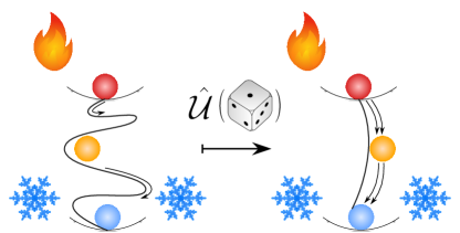
Figure 4: A unitary transformation obtained from a stochastic Metropolis algorithm can exponentially accelerate a relaxation process.

In this article, we have focused on Davies maps and shown how exponential speedups related to a genuine quantum Mpemba effect can be obtained for thermalisation processes. As demonstrated by the vast recent literature Nava and Fabrizio (2019); Carollo et al. (2021); Bao and Hou (2022); Manikandan (2021); Kochsiek et al. (2022); Ivander et al. (2023); Chatterjee et al. (2023a, b); Wang and Wang (2024); Caceffo et al. (2024); Strachan et al. (2024); Shapira et al. (2024); Zhang et al. (2024), however, transformations of initial states that lead to anomalous relaxations in general Lindbladians are of great relevance. Here we introduce a numerical method that generalises Carollo et al. (2021); Kochsiek et al. (2022) to find (possibly multiple) exponential speedups for mixed states evolving with arbitrary Lindbladians.

Given an initial state $\hat{\rho}$ and $K$ left eigenmodes, the goal is to find the unitary transformation $\hat{U}:\>\>\hat{\rho}\to\hat{\rho}^{\prime}$, such that the cost function

$$C=\sum_{k=2}^{K+1}\absolutevalue{\Tr(\hat{l}_{k}\hat{\rho}^{\prime})}$$ (26)

is minimised. A general global unitary transformation acting on $L$ qubits is characterised by $4^{L}$ real parameters. Thus, in order to be able to consider large systems, we assume that the global unitary can be decomposed in terms of single-qubit unitaries:

$$\hat{U}=\prod_{j=1}^{L}\hat{U}_{j}\hskip 14.22636pt\text{with}$$ (27)

$$\hat{U}_{j}(\alpha_{j},\beta_{j},\gamma_{j},\delta_{j})=\exp(i\alpha_{j})\hat{R}_{z}(\beta_{j})\hat{R}_{x}(\gamma_{j})\hat{R}_{z}(\delta_{j}),$$

where $\alpha,\beta,\gamma,\delta\in[0,2\pi]$. With this ansatz, an optimal $\hat{U}$ can be obtained by performing a Metropolis search Metropolis et al. (1953); Press et al. (1992) consisting of the following steps:

1. Initialise a random $\hat{U}$ and an effective temperature $T_{\text{eff}}=1$, rotate $\hat{\rho}$ with $\hat{U}$ and compute the cost function $C$.

2. Pick randomly which qubit $j$ to optimise.

3. For the selected qubit, choose stochastically which parameter $x_{j}\in\{\alpha_{j},\beta_{j},\gamma_{j},\delta_{j}\}$ of $\hat{U}_{j}$ to optimise.

4. Vary the selected parameter $x_{j}\to x_{j}^{\prime}=x_{j}+\delta x_{j}$ by a random increment $\delta x_{j}\in[0,2\pi]$, update $\hat{U}$ and $\hat{\rho}^{\prime}\equiv\hat{U}\hat{\rho}\hat{U}^{\dagger}$ and reevaluate the cost function Eq. 26 with $\hat{\rho}^{\prime}$ .

5. If $C^{\prime}<C$, accept the new unitary $\hat{U^{\prime}}\to\hat{U}$ and update $C^{\prime}\to C$. Otherwise accept the new unitary with probability $p=\exp\left(-\frac{C^{\prime}-C}{T_{\text{eff}}}\right)$.

6. If the new unitary is accepted, decrease the effective temperature by a cooling constant $\tau$: $T_{\text{eff}}\to\tau T_{\text{eff}}$.

7. Repeat steps 4-6 $n$ times (nano iterations: optimising over one parameter).

8. Repeat steps 3-6 $m$ times (micro iterations: optimising over all parameters of a single qubit $j$).

9. Repeat steps 2-6 $LM$ times (macro iterations: optimising over all qubits).

The algorithm is terminated once the cost function has decreased below a threshold $\epsilon$. We dubbed this algorithm unitary Metropolis. The generalisation to fermionic systems is straightforward and consists of taking into account the fermionic anticommutation relations. This can be achieved, for instance, by replacing the single-qubit unitary $\mathds{1}\otimes\mathds{1}_{2}\dots\otimes\hat{U}_{j}\otimes\mathds{1}_{j+1}\dots\mathds{1}_{L}$ in Eq. 27 with $\mathds{1}_{1}\otimes\mathds{1}_{2}\dots\otimes\hat{U}_{j}\otimes\sigma^{z}_{j+1}\dots\sigma^{z}_{L}$, which yields:

$$\hat{U}^{f}=\prod_{j=1}^{L}U_{j}\>\left(\sigma_{j}^{z}\right)^{\text{mod(L-j,2)}}.$$ (28)

Note also that the same method can be applied to bosonic systems with local dimension $d$ by decomposing single-site $d$-dimensional unitary operators $\hat{U}(d)$ into two-level rotations as outlined in Algorithm 1 in Ringbauer et al. (2022).

The algorithm outlined above can be simplified when considering the special class of Lindbladians called Davies maps, which describe thermalisation processes. As we discussed in Appendix C, Davies maps have a block diagonal structure indicating that populations and the coherences of an initial state evolve independently from one another. Thus, when the initial state is diagonal (incoherent) in the energy eigenbasis, the unitary optimization can be substituted by a simpler swap of the state’s populations in the following way:

1. Recast the diagonal part of the incoherent $(2^{L}\times 2^{L})$ initial state $\hat{\rho}$ into a $2^{L}$-dimensional vector and do the same for the targeted diagonal left eigenmatrices $\hat{l}_{k}$. We will indicate the vectorised matrices with double brackets $\hat{\cdot}\to||\cdot\rangle\rangle$.

2. Evaluate the cost function $C\equiv\sum_{k=1}^{K=1}\absolutevalue{\langle\langle l_{k}|\rho\rangle\rangle}$ and initialise an effective temperature $T_{\text{eff}}=1$.

3. Randomly select four integers $n_{1},n_{2},n_{3},n_{4}\in[0,d]$ representing the indices of four entries of $||\rho\rangle\rangle$ and perform a random permutation $P\left(n_{1},n_{2},n_{3},n_{4}\right)=\left(\tilde{n}_{1},\tilde{n}_{2},\tilde{n}_{3},\tilde{n}_{4}\right)$, excluding the trivial permutation $\left(\tilde{n}_{1},\tilde{n}_{2},\tilde{n}_{3},\tilde{n}_{4}\right)=\left(n_{1},n_{2},n_{3},n_{4}\right)$.

4. Compute $||\rho^{\prime}\rangle\rangle$ by swapping the four randomly selected elements of $||\rho\rangle\rangle$ according to the random permutation $P$ and compute the cost function $C^{\prime}$ with the updated state.

5. If $C^{\prime}<C$, accept the new state $||\rho^{\prime}\rangle\rangle\to||\rho\rangle\rangle$ and update $C^{\prime}\to C$. Otherwise accept the new state with probability $p=\exp\left(-\frac{C^{\prime}-C}{T_{\text{eff}}}\right)$.

6. If the new state is accepted, decrease the effective temperature by a cooling constant $\tau$: $T_{\text{eff}}\to\tau T_{\text{eff}}$.

7. Repeat steps $3-6$ until the cost function is reduced below a threshold $\epsilon$.

We refer to this method as swap Metropolis. The same method can be applied to a classical Markovian thermalisation process, the only difference being that the eigenmodes and initial states are already vectors, so step 1. can be skipped. We note that a swap minimisation method (which was not utilised in this work) was imple- mented in Mathematica Schmied (2019).

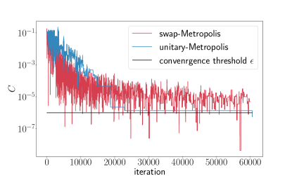
Figure 5: The swap Metropolis and the unitary Metropolis methods applied to the thermalisation of a TFIM with $L=5$ and $h=J$. The swap Metropolis (red line) is used to decrease the overlap of a thermal state with one diagonal eigenmode with a cooling constant $\tau=0.998$. The unitary Metropolis is applied to reduce the overlap of a random state with two off-diagonal eigenmodes with $\tau=0.999$. We set the maximally allowed number of nano iterations to $n=200$, micro iterations to $m=20$, and macro iterations to $M=20$.

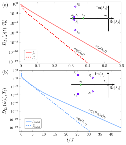
Figure 6: Exponentially accelerated thermalisations after the Metropolis optimisation ( see Fig. 5). Panel (a): the $L_{1}$-distance from the thermal steady state before (full line) and after (dashed line) applying the swap metropolis optimisation during the heating process of a thermal state. Panel (b): the $L_{1}$-distance from the thermal steady state before (full line) and after (dashed line) applying the unitary metropolis optimisation during the thermalisation process of a random mixed state. In both cases, the Metropolis algorithms yield exponential speedups.

We now apply the two Metropolis algorithms to study the thermalisation of a transverse-field Ising model (TFIM)with open boundary conditions $\hat{H}=-J\sum_{j=1}^{L-1}\hat{\sigma}^{z}_{j}\hat{\sigma}^{z}_{j+1}+h\sum_{j=1}^{L}\hat{\sigma}^{x}_{j}$ and set $h=J$ and $L=5$. First, we consider the heating of a thermal state from $T_{i}=1\,J$ to $T_{b}=4\,J$ and use the swap Metropolis algorithm to minimise the overlap of the initial state with a single eigenmode $\hat{l}_{2}$. Then, we study the thermalisation of a random mixed state (obtained by averaging over 1000 random pure states) with $T_{b}=0.1\,J$ and apply the unitary Metropolis to target two modes, $\hat{l}_{2}$ and $\hat{l}_{3}$. Fig. 5 shows that the swap Metropolis already decreases $C$ below $\epsilon=10^{-6}$ after around $5300$ iterations, while the unitary Metropolis crosses the convergence threshold after about $60500$ iterations. We stress that despite the relatively large number of iterations used, both methods have low computational costs. The bottleneck for the investigation of the Mpemba effect is constituted by the diagonalisation of the quantum or classical Liouvillian and not by the minimisation algorithms. In Fig. 6 we show the dynamics of the $L_{1}$-distance from the steady state before and after the swap Metropolis and the unitary Metropolis optimisations. In both cases, it can be seen that exponential speedups are found. In particular, panel (a) shows that since the swap Metropolis algorithm preserves the diagonal structure of the thermal initial state, the transformed state remains orthogonal to the off-diagonal modes and the thermalisation rate is boosted from $\lambda_{2}$ to $\lambda_{5}$.