TwinLiteNet⁺
A Stronger Model for Real-time Drivable Area and Lane Segmentation

Abstract

Semantic segmentation is crucial for autonomous driving, particularly for Drivable Area and Lane Segmentation, ensuring safety and navigation. To address the high computational costs of current state-of-the-art (SOTA) models, this paper introduces TwinLiteNetPlus (TwinLiteNet⁺), a model adept at balancing efficiency and accuracy. TwinLiteNet⁺ incorporates standard and depth-wise separable dilated convolutions, reducing complexity while maintaining high accuracy. It is available in four configurations, from the robust 1.94 million-parameter TwinLiteNet${}^{+}_{\text{Large}}$ to the ultra-compact 34K-parameter TwinLiteNet${}^{+}_{\text{Nano}}$. Notably, TwinLiteNet${}^{+}_{\text{Large}}$ attains a 92.9% mIoU for Drivable Area Segmentation and a 34.2% IoU for Lane Segmentation. These results notably outperform those of current SOTA models while requiring a computational cost that is approximately 11 times lower in terms of Floating Point Operations (FLOPs) compared to the existing SOTA model. Extensively tested on various embedded devices, TwinLiteNet⁺ demonstrates promising latency and power efficiency, underscoring its suitability for real-world autonomous vehicle applications. The code is available on GitHub.

top=1.1in, bottom=1.5in, left=0.7in, right=0.7in

1 Introduction

The advent of methodologies based on deep learning has heralded autonomous vehicles as a burgeoning area within the realms of artificial intelligence and computer vision. In the context of autonomous navigation, the efficacy of the vehicle’s decision-making mechanisms is critically dependent upon the precision with which the system can identify and comprehend its surroundings. Approaches that leverage sensors such as Radar, LIDAR, or cameras have become prevalent for enabling vehicles to perceive their environment during movement. While these technologies are capable of functioning across diverse weather conditions and extracting depth information from the environment, Radar and LIDAR are associated with higher costs in comparison to cameras and, notably, lack the ability to discern colors. This deficiency leads to an increase in the overall cost of the sensor systems for autonomous vehicles without offering the detailed environmental imagery provided by cameras. Consequently, within the domain of practical applications for autonomous vehicles,

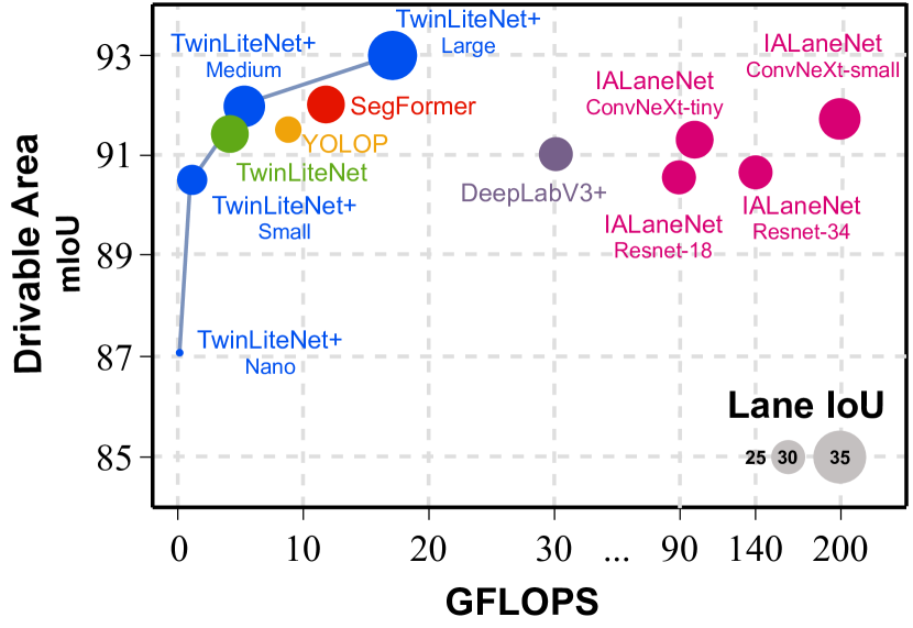
Figure 1: Comparison of evaluation metrics mIoU (Drivable Area Segmentation) - IoU (Lane Segmentation) - GFLOPs of various models on the BDD100K dataset. The x-axis represents the number of GFLOPs of the model, the y-axis represents the mIoU data for the Drivable Area Segmentation task, and the radius of the circle indicates the accuracy for the Lane Segmentation task (the larger the radius, the higher the accuracy).

cameras have remained a principal focus and have undergone more rigorous development, particularly in scenarios where deep learning is extensively employed for image analysis and, more broadly, for advancements in computer vision.

In recent years, techniques related to transformers and convolution-based methods have undergone extensive research in the field of computer vision, particularly for specific tasks such as classification, object detection, and segmentation. While transformers have made significant strides in natural language processing and image analysis tasks, they often introduce high latency and necessitate a substantial number of parameters and extensive data for achieving optimal results. When developing models for autonomous vehicles, where tasks demand both high accuracy and low latency, the low-latency aspect assumes a critical role. Therefore, in the context of autonomous driving, research continues to place a strong emphasis on convolution-based models.

In Advanced Driver Assistance Systems (ADAS), semantic segmentation plays a pivotal role by delineating drivable areas and lane markings. This capability significantly enhances an autonomous vehicle’s navigation and obstacle avoidance, thereby ensuring safer operation. The accurate detection of lane markings and the differentiation between directly drivable lanes and alternate lanes are crucial for facilitating precise steering and lane-change decisions. Although research has produced dedicated models for segmentation tasks within the autonomous driving context, such as drivable area segmentation [1, 2] or lane segmentation [3, 4, 5], achieving promising results, a naive implementation approach would lead to a linear increase in the number of models commensurate with the required task volume. To optimize both accuracy and inference time, recent advancements have favored the adoption of multi-task models over single-task models.

Multi-task models, capable of simultaneously executing drivable area segmentation and lane segmentation [6, 7, 8], alongside incorporating object detection functionalities [9, 10, 11], are garnering significant interest due to their efficiency in handling multiple tasks concurrently. However, recent developments in these models predominantly concentrate on enhancing model accuracy, often overlooking the practical applicability of such models in autonomous vehicle applications. Multi-task models [7][9] are constructed with considerable complexity to facilitate the simultaneous execution of numerous tasks. These models are typically evaluated on high-end hardware, such as RTX3090 and Tesla V100, achieving processing speeds of several tens of frames per second. Nevertheless, these evaluations frequently neglect to address critical considerations for deployment on embedded devices, such as inference speed and power consumption. This oversight presents a substantial impediment to the deployment of embedded systems within autonomous vehicles, where computational resources are inherently constrained. Large-scale models or those not initially conceived for deployment on embedded devices often resort to model compression techniques such as Pruning, 8-bit Quantization, and Knowledge Distillation for implementation on embedded systems. These methods, however, can lead to a degradation of accuracy relative to the original model, and not every model successfully maintains high accuracy post-application of these techniques. To tackle this challenge, this paper introduces a multi-task model tailored for segmentation tasks within the autonomous driving context, designed with an emphasis on efficient execution on devices characterized by limited computational capacity, specifically embedded devices.

In this work, we introduce TwinLiteNet⁺, a model tailored for real-time operation with minimal power consumption and hardware resources, proficient in simultaneously segmenting lanes and drivable areas. This model demonstrates competitive precision in tasks akin to those of similar models. The principal contributions of our research are threefold: (1) We present a lightweight Convolutional Neural Network (CNN) model, optimized for low computational cost, consisting of a singular encoder block and dual decoder blocks for the respective tasks of drivable area and lane segmentation. (2) The model is offered in four distinct configurations, each balancing accuracy with computational efficiency. (3) To validate our model’s applicability in real-world conditions, we deploy and assess its performance in terms of speed and energy efficiency on a range of embedded devices, including the Jetson Xavier and Jetson TX2.

The remainder of the paper is represented as follows: We evaluate relevant models in Section 2 to grasp the benefits and drawbacks in the tasks of Drivable Area Segmentation, and Lane Segmentation with Multi-task approaches. The proposed TwinLiteNet⁺ presents an architecture with methods to boost model performance in Section 3. In Section 4, we conduct experiments on BDD100K dataset and the results show that our TwinLiteNet⁺ models outperform on latency and power efficiency. In the final Section, we provide some conclusions and future development directions.

2 Related works

In this section, we present a brief evaluation of related work, focusing particularly on segmentation models in the context of autonomous vehicles and methods for optimizing deep learning models on embedded devices.

2.1 Semantic Segmentation

Semantic segmentation is a prominent research area extensively explored in the field of computer vision. The main distinction separating it from detection tasks lies in its ability to perform pixel-level classification, involving the labeling of each pixel to delineate objects and their boundaries. Initially, Convolutional Neural Network (CNN) lays the groundwork for effective methods in handling these tasks, with various high-performance models developed for numerous applications [12, 13, 14]. Furthermore, the integration of attention modules [15][16] has opened up powerful approaches for semantic segmentation, significantly enhancing the learning capabilities of segmentation models during training.

2.1.1 Drivable Area Segmentation

Recent works have suggested many efficient approaches for semantic segmentation in self-driving tasks, particularly in drivable area segmentation, surpassing traditional lane segmentation models that can only recognize the road ahead of a vehicle. Both [17, 18] employ deep learning methods to predict drivable area utilizing a ResNet backbone. While the first study enhances semantic information using Feature Pyramid Network (FPN) and Atrous Spatial Pyramid Pooling (ASPP) modules, the second integrates LinkNet [19] and a CycleGAN-based augmentation to improve night-time segmentation. Zhao et al.[1] devise the PSPNet model utilizing the Pyramid Pooling Module (PPM) that applies global average pooling with multiple different bin scales to extract various levels of features for dividing drivable area. To further enhance applicability, ESPNet[13] uses Dilated Convolutions to build an efficient spatial pyramid (ESP) module that can deliver real-time processing and still maintain high accuracy compared to the aforementioned models.

2.1.2 Lane Segmentation

Within the field of autonomous vehicles, lane detection is also among the basic topics for driving perception. Old-fashioned lane-detecting methods have been conducted such as using a color-based method to extract lane boundary [20], or converting to HSI Color [21] to detect lane markings based on thresholds. These conventional methods heavily depend on handcrafted rules and thresholds and often struggle with environmental conditions such as lighting or weather. They require domain insights for parameter tuning and are often unable to adapt to diverse real-road conditions. To solve this, Global Association Network (GANet) [22] is proposed to handle this task from a keypoint-based perspective or [23] introduces a transformer-only method in its framework to enhance lane segmentation through local prior knowledge. In recent years, segmentation-based methods in deep learning have proven to be the most practical approach for many studies. In 2017, Angshuman Parashar et al.[3] proposed Spatial CNN (SCNN) with a new neural network architecture by generalizing traditional deep layer-by-layer to slice-by-slice convolution in feature mapping, allowing information to propagate across pixels along rows and columns within a layer despite time-consuming. On the other hand, Enet-SAD [4] utilizes a self-attention-guided filter method to assist low-level feature maps in learning from high-level feature maps, or recently, road marking methods [24, 25] have also brought much attention from the community. Later on, a novel detector CLRerNet [26] along with a proposed LaneIoU metric are presented to further improve the confidence score.

Although previous research highlighted the initial success of models in the single-task domain, the advantage of leveraging a model to address multiple tasks has led to recent studies demonstrating that a multi-task strategy is more appropriate for real-world applications, particularly when deployed on devices with limited computing capabilities, such as embedded systems. This method allows models to strike a balance between efficiency and complexity while concurrently performing two tasks: segmentation of the driver’s zone and lane detection. Consequently, we introduce an architecture designed with shared encoder blocks that distribute information to various decoder blocks.

2.2 Multi-task Approaches

Considering the shift from single-task models to multi-task frameworks, this approach has become an established strategy for concurrently addressing multiple tasks. It enhances shared representations and leverages the similarities among diverse tasks. The introduction of the BDD100K dataset has propelled research into multi-task models for autonomous driving challenges, leading to the exploration of various models, including those for drivable area segmentation, lane segmentation [8, 6, 7]; drivable area segmentation and scene classification [27, 28]; as well as drivable area segmentation, lane segmentation, and object detection [10, 29, 11]. [10, 29, 11] introduced a model that integrates a YOLO-based shared backbone with an encoder-decoder structure, effectively combining three separate sensory tasks: vehicle detection, drivable area segmentation, and lane detection. A comparable encoder-decoder architecture is also present in Hybridnets [9], which boasts a more lightweight backbone through the use of depth-wise separable convolutions. Recently, CenterPNets [30] has gained attention for its ability to achieve high accuracy and precision with an end-to-end shared multi-task network. However, the previously proposed multi-task models were primarily focused on improving accuracy and were not extensively tested on devices with limited computational capabilities. As a result, directly implementing these models in autonomous vehicle systems continues to pose significant challenges. Contrary to the goals of previous approaches, TwinLiteNet [8] was specifically designed to facilitate real-time implementation on devices with low configurations, particularly embedded systems. With merely 0.44M parameters, this model boasts competitive accuracy in tasks such as lane segmentation and identifying drivable areas. Significantly, it incorporates an ESP encoder, which is based on dilated convolutions, enabling efficient feature extraction with a reduced number of parameters. Despite TwinLiteNet’s streamlined architecture and high efficiency, the simplistic design of its decoder block limits the model’s ability to effectively leverage information during the decoding process. Inspired by TwinLiteNet, our TwinLiteNet⁺ model improves upon the encoder by integrating additional convolutional layers after the Transpose Convolution layer, thereby enhancing feature extraction while still maintaining low computational costs. Moreover, the introduction of skip connection techniques during the decoding phase enables the combination of input and decoding features. Additionally, in Encoder block of TwinLiteNet⁺, Depthwise and dilated convolutions are combined to robustly optimize the model’s latency.

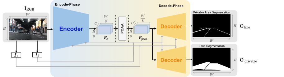
Figure 2: The TwinLiteNet⁺ architecture, as illustrated, comprises two phases. During the Encoding phase, the input image passes through an Encoder block followed by a Partial Class Activation Attention mechanism. In the decode phase, the output from the Encoder is channeled through two identical yet independent Decoder blocks, transforming the feature maps into two separate segmentation maps.

2.3 Optimizing Deep Learning Deployment on Embedded Devices

In recent years, deploying deep learning models on embedded devices has attracted considerable attention within the artificial intelligence community. The computation on these devices is distinguished by its ability to execute processes directly on units that are both cost-effective and task-specific. Despite this advantage, such capabilities are constrained by significant limitations in terms of computational power and storage capacity, presenting substantial challenges for the deployment of deep learning models on these platforms. Prominent model compression techniques, such as 8-bit quantization, pruning, and knowledge distillation, have been devised to enable lower-cost computation without sacrificing accuracy. Quantization, in particular, is a straightforward yet efficacious method that involves performing calculations with fewer bits than the standard 32-bit representation. Post-training quantization enables models, initially trained with 32 bits, to conduct inference at reduced bit levels without necessitating retraining. In contrast, Quantization-aware training incorporates Fake Quantize layers, usually resulting in greater accuracy compared to post-training quantization. However, the latter is preferred for its simplicity, as it obviates the need for retraining the model. Howard et al. introduce MobileNet[31], a class of efficient models tailored for embedded and mobile vision applications, employing depthwise separable convolutions to mitigate computational demands. Recent studies have demonstrated the superiority of Depth-wise dilated separable convolutions over standard Dilation in classification tasks, achieving an accuracy of 67.9% with 123M FLOPs, as opposed to 69.2% accuracy at the cost of 478M FLOPs (an increase of $\times$3.9) with standard Dilation. This finding underscores that, although standard Dilation achieves marginally higher accuracy, it does so at the expense of a considerable increase in computational cost. Furthermore, the development of frameworks such as TensorFlow Lite, TensorRT, ncnn, and MNN[32] has been instrumental in streamlining the deployment of deep learning models on embedded devices. Despite the availability of numerous techniques to facilitate model deployment on devices with limited computational capacity, achieving a balance between computational cost and latency remains crucial for real-time inference. This balance is particularly important as models often prioritize accuracy at the expense of computational complexity. In this research, we proactively introduce an efficient computational model that is tailored for low-configuration devices without depending on model compression techniques. Our proposed model amalgamates the robustness of dilated convolutions with the rapidity of depthwise separable convolutions within the Encoder block. This approach effectively ensures both high accuracy and low latency, optimizing the model’s performance for practical applications.

3 Proposed method

This paper introduces TwinLiteNet⁺, a model specifically engineered for segmenting drivable areas and lanes. Inspired by the preceding TwinLiteNet [8], our study aims to enhance the model by refining both the encoder and decoder components. In particular, the proposed decoder is designed to effectively leverage information compared to its predecessor while still maintaining a low computational resource utilization. Moreover, the encoder integrates depth-wise dilated separable convolutions, thereby optimizing the inference time of the model which is suitable for real-time implementation. TwinLiteNet⁺ operates in two primary phases: the Encode-phase and the Decode-phase, incorporating a Partial Class Activation Attention (PCAA) module [33] which enhances segmentation precision and efficiency by focusing on key areas like drivable zones and lanes.

Algorithm 1 Feedforward process of TwinLiteNet⁺

1:The input image I${}_{\text{RGB}}$ and two downsampled image I₁ and I₂ $\triangleright$ I₁ and I₂ are derived from equations 3 and 4, respectively.

2:Drivable Area Segmentation Map $\textbf{O}_{\text{drivable}}$ and Lane Segmentation Map $\textbf{O}_{\text{lane}}$

3:F${}_{\textbf{e}}$ $\leftarrow$ Encoder(I${}_{\text{RGB}}$, I₁, I₂)

4:F${}_{\text{pcaa}}$ $\leftarrow$ PCAA(F${}_{\text{e}}$)

5:O${}_{\text{drivable}}$ $\leftarrow$ Decoder${}_{\text{drivable}}$(I${}_{\text{pcaa}}$, I₁, I₂)

6:O${}_{\text{lane}}$ $\leftarrow$ Decoder${}_{\text{lane}}$(I${}_{\text{pcaa}}$, I₁, I₂)

7:return O${}_{\text{lane}}$, O${}_{\text{drivable}}$

In the Encoding stage, the model processes the input image $\textbf{I}_{\text{RGB}}\in\mathbb{R}^{3\times H\times W}$ using a shared-weight Encoder block, designed to extract pertinent image features. This block leverages an extended receptive field provided by dilated convolutions, combined with the low computational demand yet high efficiency of Depthwise Convolution, thereby enhancing the model’s performance while maintaining low latency. The Encoder’s output $\textbf{F}_{\text{e}}\in\mathbb{R}^{C^{{}^{\prime}}\times\frac{H}{8}\times\frac{W}{8}}$ is processed by the PCAA mechanism, emphasizing key features, particularly of drivable areas and lanes. PCAA operates by collecting local class representations based on partial Class Activation Maps (CAMs) and calculating pixel-to-class similarity maps within patches, a significant approach for advancing the precision and effectiveness of semantic segmentation models. Following this, a feature map $\textbf{F}_{\text{pcaa}}\in\mathbb{R}^{C^{{}^{\prime\prime}}\times\frac{H}{8}\times\frac{W}{8}}$ is channeled into two separate Decoder blocks, each tasked with specific prediction objectives. The output of these blocks yields segmentation maps for Drivable Area Segmentation and Lane Segmentation, represented as $\textbf{O}_{\text{drivable}}$, $\textbf{O}_{\text{lane}}\in\mathbb{R}^{2\times H\times W}$.The simple feedforward process is outlined in Algorithm 1. The model’s training integrates both Focal [34] and Tversky loss [35] functions. TwinLiteNet⁺ is available in four configurations: Nano, Small, Medium to Large, offering adaptability based on the computational power of the underlying hardware. The comprehensive architecture of TwinLiteNet⁺ is depicted in Figure 2.

3.1 Encoder

In the development of the TwinLiteNet⁺ model, we innovated an efficient and computationally cost-effective encoder, consisting of a series of convolutional layers designed for extracting features from input images. This encoder draws inspiration from the ESPNet encoder [13], a modern and efficient network for segmentation tasks. The cornerstone of the ESPNet architecture is the ESP module, depicted in Figure 4(b). The ESP unit initially projects the high-dimensional input feature map into a lower-dimensional space using point-wise convolutions (or $1\times 1$ convolutions), subsequently learning parallel representations via dilated convolutions with varying dilation rates. This differs from the use of standard convolutional kernels. The ESP module undergoes several stages, including Reduce, Split, Transform, and Merge, with its detailed implementation illustrated in Figure 4. For computations with the ESP module, the feature map first undergoes down-sampling in the ESP Stride block, where point-wise convolutions are replaced with n$\times$n stride convolutions within the ESP module to enable nonlinear down-sampling operations. The spatial dimensions of the feature map are altered through down-sampling operations, changing from $\textbf{F}_{\text{in}}\in\mathbb{R}^{M\times H^{\prime}\times W^{\prime}}\to\textbf{F}_{0}\in\mathbb{R}^{N\times\frac{H^{\prime}}{2}\times\frac{W^{\prime}}{2}}$. The ESP module is then iteratively repeated to enhance the network’s depth, transforming $\textbf{F}_{i-1}\in\mathbb{R}^{N\times\frac{H^{\prime}}{2}\times\frac{W^{\prime}}{2}}\to\textbf{F}_{i}\in\mathbb{R}^{N\times\frac{H^{\prime}}{2}\times\frac{W^{\prime}}{2}}$, shown in Figure 4(a). During this phase, the feature map maintains its size and depth, thus the input and output feature maps of the ESP module are combined using element-wise summation to enhance information flow. The ESP and Stride ESP modules are followed by Batch Normalization [36] and PReLU [37] nonlinearity. The final output, $\textbf{F}_{\text{out}}\in\mathbb{R}^{2N\times\frac{H^{\prime}}{2}\times\frac{W^{\prime}}{2}}$, is obtained through a concatenation operation between F₀ and F${}_{\text{N}}$, effectively expanding the feature map’s dimensions. This process is detailed in Equation 1.

$$\begin{split}\begin{cases}\textbf{F}_{0}=StrideESP(\textbf{F}_{\text{in}})\\ \textbf{F}_{i}=ESP(\textbf{F}_{i-1})+\textbf{F}_{i-1},&\text{$i\in\left[1,N\right]$}\\ \textbf{F}_{out}=Concat(\textbf{F}_{\text{0}},\textbf{F}_{\text{N}})\end{cases}\end{split}$$ (1)

As previously addressed in Section 2.3, while standard dilated convolutions achieve enhanced accuracy, they also bear significantly higher computational costs compared to their depthwise separable counterparts. In light of this, we propose the adoption of Depthwise ESP (DESP) as a replacement for the ESP module, while maintaining the Stride ESP module. The DESP is adeptly engineered to substitute standard dilated convolutional layers with depthwise separable dilated convolutional layers. This proposed approach preserves the efficacy of the Stride ESP module while markedly reducing computational expenses by substituting the ESP module with DESP, as depicted in Figure 4(c). For instance, in a feature map sized $64\times 180\times 320$, the DESP algorithm necessitates learning merely 2,332 parameters, incurring a computational cost of 0.14 GFLOP. Conversely, the ESP algorithm requires learning a considerably greater number of parameters, amounting to 7,872, with a related computational cost of 0.46 GFLOP. The computational procedures of the Stride ESP and DESP blocks are executed as outlined in Eq. 2.

$$\begin{split}\begin{cases}\textbf{F}_{0}=StrideESP(\textbf{F}_{\text{in}})\\ \textbf{F}_{i}=DESP(\textbf{F}_{i-1})+\textbf{F}_{i-1},&\text{$i\in\left[1,N\right]$}\\ \textbf{F}_{out}=Concat(\textbf{F}_{\text{0}},\textbf{F}_{\text{N}})\end{cases}\end{split}$$ (2)

Moreover, our encoder block introduces efficient long-range shortcut connections between the input image and the current downsampling unit, thereby enhancing the encoding of spatial relationships and facilitating more effective representation learning. These connections initially downsample the image to align with the feature map dimensions using Average Pooling. Our encoder block consists of two downsampled images, $\textbf{I}_{1}\in\mathbb{R}^{3\times\frac{H}{2}\times\frac{W}{2}}$ and $\textbf{I}_{2}\in\mathbb{R}^{3\times\frac{H}{4}\times\frac{W}{4}}$ (Eqs. 3 – 4). Figure 3 depicts the proposed Encoder Block in detail. Our Stride ESP and DESP modules are cohesively integrated via convolutional layers, succeeded by batch normalization [36] and PReLU non-linearity [37]. In the model’s Encoder, the initial DESP block is iteratively applied $P$ times, whereas the subsequent DESP blocks are executed $Q$ times. The hyperparameters $P$ and $Q$ are determined based on the selected model variant, and further specifics are delineated in Section 3.3.

$$\textbf{I}_{1}=AvgPool(\textbf{I}_{\text{RGB}})$$ (3)

$$\textbf{I}_{2}=AvgPool(AvgPool(\textbf{I}_{\text{RGB}}))$$ (4)

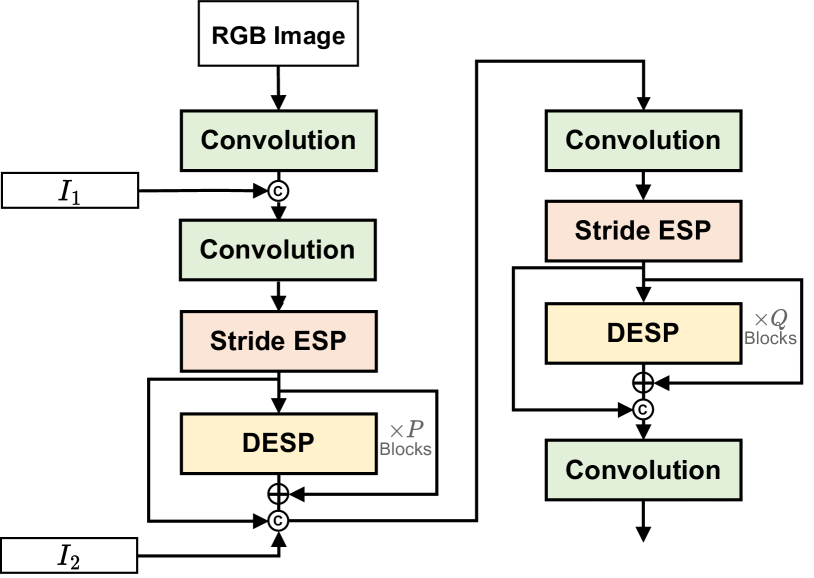
Figure 3: Comprehensive Schematic of the Encoder in Our Proposed Model

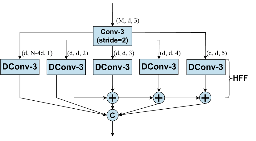
(a) Stride ESP

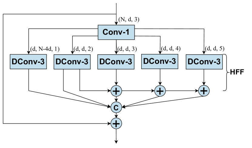
(b) ESP

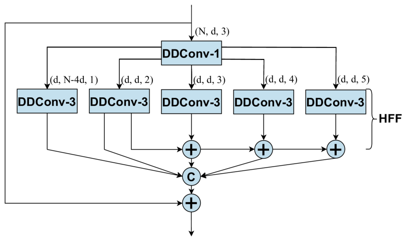
(c) DESP

Figure 4: This figure presents the ESP blocks within the Encoder. The convolutional layers are designated as Conv-n (standard $n\times n$ convolution), DConv-n ($n\times n$ dilated convolution), and DDConv-n ($n\times n$ depthwise dilated convolution), and are described in terms of $(input$ $channels,$ $output$ $channels,$ $dilation$ $rate)$. These blocks consolidate feature maps employing a Hierarchical Feature Fusion (HFF)[13], which is notable for its computational efficiency and its ability to eliminate grid-like artifacts resulting from dilated convolutions. The Stride ESP (a) not only accomplishes downsampling but also converts the depth of the feature map from $M$ to $N$, whereas ESP (Fig 4(b)) and DESP (Fig 4(c)) maintain the original dimensions of the feature map.

3.2 Decoder

In our TwinLiteNet⁺ architecture, we implement an innovative approach by deploying multiple decoding modules, each tailored for a distinct segmentation task. This design deviates from conventional methods that typically depend on a singular output for all object categories, with the tensor output encompassing $C+1$ channels, corresponding to $C$ classes and one additional channel for the background. Specifically, the post-processing feature map obtained from PCAA denoted as $\textbf{F}_{pcaa}\in\mathbb{R}^{C\times\frac{H}{8}\times\frac{W}{8}}$, our architecture employs two separate yet structurally identical decoding blocks. These blocks independently handle the segmentation of distinct regions and drivable lanes. Our decoder effectively reduces the depth of the feature map and employs upsampling techniques. The upsampling process within the decoder is facilitated by a combination of Transpose Convolution and Convolution operations. We introduce two novel blocks, namely the Upper Convolution Block (UCB) and Upper Simple Block (USB), both elegantly designed for upsampling purposes. The UCB comprises a Transpose Convolution followed by two subsequent Convolution operations, wherein the post-Transpose Convolution features are concatenated with the input image at a lower resolution, either I₁ or I₂. Conversely, the USB incorporates a single Transpose Convolution and one Convolution, without merging input image information, and its output constitutes the segment map as predicted by the model. We apply batch normalization and PReLU following each Transpose Convolution or Convolution layer. Integrating a Convolution layer immediately subsequent to a Transpose Convolution significantly enhances the feature learning capabilities of the Decoder, thereby facilitating the restoration of resolution lost during the downsampling process in the encoder. The detailed architecture of our model’s Decoder Block is depicted in Figure 5. We have strategically designed our decoder to be simplistic, thereby ensuring minimal computational overhead for the model. The sequential application of the blocks $UCB\to UCB\to USB$ leads to a systematic change in the feature map dimensions from $\frac{H}{8}\times\frac{W}{8}\to\frac{H}{4}\times\frac{W}{4}\to\frac{H}{2}\times\frac{W}{2}\to H\times W$ for each targeted task. This modular, branched approach allows for the independent tuning of each task, facilitating the creation of optimal conditions for refining specific segmentation outcomes for various regions and drivable lanes. As a result, our model adeptly discriminates and enhances features relevant to each segmentation task, culminating in an output resolution of $\textbf{O}\in\mathbb{R}^{2\times H\times W}$.

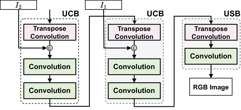
Figure 5: Decoder Block Design in TwinLiteNet⁺. This illustrates the implementation of Upper Convolution Block (UCB) and Upper Simple Block (USB) within the decoder, specifically tailored for upsampling to generate segment maps for diverse tasks.

3.3 Model configurations

Our TwinLiteNet⁺ model is configured into four distinct variants: TwinLiteNet⁺-nano, TwinLiteNet⁺-small, TwinLiteNet⁺-medium, and TwinLiteNet⁺-large, with TwinLiteNet⁺-large being the largest variant comprising 1.94M parameters, and TwinLiteNet⁺-nano the smallest with only 0.03M parameters. The models differ in terms of the number of kernels in convolutional layers and the hyperparameters P and Q, while retaining the overall architecture. The specifics of these configurations are detailed in Table 1. This leads to variations in the number of parameters and computational costs across the variants. The development of these four variants demonstrates our model’s versatility across different configurations and opens up options for deployment on diverse hardware platforms. This versatility is particularly significant for embedded devices, enabling the inference capabilities of the TwinLiteNet⁺ model, especially in the TwinLiteNet⁺-nano version with its 0.03M parameters and a computational requirement of 0.57 GFLOPs.

3.4 Loss Function

In the design of our proposed segmentation model, we incorporate two distinct loss functions: Focal Loss [34] and Tversky Loss [35]. These functions are chosen to tackle specific challenges in pixel-wise classification tasks effectively.

Focal Loss [34]: Focal Loss is designed to address pixel classification errors by focusing more on misclassified samples. It modifies the standard cross-entropy loss to emphasize hard-to-predict samples, thereby improving performance in imbalanced datasets. The function is defined in Eq. 5. Where $N$ is the total number of pixels, $C$ is the number of classes, $\hat{p}$ is the predicted probability of pixel $i$ for class $c$, $p_{i}(c)$ is the ground truth, and $\gamma$ is a parameter that adjusts the focus on difficult samples.

$$\mathcal{L}_{focal}=-\frac{1}{N}\sum_{c=0}^{C-1}\sum_{i=1}^{N}p_{i}(c)(1-\hat{p}_{i}(c))^{\gamma}\log(\hat{p}_{i}(c))$$ (5)

Tversky Loss [35]: An adaptation of Dice Loss [38], Tversky Loss addresses class imbalances in segmentation tasks by introducing parameters $\alpha$ and $\beta$ to control the impact of false positives and false negatives which is detailed in Eq. 6. where $TP$, $FN$, and $FP$ are the counts of true positives, false negatives, and false positives, respectively. The parameters $\alpha$ and $\beta$ allow fine-tuning the loss to emphasize precision or recall, making it a versatile tool for handling imbalanced data in segmentation tasks.

$$\mathcal{L}_{tversky}=\sum_{c=0}^{C}(1-\frac{TP(c)}{TP(c)+\alpha FN(c)+\beta FP(c)})$$ (6)

The overall loss function, which aggregates the contributions from both Focal and Tversky Losses, is formulated for each segmentation head as:

$$\begin{split}\mathcal{L}=\mathcal{L}_{\text{drivable}}+\mathcal{L}_{\text{lane}}\end{split}$$ (7)

where $\mathcal{L}_{\text{drivable}}$ and $\mathcal{L}_{\text{lane}}$ represent the aggregated Focal and Tversky Losses for Drivable Area and Lane segmentation, respectively.

Table 1: Model architecture configuration

Layer	Ouput Size	Output channels for TwinLiteNet+
		Nano	Small	Medium	Large
Conv	$\frac{H}{2}\times\frac{W}{2}$	4	8	16	32
Conv		8	16	32	64
Stride ESP	$\frac{H}{4}\times\frac{W}{4}$	16	32	64	128
P $\times$ DESP		16	32	64	128
Conv		32	64	128	256
Stride ESP	$\frac{H}{8}\times\frac{W}{8}$	32	64	128	256
Q $\times$DESP		32	64	128	256
Conv		16	32	64	128
PCAA		16	32	64	128
Conv		8	16	32	64
UCB${}_{\text{drivable}}$ UCB${}_{\text{lane}}$	$\frac{H}{4}\times\frac{W}{4}$	4	8	16	32
UCB${}_{\text{drivable}}$ UCB${}_{\text{lane}}$	$\frac{H}{2}\times\frac{W}{2}$	4	8	8	8
UCB${}_{\text{drivable}}$ UCB${}_{\text{lane}}$	$H\times W$	2	2	2	2
P, Q		1, 1	2, 3	3, 5	5, 7
#Param.		0.03M	0.12M	0.48M	1.94M
FLOPs		0.57G	1.40G	4.63G	17.58G

4 Experimental

4.1 Experiment Details

4.1.1 Dataset

The BDD100K [39] dataset was used for training and validating TwinLiteNet⁺. With 100,000 frames and annotations for 10 tasks, it is a large dataset for autonomous driving. Due to its diversity in geography, environment, and weather conditions, the algorithm trained on the BDD100K dataset is robust enough to generalize to new settings. The BDD100K dataset is divided into three parts: a training set with 70,000 images, a validation set with 10,000 images, and a test set with 20,000 images. Since no labels are available for the 20,000 images in the test set, we chose to evaluate on a separate validation set of 10,000 images. We used data prepared similarly to several previous studies [4, 8, 10] to ensure fairness in comparison.

Algorithm 2 TwinLiteNet⁺ Training Stage

1:Target end-to-end network $F$ with parameters $\Theta$; Training dataset $\tau_{train}$; Validation dataset $\tau_{val}$

2:Well-trained network: $F(x;\Theta)$

3:Initialize the parameters $\Theta$

4:for epoch: 1 $\rightarrow$ epochs do

5:     for each batch $(x_{train},y_{train})$ in $\tau_{train}$ do

6:         $y_{\text{drivable}},y_{\text{lane}}\leftarrow y_{train}$

7:         $\hat{y}_{\text{drivable}},\hat{y}_{\text{lane}}\leftarrow F(x_{train})$

8:         $\mathcal{L}_{\text{drivable}}\leftarrow\mathcal{L}_{\text{drivable}}^{focal}(y_{\text{drivable}},\hat{y}_{\text{drivable}})$

9:…………………..$\quad+\mathcal{L}_{\text{drivable}}^{tversky}(y_{\text{drivable}},\hat{y}_{\text{drivable}})$

10:         $\mathcal{L}_{\text{lane}}\leftarrow\mathcal{L}_{\text{lane}}^{focal}(y_{\text{lane}},\hat{y}_{\text{lane}})$

11:…………………..$\quad+\mathcal{L}_{\text{lane}}^{tversky}(y_{\text{lane}},\hat{y}_{\text{lane}})$

12:         $\mathcal{L}\leftarrow\mathcal{L}_{\text{drivable}}+\mathcal{L}_{\text{lane}}$

13:         $\Theta\leftarrow{\arg\!\min}_{\Theta}\mathcal{L}$

14:         $\Theta\leftarrow{\text{Update}}_{\text{EMA}}\Theta$

15:     end for

16:     $x_{val},y_{val}\leftarrow\tau_{val}$

17:     $\hat{y}_{val}\leftarrow F(x_{val})$

18:     $mIoU_{\text{drivable}}\leftarrow Evaluate(\hat{y}_{val},y_{val})$

19:     $Acc_{\text{lane}},IoU_{\text{lane}}\leftarrow Evaluate(\hat{y}_{val},y_{val})$

20:end for

21:return $F(x;\Theta)$

4.1.2 Evaluation Metrics

For the segmentation tasks, similar to the evaluation approach in [10, 11, 29], we assess the drivable area segmentation task using the mIoU (mean Intersection of Union) metric. In the context of lane segmentation, we gauge performance using both accuracy and IoU (Intersection over Union) metrics. However, owing to pixel imbalances between the background and foreground in lane segmentation, we opt for a more meaningful balanced accuracy metric in our evaluation. Traditional accuracy metrics may produce biased results by favoring classes with a larger number of samples. In contrast, balanced accuracy provides a fairer assessment by considering the accuracy for each class. We used the accuracy metrics provided in the study [11]. All experiments used the PyTorch framework on an NVIDIA GeForce RTX A5000 GPU with 32GB of RAM and an Intel(R) Core(TM) i9-10900X processor.

4.1.3 Experimental Setup and Implementation

To improve performance, we apply several data augmentation techniques. To address photometric distortions, we modify the hue, saturation, and value parameters of the image. In addition, we also incorporate basic enhancement techniques to handle geometric distortions such as random translation, cropping, and horizontal flipping. We train our model using the AdamW optimizer with a learning rate of $5\times 10^{-4}$, momentum of 0.9, and weight decay of $5\times 10^{-4}$. In our TwinLiteNet⁺ we use EMA (Exponential Moving Average) model [40] purely as the final inference model. Additionally, we resize the original image dimensions from 1280 × 720 to 640 × 384. For the loss function coefficients, we set $\alpha$ = 0.7 and $\beta$ = 0.3 for $\mathcal{L}_{drivable}^{tversky}$, $\alpha$ = 0.9 and $\beta$ = 0.1 for $\mathcal{L}_{lane}^{tversky}$, and $\alpha_{t}$ = 0.25 and $\gamma$ = 2 in $\mathcal{L}_{da,ll}^{focal}$. All of the specified configurations are developed based on empirical evidence. Finally, we conduct training with a batch size of 16 on an RTX A5000 for 100 epochs. The model training process is described in Algorithm LABEL:train. During the model training process, we simultaneously train both tasks and employ EMA technique for weight updates following each backpropagation step. After each epoch, we evaluate the model on the validation set and focus on three key metrics: mean Intersection over Union for the Drivable Area Segmentation task (mIoU_drivable), Lane Accuracy, and Intersection over Union for the Lane Segmentation task (Acc_l, IoU_l).

Table 2: Calculation results for the cost of the TwinLiteNet⁺ model with various versions. Parameters and FLOPs represent the number of parameters and the amount of computation. Latency for inference with different batch sizes.

Model	FPS (with Batch Size) $\uparrow$					#Param. $\downarrow$	FLOPs $\downarrow$ (batch=1)	Model Size $\downarrow$
	1	2	4	8	16
TwinLiteNet${}^{+}_{\text{Nano}}$	237	470	921	1004	1163	0.03M	0.57G	0.06MB
TwinLiteNet${}^{+}_{\text{Small}}$	178	340	697	732	779	0.12M	1.40G	0.23MB
TwinLiteNet${}^{+}_{\text{Medium}}$	138	269	442	456	484	0.48M	4.63G	0.92MB
TwinLiteNet${}^{+}_{\text{Large}}$	109	186	218	220	237	1.94M	17.58G	3.72MB

4.2 Experimental results

4.2.1 Cost Computation Performance

Table 2 presents the computational cost outcomes of various versions of the TwinLiteNet⁺ model. The parameters include the number of parameters ($\#$Param.), and FLOPs indicating the computation required per inference (with a batch size of 1), along with the model’s size. Frame rate (FPS) is measured across different batch sizes (1, 2, 4, 8, 16) to assess latency during inference. Results show that TwinLiteNet${}^{+}_{\text{Nano}}$ is the lightest version with only 0.03M parameters and 0.57G FLOPs, achieving an impressive inference speed of up to 1163 FPS with a batch size of 16. Inference with larger batch sizes opens up the potential for simultaneous inference across multiple cameras, a critical capability for autonomous vehicle applications. However, transitioning from the Nano to the Large version, the parameters surge to 1.94M and FLOPs to 17.58G, indicating a more powerful computational capability but also increased latency, with inference speed dropping to 237 FPS. The trade-off between accuracy and latency is evident: larger models offer higher computational potential but require more processing time. This highlights the importance of carefully balancing the need for accuracy and real-time requirements when selecting a model for specific applications.

Table 3: Performance Benchmarking of Drivable Area and Lane Segmentation Models

Model	Drivable Area		Lane		FLOPS $\downarrow$	#Param. $\downarrow$
	mIoU (%) $\uparrow$		Accuracy (%) $\uparrow$	IoU (%) $\uparrow$
DeepLabV3+ [41] (’18)	90.9		–	29.8	30.7G	15.4M
SegFormer [42] (’21)	92.3		–	31.7	12.1G	7.2M
R-CNNP [10] (’22)	90.2		–	24.0	–	–
YOLOP [10] (’22)	91.6		–	26.5	8.11G	5.53M
IALaneNet (ResNet-18) [7] (’23)	90.54		–	30.39	89.83G	17.05M
IALaneNet (ResNet-34) [7] (’23)	90.61		–	30.46	139.46G	27.16M
IALaneNet (ConvNeXt-tiny) [7] (’23)	91.29		–	31.48	96.52G	18.35M
IALaneNet (ConvNeXt-small) [7] (’23)	91.72		–	32.53	200.07G	39.97M
YOLOv8(multi) [43] (’23)	84.2		81.7	24.3	–	–
Sparse U-PDP [44] (’23)	91.5		–	31.2	–	–
TwinLiteNet [8] (’23)	91.3		77.8	31.1	3.9G	0.44M
TwinLiteNet${}^{+}_{\text{Nano}}$	87.3		70.2	23.3	0.57G	0.03M
TwinLiteNet${}^{+}_{\text{Small}}$	90.6		75.8	29.3	1.40G	0.12M
TwinLiteNet${}^{+}_{\text{Medium}}$	92.0		79.1	32.3	4.63G	0.48M
TwinLiteNet${}^{+}_{\text{Large}}$	92.9		81.9	34.2	17.58G	1.94M

Groundtruth

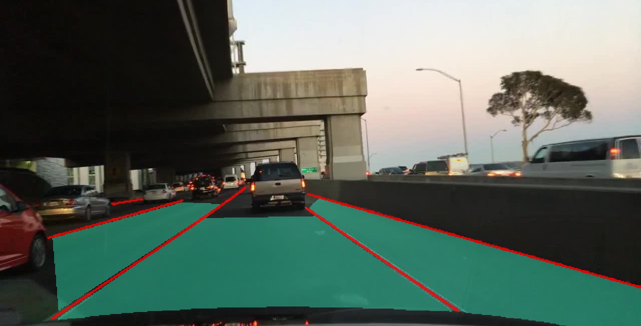
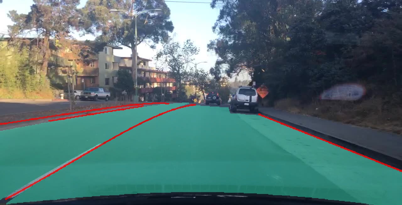
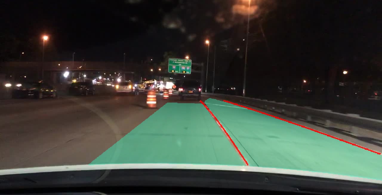
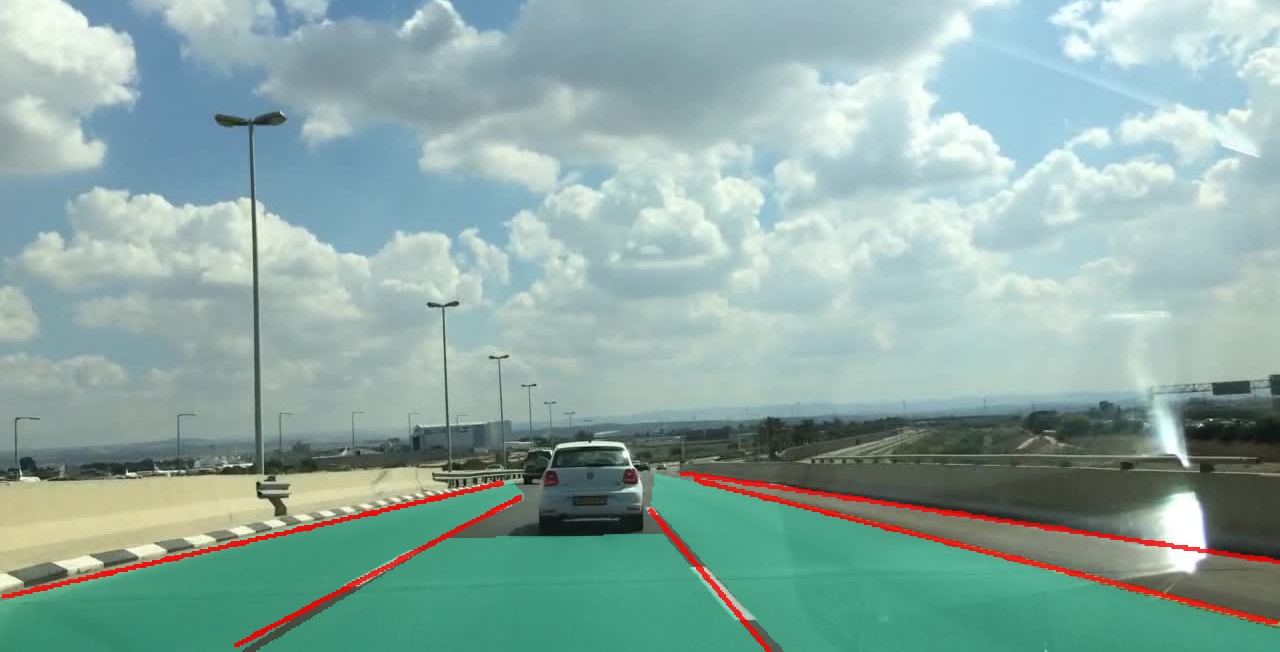
TwinLiteNet

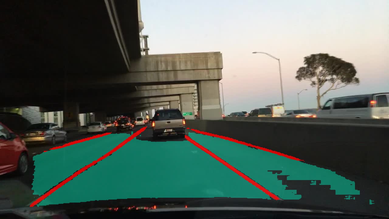
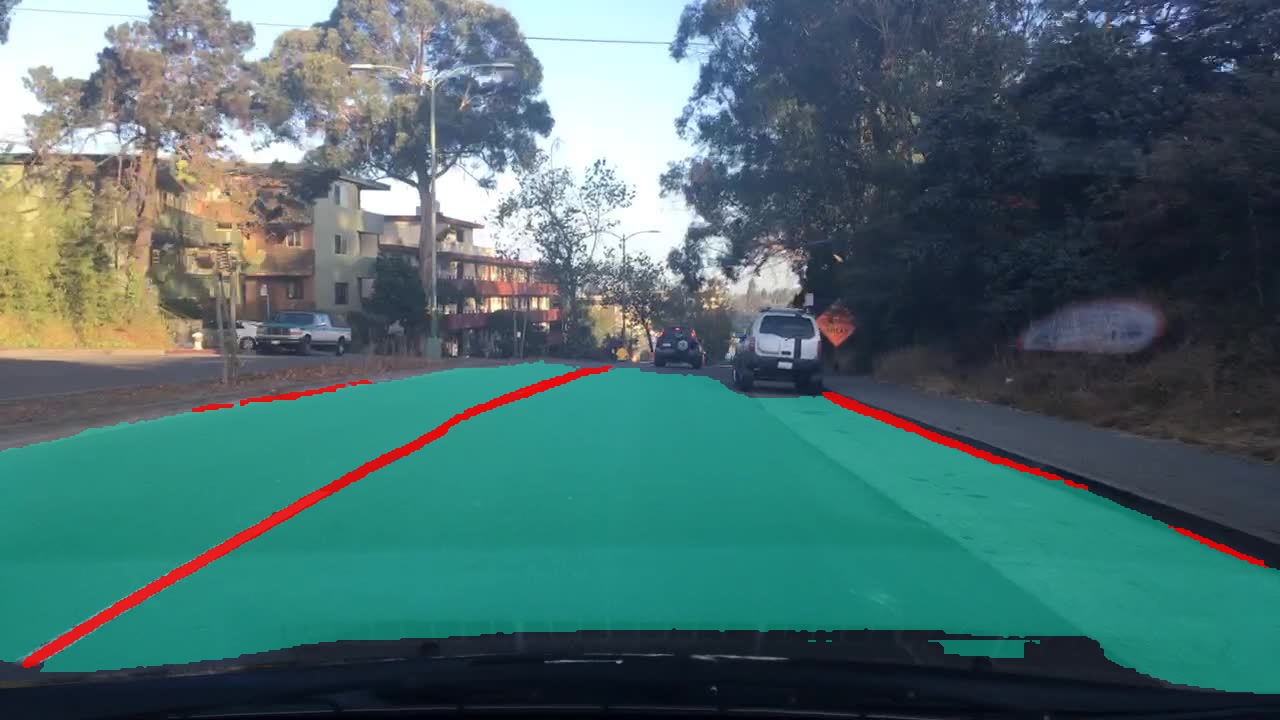
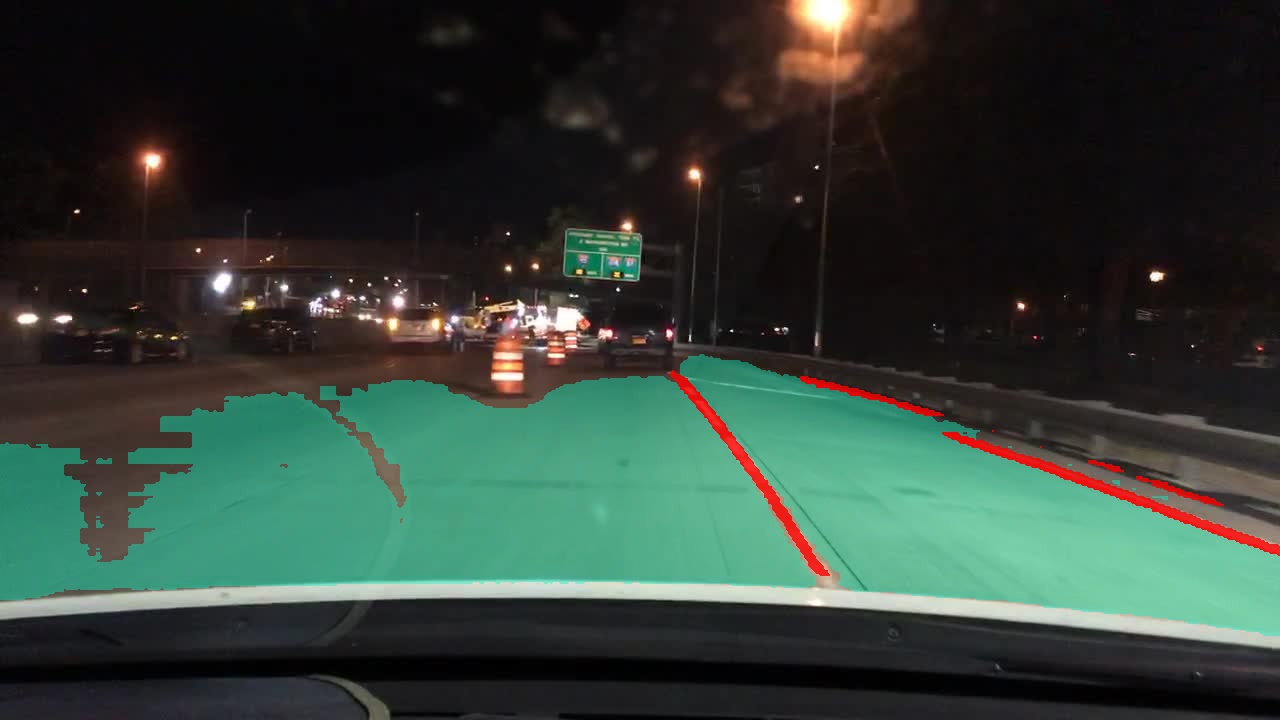
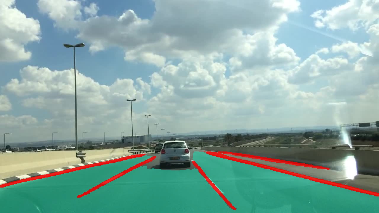
TwinLiteNet⁺ Large

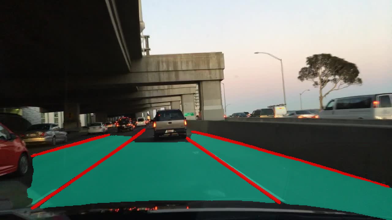
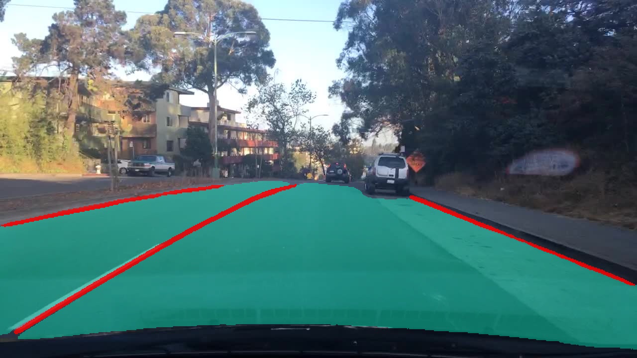
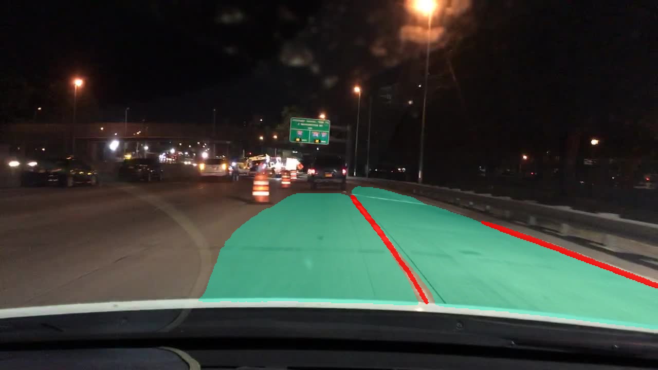
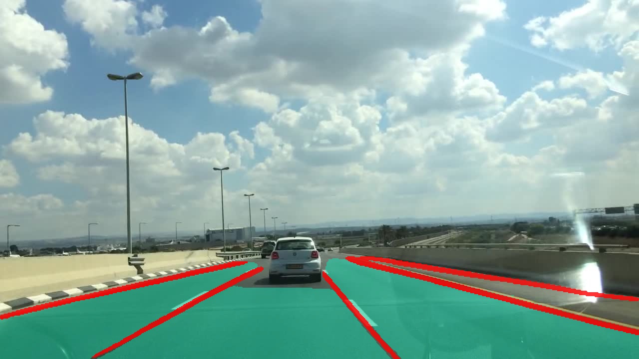
TwinLiteNet⁺ Medium

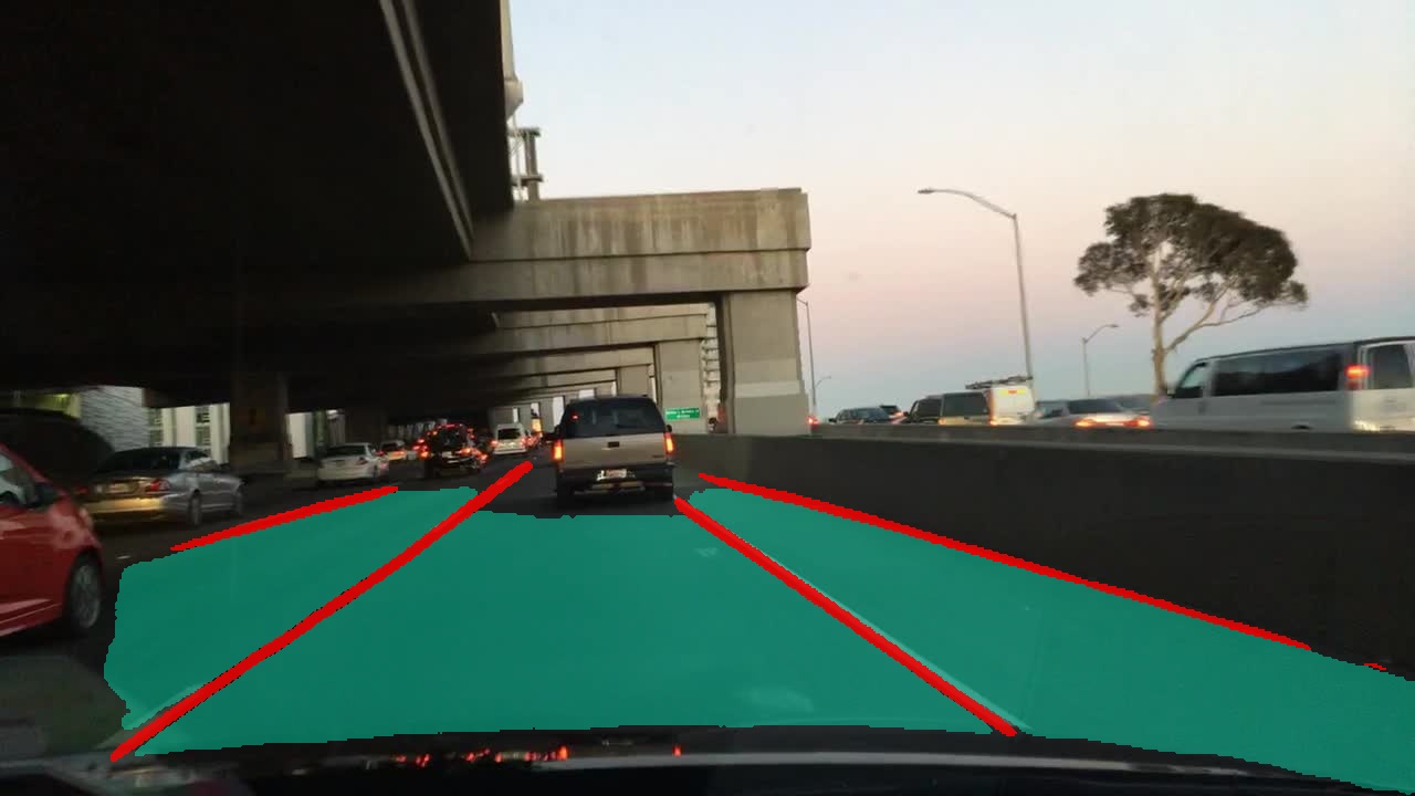
TwinLiteNet⁺ Small

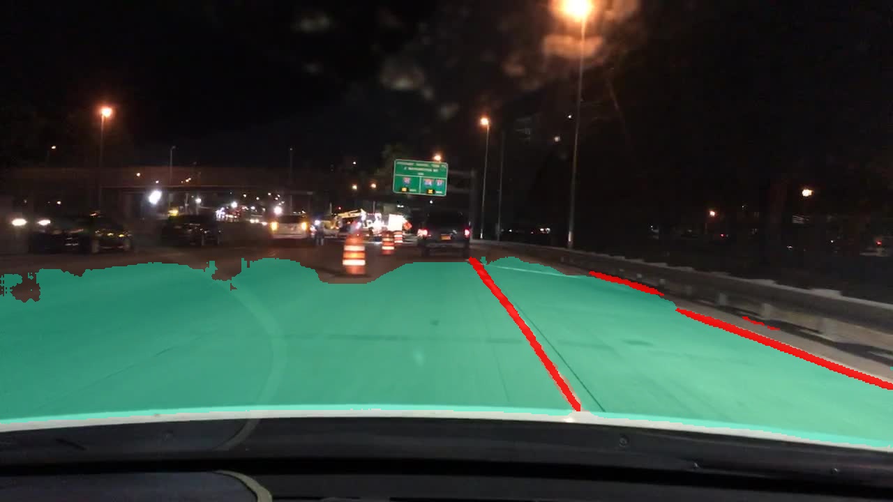
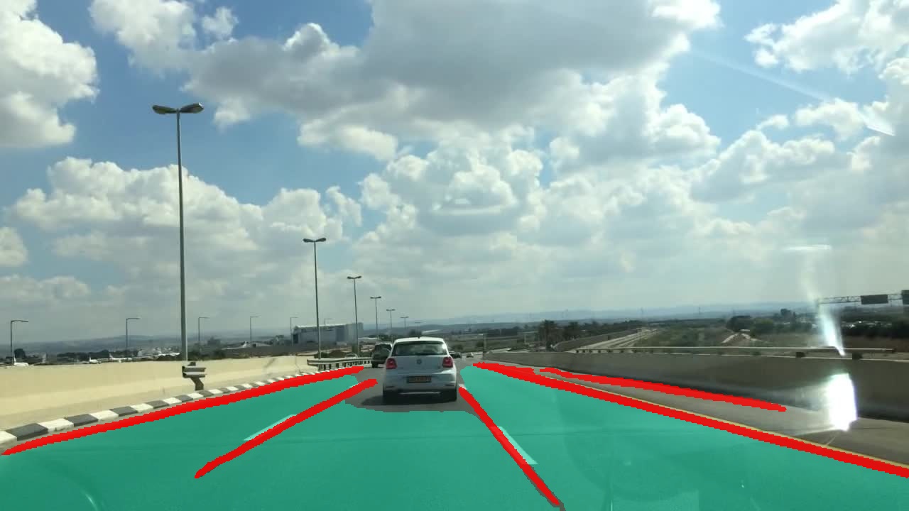
TwinLiteNet⁺
Nano

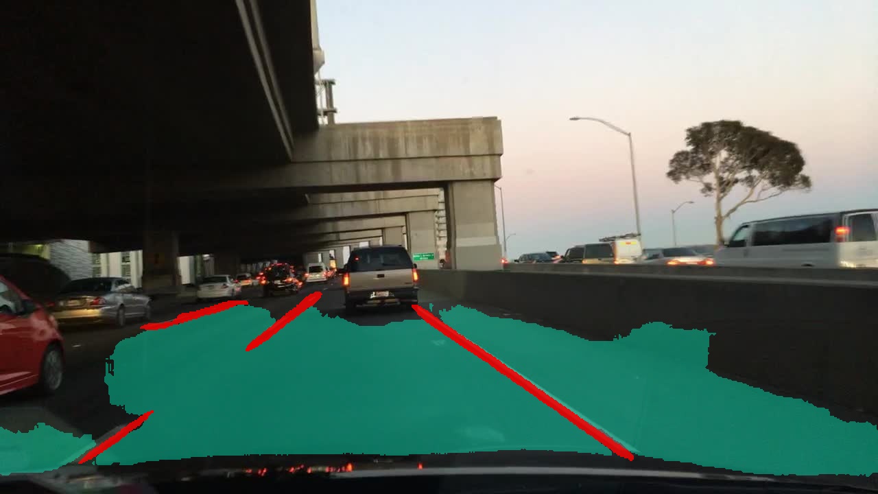
(a)

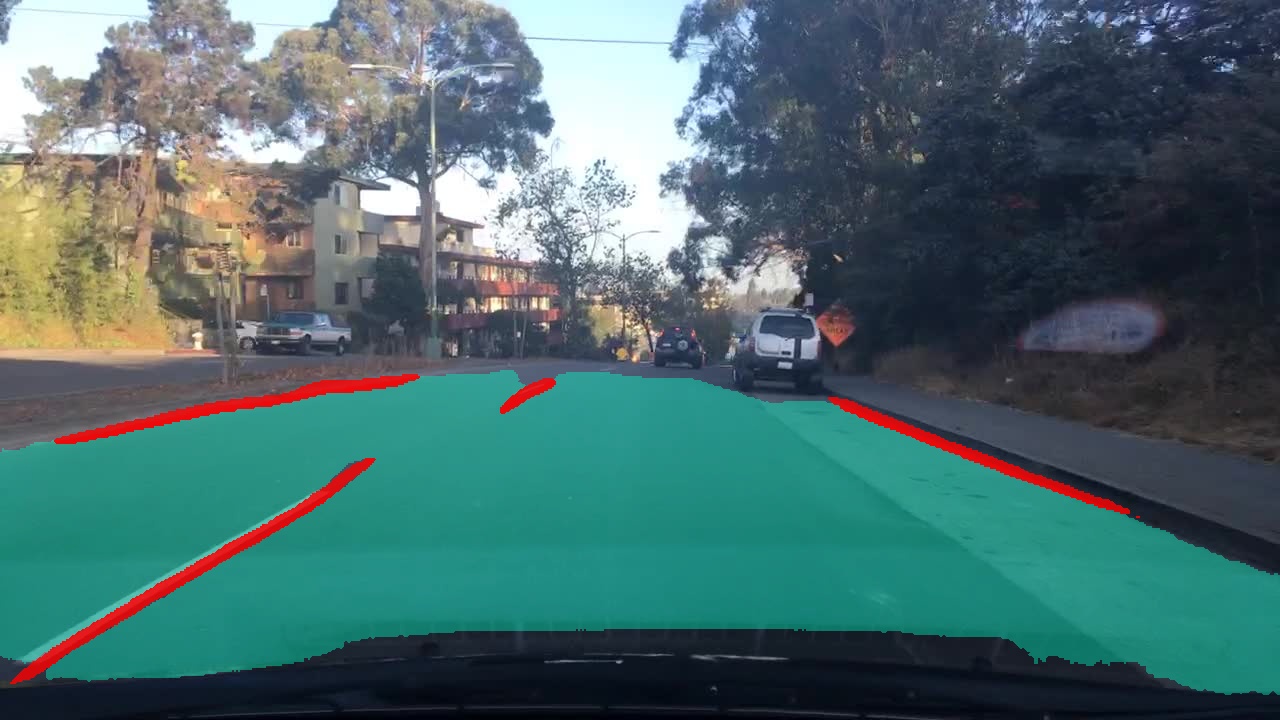
(b)

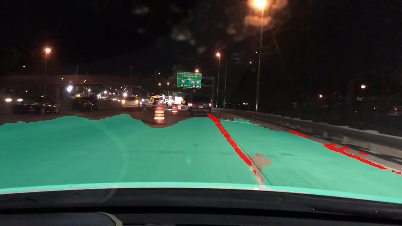
(c)

(d)

Figure 6: Drivable Area and Lane Segmentation comparison results

4.2.2 Drivable Area Segmentation & Lane Detection Result

In this section, we will proceed to compare our models with other models that undertake the same tasks of drivable area segmentation and lane detection. To ensure fairness, we will not compare with single-task models or models that perform an additional task such as object detection. All our experimental results in this section are presented in Fig 1 and Table 3. The provided table offers a comprehensive overview of the performance of models in drivable area segmentation and lane detection. The TwinLiteNet⁺ models, particularly the Nano, Small, and Medium versions, stand out for their lightweight architecture and high-speed performance. Despite TwinLiteNet${}^{+}_{\text{Nano}}$ achieving only about 87.3% mIoU, it has the lowest requirements with just 0.57G FLOPS and 0.03M parameters. The larger versions, like TwinLiteNet${}^{+}_{\text{Medium}}$ and Large, significantly improve mIoU and lane detection IoU, with TwinLiteNet${}^{+}_{\text{Large}}$ reaching 92.9% mIoU and 34.2% IoU, surpassing all current models and nearing top-tier performance while still maintaining optimal parameter and FLOPS usage. Other models like DeepLabV3+, SegFormer, and YOLOP also perform well but require more resources. This highlights the advantage of TwinLiteNet⁺ in terms of performance and resource efficiency. Notably, TwinLiteNet${}^{+}_{\text{Large}}$ not only improves in mIoU but also accuracy and IoU for lane detection, achieving the highest levels compared to other models. Overall, the table demonstrates the trade-off between performance and resource utilization. While larger models like TwinLiteNet${}^{+}_{\text{Large}}$ offer high performance, smaller ones like Nano and Small have the advantage of speed and low resource requirements, suitable for applications needing quick and efficient responses. These results provide critical information for researchers and engineers when selecting and optimizing models for practical applications. We visually compare the TwinLiteNet⁺ with the TwinLiteNet model. We evaluate the performance of the model not only in daylight conditions but also at night. As we are concerned, intense sunlight or low-light environments can affect the driver’s visibility. Similarly, it impacts the model’s performance. This poses challenges for the performance of drivable area and lane segmentation. In Figure 6, the various variants of TwinLiteNet⁺ are compared to their predecessor, TwinLiteNet, in the two tasks of drivable area and lane segmentation. Overall, the TwinLiteNet${}^{+}_{\text{Large}}$ and TwinLiteNet${}^{+}_{\text{Medium}}$ models perform significantly better than the basic TwinLiteNet, showing superior architecture and excelling in handling complex road constructions and diverse environmental conditions. As seen in Figure 6(b) and Figure 6(c), TwinLiteNet shows more misclassified regions and unclear boundaries compared to a more consistent and accurate delineation of roads of the aforementioned. Conversely, our ultra-lightweight model versions designed for situations with limited computational resources did not perform as expected in complex road structures, however, still reflect an effort in recognizing lanes and roads as in Figure 6(c) and Figure 6(d).

(a) Ground truth
.
.

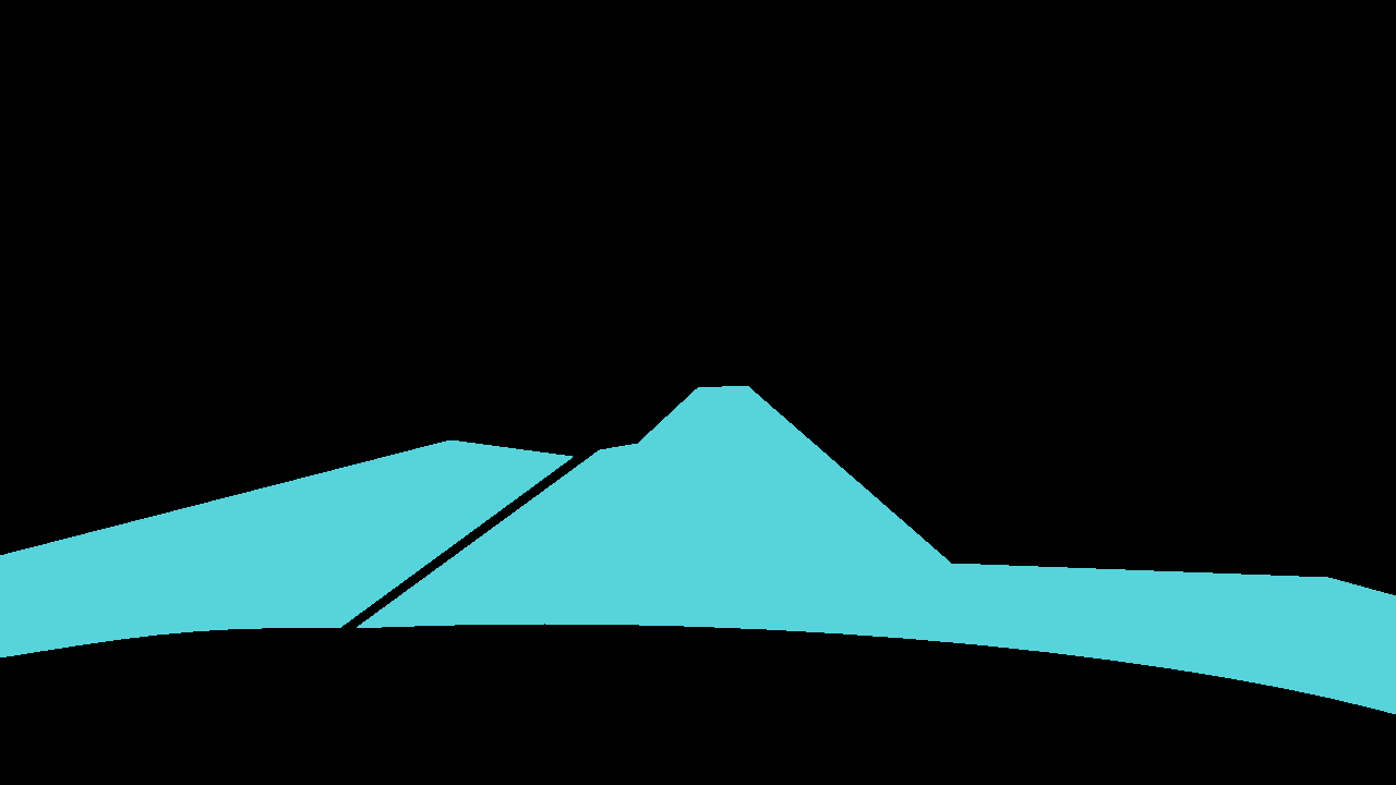
(b) Drivable Area Segmentation

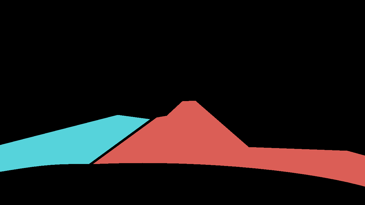
(c) Directly & Alternative Area segmentation

Figure 7: Examples of Directly & Alternative Area segmentation task.

4.2.3 Directly $\&$ Alternative Area segmentation results

In this study, we extend our investigations to a model addressing the segmentation of directly and alternatively drivable areas. This approach contrasts with standard drivable area segmentation, which typically conflates these two distinct zones into a single category. Figure 7 illustrates the main difference between the two segmentation tasks in Fig 7(b) and Fig 7(c), with the latter distinctly segmenting directly & alternative area, Red regions are directly drivable. The separated segmentation of these two areas enables vehicles to differentiate between precisely navigable regions and alternative paths, facilitating lane changes or maneuvers around obstacles in the directly drivable area. When implementing this segmentation, the drivable area segmentation decoder block output has three channels instead of two. Consequently, the model’s output are $\textbf{O}_{drivable}\in\mathbb{R}^{3\times H\times W}$ and $\textbf{O}_{lane}\in\mathbb{R}^{2\times H\times W}$, reflecting the enhanced detection capabilities. Table 4 provides a comprehensive and detailed overview of the performance of various segmentation models applied to direct region segmentation and replacement. In addition to the evaluation of the Mean Intersection over Union (mIoU), in this study, we also assess the Pixel Accuracy (PA) and Mean Pixel Accuracy (mPA), facilitating comparison with previous research. In this experiment, we compare the TwinLiteNet${}^{+}_{\text{Large}}$ model after modifications to demonstrate the responsiveness of our model to this task, and we name it as TwinLiteNet${}^{+}_{\text{D\&A}}$ to differentiate it from the Large one. Additionally, we experiment with the TwinLiteNet${}^{+}_{\text{D\&A}}$ model when performing multi-tasks and the TwinLiteNet${}^{+}_{\text{D\&A}}$ with only one decoding block for the driving area segmentation. Notably, the IBN-NET model from 2020 demonstrates a significant improvement in mIoU, indicating its robustness in capturing intricate area details compared to its predecessors. The TwinLiteNet${}^{+}_{\text{D\&A}}$ models, in both multitask and single-task configurations, stand out with high performance across all three metrics, with our TwinLiteNet${}^{+}_{\text{D\&A}}$ model achieving the highest mPA of 92.1%, surpassing previous studies. This comprehensive assessment underscores the advancements in segmentation techniques and highlights the TwinLiteNet${}^{+}_{\text{D\&A}}$ model’s potential to improve accuracy and detail capture in image segmentation tasks. We present some results of the TwinLiteNet${}^{+}_{\text{D\&A}}$ model in Figure 8 to emphasize its proficiency in differentiating between directly drivable and alternative paths under various lighting conditions, from daylight to nighttime scenarios.

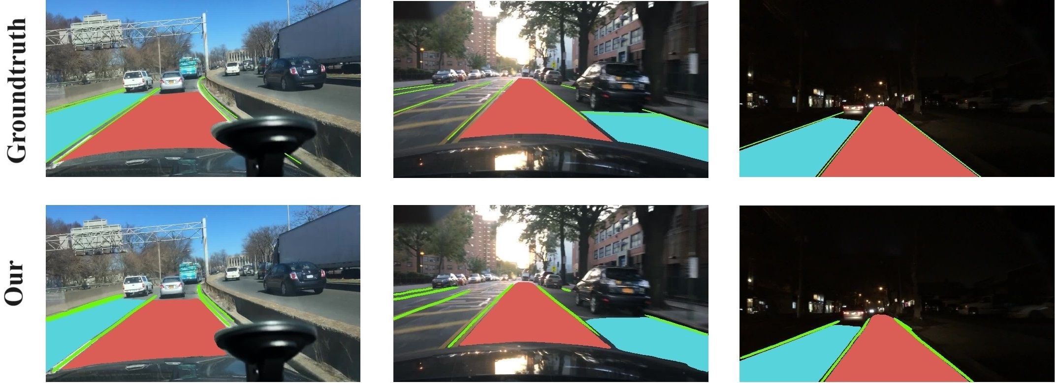
Figure 8: Some results of the multi-task model. Red regions are directly drivable, the blue ones are alternative and the lanes are green.

Table 4: Segmentation model results for Directly & Alternative Area segmentation

Model	Multitask	Directly & Alternative Area
		mIoU (%) $\uparrow$	PA(%) $\uparrow$	mPA(%) $\uparrow$
[45] (’19)	✘	82.62	–	–
ShuDA-RFBNet [46] (’19)	✘	82.67	–	–
IBN-NET [47] (’20)	✘	86.16	–	–
RN101+ASPP+FPN[17] (’21)	✘	84.58	97.09	91.14
RN101+FPN[17] (’21)	✘	82.70	96.51	91.42
RN101+ASPP+top-down[17] (’21)	✘	82.80	96.60	90.68
RN101+top-down[17] (’21)	✘	82.44	96.24	88.39
DeepLabv3+[41] (’18)	✘	84.73	–	–
[28] (’21)	✔	83.34	–	–
[48] (’22)	✘	83.01	–	–
IDS-MODEL [49] (’23)	✘	83.63	–	–
TwinLiteNet${}^{+}_{\text{D\&A}}$	✘	83.9	96.9	92.0
	✔	84.3	97.0	92.1

Table 5: Comparative Analysis of TwinLiteNet${}^{+}_{\text{Large}}$ in Different Environmental Settings

Photometric scene		Number	Drivable Area		Lane
			mIoU (%)		IoU (%)
Weather conditions	Clear	5,346	93.1		33.8
	Overcast	1,239	93.7		35.8
	Undefined	1,157	93.2		35.4
	Snowy	769	91.6		31.6
	Rainy	738	90.2		32.0
	Partly Cloudy	738	93.3		35.3
	Foggy	13	92.4		29.6
Periods of day	Daytime	5,258	93.2		35.1
	Night	3,929	92.5		32.9
	Dawn/Dusk	778	92.9		33.9
	Undefined	35	86.7		29.3
Traffic scenes	City street	6,112	92.8		34.4
	Highway	2,499	93.3		33.8
	Residential	1,253	92.8		34.4
	Undefined	53	90.3		31.0
	Parking lot	49	88.1		25.1
	Tunnel	27	89.8		28.9
	Gas station	7	88.8		14.2

Table 6: Performance Metrics of the TwinLiteNet⁺ Across Quantization Approaches

	Drivable Area				Lane
	mIoU (%)				Accuracy (%)				IoU (%)
	FP32	FP16	INT8		FP32	FP16	INT8		FP32	FP16	INT8
			PTSQ	QAT			PTSQ	QAT			PTSQ	QAT
TwinLiteNet${}^{+}_{\text{Nano}}$	87.3	87.3 $\downarrow$ 0.0	86.0 $\downarrow$ 1.3	86.9 $\downarrow$ 0.4	70.2	70.1 $\downarrow$ 0.1	67.2 $\downarrow$ 3.0	69.9 $\downarrow$ 0.3	23.3	23.2 $\downarrow$ 0.1	21.8 $\downarrow$0.5	23.2 $\downarrow$0.1
TwinLiteNet${}^{+}_{\text{Small}}$	90.6	90.6 $\downarrow$ 0.0	88.5 $\downarrow$ 2.1	90.2 $\downarrow$ 0.4	75.8	75.7 $\downarrow$ 0.1	74.6 $\downarrow$ 1.2	75.6 $\downarrow$ 0.2	29.3	29.3 $\downarrow$ 0.0	28.3 $\downarrow$1.0	28.8 $\downarrow$0.5
TwinLiteNet${}^{+}_{\text{Medium}}$	92.0	92.0 $\downarrow$ 0.0	91.6 $\downarrow$ 0.4	91.9 $\downarrow$ 0.1	79.1	79.1 $\downarrow$ 0.0	77.1 $\downarrow$ 2.0	78.6 $\downarrow$ 0.5	32.3	32.2 $\downarrow$0.1	31.5 $\downarrow$0.8	31.9 $\downarrow$0.4
TwinLiteNet${}^{+}_{\text{Large}}$	92.9	92.9 $\downarrow$ 0.0	92.7 $\downarrow$ 0.2	92.7 $\downarrow$ 0.2	81.9	81.9 $\downarrow$ 0.0	80.2 $\downarrow$ 1.7	81.4 $\downarrow$ 0.5	34.2	34.2 $\downarrow$ 0.0	33.6 $\downarrow$0.6	34.0 $\downarrow$0.2

4.2.4 Panoptic driving perception results

The BDD100K dataset encompasses a vast collection of annotations for weather conditions, periods of day, and various scenes, ranging from urban streets and expansive highways to residential neighborhood areas. This dataset’s distribution mirrors the diverse content found in images, offering a rich landscape for exploration in image domain adaptation. This eclectic mix of images serves as a compelling avenue for research in the context of self-driving vehicles. Consequently, we embark on a thorough quantitative assessment of our TwinLiteNet⁺ variants, evaluating their adaptability and performance across distinct environmental contexts and scenarios. The results presented in Table 5 demonstrate that our model, TwinLiteNet⁺, exhibits proficient inference capabilities across diverse environments and conditions. These findings underscore the model’s adaptability and generalization ability in various conditions and scenarios related to autonomous driving applications.

Table 7: TwinLiteNet⁺ Model Results: Multitasking Learning versus Single-Task Learning

Method	Drivable Area		Lane		Parameter $\downarrow$	GFLOPs $\downarrow$
	mIoU (%) $\uparrow$		Acc (%) $\uparrow$	IoU (%) $\uparrow$
Drivable (only)	92.6		–	–	1.91M	16.97
Lane (only)	–		81.9	34.4	1.91M	16.97
Multi-task	92.9 $\uparrow$ 0.3		81.9 $\downarrow$ 0.0	34.2 $\downarrow$ 0.2	1.94M $\uparrow$ 0.03	17.58 $\uparrow$ 0.61

Table 8: Results of the TwinLiteNet⁺ Model with different experimental settings

Tversky Loss	Multiple Decoder	PCAA	EMA	Drivable Area		Lane		#Param.	GFLOPs
				mIoU (%)		Acc (%)	IoU (%)
✘	✘	✘	✘	91.2		78.1	25.9	1.84M	16.83
✔	✘	✘	✘	91.3 $\uparrow$ 0.1		80.9 $\uparrow$ 2.8	29.3 $\uparrow$ 3.4	1.84M $\uparrow$ 0.00	16.83 $\uparrow$ 0.00
✔	✔	✘	✘	92.4 $\uparrow$ 1.2		81.2 $\uparrow$ 3.1	33.5 $\uparrow$ 7.6	1.87M $\uparrow$ 0.03	17.42 $\uparrow$ 0.59
✔	✔	✔	✘	92.7 $\uparrow$ 1.5		81.7 $\uparrow$ 3.6	33.9 $\uparrow$ 8.0	1.94M $\uparrow$ 0.1	17.5 $\uparrow$ 0.67
✔	✔	✔	✔	92.9 $\uparrow$ 1.7		81.9 $\uparrow$ 3.8	34.2 $\uparrow$ 8.3	1.94M $\uparrow$ 0.1	17.5 $\uparrow$ 0.67

4.3 Deployment

Table 9: Comparative Analysis of Latency and Power Consumption on Embedded Devices

	Version	Jetson Xavier	Jetson TX2
Latency (ms)	Nano	9.1550 $\pm$ 0.092	22.268 $\pm$ 0.156
	Small	12.861 $\pm$ 0.941	33.818 $\pm$ 0.134
	Medium	20.460 $\pm$ 0.067	61.785 $\pm$ 0.015
	Large	43.089 $\pm$ 0.198	153.24 $\pm$ 0.094
Power (Watt)	Nano	10.029 $\pm$ 2.267	3.647 $\pm$ 0.637
	Small	11.086 $\pm$ 2.385	4.043 $\pm$ 0.463
	Medium	13.585 $\pm$ 1.832	4.496 $\pm$ 0.202
	Large	15.980 $\pm$ 1.187	4.883 $\pm$ 0.057

To demonstrate the practical applicability of our TwinLiteNet⁺ model on hardware with limited computational capabilities, we conducted experiments using various inference data types, including Floating Point 32-bit (FP32), Floating Point 16-bit (FP16), and Integer 8-bit (INT8). For the INT8 data type, we employed quantization techniques, specifically Post-Training Static Quantization (PTSQ) and Quantization-Aware Training (QAT). With QAT, instead of training the model from scratch, we leveraged the pre-trained technique and implemented QAT over 10 epochs. Table 6 demonstrates that TwinLiteNet⁺ maintains impressive performance using different quantization methods. Notably, the Quantization-Aware Training technique significantly mitigates the performance degradation commonly seen when transitioning from FP32 to INT8, which is crucial for applications with limited computational capabilities. The slight reduction in accuracy for tasks like drivable area and lane segmentation indicates a balance between accuracy and computational efficiency. Furthermore, we implemented our model on several embedded devices such as Jetson Xavier and Jetson TX2. We used TensorRT-FP16 for inference and then measured the inference latency and power consumption on each device. To minimize measurement discrepancies, we conducted five iterations of measurements for each test. Results from Table 9 show that using the TwinLiteNet⁺ model on embedded devices like Jetson Xavier and Jetson TX2 yields promising results in terms of inference latency and power consumption. Specifically, the Nano and Small versions of the model exhibited low latency and reasonable power consumption on both devices, highlighting the model’s performance optimization capability in a limited computational environment. Although the Medium and Large versions have higher latency and power consumption, they still maintain an acceptable level, demonstrating the model’s flexibility and scalability. These results not only validate the impressive performance of TwinLiteNet⁺ but also underscore its practical potential in real-world applications, particularly in the field of autonomous vehicles and smart embedded systems.

Table 10: More comparison: The best and second best results are marked in bold and underline respectively.

Model	Drivable Area		Lane	Params $\downarrow$
	mIoU (%) $\uparrow$		IoU (%) $\uparrow$
Drivable Area Segmentation (Only)
PSPNet [1] (’17)	89.6		–	–
MultiNet [2] (’18)	71.6		–	–
R-CNNP (DA-Seg) [10] (’22)	90.2		–	–
YOLOP (DA-Seg) [10] (’22)	92.0		–	–
MFIALane (DA) [5] (’22)	91.9		–	–
YOLOv8 (segda) [43] (’23)	78.1		–	–
Lane Segmentation (Only)
ENet [12] (’16)	–		14.64	–
SCNN [3] (’17)	–		15.84	–
ENET-SAD [4] (’19)	–		16.02	–
MFIALane (LL) [5] (’22)	–		37.9	–
YOLOv8 (segll) [43] (’23)	–		22.9	–
Drivable Area and Lane Segmentation
DeepLabV3+ [41] (’18)	90.9		29.8	15.4M
SegFormer [42] (’21)	92.3		31.7	7.2M
JSU [6] (’22)	92.68		26.92	–
R-CNNP [10] (’22)	90.2		24.0	–
YOLOP (Seg only) [10] (’22)	91.6		26.5	5.53M
IALaneNet (ConvNeXt-small) [7] (’23)	91.72		32.53	39.97M
YOLOv8 (multi) [43] (’23)	84.2		24.3	–
Sparse U-PDP (w/o detection) [44] (’23)	91.5		31.2	–
TwinLiteNet [8] (’23)	91.3		31.1	0.44M
Drivable Area and Lane Segmentation + Vehicle Detection
HybridNets [9] (’22)	90.5		31.6	13.8M
YOLOP (Multitask) [10] (’22)	91.5		26.2	7.9M
DRMNet [50] (’23)	92.2		27	8.09M
DP-YOLO [51] (’23)	91.5		26.0	8.7M
YOLOPv2 [29] (’23)	93.2		27.25	38.9M
A-YOLOM(n) [11] (’23)	90.5		28.2	4.43
A-YOLOM(s) [11] (’23)	91.0		28.8	13.61
YOLOPX [52] (’23)	93.2		27.2	32.9M
CenterPNets [30] (’23)	92.8		32.1	28.56
Sparse U-PDP [44] (’23)	92.9		32.4	12.05
TwinLiteNet${}^{+}_{\text{Nano}}$	87.3		23.3	0.03M
TwinLiteNet${}^{+}_{\text{Small}}$	90.6		29.3	0.12M
TwinLiteNet${}^{+}_{\text{Medium}}$	92.0		32.3	0.48M
TwinLiteNet${}^{+}_{\text{Large}}$	92.9		34.2	1.94M

4.4 Ablation study

To assess the impact of the multitasking approach on each task, we compared the performance of the TwinLiteNet${}^{+}_{\text{Large}}$ model in multitasking against its performance in executing each task separately after removing irrelevant decoders. The TwinLiteNet${}^{+}_{\text{Large}}$(Drivable only) specializes in segmenting drivable areas, while the TwinLiteNet${}^{+}_{\text{Large}}$(Lane only) focuses on lane segmentation. The results, presented in Table 7, show that employing multitask learning not only improves the mIoU for the task of segmenting drivable areas (by an increase of 0.2%), but also leads to certain trade-offs. Specifically, while there’s a slight increase in performance for drivable area segmentation task, the IoU for the lane segmentation task decreases by 0.2% when multitasking, and simultaneously, the model size and computational cost also increase, respectively, by 0.03M and 0.61 GFLOPs.

We have undertaken numerous modifications and enhancements, along with extensive experimentation. Table 8 presents a curated list of changes implemented during our experiments and the corresponding improvements integrated into the entire network, culminating in a potent segmentation model for drivable areas and lanes. We constructed a Baseline model comprising an Encoder block and a single Decoder block for both tasks, as opposed to two Decoder blocks. The output of this Baseline model is now $\textbf{O}\in\mathbb{R}^{3\times H\times W}$, encompassing three channels: two for the segmentation tasks and one for the background. Our Baseline does not utilize Partial Class Activation Attention, instead directly concatenating the Encoder and Decoder blocks. During training, this Baseline solely employs Focal Loss for error computation and does not utilize Exponential Moving Average (EMA). Sequentially, we augmented the Baseline with Tversky Loss, Multiple Decoder, Partial Class Activation Attention, and EMA. The results demonstrate significant improvements in both segmentation tasks due to our proposed methods. Specifically, with the full implementation of these enhancements, the model exhibited an increase in mIoU for drivable area segmentation from 90.9% to 92.9% and an increase in IoU for lane segmentation from 25.2% to 34.2%. This not only proves the efficacy of each component but also illustrates the power of their combination. Although there is a slight increase in model size and computational cost, these improvements have contributed to setting a new standard in segmentation performance for practical applications.

4.5 More comparison

In this section, we will compare the TwinLiteNet⁺ model with all models including single-task models and multitask models encompassing segmentation and object detection tasks. In section 4.4, we demonstrated that either single-task or multitask execution could improve accuracy, so it is not surprising that some results indicate our model’s accuracy is lower than some single-task models or those incorporating object detection. Upon examining the numerical data in Table 10, it’s evident that the TwinLiteNet⁺ models demonstrate a competitive performance across different configurations. While the TwinLiteNet${}^{+}_{\text{Nano}}$ shows modest performance with the lowest parameters, highlighting its potential for lightweight applications, the TwinLiteNet${}^{+}_{\text{Large}}$ model achieves impressive results, especially in lane segmentation with an IoU of 34.2% and drivable area segmentation with a mIoU of 92.9%, outperforming many other models. This indicates that while our model may not always surpass single-task models in individual tasks, it provides a balanced and efficient solution for multitask scenarios. Notably, when compared to other models that perform both drivable area and lane segmentation along with vehicle detection, TwinLiteNet${}^{+}_{\text{Large}}$ shows a commendable blend of high accuracy and relatively lower parameter count, suggesting an efficient trade-off between performance and model complexity. These insights underline the efficacy of our model in handling complex, real-world scenarios that require simultaneous perception tasks.

5 Conclusion

In this study, we introduce TwinLiteNet⁺, a novel model that enhances drivable area segmentation and lane detection capabilities, and demonstrates efficient deployment on embedded devices. Designed to optimize the balance between accuracy and computational efficiency, the model is configurable across a spectrum from Nano to Large variants to accommodate diverse requirements. Experimental evaluations reveal that TwinLiteNet⁺ not only achieves superior accuracy on the BDD100K dataset but also exhibits versatile deployment potential on devices with constrained computational power. This work pioneers a novel approach for the development of intelligent driving and driver assistance systems, underscoring the importance of AI model optimization for real-world deployment. TwinLiteNet⁺ signifies a stride forward in enhancing performance and inference speed, heralding a new era in AI applications within the autonomous driving domain and contributing to the advancement of safety and efficiency on the roads.

References

- [1] H. Zhao, J. Shi, X. Qi, X. Wang, J. Jia, Pyramid scene parsing network, in: Proceedings of the IEEE Conference on Computer Vision and Pattern Recognition (CVPR), 2017.
- [2] M. Teichmann, M. Weber, M. Zöllner, R. Cipolla, R. Urtasun, Multinet: Real-time joint semantic reasoning for autonomous driving, in: 2018 IEEE Intelligent Vehicles Symposium (IV), 2018, pp. 1013–1020. doi:10.1109/IVS.2018.8500504.
- [3] A. Parashar, M. Rhu, A. Mukkara, A. Puglielli, R. Venkatesan, B. Khailany, J. S. Emer, S. W. Keckler, W. J. Dally, Scnn: An accelerator for compressed-sparse convolutional neural networks, 2017 ACM/IEEE 44th Annual International Symposium on Computer Architecture (ISCA) (2017) 27–40.
- [4] Y. Hou, Z. Ma, C. Liu, C. C. Loy, Learning lightweight lane detection cnns by self attention distillation, 2019 IEEE/CVF International Conference on Computer Vision (ICCV) (2019) 1013–1021.
- [5] Z. Qiu, J. Zhao, S. Sun, Mfialane: Multiscale feature information aggregator network for lane detection, IEEE Transactions on Intelligent Transportation Systems 23 (12) (2022) 24263–24275. doi:10.1109/TITS.2022.3195742.
- [6] D.-G. Lee, Y.-K. Kim, Joint semantic understanding with a multilevel branch for driving perception, Applied Sciences 12 (2022) 2877. doi:10.3390/app12062877.
- [7] W. Tian, X. Yu, H. Hu, Interactive attention learning on detection of lane and lane marking on the road by monocular camera image, Sensors 23 (14) (2023).
- [8] Q.-H. Che, D.-P. Nguyen, M.-Q. Pham, D.-K. Lam, Twinlitenet: An efficient and lightweight model for driveable area and lane segmentation in self-driving cars, in: 2023 International Conference on Multimedia Analysis and Pattern Recognition (MAPR), 2023, pp. 1–6. doi:10.1109/MAPR59823.2023.10288646.
- [9] D. Vu, B. Ngo, H. Phan, Hybridnets: End-to-end perception network (2022). arXiv:2203.09035.
- [10] D. Wu, M.-W. Liao, W.-T. Zhang, X. Wang, X. Bai, W. Cheng, W.-Y. Liu, Yolop: You only look once for panoptic driving perception, Machine Intelligence Research 19 (2021) 550 – 562.
- [11] J. Wang, Q. M. J. Wu, N. Zhang, You only look at once for real-time and generic multi-task (2023). arXiv:2310.01641.
- [12] A. Paszke, A. Chaurasia, S. Kim, E. Culurciello, Enet: A deep neural network architecture for real-time semantic segmentation, ArXiv abs/1606.02147 (2016).
- [13] S. Mehta, M. Rastegari, A. Caspi, L. Shapiro, H. Hajishirzi, Espnet: Efficient spatial pyramid of dilated convolutions for semantic segmentation, in: V. Ferrari, M. Hebert, C. Sminchisescu, Y. Weiss (Eds.), Computer Vision – ECCV 2018, Springer International Publishing, Cham, 2018, pp. 561–580.
- [14] S. Mehta, M. Rastegari, L. Shapiro, H. Hajishirzi, Espnetv2: A light-weight, power efficient, and general purpose convolutional neural network, in: 2019 IEEE/CVF Conference on Computer Vision and Pattern Recognition (CVPR), 2019, pp. 9182–9192. doi:10.1109/CVPR.2019.00941.
- [15] J. Fu, J. Liu, H. Tian, Y. Li, Y. Bao, Z. Fang, H. Lu, Dual attention network for scene segmentation, in: 2019 IEEE/CVF Conference on Computer Vision and Pattern Recognition (CVPR), 2019, pp. 3141–3149. doi:10.1109/CVPR.2019.00326.
- [16] S.-A. Liu, H. Xie, H. Xu, Y. Zhang, Q. Tian, Partial class activation attention for semantic segmentation, in: Proceedings of the IEEE/CVF Conference on Computer Vision and Pattern Recognition, 2022.
- [17] D. Qiao, F. Zulkernine, Drivable area detection using deep learning models for autonomous driving, in: 2021 IEEE International Conference on Big Data (Big Data), 2021, pp. 5233–5238. doi:10.1109/BigData52589.2021.9671392.
- [18] V. Ostankovich, R. Yagfarov, M. Rassabin, S. Gafurov, Application of cyclegan-based augmentation for autonomous driving at night, in: 2020 International Conference Nonlinearity, Information and Robotics (NIR), 2020, pp. 1–5. doi:10.1109/NIR50484.2020.9290218.
- [19] A. Chaurasia, E. Culurciello, Linknet: Exploiting encoder representations for efficient semantic segmentation, in: 2017 IEEE Visual Communications and Image Processing (VCIP), 2017, pp. 1–4. doi:10.1109/VCIP.2017.8305148.
- [20] K.-Y. Chiu, S.-F. Lin, Lane detection using color-based segmentation, in: IEEE Proceedings. Intelligent Vehicles Symposium, 2005., 2005, pp. 706–711. doi:10.1109/IVS.2005.1505186.
- [21] T.-Y. Sun, S.-J. Tsai, V. Chan, Hsi color model based lane-marking detection, in: 2006 IEEE Intelligent Transportation Systems Conference, 2006, pp. 1168–1172. doi:10.1109/ITSC.2006.1707380.
- [22] J. Wang, Y. Ma, S. Huang, T. Hui, F. Wang, C. Qian, T. Zhang, A keypoint-based global association network for lane detection, in: CVPR, 2022.
- [23] Q. Qiu, H. Gao, W. Hua, G. Huang, X. He, Priorlane: A prior knowledge enhanced lane detection approach based on transformer, in: 2023 IEEE International Conference on Robotics and Automation (ICRA), 2023, pp. 5618–5624. doi:10.1109/ICRA48891.2023.10161356.
- [24] Y. Ko, Y. Lee, S. Azam, F. Munir, M. Jeon, W. Pedrycz, Key points estimation and point instance segmentation approach for lane detection, IEEE Transactions on Intelligent Transportation Systems 23 (7) (2022) 8949–8958. doi:10.1109/TITS.2021.3088488.
- [25] Z. Qin, P. Zhang, X. Li, Ultra fast deep lane detection with hybrid anchor driven ordinal classification, IEEE Transactions on Pattern Analysis and Machine Intelligence (2022) 1–14doi:10.1109/TPAMI.2022.3182097.
- [26] H. Honda, Y. Uchida, Clrernet: Improving confidence of lane detection with laneiou (2023). arXiv:2305.08366.
- [27] F. Pizzati, F. García, Enhanced free space detection in multiple lanes based on single cnn with scene identification, in: 2019 IEEE Intelligent Vehicles Symposium (IV), 2019, pp. 2536–2541. doi:10.1109/IVS.2019.8814181.
- [28] D.-G. Lee, Fast drivable areas estimation with multi-task learning for real-time autonomous driving assistant, Applied Sciences 11 (22) (2021). doi:10.3390/app112210713.
- [29] C. Han, Q. Zhao, S. Zhang, Y. Chen, Z. Zhang, J. Yuan, Yolopv2: Better, faster, stronger for panoptic driving perception (2022). arXiv:2208.11434.
- [30] G. Chen, T. Wu, J. Duan, Q. Hu, D. Huang, H. Li, Centerpnets: A multi-task shared network for traffic perception, Sensors 23 (5) (2023). doi:10.3390/s23052467.
- [31] A. Howard, M. Zhu, B. Chen, D. Kalenichenko, W. Wang, T. Weyand, M. Andreetto, H. Adam, Mobilenets: Efficient convolutional neural networks for mobile vision applications (04 2017).
- [32] X. Jiang, H. Wang, Y. Chen, Z. Wu, L. Wang, B. Zou, Y. Yang, Z. Cui, Y. Cai, T. Yu, C. Lv, Z. Wu, Mnn: A universal and efficient inference engine, in: MLSys, 2020.
- [33] S.-A. Liu, H. Xie, H. Xu, Y. Zhang, Q. Tian, Partial class activation attention for semantic segmentation, in: 2022 IEEE/CVF Conference on Computer Vision and Pattern Recognition (CVPR), 2022, pp. 16815–16824. doi:10.1109/CVPR52688.2022.01633.
- [34] T.-Y. Lin, P. Goyal, R. Girshick, K. He, P. Dollar, Focal loss for dense object detection, in: Proceedings of the IEEE International Conference on Computer Vision (ICCV), 2017.
- [35] S. S. M. Salehi, D. Erdogmus, A. Gholipour, Tversky loss function for image segmentation using 3d fully convolutional deep networks, in: Q. Wang, Y. Shi, H.-I. Suk, K. Suzuki (Eds.), Machine Learning in Medical Imaging, Springer International Publishing, Cham, 2017, pp. 379–387.
-
[36]
S. Ioffe, C. Szegedy, Batch normalization: Accelerating deep network training by reducing internal covariate shift, CoRR abs/1502.03167 (2015).
arXiv:1502.03167.
URL http://arxiv.org/abs/1502.03167 -
[37]
K. He, X. Zhang, S. Ren, J. Sun, Delving deep into rectifiers: Surpassing human-level performance on imagenet classification, CoRR abs/1502.01852 (2015).
arXiv:1502.01852.
URL http://arxiv.org/abs/1502.01852 - [38] C. H. Sudre, W. Li, T. Vercauteren, S. Ourselin, M. Jorge Cardoso, Generalised dice overlap as a deep learning loss function for highly unbalanced segmentations, in: Deep Learning in Medical Image Analysis and Multimodal Learning for Clinical Decision Support, Springer International Publishing, Cham, 2017, pp. 240–248.
- [39] F. Yu, H. Chen, X. Wang, W. Xian, Y. Chen, F. Liu, V. Madhavan, T. Darrell, Bdd100k: A diverse driving dataset for heterogeneous multitask learning, in: 2020 IEEE/CVF Conference on Computer Vision and Pattern Recognition (CVPR), 2020, pp. 2633–2642. doi:10.1109/CVPR42600.2020.00271.
- [40] A. Tarvainen, H. Valpola, Mean teachers are better role models: Weight-averaged consistency targets improve semi-supervised deep learning results, in: I. Guyon, U. V. Luxburg, S. Bengio, H. Wallach, R. Fergus, S. Vishwanathan, R. Garnett (Eds.), Advances in Neural Information Processing Systems, Vol. 30, Curran Associates, Inc., 2017.
- [41] L.-C. Chen, Y. Zhu, G. Papandreou, F. Schroff, H. Adam, Encoder-decoder with atrous separable convolution for semantic image segmentation, in: V. Ferrari, M. Hebert, C. Sminchisescu, Y. Weiss (Eds.), Computer Vision – ECCV 2018, Springer International Publishing, Cham, 2018, pp. 833–851.
- [42] E. Xie, W. Wang, Z. Yu, A. Anandkumar, J. M. Alvarez, P. Luo, Segformer: Simple and efficient design for semantic segmentation with transformers, in: Neural Information Processing Systems (NeurIPS), 2021.
-
[43]
G. Jocher, A. Chaurasia, J. Qiu, Ultralytics YOLO (Jan. 2023).
URL https://github.com/ultralytics/ultralytics - [44] H. Wang, M. Qiu, Y. Cai, L. Chen, Y. Li, Sparse u-pdp: A unified multi-task framework for panoptic driving perception, IEEE Transactions on Intelligent Transportation Systems 24 (10) (2023) 11308–11320. doi:10.1109/TITS.2023.3273286.
- [45] F. Pizzati, F. Garcia, Enhanced free space detection in multiple lanes based on single cnn with scene identification, in: 2019 IEEE Intelligent Vehicles Symposium (IV), IEEE, 2019. doi:10.1109/ivs.2019.8814181.
- [46] Z. Wang, Z. Cheng, H. Huang, J. Zhao, Shuda-rfbnet for real-time multi-task traffic scene perception, in: 2019 Chinese Automation Congress (CAC), 2019, pp. 305–310. doi:10.1109/CAC48633.2019.8997236.
- [47] X. Pan, P. Luo, J. Shi, X. Tang, Two at once: Enhancing learning and generalization capacities via ibn-net, in: V. Ferrari, M. Hebert, C. Sminchisescu, Y. Weiss (Eds.), Computer Vision – ECCV 2018, Springer International Publishing, Cham, 2018, pp. 484–500.
- [48] L. Sun, F. Yan, T. Deng, C. Jiang, J. Li, A lightweight network with lane feature enhancement for multilane drivable area detection, in: 2022 14th International Conference on Wireless Communications and Signal Processing (WCSP), 2022, pp. 66–71.
- [49] T. Luo, Y. Chen, T. Luan, B. Cai, L. Chen, H. Wang, Ids-model: An efficient multi-task model of road scene instance and drivable area segmentation for autonomous driving, IEEE Transactions on Transportation Electrification (2023) 1–1doi:10.1109/TTE.2023.3293495.
- [50] J. Zhao, D. Wu, Z. Yu, Z. Gao, Drmnet: A multi-task detection model based on image processing for autonomous driving scenarios, IEEE Transactions on Vehicular Technology (2023) 1–16doi:10.1109/TVT.2023.3296735.
- [51] X. Zeng, Y. Qi, M. Liu, Multi-task panoramic driving perception algorithm based on improved yolov5, Highlights in Science, Engineering and Technology 34 (2023) 314–325. doi:10.54097/hset.v34i.5489.
- [52] J. Zhan, Y. Luo, C. Guo, Y. Wu, J. Meng, J. Liu, Yolopx: Anchor-free multi-task learning network for panoptic driving perception, Pattern Recognition 148 (2024) 110152.