unicode breaklinks=true citecolor=blue See front_cut_v2.pdf

pageanchor=false

DOCTORAL THESIS at Charles University

Jakub Podgorný

Polarisation properties of X-ray emission from accreting supermassive black holes

Astronomical Institute of Charles University, Astronomical
Institute of the Czech Academy of Sciences, Strasbourg astronomical observatory

Supervisors of the doctoral thesis: RNDr. Michal Dovčiak, Ph.D.
Dr. Frédéric Marin Study programme at Charles University: Theoretical Physics, Astronomy and Astrophysics Study branch at Charles University: P4F1

Prague and Strasbourg 2023

See correction_notice.pdf

pageanchor=true I declare that I carried out this doctoral thesis independently, and only with the cited sources, literature and other professional sources. It has not been used to obtain another or the same degree. The content provided here, including all text and images, has been created without the use of any artificial intelligence tools. All material is the result of human creativity and effort.

I understand that my work relates to the rights and obligations under the Act No. 121/2000 Sb., the Copyright Act, as amended, in particular the fact that the Charles University has the right to conclude a license agreement on the use of this work as a school work pursuant to Section 60 subsection 1 of the Copyright Act.

In date   Author’s signature

A personal dedication

I have always tried to think of my work within the broadest possible terms. My use of references – as mentioned in the “Preface” – is not intended, therefore, either to be pretentious or to convey the impression that this dissertation carries greater weight than it actually does. Within any given lifetime – a lifetime being a characteristic human measure –, a period of three years’ work is one of considerable duration, though it amounts to almost nothing when considered from a collective viewpoint. I am extremely grateful that, whilst possessing only the limited knowledge of an early-career researcher, I have been given the opportunity to add my own particular pine needle to what is a growing and collectively assembled anthill. Besides attempting to make certain parts of my chosen endeavor useful to the local scientific community – as is only inevitable –, I have also sought to ensure that the work as a whole should serve my own personal purposes.

After familiarizing myself with the endless – though non-routine – cycle of initial insights and the ensuing development thereof through which results emerge and age, a choice of specialization had necessarily to be made. Although inquiry into the disciplines of physical cosmology, philosophy, (art) history, consciousness studies, or even mathematics, to cite several examples, might seem to offer a broader field of comprehension when it comes to providing a basis on which to generalize, it is my firm belief that, in fact, there does not exist any true hierarchy as far as areas of research are concerned, even in the case of astrophysics. Once a detailed and solvable problem has been identified, a problem which possesses high potential in terms of its capacity to be instructive, all that remains is for one to work, during the constructive phase, with every ounce of one’s passion and honesty, as well as in accordance with one’s particular capacities, the recognition of all of which has a calming effect upon oneself. Optimization. From disorder to order.

While acknowledging all of its unavoidable associated dubieties, I am nevertheless convinced that science is indeed soothing both to its practitioner and to society as a whole, inasmuch as it provides long-term, objective sureties, pace postmodernist trends of thought. I chose the field of numerical simulations of black-hole environments for the reason that, to the extent that basic research itself allows, I found the implications useful – in the event that such research should come to fruition – and the object of study satisfying – insofar as it made its way towards that fruition. Nevertheless, were I to have chosen any other phenomenon warranting the devotion of three years to its study, it might also, I believe, have provided me with just as much scope – rather than insight per se –, not to mention preparation for upcoming challenges. I consider the greatest benefits of doctoral studies to be the following: they offer a person the opportunity to analyze one very specific problem in the deepest manner available; they oblige that person to exercise an overall mastery of efficient working practices; and they enable that same person to move towards a more productive period of their life once the learning phase has reached its term, thereby enabling them creatively to explore the unknown.

A large part of my doctoral dissertation was conducted in Strasbourg – an imposing medieval town of many wonders – and, most importantly, within the flourishing environment of the observatory, a workplace for which I shall probably struggle to find an equal at any time in the future. A comparable part was undertaken in Prague, the place of my birth and a city to which I owe both the days of my youth and the majority of my schooling and university education. While spending much of the latter period in the Karlov district of Prague, I came to develop a sense of the genius loci associated with all the dark corners and pubs into which celebrated Czech and German writers – e.g. Jaroslav Hašek (1883–1923) and Egon Erwin Kisch (1885–1948) – must once have ventured. This genius loci also made its presence felt within the university libraries themselves, as well as its lecture halls and corridors, through all of which great thinkers, including none other than Albert Einstein (1879–1955), must have passed. These same streets, stairways and gardens had once been filled with revolutionary students, the effects of whom on 20^th-century (Czech) history is well known. The neighborhood of Karlov likewise contained – and continues to do so – the aged hospitals where many have taken both their final and their first steps, – as in the case of my most beloved grandmother, Margit, and my newborn niece, Olga – and where many continue to devote their energies to healing others – as does my inspirational sister, Gabriela.

I have always truly appreciated the degree of patience extended and of instruction freely given to me during such times by acknowledged authorities; and, accordingly, I feel obliged to make use of it by virtue of producing fruitful research and to share my own acquired learning with those less fortunate or younger than myself. Alongside many others, of course, a few teachers in particular laid down enduring paths of inspiration within my mind (for the sake of brevity here mentioned without their academic titles): Jakub Haláček, who convinced me to opt for physics on completion of my high school education; Milan Pokorný, who showed me the beauty and power of mathematics during my undergraduate studies; and Oldřich Semerák, who not only reiterated to me at graduate level that same beauty and power, as found in General Relativity, but who also guided me towards the realization that art is of equal importance to me as is science, and that many interesting possibilities arise at precisely those points where these two intersect. For the majority of the quotations presented here below, I am indebted to Oldřich and to Jiří Bičák, the latter being yet another distinguished figure who has exerted a considerable degree of influence upon me. I should like to offer my foremost acknowledgement, however, to my two supervisors, Michal Dovčiak and Frédéric Marin, who have shown incredible endurance, provided me with staggering levels of support throughout my PhD, and also offered crucial feedback on all of the results presented below. My personal thanks go to you. Having been able to join the IXPE team of NASA and, in that setting, to have seen in detail the work of the greatest exponents within our field, can only be classed as a once-in-a-lifetime experience. I should also like to register my appreciation of the contribution made by Marie Novotná, who lent me great assistance as regards the graphic components of this dissertation as well as producing a number of illustrations. Mention should also be made of Robert D. Hughes (Prague), who kindly revised the English within the current section (viz. “A personal dedication”), and Karolina Hughes, who translated the below quotation.

None of the above would have been possible, however, without the ongoing support of my family and friends. I am well aware of the privilege I have enjoyed in terms of the fact that my particular background has enabled me to conduct specialized studies for almost a full decade in relation to one subject alone, a period of time just long enough to enable me, with an adequate degree of professionalism, to make small, independent steps towards extending the boundaries of human knowledge. In particular, I should like to thank my mother, Yvetta, who has had to make many sacrifices as I travelled down my chosen path and who herself has successfully confronted so many obstacles. My thanks next go to my girlfriend, Marie, whose support through the final and most important stages of the entire process, enabled me to finish my formal education. No less do I express my gratitude towards the friends and colleagues I have been able to make at both of the abovementioned institutions, as well as towards the Magnesium group in Prague and my flatmates in Strasbourg – they all contributed towards the fact that the three years I spent studying amounted to an experience of the greatest intensity, one of significance to me as much in terms of personal as of professional growth. Yet, despite the repeated upheavals our world has seen during the period in question, it was nevertheless for me – it must be said thanks to them – a fun time. Lastly, I should like to offer my thanks to those who have already died, yet remain with us in spirit. Most importantly so to my grandparents, Miroslav, Ludmila and Jiří, who all left strong roots from which to branch forth; to my mother’s second husband, Václav, whose humor and wisdom still resonate in Podolí (a district of Prague); and to my own beloved father, Oleg, who can only have had the heart of a whale. I should like to devote this work to my Dad. And I hope that, despite his having left us so soon, his lingering presence remains somewhere near Vyšehrad Castle – a place that means a lot to our family – and that he is smiling with pride at the progress I have been making.

Vždy budou duchové…, kteří budou usilovat, aby spojenou mocí poznání a snů, vědy a poezie, vytvořili jednotný obraz vesmírného dění, jenž by stejně odpovídal věčnému prahnutí lidského ducha po harmonii a kráse, i žízni srdce po spravedlnosti.
[There shall always be spirits… who will strive, through the combined forces of knowledge and dreams, as of science and poetry, to create a unified image of cosmic events, (one) which might reflect not only the human spirit’s eternal longing for harmony and beauty, but also the heart’s thirst for justice.]

Otokar Březina [excerpt from a letter to Brno-based classical philologist František Novotný]

Název práce: Polarizace rentgenového záření akreujících supermasivních černých děr

Autor: Jakub Podgorný

Ústav: Astronomický ústav Univerzity Karlovy, Astronomický ústav Akademie věd České republiky, Strasbourg astronomical observatory

Vedoucí disertační práce: RNDr. Michal Dovčiak, Ph.D., Astronomický ústav Akademie věd České republiky; Dr. Frédéric Marin, Strasbourg astronomical
observatory

Abstrakt: Tato disertační práce se zabývá polarizací rentegenového záření charakteristickou pro astrofyzikální prostředí v blízkosti akreujících černých děr. Byť název a původní zadání vymezuje problematiku supermasivních černých děr v aktivních galaktických jádrech, výsledky práce lze do velké míry aplikovat také na černé díry o hmotnosti hvězd uvnitř rentgenových binárních systémů. Představeno je vícero numerických modelů předpovídajících polarizaci emise z těchto zdrojů v rentgenovém oboru, včetně jejich přímé aplikace v rámci interpretace nejnovějších pozorování získaných díky misi Imaging X-ray Polarimetry Explorer (IXPE, v provozu od prosince 2021). Modelování pokrývá oblasti od přenosu záření v atmosférách akrečních disků, k obecně-relativistickým vlivům na rentgenové světlo ve vakuu v blízkosti centrálních černých děr, až k interakci záření se vzdálenými komponentami obklopujícími akreční jádro. Problematika je zkoumána na široké škále fyzikální a početní komplexity. Jednotícím prvkem práce je zaměření na odraz rentgenových paprsků od částečně ionizované hmoty.

Klíčová slova: rentgenová astrofyzika, aktivní galaktická jádra, relativistická astrofyzika, černé díry, polarizace

Title: Polarisation properties of X-ray emission from accreting supermassive black holes

Author: Jakub Podgorný

Department: Astronomical Institute of Charles University, Astronomical
Institute of the Czech Academy of Sciences, Strasbourg astronomical observatory

Supervisors: RNDr. Michal Dovčiak, Ph.D., Astronomical Institute of the Czech Academy of Sciences; Dr. Frédéric Marin, Strasbourg astronomical observatory

Abstract: This dissertation elaborates on X-ray polarisation features of astrophysical environments near accreting black holes. Although the work was originally assigned to supermassive black holes in active galactic nuclei, the results are also largely applicable to stellar-mass black holes in X-ray binary systems. Several numerical models predicting the X-ray polarisation from these sources are presented, including their immediate applications in the interpretation of the latest discoveries achieved thanks to the Imaging X-ray Polarimetry Explorer (IXPE) mission that began operating in December 2021. The modeling ranges from radiative transfer effects in atmospheres of accretion discs to general-relativistic signatures of X-rays travelling in vacuum near the central black holes to reprocessing events in distant, circumnuclear components. Various scales in physical and computational complexity are examined. A unifying element of this dissertation is the focus on reflection of X-rays from partially ionized matter.

Keywords: X-ray astrophysics, active galactic nuclei, relativistic astrophysics, black holes, polarisation

Contents

1. List of publications
2. Preface
3. 1 Introduction
   1. 1.1 Elementary processes
      1. 1.1.1 Polarisation of light
      2. 1.1.2 X-ray polarigenesis
      3. 1.1.3 Combined radiative transfer
   2. 1.2 Astronomical X-ray polarimetry
      1. 1.2.1 Detectors
      2. 1.2.2 Space observatories
      3. 1.2.3 Science cases
   3. 1.3 Active galactic nuclei
   4. 1.4 X-ray binary systems
   5. 1.5 Computational approach
      1. 1.5.1 Modeling of environments near black holes
      2. 1.5.2 Codes explored in this dissertation
4. 2 Emission from a partially ionized accretion disc in a local comoving frame
   1. 2.1 Power-law reflection off a disc’s atmosphere
      1. 2.1.1 Spectropolarimetric properties
      2. 2.1.2 Comparison to other models
   2. 2.2 Thermal emission through a disc’s atmosphere
      1. 2.2.1 Effects of absorption
      2. 2.2.2 The limit of high ionization
      3. 2.2.3 Summary
5. 3 Total emission from an inner-accreting region
   1. 3.1 The lamp-post coronal model
      1. 3.1.1 Spectropolarimetric properties
      2. 3.1.2 Comparison to other models
   2. 3.2 The sandwich coronal model
6. 4 Contribution of distant components of accreting systems
   1. 4.1 Reprocessing in equatorial obscurers with Monte Carlo simulations
   2. 4.2 Simple models of axially symmetric reflecting structures
      1. 4.2.1 Reflection from inner walls of a geometrical torus
      2. 4.2.2 Reflection from a faraway disc
   3. 4.3 Polarized X-ray emission from an entire active galactic nucleus
7. 5 X-ray polarimetric observations of accreting black holes
   1. 5.1 Accreting stellar-mass black holes
      1. 5.1.1 Analysis of the Cygnus X-1 IXPE observations
      2. 5.1.2 Analysis of the 4U1630-47 and LMC X-3 IXPE observations
      3. 5.1.3 General observational prospects for equatorially obscured sources and analysis of the Cygnus X-3 IXPE observations
   2. 5.2 Accreting supermassive black holes
      1. 5.2.1 General observational prospects for type-1 active galactic nuclei
      2. 5.2.2 General observational prospects for type-2 active galactic nuclei and analysis of the Circinus Galaxy IXPE observations
8. 6 Conclusions and future prospects
9. A Supplementary material
10. B Singularities in general-relativistic surface integrals
11. C General-relativistic change of the polarisation angle
12. D Axially symmetric reflection models for XSPEC

List of publications

Here below is a list of publications that this dissertation comprises of and that were coauthored by my supervisors, as well as many other brilliant colleagues that greatly affected my thoughts and whom I hold in high esteem. For this reason, it is my obligation to use the pronoun “we” for all results presented further, even though all results were carried with a necessary degree of independence and I am the author of this manuscript, which is written on the basis of these publications and puts them into larger context. If a particular credit deserves to be in addition given throughout the text, e.g. to my supervisors or to colleagues that contributed to parts of the publications, it will be acknowledged. All publications below were published in scientific journals and underwent a review process apart from one, which is still undergoing a journal revision on the day of submission. Preparatory works for this dissertation began across my master studies and were published in my master thesis Podgorný (2020), which I build upon, but do not include. This dissertation was only possible to carry out in time and sufficient detail due to full-time work schedule allowed by these resources acknowledged in the publications: the Barrande Fellowship Programme of the Czech and French governments, the GAUK project No. 174121 from CU, the Czech-Polish mobility program (MŠMT 8J20PL037 and PPN/BCZ/2019/1/00069), the conference support by GALHECOS team at ObAS and ED 182, the Czech Science Foundation project GACR 21-06825X, the institutional support from ASU CAS RVO:67985815, and the computational facilities provided by both ASU CAS and ObAS.

As a main author

• J. Podgorný, M. Dovčiak, F. Marin, R. W. Goosmann, and A. Różańska. Spectral and polarization properties of reflected X-ray emission from black hole accretion discs. Monthly Notices of the Royal Astronomical Society, 510(4):4723–4735, March 2022.

• J. Podgorný, M. Dovčiak, R. W. Goosmann, F. Marin, G. Matt, A. Różańska, and V. Karas. Spectral and polarization properties of reflected X-ray emission from black-hole accretion discs for a distant observer: the lamp-post model. Monthly Notices of the Royal Astronomical Society, 524(3):3853–3876, September 2023.

• J. Podgorný, F. Marin, and M. Dovčiak. X-ray polarization properties of partially ionized equatorial obscurers around accreting compact objects. Monthly Notices of the Royal Astronomical Society, 526(4):4929–4951, December 2023.

• J. Podgorný, L. Marra, F. Muleri, N. Rodriguez Cavero, A. Ratheesh, M. Dovčiak, R. Mikušincová, M. Brigitte, J. F. Steiner, A. Veledina, S. Bianchi, H. Krawczynski, J. Svoboda, P. Kaaret, G. Matt, J. A. García, P.-O. Petrucci, A. A. Lutovinov, A. N. Semena, A. Di Marco, M. Negro, M. C. Weisskopf, A. Ingram, J. Poutanen, B. Beheshtipour, S. Chun, K. Hu, T. Mizuno, Z. Sixuan, F. Tombesi, S. Zane, I. Agudo, L. A. Antonelli, M. Bachetti, L. Baldini, W. H. Baumgartner, R. Bellazzini, S. D. Bongiorno, R. Bonino, A. Brez, N. Bucciantini, F. Capitanio, S. Castellano, E. Cavazzuti, C.-T. Chen, S. Ciprini, E. Costa, A. De Rosa, E. Del Monte, L. Di Gesu, N. Di Lalla, I. Donnarumma, V. Doroshenko, S. R. Ehlert, T. Enoto, Y. Evangelista, S. Fabiani, R. Ferrazzoli, S. Gunji, K. Hayashida, J. Heyl, W. Iwakiri, S. G. Jorstad, V. Karas, F. Kislat, T. Kitaguchi, J. J. Kolodziejczak, F. La Monaca, L. Latronico, I. Liodakis, S. Maldera, A. Manfreda, F. Marin, A. Marinucci, A. P. Marscher, H. L. Marshall, F. Massaro, I. Mitsuishi, C.-Y. Ng, S. L. O’Dell, N. Omodei, C. Oppedisano, A. Papitto, G. G. Pavlov, A. L. Peirson, M. Perri, M. Pesce-Rollins, M. Pilia, A. Possenti, S. Puccetti, B. D. Ramsey, J. Rankin, O. J. Roberts, R. W. Romani, C. Sgro, P. Slane, P. Soffitta, G. Spandre, Doug A. Swartz, T. Tamagawa, F. Tavecchio, R. Taverna, Y. Tawara, A. F. Tennant, N. E. Thomas, A. Trois, S. S. Tsygankov, R. Turolla, J. Vink, K. Wu, and F. Xie. The first X-ray polarimetric observation of the black hole binary LMC X-1. Monthly Notices of the Royal Astronomical Society, 526(4):5964–5975, December 2023.

• J. Podgorný, F. Marin, and M. Dovčiak. X-ray polarization from parsec-scale components of active galactic nuclei: observational prospects. Monthly Notices of the Royal Astronomical Society, 527(1):1114–1134, January 2024.

• J. Podgorný, M. Dovčiak and F. Marin. Simple numerical X-ray polarization models of reflecting axially symmetric structures around accreting compact objects. Submitted to Monthly Notices of the Royal Astronomical Society. arXiv e-prints, art. arXiv:2310.15647, October 2023.

As a substantially contributing coauthor

• H. Krawczynski, F. Muleri, M. Dovčiak, A. Veledina, N. Rodriguez Cavero, J. Svoboda, A. Ingram, G. Matt, J. A. García, V. Loktev, M. Negro, J. Poutanen, T. Kitaguchi, J. Podgorný, J. Rankin, W. Zhang, A. Berdyugin, S. V. Berdyugina, S. Bianchi, D. Blinov, F. Capitanio, N. Di Lalla, P. Draghis, S. Fabiani, M. Kagitani, V. Kravtsov, S. Kiehlmann, L. Latronico, A. A. Lutovinov, N. Mandarakas, F. Marin, A. Marinucci, J. M. Miller, T. Mizuno, S. V. Molkov, N. Omodei, P.-O. Petrucci, A. Ratheesh, T. Sakanoi, A. N. Semena, R. Skalidis, P. Soffitta, A. F. Tennant, P. Thalhammer, F. Tombesi, M. C. Weisskopf, J. Wilms, S. Zhang, I. Agudo, L. A. Antonelli, M. Bachetti, L. Baldini, W. H. Baumgartner, R. Bellazzini, S. D. Bongiorno, R. Bonino, A. Brez, N. Bucciantini, S. Castellano, E. Cavazzuti, S. Ciprini, E. Costa, A. De Rosa, E. Del Monte, L. Di Gesu, A. Di Marco, I. Donnarumma, V. Doroshenko, S. R. Ehlert, T. Enoto, Y. Evangelista, R. Ferrazzoli, S. Gunji, K. Hayashida, J. Heyl, W. Iwakiri, S. G. Jorstad, V. Karas, J. J. Kolodziejczak, F. La Monaca, I. Liodakis, S. Maldera, A. Manfreda, A. P. Marscher, H. L. Marshall, I. Mitsuishi, C.-Y. Ng, S. L. O’Dell, C. Oppedisano, A. Papitto, G. G. Pavlov, A. L. Peirson, M. Perri, M. Pesce-Rollins, M. Pilia, A. Possenti, S. Puccetti, B. D. Ramsey, R. W. Romani, C. Sgrò, P. Slane, G. Spandre, T. Tamagawa, F. Tavecchio, R. Taverna, Y. Tawara, N. E. Thomas, A. Trois, S. Tsygankov, R. Turolla, J. Vink, K. Wu, F. Xie, and S. Zane. Polarized x-rays constrain the disk-jet geometry in the black hole x-ray binary Cygnus X-1. Science, 378(6620):650–654, November 2022.

• A. Veledina, F. Muleri, J. Poutanen, J. Podgorný, M. Dovčiak, F. Capitanio, E. Churazov, A. De Rosa, A. Di Marco, S. Forsblom, P. Kaaret, H. Krawczynski, F. La Monaca, V. Loktev, A. A. Lutovinov, S. V. Molkov, A. A. Mushtukov, A. Ratheesh, N. Rodriguez Cavero, J. F. Steiner, R. A. Sunyaev, Sergey S. Tsygankov, A. A. Zdziarski, S. Bianchi, J. S. Bright, N. Bursov, E. Costa, E. Egron, J. A. García, D. A. Green, M. Gurwell, A. Ingram, J. J. E. Kajava, R. Kale, A. Kraus, D. Malyshev, F. Marin, G. Matt, M. McCollough, I. A. Mereminskiy, N. Nizhelsky, G. Piano, M. Pilia, C. Pittori, R. Rao, S. Righini, P. Soffitta, A. Shevchenko, J. Svoboda, F. Tombesi, S. Trushkin, P. Tsybulev, F. Ursini, M. C. Weisskopf, K. Wu, I. Agudo, L. A. Antonelli, M. Bachetti, L. Baldini, W. H. Baumgartner, R. Bellazzini, S. D. Bongiorno, R. Bonino, A. Brez, N. Bucciantini, S. Castellano, E. Cavazzuti, C.-T. Chen, S. Ciprini, E. Del Monte, L. Di Gesu, N. Di Lalla, I. Donnarumma, V. Doroshenko, S. R. Ehlert, T. Enoto, Y. Evangelista, S. Fabiani, R. Ferrazzoli, S. Gunji, K. Hayashida, J. Heyl, W. Iwakiri, S. G. Jorstad, V. Karas, F. Kislat, T. Kitaguchi, J. J. Kolodziejczak, L. Latronico, I. Liodakis, S. Maldera, A. Manfreda, A. Marinucci, A. P. Marscher, H. L. Marshall, F. Massaro, I. Mitsuishi, T. Mizuno, M. Negro, C.-Y. Ng , S. L. O’Dell, N. Omodei, C. Oppedisano, A. Papitto, G. G. Pavlov, A. L. Peirson, M. Perri, M. Pesce-Rollins, P.-O. Petrucci, A. Possenti, S. Puccetti, B. D. Ramsey, J. Rankin, O. Roberts, R. W. Romani, C. Sgrò, P. Slane, G. Spandre, D. Swartz, T. Tamagawa, F. Tavecchio, R. Taverna, Y. Tawara, A. F. Tennant, N. E. Thomas, A. Trois, R. Turolla, J. Vink, F. Xie, and S. Zane. Astronomical puzzle Cyg X-3 is a hidden Galactic ultraluminous X-ray source. Accepted for publication in Nature Astronomy. arXiv e-prints, art. arXiv:2303.01174, March 2023.

• A. Ratheesh, M. Dovčiak, H. Krawczynski, J. Podgorný, L. Marra, A. Veledina, V. Suleimanov, N. Rodriguez Cavero, J. F. Steiner, J. Svoboda, A. Marinucci, S. Bianchi, M. Negro, G. Matt, F. Tombesi, J. Poutanen, A. Ingram, R. Taverna, A. T. West, V. Karas, F. Ursini, P. Soffitta, F. Capitanio, D. Viscolo, A. Manfreda, F. Muleri, M. Parra, B. Beheshtipour, S. Chun, N. Cibrario, N. Di Lalla, S. Fabiani, K. Hu, P. Kaaret, V. Loktev, R. Mikušincová, T. Mizuno, N. Omodei, P.-O. Petrucci, S. Puccetti, J. Rankin, S. Zane, S. Zhang, I. Agudo, L. Antonelli, M. Bachetti, L. Baldini, W. Baumgartner, R. Bellazzini, S. Bongiorno, R. Bonino, A. Brez, N. Bucciantini, S. Castellano, E. Cavazzuti, C.-T. Chen, S. Ciprini, E. Costa, A. De Rosa, E. Del Monte, L. Di Gesu, A. Di Marco, I. Donnarumma, V. Doroshenko, S. Ehlert, T. Enoto, Y. Evangelista, R. Ferrazzoli, J. Garcia, S. Gunji, K. Hayashida, J. Heyl, W. Iwakiri, S. Jorstad, F. Kislat, T. Kitaguchi, J. Kolodziejczak, F. La Monaca, L. Latronico, I. Liodakis, S. Maldera, F. Marin, A. Marscher, H. Marshall, F. Massaro, I. Mitsuishi, C.-Y. Ng, S. O’Dell, C. Oppedisano, A. Papitto, G. Pavlov, A. Peirson, M. Perri, M. Pesce-Rollins, M. Pilia, A. Possenti, B. Ramsey, O. Roberts, R. Romani, C. Sgrò , P. Slane, G. Spandre, D. Swartz, T. Tamagawa, F. Tavecchio, Y. Tawara, A. Tennant, N. Thomas, A. Trois, S. Tsygankov, R. Turolla, J. Vink, M. C. Weisskopf, K. Wu, and F. Xie. X-ray Polarization of the Black Hole X-ray Binary 4U 1630–47 Challenges the Standard Thin Accretion Disk Scenario. The Astrophysical Journal, 964(1):77, March 2024.

Preface

This dissertation aims to broaden our knowledge of astrophysical black holes and their surroundings. The idea that an object is so heavy and small that even light cannot escape its surface, today called the event horizon, is known since 1783 thanks to John Michell (1724–1793) (Michell, 1784; Schaffer, 1979). Without detailed scientific knowledge, a novelist named Gustav Meyrink (1868–1932) described in his 1903’s novel The Black Sphere (Meyrink, 1903) an imagination of “mathematical nothing”, providing a somewhat brilliant intuition for the existence and properties of a directly unobservable attracting ball that was soon-after theoretically predicted by rigorous computations in Albert Einstein’s theory of gravity, the theory of General Relativity (GR), published in 1915 (Einstein, 1915, 1916a).

The governing equations can be written in a compact tensorial notation

$$R_{\mu\nu}-\frac{1}{2}Rg_{\mu\nu}+\Lambda g_{\mu\nu}=\frac{8\pi G}{c^{4}}T_{\mu\nu}\,,$$

where $R_{\mu\nu}$ and $R$ are the Ricci tensor and Ricci scalar, respectively, $g_{\mu\nu}$ is the spacetime metric, $\Lambda$ is the cosmological constant, $G$ is the gravitational constant, $c$ is the speed of light, and $T_{\mu\nu}$ is the energy-momentum tensor. Max Born (1882–1970), another brilliant physicist coeval to Einstein, described a few decades later this ahead-of-time result: “The foundation of general relativity appeared to me then, and it still does, the greatest feat of human thinking about Nature, the most amazing combination of philosophical penetration, physical intuition and mathematical skill. But its connections with experience were slender. It appealed to me like a great work of art, to be enjoyed and admired from a distance,” (Born, 1956). Nonetheless, Karl Schwarzschild (1873–1916) discovered already in 1916 an exact solution to the Einstein’s equations that describes a static black hole (Schwarzschild, 1916). Only in 1963, Roy Kerr (*1934) found another important analytical solution for an axially symmetric rotating black hole within the same theory (Kerr, 1963), which was generalized by Ezra Newman (1929–2021) in 1965 to include the electric charge (Newman and Janis, 1965; Newman et al., 1965), building up on the decades older works of Hans Reissner (1874–1967) (Reissner, 1916), Hermann Weyl (1885–1955) (Weyl, 1917), Gunnar Nordström (1881–1923) (Nordström, 1918) and George Barker Jeffery (1891–1957) (Jeffery, 1921).

The research field rocketed from obscure sci-fi to also observationally well-established theory in the 1980s and 1990s. Although the black hole itself is impossible to be seen, and thus to be ever truly observationally confirmed via direct light signal by definition, the information observed from its surroundings by state-of-the-art telescopes gives us strong evidences for the existence of such objects in both local and faraway universe and no astronomical observation disproved the long-standing tight theoretical predictions (see e.g. Misner et al., 1973; Seward and Charles, 2010, for further historical and contemporary references).

Combining information from cosmology, galaxy and stellar studies, we are able to clearly distinguish two different populations of black holes existing in our universe. Firstly, supermassive black holes that are more than a hundred thousand, sometimes billion times heavier than our Sun. These are located in the center of almost every massive galaxy and, typically, only one of those giant attractors is present per galaxy. For example, the “shadow” near supermassive black hole in our Galaxy and in the nearby M87 galaxy were recently captured in astonishing spatial resolution by the Event Horizon Telescope (EHT) project (Event Horizon Telescope Collaboration, 2019) in the radio band.

Of completely different origin and astrophysical context are stellar-mass black holes, which are frequent even inside the Milky Way and which are only a few times heavier than our Sun, at most a few hundred times heavier. This dissertation was originally assigned to study accreting – meaning active, hoovering matter from its neighborhood and forming an accretion disc of nearly circular infall of this matter – supermassive black holes, like the title suggests. But much of the theory of these giants is applicable to their million times lighter counterparts, when located inside a multiple stellar system. This can be e.g. a close binary system of two stars mutually orbiting each other due to gravitational attraction: one of them so heavy and old that it already exploded as a supernova in the past and now is a dark remnant, the other one being still an ordinary star, yet in such an evolution phase that it passes material from its outer layers to the nearby black hole. Although we will point out important differences between the two species within black-hole taxonomy, if applicable, the dissertation will eventually be about both. The existence of intermediate mass black holes is, however, still until today speculative.

By emphasizing the two discrete populations of black holes with infalling (and simultaneously partly ejecting) matter in axially symmetric structures, we highlight the general similarity of appearance in nature across orders-of-magnitude different scales. Not only that physical shapes of objects are repeating in nature – this is due to optimization in energy, momentum and angular momentum conservation – but the same mathematical rules often apply for completely independent phenomena.

Although much of our understanding of physical behavior comes from variation principles and symmetries in different forms, let us name perhaps a more concrete example from the black-hole theory discovered in 1970s mostly by Jacob Beckenstein (1947–2015) and Stephen Hawking (1942–2018): the description of basic black-hole attributes is reconciled with the laws of thermodynamics for ordinary laboratory systems (Bekenstein, 1972, 1973; Hawking, 1974, 1975). Based on this, taking the measurable properties of a physical vacuum (thus not true nothing) leads to fascinating connections between microscopic and macroscopic theories and provides long-term cosmological predictions for evaporating black holes with fundamental consequences (Fulling, 1973; Davies, 1975; Unruh, 1976).

Another example of universality from the history of science of compact (massive and small) objects is the prediction by Wilhelm Anderson (1880–1940), Edmund Stoner (1899–1968) and Subrahmanyan Chandrasekhar (1910–1995) in 1929 and 1930: according to the known principles of the micro-world, a star 1.4 times heavier than our Sun cannot support itself due to internal pressure and will collapse (see Nauenberg, 2008, and references therein). This macroscopic limit of $2.765\times 10^{30}$ kilograms can then be directly expressed through combination of known fundamental constants in nature, derived from the micro-world and being universally present at much larger scales. Until now, no ordinary star heavier than the Chandrasekhar’s limit has been discovered. It collapses to either a neutron star or, if heavier, then to a black hole (Tolman, 1939; Oppenheimer and Volkoff, 1939; Bombaci, 1996; Kalogera and Baym, 1996).

Alongside light emitted from black-hole vicinity, since 2015 we are able to measure a direct signal from black holes through gravitational waves (LIGO Scientific Collaboration and Virgo Collaboration, 2016), which have been first rigorously predicted by Einstein in 1916 (Einstein, 1916b, 1918). Both theoretical and observational works on light and gravitational-wave messengers from black holes were awarded the 2017 and 2020 Nobel prizes, which is a noticeable acknowledgement for black-hole studies. The plain detection of gravitational waves is, similarly to the predictions of the existence of black holes, an additional illustrative case of synergy between theory and observations that sometimes takes a century to be completed, but may become powerful in the end. Already in 1974 Russel Alan Hulse (*1950) and Joseph Hooton Taylor Jr. (*1941) discovered a binary system of a neutron star and a pulsar (a highly magnetized, rapidly rotating neutron star) orbiting each other, showing a gradual decay of orbital period due to loss of energy and angular momentum in gravitational radiation, which earned them a Nobel prize in 1993 (Hulse and Taylor, 1975; Taylor et al., 1979; Taylor and Weisberg, 1982, 1989; Weisberg et al., 2010). A combination of light and gravitational wave detection from merging compact objects in binary systems is a way to examine the fundamental parameters of our universe and its evolution, for example by studying merging supermassive black holes, or through the so-called pulsar timing arrays (see e.g. Hellings and Downs, 1983; Hobbs et al., 2010; LISA Consortium, 2017; NANOGrav Collaboration, 2018).

Much of modern astronomy that uses cutting-edge technology is conversely giving hard times to our theoretical understandings of the outer space. And the wider these gaps are, the more we see trends in dividing the contemporary researchers to (sometimes self-proclaimed) experimentalists and theorists, as if there was some inherent division necessary in the cornerstones of scientific methodology, which results in polarisation and lack of contact between the two. Of course, the quantity of today’s knowledge requires high specializations and team work, but it is likely that the rise of artificial intelligence will soon transform the academic world and accelerate the literature search and cognitive practices, which could help to bridge the gaps (Klutka et al., 2018; Bates et al., 2020). Although this dissertation has been completed in the “old fashioned way”, we will attempt to link both entities in the field of astrophysics as efficiently as possible. We will largely depart from numerical simulations with practical software applications, in order to interpret astronomical data. At all times, with such ambitions, one comes across the dilemma between a too sophisticated model that is of low usage when it comes to comparison with real measurement, or an efficient data-fitting tool, which is, however, too simplistic to fully capture the intricate impacts of known processes that are occurring combined. The ultimate skill of a theorist is to describe in the most simple way the most important characteristics of complex environments observed by far-sighted experimentalists, or to give rational predictions for phenomena yet to be observed with inventive instrumental design.

Such noble objectives are touching the topic of beauty in cognition of nature, which causes high tension, for example, in modern theoretical physics, affecting actual methodology and executive decisions in research. Here we will not need to go this far. Let us just note that throughout the dissertation, human desires for understanding the mysteries of nature uniformly and egoless exploration of the edges of knowledge – while discovering the hidden aesthetics – are also important motivations behind. This is besides the usually mentioned purposeful incentives for doing basic research, owing to long-term civilization benefits and technological advancement, which are nonetheless extremely important in today’s world. We remind that to those that despise the latter while using the Internet in the middle of environmental and health crisis.

We quote from Einstein’s Physics and Reality: “The eternal mystery of the world is its comprehensibility… The fact that it is comprehensible is a miracle,” (Einstein, 1936). And moreover, that it works so well, and on ranges far beyond our everyday experience where we can still progressively understand with human invented science (even in the admittedly shallower how, not the deepest why). Humbleness is accompanying the greatest scientists, rather than pride for ruling the nature.

Despite the successful gravitational-wave detections, and despite the fact that massive particles are frequently arriving to Earth and represent another useful messenger of the remote, we will focus on predictions for and from electromagnetic radiation. It provides still by far the most prevalent and detailed description of the sky, given the thousands of years of available astronomical records.

We will primarily focus on one property of light: polarisation. As polarisation is a purely geometrical property of light, much of this work will be about simple spatial symmetries and asymmetries generating the patterns beyond. Although throughout the dissertation we will try to avoid the textbook statement “high asymmetry at the origin of emission means high polarisation of the observed light”, unless either implication of the equivalence brings more qualitative insight, it will always be silently present as a driver for discoveries.

Symmetries and asymmetries are part of us since ancient civilizations. We now even know that there must had been a delicate disproportion of matter and antimatter in initial conditions of the universe that kept us here. Much has been written by scientists, artists, or philosophers on the fascination of a human mind by geometry. Out of all, let us name the book Symmetry by Hermann Weyl (1885–1955) (Weyl, 1952), or quote Francis Bacon (1561–1626): “There is no excellent beauty that hath not some strangeness in proportion,” which is further elaborated in Chandrasekhar’s Beauty and the quest for beauty in science (Chandrasekhar, 1979), or refer way to the past to the Pythagorean concepts and the Harmony of spheres by Johannes Kepler (1571–1630) (Kepler, 1619; Vamvacas, 2009). Despite much of contemporary philosophy or art is miles away from such basal needs and ideals, modern-day scientists still refer to the pure occurrence of order, objectivity, eternal principles, geometrical interpretations and invariances in nature – all expressed in the language of mathematics (the main and by far most powerful language of contemporary science, regardless of mocking by some) – as one of their main motivations of everyday efforts. And to many, mathematical symmetry, and more generally any mathematical description is far more than a surprisingly useful tool in cognition of nature, it seems to be inherent to nature.

We will leave such platonic beliefs or their partly legitimate criticism above all the following and let us deeply focus on one particular astrophysical problem. Aiming at the informative potential of polarisation, we will study the interaction of light and matter in the hot and violent environments near black holes. Here the interplay of known microscopic and macroscopic phenomena is so complex (some would say dirty) that one would not expect any noble geometrical principles to arise from the muddle. Albeit black holes by definition are one of the simplest objects in the universe (they are fully described only by 3 numbers: mass, spin and charge), their interaction with the outside world is of infinite degrees of freedom. The choice of studying such environment forces us to be highly pragmatic in linkage of theory and observations and is a challenge to the aforementioned desire for simplifications. Yet we will show that it is possible to depart from the first principles and then use fundamental (not only) geometrical elements in the global parametrization of emergent polarisation. Conversely, it is natural to assume that if, in the end, we study the geometrical property of light with telescopes, it will primarily tell us something about the geometrical structures of matter emitting, absorbing or reflecting this radiation within these faraway, hence angularly small systems, much like a microscope into an unresolved object.

Although the presented dissertation is not rocket engineering, the character of the problem does not allow to use the so-called classical physics. In classical physics we operate at human scales, with intuitive deterministic behavior and slow movement, time is separated from space, all is “flat”, the stage play is independent of the auditorium and we study nature as it truly is. But for more than a hundred years, physics is enriched by objectively more correct approaches: a) the Quantum Field Theory (QFT), which effectively describes particle properties and interactions at the smallest scales using probabilities, and which takes into account the effect of measurement on the studied system, and b) the aforementioned theory of GR, which effectively describes the gravitational field by curvature of the space and time itself (on the left side of the Einstein’s equations, equalling the matter parameters on the right) and washes out the difference between large-scale attraction and distortion of geometrical background. Both of these include the older principles of Special Relativity (SR), important when characteristic speeds approach the speed of light. SR sets the rules of causality through finite and maximal speed (that of the light, $c=2.998\times 10^{10}$ centimeters per second), states that determination of length, time, mass or energy depends on velocity with respect to frame of reference, that space and time are inherently connected, and that some quantities are absolutely invariant (unlike the usual layman’s understanding that relativistic physics has something to do with ignoble relativism).

Quantum physics will be touched only lightly in this work, whenever microscopic phenomena on particle levels are believed to play a collective role on orders-of-magnitude larger volumes, on at least day-averaged time periods that are polarimetrically interesting (i.e. technically observable), and at high, kilo-electronvolt characteristic energies. Contrary to small-scale interactions, gravity is a unique physical force, because (apart from repulsive cosmological dark energy effects), it does not have a neutralizing counterpart and the effects cumulate and emerge only macroscopically. The GR theory helped to predict black holes and describes strong-gravity effects in the proximity of black holes in sufficient detail. The previous theory of Isaac Newton does not give correct predictions in this case (see e.g. Misner et al., 1973). GR predicts non-negligible curvature of spacetime still at distances ten or hundred times larger than the event horizon where much observable action is happening. Thus, GR will be omnipresent in this dissertation, although we plan to stay within one simplistic vacuum solution to the governing Einstein’s equations: the Kerr black hole. Even if we assume gravitational vacuum outside the black hole, the massive central object will affect the trajectories, frequency and polarisation of photons passing by that we primarily aim to interpret from Earth’s perspective. Thus, bringing one other necessary geometrical chess piece into the game, which might be a great servant or a bad master.

We will study physical conditions so extreme that no laboratory on Earth can produce them. It is a realm where human intuition often fails, but we will be loyal to logical extrapolation and assumption that the same laws of nature apply across our universe, i.e. a variation of the Copernican principle (Peacock, 1999). We will not touch cosmology that studies the space-time edges (whether finite or infinite) of the entire physical universe, although some of these results might a cosmologist find useful (as Karl Popper (1902–1994) says: “All science is cosmology, I believe…”, The Logic of Scientific Discovery, Popper and Weiss, 1959).

Understanding the central engines of black-hole accretion is important, because the fundamental process are seen on limits of operation where anomalies are perhaps more anticipated, which can be identified by disagreement of observations with models. The infall of matter onto black holes represents the most efficient energy release in nature, thus it is no surprise that accreting black holes are highly energetic systems luminous at all wavelengths (cf. the virial theorem) (Clausius, 1870; Collins, 1978; Karas et al., 2021). Bolometrically, i.e. integrated across all frequencies, accreting supermassive black holes are intrinsically the most luminous objects we know (more than ten million times luminous than our Sun, Reynolds and Nowak, 2003). They can outshine thousand times an average galaxy from a region smaller than our Solar system. Thus, they are easily visible even if thousands of light-years away from us, despite being “black” in the core.

In this dissertation, we will restrict ourselves to the X-ray band, expecting to gain direct insight on the most important high-energy processes occurring in the system’s nucleus. Because incoming photons, concurrently to polarisation, contain also information on direction, intensity, frequency and time variability with respect to the origin of emission, we will cover also other degrees of freedom of X-rays when relevant to polarisation properties. In fact, photon-demanding polarimetry is complementary to high-resolution spectroscopy, timing or photometry, which are typically more developed in both theory and instrumentation (Seward and Charles, 2010; Karas et al., 2021). This applies to other wavelengths too, but we will only summarize multi-wavelength information on accreting black holes relevant to X-ray polarisation output and in turn provide hints where high-resolution X-ray polarimetry can lift degeneracies known from other techniques.

We will investigate X-ray polarimetric methods that allow determination of black-hole spin and mass, which are independent to the more popular X-ray spectroscopic and timing techniques. Even within the simplified assumption of aligned black-hole rotation with the disc, which we will keep for simplicity, the speed of rotation is a very useful quantity when one examines the evolution of the universe and attempts to answer whether some very old supermassive black holes were rotating and what made them rotate in the first place, if the universe is assumed to be of finite and relatively young in age. And for their mass: how did they grow? Are they primordial?

The statistical knowledge of spin and mass of much smaller and younger black holes located inside our Galaxy is interesting for the stellar evolution theorists, in some cases predicting the properties of progenitors to black-hole binary mergers emitting detectable gravitational waves. The knowledge of the mechanism behind the observed massless and massive particle output, also in relation to the black-hole properties, is important for evaluating the feedback and evolution of the entire host galaxy or host stellar system.

Apart from the black-hole attributes, we will attempt to provide tools for observational interpretations and constraints on the surrounding material, such as the inclination, size and ionization structure of the accretion disc, the geometry of hot gaseous coronae nearby, and the structure, location and shape of more distant cold obscuring material around the accreting core.

All of this modeling is timely, because after pioneering 1970s experiments, such as on board of the Orbiting Solar Observatory 8 (OSO-8) mission (Weisskopf et al., 1978), and after nearly four decades of quietness, observational X-ray polarimetry is on its rise (Fabiani and Muleri, 2014). Largely due to successful launch of the Imaging X-ray Polarimetry Explorer (IXPE, Weisskopf et al., 2022) by NASA and ASI in December 2021, which provides the first high-precision 2–8 keV linear polarisation window into the outer space. Once we discover the X-ray polarisation output of accreting black holes and the data coincides with predictions, we may assume something on the faraway cosmic laboratories, depending with honesty on our best state of theoretical knowledge. If the data does not coincide with predictions at all, we are missing something fundamental, which for a scientist (a truly childish one) after a few minutes of silence is strangely a moment of felicity, because a new gate opens.

written in Stružinec u Jistebnice, July 2023

Chapter 1 Introduction

In this chapter, summary of literature, major definitions, and major conventions are given.

1.1 Elementary processes

Let us begin with the most fundamental terminology and the overview of relevant physical processes. Throughout this dissertation, we will operate in the $cgs$ units apart from GR related calculations, where we will assume the standard geometrical unit system with $c=G=1$.

Because we will be interested in X-rays, we will often use keV units of energy and light will be mostly considered as photons, although introduction to polarisation is perhaps more intuitive within the equivalent wave description of the wave-particle duality of electromagnetic radiation.

We express the energy of the radiation $\textrm{d}E$, in a specified frequency interval $(\nu,\nu+\textrm{d}\nu)$, which is transported across an element of area $\textrm{d}\sigma$ and in directions confined to an element of solid angle $\textrm{d}\omega$, during a time $\textrm{d}t$, in terms of the specific intensity $I$ by (Chandrasekhar, 1960)

$$\textrm{d}E=I(x,y,z;l,m,n;t;\nu)\cos\vartheta\textrm{d}\nu\textrm{d}\sigma\textrm{d}\omega\textrm{d}t\textrm{ ,}$$ (1.1)

where $\vartheta$ is the angle which the direction considered forms with the outward normal to $\textrm{d}\sigma$, $t$ is time, and $(x,y,z)$ and the direction cosines $(l,m,n)$ define the point and the direction to which $I$ refers. Apart from intensity, we will often use scalar radiation flux $F_{\textrm{E}}\,[\textrm{erg}\cdot\textrm{cm}^{-2}\cdot\textrm{s}^{-1}\cdot\textrm{keV}^{-1}]$, which is the net flux of energy in all directions (Castor, 2004)

$$F_{\textrm{E}}(x,y,z;t;\nu)=\int I\cos\vartheta\textrm{d}\omega\textrm{ ,}$$ (1.2)

where the integration holds over all solid angles $\textrm{d}\omega$. In order to provide simulation results regardless of distance towards the sources, it is more practical to define flux not per element of detector area $\textrm{d}\sigma$, but per solid angle $\textrm{d}\Omega_{0}=\textrm{d}\sigma/r_{0}^{2}$, by which the area $\textrm{d}\sigma$ is seen by an emitting point-like source at a distance $r_{0}$. In this case, we will use the notation $F_{\textrm{E}}^{\Omega_{0}}\,[\textrm{erg}~{}\cdot\textrm{sr}^{-1}\cdot~{}\textrm{s}^{-1}\cdot\textrm{keV}^{-1}]=~{}r_{0}^{2}F_{\textrm{E}}$. Sometimes a photon flux $N_{\textrm{E}}\,[\textrm{counts}\cdot\textrm{cm}^{-2}\cdot\textrm{s}^{-1}\cdot~{}\textrm{keV}^{-1}]=~{}F_{\textrm{E}}/(h_{\textrm{P}}\nu)$ or $N_{\textrm{E}}^{\Omega_{0}}\,[\textrm{counts}\cdot~{}\textrm{sr}^{-1}\cdot~{}\textrm{s}^{-1}\cdot~{}\textrm{keV}^{-1}]=~{}F_{\textrm{E}}^{\Omega_{0}}/(h_{\textrm{P}}\nu)$ will be used, where $h_{\textrm{P}}=~{}6.626\times~{}10^{-27}\,\textrm{cm}^{2}\cdot\textrm{g}\cdot\textrm{s}^{-1}$ is the Planck’s constant.

1.1.1 Polarisation of light

We refer to e.g. Bachor and Ralph (2004) for the “bra-ket” notation of polarisation state $|P\rangle$ of individual photons, which is preferred for QFT literature. Polarisation is then explained by the spin angular momentum of the photon particles. Here we will define the basic microscopic quantities equivalently in terms of electromagnetic waves, which better illustrates the geometric terms used in the theory of polarisation. We will treat 3-dimensional space and time separately, because the governing Maxwell’s equations and their solutions in this form are easily understood and naturally compatible with SR. We will reserve covariant 4-dimensional notation for GR calculations, if necessary.

Figure 1.1 shows three different types of polarisation in a Cartesian coordinate system ($x$,$y$,$z$). A single electromagnetic wave in vacuum is traveling with the speed $c$ in $z$-direction. Maxwell’s equations with the vacuum assumption then provide a solution of two non-trivial components of the electric field vector $\vec{E}$:

$$E_{x}(t)= E_{x}(0)cos(\omega t-\varphi_{1})\textrm{ ,}\textrm{ }$$ (1.3)

$$E_{y}(t)= E_{y}(0)cos(\omega t-\varphi_{2})\textrm{ ,}$$

where $\omega=kc$ denotes the angular frequency, $k$ is the absolute value of the wave vector, and $\varphi_{1,2}$ denote the two –- a priori arbitrary –- phases (and analogically for the magnetic field).

Then, for the electric or magnetic field vector, in the plane perpendicular to the direction of propagation, if the ratio of the amplitudes and the difference in phases of the components in any two directions at right angles to each other are absolute constants, we call this wave (or a beam, if it holds for a superposition of waves in this direction) to be “elliptically polarized” (Chandrasekhar, 1960). This condition guarantees that the field vector follows elliptical trajectory in the $xy$-plane, i.e. the “polarisation plane”, because by eliminating $\omega t$ from equation (1.3) we obtain equation of an ellipse

$$\dfrac{E_{x}^{2}(t)}{E_{x}^{2}(0)}-\dfrac{2E_{x}(t)E_{y}(t)\cos\delta}{E_{x}(0)E_{y}(0)}-\dfrac{E_{y}^{2}(t)}{E_{y}^{2}(0)}=\sin^{2}\delta\textrm{ ,}$$ (1.4)

where $\delta=\varphi_{2}-\varphi_{1}$ is the relative phase between the two components of the electric field vector.

The cases of “linear polarisation” and “circular polarisation” also shown in Figure 1.1 are only subcases of elliptical polarisation when $\delta=0$ and $\delta=\pm\pi/2$, respectively. If $\delta>0$, the tip motion from the point of view of the observer is in counterclockwise direction and the polarisation is referred to as “right-handed”. Otherwise, if $\delta<0$, as “left-handed”. The polarisation angle $\Psi$ is generally defined between the positive $x$-axis and the semi-major axis of the ellipse ($\Psi$ increases in the counterclockwise, right-handed direction from the observer’s point of view) and is defined modulo $180^{\circ}$.

Figure 1.1: Illustration of an electromagnetic wave that is linearly, circularly (right-handed) and elliptically (right-handed) polarized and traveling in the $z$-direction. Image from Yavuz (2011).

Real astronomical detectors are sensitive only to a superposition of very large number of individual waves, which represents a macroscopic situation. Because all orientations of the electric field vector are in principle equally probable, the most natural state is unpolarized macroscopic signal. However, if a specific mechanism at the origin of radiation traveling in vacuum to the observer causes a preference in polarisation of a certain fraction of waves in a beam, we macroscopically characterize this fraction as the degree of polarisation $p$ of electromagnetic radiation

$$p=\dfrac{I_{P}}{I}\textrm{ ,}$$ (1.5)

where $I_{\textrm{P}}$ is the specific intensity of the polarized waves in the arriving beam, $I$ is the total specific intensity into this direction and at this point in space and time. For an individual wave described in the case above, the intensity $I$ representing a measurable energetic value, can be regarded as time average $\langle...\rangle$ of the electric field vector components over times $t$ much longer than $2\pi/\omega$ (it can still change with $t$ on large time scales for obtaining the apparent mean intensity directly from the electric field vibrations, as $2\pi/\omega$ is an extremely small scale for X-rays especially) (Chandrasekhar, 1960).

In Stokes (1851), Sir George Gabriel Stokes (1819–1903) introduced a set of four parameters, later called “Stokes parameters”, which fully describe an arbitrary polarisation state of radiation. One degree of freedom is represented by the Stokes parameter $I$ defined by:

$$I=\langle E_{x}^{2}\rangle+\langle E_{y}^{2}\rangle\textrm{ .}$$ (1.6)

The other three Stokes parameters $Q$, $U$ and $V$ are defined as

$$Q =\langle E_{x}^{2}\rangle-\langle E_{y}^{2}\rangle\textrm{ ,}$$ (1.7)

$$U =2\langle E_{x}E_{y}\cos\delta\rangle\textrm{ ,}$$

$$V =2\langle E_{x}E_{y}\sin\delta\rangle\textrm{ .}$$

See e.g. Hamaker and Bregman (1996) for equivalent definition of Stokes parameters through complex exponential notation of the wave solution (1.3). An important property of the Stokes parameters is linearity, which allows that the definitions hold for any macroscopic superposition of individual waves averaged over time.

The meaning of Stokes parameters can be understood in the following way. The squared amplitude of $\vec{E}$ in the $xy$-plane of the wave packet is Stokes $I$. Hence, it may be denoted by the same letter as the macroscopic specific intensity defined by equation (1.1). Figure 1.3 illustrates the $Q$, $U$ and $V$ Stokes parameters and the definition of polarisation angle in the polarisation plane. A difference in intensities between the $x$ (“vertical”) and $y$ (“horizontal”) directions is quantified by $Q$. A difference in intensities between the $45^{\circ}$ (“diagonal”) and $135^{\circ}$ directions in $\Psi$ is quantified by $U$. Thus, $Q$ and $U$ provide information on linear polarisation. The intensity of circularly polarized light is encoded in $V$. For individual waves, the Stokes parameters are related via

$$I^{2}=Q^{2}+U^{2}+V^{2}\,,$$ (1.8)

which reduces the number of free parameters required for a full description to three. If we superpose waves with the same polarisation adding to total intensity $I_{\textrm{P}}\leq I$, we may rewrite this equation as (Chandrasekhar, 1960)

$$I_{\textrm{P}}^{2}=Q^{2}+U^{2}+V^{2}\,,$$ (1.9)

which leads to the expected four degrees of freedom.

Two parameters can be replaced by the previously introduced degree of polarisation $p$ and polarisation angle $\Psi$. Let us redefine these for partial linear polarisation of a generic beam, because current and forthcoming X-ray polarimeters are not sensitive to circular polarisation (Fabiani and Muleri, 2014). Therefore, for the rest of this dissertation, we will use the linear polarisation degree $p$ and linear polarisation angle $\Psi$:

$$p =\dfrac{\sqrt{Q^{2}+U^{2}}}{I}\textrm{ ,}$$ (1.10)

$$\Psi =\dfrac{1}{2}\textrm{ }\textrm{arctan}_{2}\left(\dfrac{U}{Q}\right)\textrm{ ,}$$

where $\textrm{arctan}_{2}$ denotes the quadrant-preserving inverse of a tangent function. It is often more intuitive to use $p$ and $\Psi$, but for e.g. superposition, energy binning and measurement uncertainties it is preferred to work in the $QU$-plane, where $p$ and $\Psi$ correspond to the length and orientation of a vector centered at the origin of this plane (the difference is mainly due to scalar versus vectorial approach and statistics of $Q$ and $U$, which are Ricean, see Section 1.2.1). Addition of two beams with equal intensities polarized with the same $p$ perpendicularly to each other in terms of $\Psi$ results in net zero polarisation fraction.

Figure 1.2: Examples of polarisation directions in the polarisation plane for different values of the Stokes parameters. (a) $Q>0$, $U=0$, $V=0$, then $\Psi=0^{\circ}$; (b) $Q<0$, $U=0$, $V=0$, then $\Psi=90^{\circ}$; (c) $U>0$, $Q=0$, $V=0$, then $\Psi=45^{\circ}$; (d) $U<0$, $Q=0$, $V=0$, then $\Psi=135^{\circ}$; (e) $V>0$, $Q=0$, $U=0$, then $\Psi$ is undefined; (f) $V<0$, $Q=0$, $U=0$, then $\Psi$ is undefined. Image from Kislat et al. (2015).

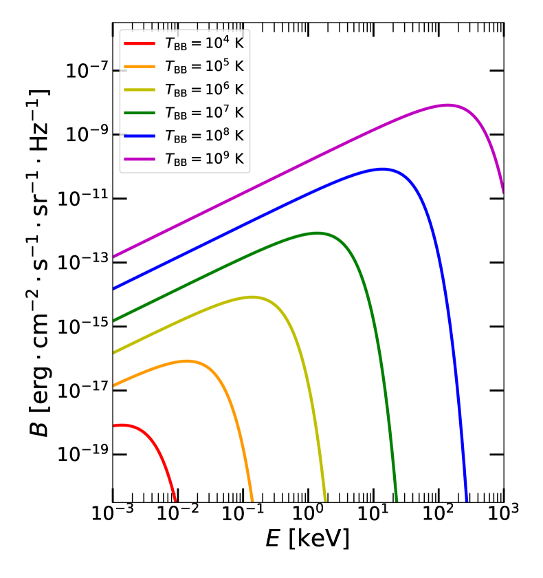
Figure 1.3: The Planck’s law of radiation (1.11) in X-rays.

Numerical codes often require efficient transcription for physical elements that change the polarisation state of a macroscopic electromagnetic signal traveling otherwise in vacuum. If the Stokes parameters are held in 4-dimensional Stokes vector $\vec{S}=(I,Q,U,V)$, then any suitable matrix transformation can represent the change of the polarisation state along the light trajectory. This is referred to as “Müller formalism” with “Müller matrices” (Müller, 1948). This representation is equivalent to the “Jones formalism”, which operates with the $x$- and $y$-amplitudes and phases of the electric field in complex exponential notation that are put into a vector and any series of optically active elements changing polarisation are similarly the “Jones matrices” (Jones, 1941).

1.1.2 X-ray polarigenesis

Number of processes occurring in nature that alter the polarisation state have been observed and theoretically understood. They all involve internal asymmetry of the optically active element with respect to radiation. In astrophysical situations, these are typically scatterings (Thomson scattering, Compton scattering, Rayleigh scattering, resonant scattering, Raman scattering, or Mie scattering on dust grains), which cause linear polarisation along a well-defined direction on spherical particles or on collectively oriented grains with elongated shapes in optically thick media, e.g. dust clouds in interstellar medium (ISM) (Chandrasekhar, 1960; Serkowski et al., 1975; Born et al., 1999; Draine, 2003; Trippe, 2014). Then the linear or circular dichroic media, such as environments with long-chain molecules, helically shaped molecules or plasma in the presence of magnetic field, may cause that one component of the wave in the transverse plane experiences stronger attenuation while passing through (Angel, 1974; Wolstencroft, 1974; Huard, 1997; Born et al., 1999). The synchrotron radiation emits elliptically polarized light due to geometric projections of relativistically gyrating electric charges around magnetic field lines (Ginzburg and Syrovatskii, 1965; Rybicki and Lightman, 1979). The radio observations of ISM often reveal the Zeeman effect on spectral lines in the presence of magnetic field (and the anomalous Zeeman effect, and the Goldreich-Kylafis effect for unresolved cases) that causes the resulting split spectral lines to be either linearly or circularly polarized, depending on the viewing angle towards the magnetic field lines (Zeeman, 1897; Preston, 1898, 1899; Goldreich and Kylafis, 1981, 1982; Elitzur, 2002). The Hanle effect in fluorescent gases permeated by weak magnetic field results in linear polarisation genesis (Hanle, 1924; Stenflo, 1982). Linear polarisation emerges also due to reflections on refractive boundary between two homogeneous media and linear or circular polarisation arises in birefringence crystals and similarly in ISM plasma with external static homogeneous magnetic field, i.e. the Faraday rotation effect (Chandrasekhar and Fermi, 1953; Burn, 1966; Pacholczyk and Swihart, 1970; Rybicki and Lightman, 1979; Fowles, 1989; Tribble, 1991; Huard, 1997; Born et al., 1999). In high-energy astrophysics and QFT, we also encounter possible testing of axion-like particles through X-ray polarimetry and the quantum electrodynamic effect of vacuum birefringence (Heisenberg and Euler, 1936; Heyl and Shaviv, 2000; Pavlov and Zavlin, 2000; Heyl and Shaviv, 2002; Toma et al., 2012; Day and Krippendorf, 2018; Caiazzo et al., 2022). And as it was already mentioned, GR effects alter polarisation of light in vacuum too (Connors and Stark, 1977; Connors et al., 1980).

We refer to Trippe (2014) for a recent review on astrophysical polarisation and further literature on the above. Here, we will elaborate slightly more on those processes that are important in the X-rays near black holes. Because unpolarized emission depolarizes (by dilution) any partially polarized beam of different origin, we will also briefly describe those elementary processes that produce unpolarized emission and are assumed to be important in the studied environments. Many discussed numerical codes implement some forms of absorption, which is also important for the net emerging polarisation state, if fraction of (un)polarized radiation is taken away in particular direction.

Up to our knowledge at scales considered, no microscopic interactions are directly coupled with gravity effects that alter the entire space and time background through curvature, i.e. the curvature field is separable and depends only on the net energy and momentum tensor. Thus, we will describe the GR effects on polarisation inside the follow-up section that provides the equations of radiative transfer, the global GR setup of this work and our additional “linearized” simplification (a given vacuum Kerr background, no self-gravitating elements typical for non-linear general-relativistic magneto-hydro-dynamical simulations) that will allow us to embed all in a simple separable relativistic radiative transfer treatment.

We will omit the discussion of Faraday rotation and vacuum birefringence, as it will not be solved for magnetic fields in this dissertation, but we refer to e.g. Caiazzo and Heyl (2018); Krawczynski et al. (2021) for estimations of possible effects in X-rays.

Thermal emission

All matter with non-zero temperature emits thermal radiation, because any movements of particles in the material causes charge acceleration or dipole oscillation, which produces electromagnetic radiation. If the object approximates a black body (e.g. an optically thick accretion disc with sharp density drop in the photosphere) and thermal equilibrium is reached, the emission intensity profile per unit frequency is isotropic and according to Planck’s law (Planck, 1901; Rybicki and Lightman, 1979):

$$B=\frac{2h_{\textrm{P}}\nu^{3}}{c^{2}}\frac{1}{e^{\frac{h_{\textrm{p}}\nu}{k_{\textrm{B}}T_{\textrm{BB}}}}-1}\textrm{ ,}$$ (1.11)

where $T_{\textrm{BB}}$ is the body’s temperature and $k_{\textrm{B}}=1.381\times 10^{-16}\,\textrm{erg}\cdot\textrm{K}^{-1}$ is the Boltzman’s constant.

In the treatment of disc photospheres, we will sometimes use the effective temperature $T_{\textrm{eff}}=T_{\textrm{BB}}$ that characterizes radiation field of a quasi-thermal medium, i.e. it assigns the effective temperature value, as if it was a black body. For simplicity, the radiative transfer codes often assume a local thermodynamic equilibrium (LTE), characterized by optically thick environment (photon’s mean free path is shorter than characteristic length) and $I=B$, thus we also assume some mean local temperature. For the black-body emission to peak in the X-ray band, it requires extreme temperatures of $T_{\textrm{BB}}\gtrapprox 10^{5}$ K (see Figure 1.3). Black-body radiation is always unpolarized, as there is no internal asymmetry in the thermal pool.

Scattering on particles

Thermal emission can, however, gain some polarisation through scattering on electrons (bound or free, although for X-rays above 1 keV the distinction does not matter for gas mostly composed of hydrogen, Vainshtein et al., 1998) or dust grains. In the X-rays, we are mostly interested in Compton scattering of photons on free electrons, which is called Thomson scattering in the inelastic limit – applicable when $h_{\textrm{P}}\nu$ of the incoming photon becomes comparable to the electron rest energy $m_{\textrm{e}}c^{2}$.

Let us list the formulae for unpolarized incident photon, which can be found in e.g. McMaster (1961); Fernández et al. (1993); Matt et al. (1996c) more generalized. The photon’s energy changes after the interaction as (Compton, 1923)

$$\varepsilon^{\prime}=\dfrac{\varepsilon}{1+\dfrac{\varepsilon}{m_{e}c^{2}}(1-\cos\Theta)}\textrm{ ,}$$ (1.12)

where $\varepsilon$ and $\varepsilon^{\prime}$ are photon energies before and after the scattering at an angle $\Theta$, respectively. The cross-section $\sigma_{\textrm{KN}}$ of Compton scattering is expressed by the Klein-Nishina formula (Klein and Nishina, 1929)

$$\sigma_{\textrm{KN}}=\dfrac{3}{4}\sigma_{\textrm{T}}\Big{\{}\dfrac{1+u}{u^{3}}\Big{[}\dfrac{2u(1+u)}{1+2u}-\log(1+2u)\Big{]}+\dfrac{\log(1+2u)}{2u}-\dfrac{1+3u}{(1+2u)^{2}}\Big{\}}\textrm{ ,}$$ (1.13)

where $u=h_{\textrm{P}}\nu/m_{\textrm{e}}c^{2}$ and $\sigma_{\textrm{T}}=8\pi e_{\textrm{C}}^{4}/3m_{\textrm{e}}^{2}c^{4}$ is the classical Thomson cross section, where $e_{\textrm{C}}$ is the elementary charge. The differential cross section for electrons at rest is (e.g. Matt et al., 1996c)

$$\frac{\textrm{d}\sigma_{\textrm{KN}}}{\textrm{d}\omega}=\dfrac{1}{2}\frac{e_{\textrm{C}}^{2}}{m_{\textrm{e}}c^{2}}\left(\frac{\varepsilon^{\prime}}{\varepsilon}\right)^{2}\left[\left(\frac{\varepsilon^{\prime}}{\varepsilon}\right)+\left(\frac{\varepsilon}{\varepsilon^{\prime}}\right)-\sin^{2}\Theta\right]\textrm{ .}$$ (1.14)

Figure 1.5 illustrates how the passing photon can gain linear polarisation, which is applicable also to other types of scatterings. The resulting polarisation is perpendicular to the “scattering plane” given by the incident and emission directions.

The resulting degree of polarisation for Compton scattering is given more pricesely for unpolarized incident photons by (Hudson, 1968)

$$p_{\textrm{C}}=\dfrac{\sin^{2}\Theta}{\dfrac{\varepsilon}{\varepsilon^{\prime}}+\dfrac{\varepsilon^{\prime}}{\varepsilon}-\sin^{2}\Theta}\textrm{ .}$$ (1.15)

Thus it depends on energy and, for an initially unpolarized beam, the polarisation of $p=100\%$ is never achieved. The degree of polarisation as a function of the scattering angle $\Theta$ is shown in Figure 1.5 for different initial photon energies. In simulations we then typically utilize these relations, combined with their generalization for polarized incident photons, and then for the fraction of polarized photons $p$ the polarisation vector $\vec{P}$ (a unit vector parallel to $\vec{E}$) of the scattered photon is (Angel et al., 1969)

$$\vec{P}=\frac{(\vec{P}_{0}\times\vec{e}_{\textrm{z}})\times\vec{e}_{\textrm{z}}}{|\vec{P}|}\textrm{ ,}$$ (1.16)

where $\vec{P}_{0}$ is the incident polarisation vector and $\vec{e}_{\textrm{z}}$ is the unit vector in the scattered direction. The remaining fraction $1-p$ has the polarisation vector randomly distributed in the polarisation plane. Multiple scatterings often result in net depolarisation of the emergent radiation, because each scattering event occurs in generally different direction with different photon energy change.

Figure 1.4: Explanation of linear polarisation induced by scattering in particular geometry. Gray plane is called the plane of scattering. Image from Trippe (2014).

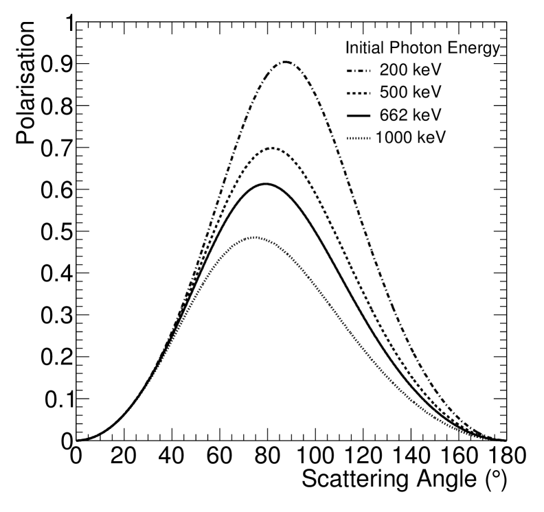
Figure 1.5: Degree of linear polarisation $p_{\textrm{C}}$ induced by Compton scattering as a function of scattering angle $\Theta$ for a few cases of initial photon energy $\varepsilon$. Image from Knights et al. (2018).

In the limit of low initial energies (i.e. the Thomson scattering), the curve shown in Figure 1.5 becomes symmetric around $\Theta=90^{\circ}$, can reach $p=100\%$, and follows a simple law:

$$p_{\textrm{T}}=\dfrac{1-\cos^{2}\Theta}{1+\cos^{2}\Theta}\textrm{ .}$$ (1.17)

When the incident photon possesses higher energy than the electrons, we refer to “Compton down-scattering” and the photon looses energy after it scatters. In extremely hot plasma in the vicinity of black holes, the situation can be reversed and photons can gain energy from ultra-relativistic electrons (with mean speeds comparable to $c$). Then we refer to “Compton up-scattering”, “inverse Compton scattering”, or “Comptonization” for the case of multiple scatterings. A proper quantum treatment is required to fully describe this effect, but in the case of up-scattered thermal emission, it typically collectively leads to moderately polarized power-law emission in the case of coronae near accretion discs (Rybicki and Lightman, 1979; Sunyaev and Titarchuk, 1980, 1985). We refer to Bonometto et al. (1970); Nagirner and Poutanen (1993); Poutanen and Vilhu (1993); Poutanen and Vurm (2010) for the analytical treatment of polarisation due to Compton up-scattering. For a relativistic isotropic electron gas, the resulting polarisation is zero (Bonometto et al., 1970).

Synchrotron emission

Black-hole accreting systems often possess extreme magnetic fields ($\approx 10^{4}$ G for supermassive black holes, $\approx 10^{8}$ G for stellar-mass black holes, measured as accretion disc magnetic strength, see Daly, 2019). Polarized synchrotron emission is particularly known to be a magnetic field structure tracer near the black-hole horizon in the radio band (Event Horizon Telescope Collaboration, 2021). But the resulting polarized synchrotron emission, sometimes referred to as “magneto-bremsstrahlung”, of electrons gyrating around magnetic field lines can affect the net output even in the X-rays (Ginzburg and Syrovatskii, 1965; Weisskopf et al., 2022). The emergent polarisation is orthogonal to the magnetic field and the details of polarisation computation, including absorption, can be found in e.g. Leung et al. (2011).

The disordering of magnetic field by turbulences and shocks, and multiple scatterings can wash out the primary polarisation gain. For astrophysically realistic plasmas with a partially disordered magnetic field and $0<\bar{\alpha}<1$, where $\bar{\alpha}$ sets the power in the usually assumed power-law distribution of electron energies, the degree of linear polarisation is not expected to exceed $p\approx 16\%$ (Pacholczyk, 1970). For circular polarisation the realistic estimates are $p_{\textrm{c}}\lessapprox 1\%$ (Angel, 1974).

In X-rays, we often encounter synchrotron self-Compton radiation, which are photons that get inverse Compton scattered by the same electrons that caused synchrotron emission due to acceleration in magnetic field (see e.g. Ghisellini, 2013). Unpolarized synchrotron photons result in synchrotron self-Compton emission with small ($<5$%) polarisation fraction for all but very low Lorentz factors describing the mean particle speeds with respect to $c$ (Begelman and Sikora, 1987; Celotti and Matt, 1994).

Bremsstrahlung

At soft X-rays, we typically encounter one other form of free-free radiation. This is the free-free absorption or emission of photons when free electron accelerates in the electric field of positively charged atomic nucleus (Rybicki and Lightman, 1979). This effect is often called “thermal bremsstrahlung”, although it is not truly thermal, in comparison to black-body emission.

The cross-section exponentially decays towards high energies, and the effects are expected to be non-negligible in the X-ray band for hot gases with electron temperatures $T_{\textrm{e}}\gtrapprox 10^{6}\textrm{ K}$ (Seward and Charles, 2010). It may impact the net polarisation emerging nearby accreting black holes by means of absorption, and perhaps more importantly by means of emission, because the cross-section for bremsstrahlung is polarisation dependent (Gluckstern and Hull, 1953). For the mid (1–10 keV) and hard ($>10$ keV) X-rays, for example Haug (1972); Komarov et al. (2016); Krawczynski et al. (2023) provide calculations of polarized bremsstrahlung emission for pressure anisotropy of electrons in solar flares, galaxy clusters and black-hole accretion discs, respectively. In the last case it is shown that in combination with Comptonization it may lead to surprisingly high (tens of %) linear polarisation fraction.

Photoelectric effect

An important class of processes in the X-rays is the photoionization of electrons and recombination, i.e. the bound-free absorption and emission. The cross-section for photoelectric absorption is affected by particular ionization edges, but in the X-rays generally declines as $\sim E^{-3}$ (see e.g. García et al., 2013). The condition of hydrostatic equilibrium for e.g. accretion disc’s plane-parallel atmosphere, can be replaced by even simpler assumption of constant pressure or constant density. In the latter case, a very useful quantity called ionization parameter $\xi$ $[\textrm{erg}\cdot\textrm{cm}\cdot\textrm{s}^{-1}]$ can be defined as (Tarter et al., 1969)

$$\xi=\dfrac{4\pi\int_{0}^{\infty}F_{\textrm{E}}\textrm{d}E}{n_{\textrm{H}}}\textrm{ ,}$$ (1.18)

where $n_{\textrm{H}}$ is the neutral hydrogen density in the medium, $F_{\textrm{E}}$ is the radiation flux received at one location on the disc surface. It represents the competition between the photoionization rate ($\sim n_{\textrm{H}}$) and recombination rate ($\sim n_{\textrm{H}}^{2}$) inside the irradiated medium. Although recombination produces unpolarized photons, the photoelectric cross-section is dependent on the incident polarisation state, which is utilized in the gas-pixel detectors on board of IXPE (see Section 1.2.1).

Spectral lines

The surroundings of accreting supermassive and stellar-mass black holes produce many emission and absoprtion lines in the X-rays caused by bound-bound electron transitions inside atoms. Absorption lines typically emerge from cold gas irradiated by hotter thermalized medium behind from observer’s point of view. Emission lines are typically a result of reflection. Fluorescent lines are unpolarized, but resonant line scattering may cause non-negligible polarisation (Lee, 1994; Lee et al., 1994; Lee and Blandford, 1997), depending on the competing Auger effect. The polarisation of the scattered line emission depends on the quantum numbers characterizing the electronic transition in each resonant line. It results in a wide range in strength, but may become as relevant as for Thomson scattering.

Due to the “iron peak” in nuclear binding energy curve of chemical elements, iron is quite omnipresent in the universe, including nearby supermassive and stellar-mass black holes. Therefore, in the X-rays, we typically encounter a photoelectric absorption by inner shells of partially ionized iron atoms, which results into excited state and immediate decay. This is done through either Auger de-excitation (e.g. with $66\%$ probability for $n=1$ shell of the iron atom, Fabian et al., 2000) or characteristic fluorescent line X-ray emission, where the emitted photon may escape to the observer or encounter further interactions. The details of bound-bound processes require quantum treatment and are highly dependent on local physical conditions, similarly to ionization.

All spectral lines originate at single energy values, but are broadened by vast number of physical effects. It is out of the scope of this dissertation to provide the theoretical background, but from non-relativistic effects we name the Doppler broadening due to thermal velocities, turbulences and large-scale velocities, natural broadening and pressure broadening. The relativistic line broadening will be discussed in the next section. We refer to e.g. Castor (2004) for more details on the emergence and properties of spectral lines or ionization and recombination.

1.1.3 Combined radiative transfer

We briefly provide below the theoretical framework for numerical solving of radiative processes that is used in this work. In addition to these, we examine Monte Carlo (MC) methods (see e.g. Cashwell and Everett, 1959) that rely on injecting photons in the configuration space, ray tracing and calculating probabilities for absorption and scattering.

Radiative transfer in astrophysical materials in local frame of reference

When numerically solving for a radiation solution in interaction with partially ionized medium in plane-parallel static approximation, we typically discretize the medium in vertical layers, provide boundary conditions and iterate for temperature, pressure and fractional abundance of atomic species inside the medium the one-dimensional equation of radiative transfer (Chandrasekhar, 1960):

$$\mu_{\textrm{e}}\dfrac{\textrm{d}I}{\textrm{d}\tau}=I-\tilde{S}\,,$$ (1.19)

where $\mu_{\textrm{e}}$ is cosine of the inclination angle from the slab’s normal and $\tilde{S}$ is the frequency dependent source function that combines all absorption, emission and scattering processes contributions in an infinitely wide slab parametrized in the remaining dimension by optical depth $\tau$, again frequency dependent and proportional to geometrical depth $l$ measured from the side of the slab (in all cases for disc atmospheres, we will assume this side to be a fictitious disc surface, below which the $\tau$ reaches infinity in optically thick regime). In non-LTE conditions, we have to solve the equation of statistical equilibrium (Castor, 2004)

$$n_{i}\sum_{j\neq i}P_{ij}-\sum_{j\neq i}n_{j}P_{ji}=0\,,$$ (1.20)

where $P_{ij}$ are all ionization and excitation rates for both radiative and collisional processes, $P_{ji}$ are all recombination and de-excitation rates and $n_{x}$ are the corresponding number densities for the species that we account for. Polarized radiative calculus in materials is well developed (e.g. Chandrasekhar, 1960; Sobolev, 1963; Stenflo, 1994; Landi Degl’Innocenti and Landolfi, 2004), but will not be used in this work, therefore we omit the theoretical background.

General-relativistic radiative transfer in vacuum

We consider a single rotating black hole in this work and the rest of the universe is simply non-gravitating. Although this is a notable simplification and many times the axial and equatorial symmetry allows significant reductions in calculation of light trajectories and polarisation, analytical operations within the Kerr metric typically require extensive acrobatics with trigonometric functions. This is clear already from the derivation of the solution and e.g. Chandrasekhar writes on perturbation studies of the Kerr metric (Chandrasekhar, 1983): “… the analysis has led us into a realm of the rococo: splendorous, joyful, and immensely ornate.”

Despite challenging details, a Kerr black hole can be fully described only by mass $M$ and angular momentum $J$. We do not consider electric charge, because it is widely believed that in astrophysical black holes any excess of electric charge would autoneutralize, although this is still a matter of debate with the latest EHT results (Kocherlakota et al., 2021; Event Horizon Telescope Collaboration, 2022).

One of the simplest representations of the Kerr metric components from the length element $\textrm{d}s$ is in Boyer-Lindquist coordinates ($t$,$r$,$\theta$,$\phi$) (Boyer and Lindquist, 1967), being a natural generalization of the Schwarzschild coordinates: (e.g. Visser, 2007)

$$\begin{split}\textrm{d}s^{2}=g_{\mu\nu}\textrm{d}x^{\mu}\textrm{d}x^{\nu}&=-\left(1-\frac{2Mr}{r^{2}+a^{2}\cos^{2}{\theta}}\right)\textrm{d}t^{2}-\frac{4Mra\sin^{2}{\theta}}{r^{2}+a^{2}\cos^{2}{\theta}}\textrm{d}t\textrm{d}\phi\\ &\quad+\left(\frac{r^{2}+a^{2}\cos^{2}{\theta}}{r^{2}-2Mr+a^{2}}\right)\textrm{d}r^{2}+(r^{2}+a^{2}\cos^{2}{\theta})\textrm{d}\theta^{2}\\ &\quad+\left(r^{2}+a^{2}+\frac{2Mra^{2}\sin^{2}{\theta}}{r^{2}+a^{2}\cos^{2}{\theta}}\right)\sin^{2}{\theta}\textrm{d}\phi^{2}\,,\end{split}$$ (1.21)

where we used the specific angular momentum $a=J/M$, the “black-hole spin”, which has a reduced range of $-1\leq a\leq 1$ and is considered in this work only in one, positive direction of rotation, given by angular 3-velocity $\vec{\Omega}$. In fact, Thorne (1974) calculated a maximal theoretical rotation value to be $a=0.998$ for a standard accretion disc (see below).

We assume the surrounding disc to be corotating with the black hole and residing geometrically thin in the equatorial plane ($\theta=\pi/2$), but we note that this is another simplification that is in fact hard to justify. We note that there are many works studying misaligned rotation, counter rotation, or self-gravitating discs and other departures from the Kerr metric (e.g. Bardeen and Petterson, 1975; Laor and Netzer, 1989; Collin and Zahn, 1999; Karas et al., 2004; Collin and Zahn, 2008; Nixon et al., 2012; Nixon, 2012; Krawczynski, 2012, 2018; Tripathi et al., 2020; Hrubeš, 2022). Our estimates should thus serve as first-order approach.

If $a=0$, the solution (1.21) becomes a Schwarzschild solution and the inner-most circular orbit (ISCO) is located at 6 gravitational radii ($6\,r_{\textrm{g}}=6\,GM/c^{2}$ in non-geometrical units). If $a=1$, the ISCO is much closer to the black-hole: at $1\,r_{\textrm{g}}$. This is important for the allowed accretion disc’s inner extension (see below). In this study, we will not consider any light escaping from the infalling matter below ISCO, which is as well a debatable simplification (e.g. Dovčiak et al., 2004a). The region between the (outer) event horizon and between the Killing horizon (where Killing vectors are null, Carroll, 2004), is called the “ergosphere” and is important for explanation of the work necessary on observed ejected material in polar directions through the Penrose process (Penrose, 1969). For a full theoretical background we refer to e.g. Misner et al. (1973).

The polarized radiative transfer calculations used in this dissertation are departing from the fundamental works of Cunningham and Bardeen (1973); Cunningham (1975); Connors and Stark (1977); Connors et al. (1980), which we summarize here below. Photon trajectories follow the geodesic equation

$$\dfrac{dp^{\mu}}{d\lambda^{\prime}}+\Gamma_{\sigma\tau}^{\mu}p^{\sigma}p^{\tau}=0\textrm{ ,}$$ (1.22)

where $p^{\mu}=\frac{dx^{\mu}}{d\lambda^{\prime}}$ is a four-momentum of light, $\lambda^{\prime}$ is affine parameter of a geodesic, and $\Gamma_{\mu\nu}^{\sigma}$ are Christoffel symbols for the Kerr metric. Brandon Carter (*1942) derived constants of motion that fully describe any test particle motion outside of the Kerr black hole (Carter, 1968). The lensing effects are captured by the equation of geodesic deviation

$$\dfrac{d^{2}Y_{j}^{\mu}}{d\lambda^{\prime 2}}+2\Gamma_{\sigma\gamma}^{\mu}p^{\sigma}\dfrac{dY_{j}^{\gamma}}{d\lambda^{\prime}}+\Gamma_{\sigma\tau,\gamma}^{\mu}p^{\sigma}p^{\tau}Y_{j}^{\gamma}=0\textrm{ , }j=1,2\textrm{ ,}$$ (1.23)

where $Y_{j}^{\mu}$ are two vectors characterizing the distance between nearby geodesics. These equations are to be numerically integrated over the journey of a photon, in order to obtain a distorted picture that the observer will obtain, since the trajectories and energies of photons deviate from the classical Newtonian framework. All SR and GR effects are then automatically included, namely the kinetic and gravitational frequency shifts, relativistic aberration, the emission direction changes, gravitational lensing and bending effects and relative time delays. The relativistic effects on broadening of spectral lines are illustrated in Figure 1.7 for ratios of observed and emitted radiation frequencies $\nu_{\textrm{obs}}$ and $\nu_{\textrm{em}}$, respectively. It serves as a tool for black-hole spin spectral fitting from X-ray radiation reflected from accretion disc, typically performed on the strong iron line complex at 6–7 keV, alongside spectral fits of the underlying continuum that also varies with black-hole spin.

To obtain $F_{\textrm{E}}^{\Omega_{0}}$ at a distant detector that sees, as a point-source, an emitting accretion disc at inclination angle $\theta$ (coinciding with the Boyer-Lindquist coordinate $\theta$), measured from the rotational axis of the disc, with local intensity $I$, we integrate

$$F_{\textrm{E}}^{\Omega_{0}}=\int_{r_{\textrm{in}}}^{r_{\textrm{out}}}\int_{g_{\textrm{min}}}^{g_{\textrm{max}}}g^{3}If\textrm{ d}g\textrm{d}r$$ (1.24)

over the area of the disc with radial coordinate $r$ extending from $r_{\textrm{in}}$ in the outer vicinity of the black-hole horizon to arbitrary $r_{\textrm{out}}$. We only aim to cover one side of the disc and possible photons arriving from the far side of the disc due to non-zero curvature are neglected. And in most of the results, we also neglect reflections of photons that escape the disc and due to strong gravity arrive back to the disc (the returning radiation), i.e. neither to the event horizon, neither to the spatial infinity. Keplerian disc rotation is assumed, which is not needed for the local emission itself, but the assumed velocities $U^{(\phi)}\sim r^{-3/2}$ affect the shifts upon locally emitted radiation. In (1.24), $f$ is the transfer function that represents the Jacobian of the transformation from the detector’s viewing position – typically calculated in impact coordinates (Cunningham and Bardeen, 1973) $\alpha$ and $\beta$ measured perpendicular to and parallel with the spin axis of the black hole projected onto the observer’s sky, respectively – towards the disc area in the integration coordinates, here $g$ (see below) and $r$. The transfer function then includes all of the effects above upon the photon’s journey and acts as an amplifier or damper of different disc sections. We define $n_{\textrm{em}}$ as the local emission angle measured from the principal system axis and $g=E_{\textrm{obs}}/E_{\textrm{em}}$ as the energy shift from the emitted photon energy $E_{\textrm{em}}$ to the observed one $E_{\textrm{obs}}$. The energy shift is directly related to the Boyer-Lindquist coordinate $\phi$, being the azimuthal coordinate over the disc. Therefore, $g$ may also be used as a distinct azimuthal coordinate. Both of these have their minima and maxima, $g_{\textrm{min}}$, $\phi_{\textrm{min}}$ and $g_{\textrm{max}}$, $\phi_{\textrm{max}}$ respectively, for $g$ depending on the emission radius studied.

Equation (1.24) may be rewritten in terms of observed photon flux $N_{\textrm{E}}^{\Omega_{0}}$ in an equally useful way (see e.g. Dovčiak, 2004):

$$N_{\textrm{E}}^{\Omega_{0}}=N_{0}\int_{r_{\textrm{in}}}^{r_{\textrm{out}}}\int_{\phi_{\textrm{min}}}^{\phi_{\textrm{max}}}I_{\textrm{N}}g\cos(n_{\textrm{em}})\bar{l}r\textrm{ }\textrm{d}\phi\textrm{d}r\textrm{ ,}$$ (1.25)

where $N_{0}$ is the normalization constant, $I_{\textrm{N}}=I/h_{\textrm{P}}\nu_{\textrm{em}}$ is the local photon intensity at $\nu_{\textrm{em}}$, $\bar{l}$ is the so-called lensing factor for far-away sources obtained from (1.23), and the combination of parameters $g^{2}\cos(n_{\textrm{em}})\bar{l}$ is an analogue of the transfer function $f$ from the former case. The transformation from local disc coordinates to the image that a distant observer would see is illustrated in Figure 1.7. The energy shift of a photon for an example of $a=1$ and $\theta=85^{\circ}$ in the equatorial $x=\sqrt{r^{2}+a^{2}}\cos{\phi}$ and $y=\sqrt{r^{2}+a^{2}}\sin{\phi}$ Cartesian coordinates and the impact parameters $\alpha$ and $\beta$ on the plane of the sky is shown in Figure 1.8. For other examples and maps of the GR emission vector change, or the transfer function itself, see Dovčiak (2004).

Figure 1.6: Illustration of the spectral line broadening due to classical Dopler shift, SR Doppler effect and aberration, GR energy shift and the net effect (from top to bottom). Image from Fabian et al. (2000).

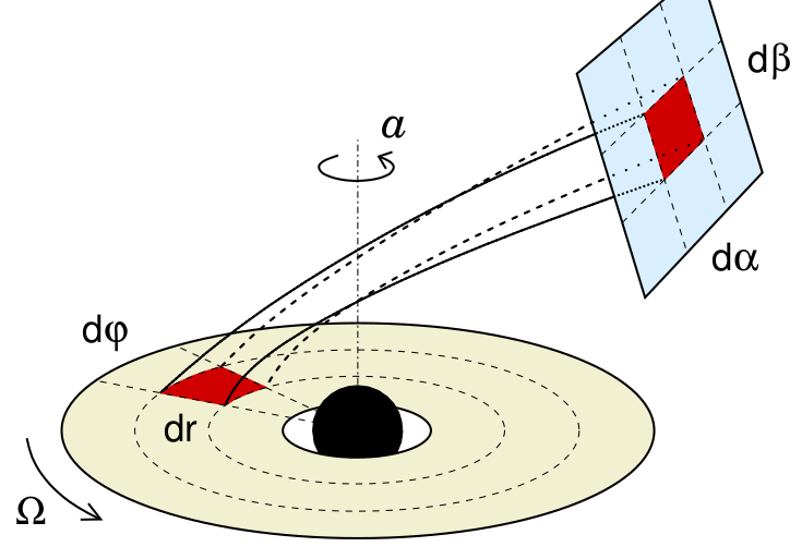
Figure 1.7: Illustration of the transformation from local frame of reference, comoving with the accretion disc to the image on the sky. We define the disc area element typically in the Boyer-Lindquist coordinates $r$ and $\phi$ and the projected area that the observer sees in the impact parameters $\alpha$ and $\beta$. Image courtesy of Michal Dovčiak.

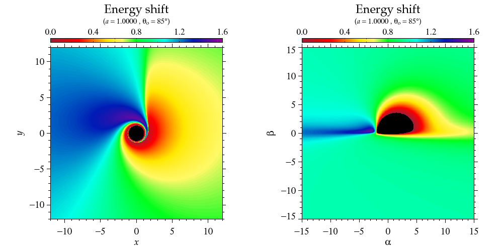
Figure 1.8: The energy shift, $g$, in Kerr spacetime for the case of $a=1$ and $\theta=85^{\circ}$ in the equatorial $x$ and $y$ coordinates (left) and the impact parameters $\alpha$ and $\beta$ (right). Image courtesy of Michal Dovčiak.

The previous paragraph developed for Stokes $I$ is equally valid for other Stokes parameters. It is, however, the polarisation angle that continuously rotates along a geodesic climbing up the potential well, which is apparent from parallel transport of the polarisation vector, residing in the polarisation plane perpendicular to the photon momentum. Then, for a distant observer, the total polarisation degree is also altered, if GR effects are included. We typically expect relativistic depolarisation on the total signal, because individual light rays are affected differently, although that is not always the case and in rare cases the polarisation can be amplified (Dovčiak et al., 2011). We provide the integration formulae for all Stokes parameters at once

$$\begin{split}\Delta I_{\textrm{obs}}(E_{\textrm{obs}},\Delta E_{\textrm{obs}})&=N_{0}\iint Ir\cos(n_{\textrm{em}})g^{2}\bar{l}\textrm{ }\textrm{d}S\textrm{ ,}\\ \Delta Q_{\textrm{obs}}(E_{\textrm{obs}},\Delta E_{\textrm{obs}})&=N_{0}\iint[Q\cos(2\Delta\Psi)\\ &\quad-U\sin(2\Delta\Psi)]r\cos(n_{\textrm{em}})g^{2}\bar{l}\textrm{ }\textrm{d}S\textrm{ ,}\\ \Delta U_{\textrm{obs}}(E_{\textrm{obs}},\Delta E_{\textrm{obs}})&=N_{0}\iint[Q\sin(2\Delta\Psi)\\ &\quad+U\cos(2\Delta\Psi)]r\cos(n_{\textrm{em}})g^{2}\bar{l}\textrm{ }\textrm{d}S\textrm{ ,}\\ \Delta V_{\textrm{obs}}(E_{\textrm{obs}},\Delta E_{\textrm{obs}})&=N_{0}\iint Vr\cos(n_{\textrm{em}})g^{2}\bar{l}\textrm{ }\textrm{d}S\textrm{ .}\end{split}$$ (1.26)

where $\textrm{d}S$ denotes the planar integration across the disc in any coordinates and $\Delta\Psi$ is the total change of the linear polarisation angle between the emission point (here at the disc) and the receiving point (here at the detector located at spatial infinity). In numerical codes that we will operate with, it is useful to also integrate the resulting photon flux $N_{\textrm{E}}^{\Omega_{0}}$ and analogic quantities for $Q$, $U$, $V$ over the final energy bin with size $\Delta E_{\textrm{obs}}$ at $E_{\textrm{obs}}$, in order to obtain the Stokes parameters $\Delta I_{\textrm{obs}}(E_{\textrm{obs}},\Delta E_{\textrm{obs}})$, $\Delta Q_{\textrm{obs}}(E_{\textrm{obs}},\Delta E_{\textrm{obs}})$, $\Delta U_{\textrm{obs}}(E_{\textrm{obs}},\Delta E_{\textrm{obs}})$, $\Delta V_{\textrm{obs}}(E_{\textrm{obs}},\Delta E_{\textrm{obs}})$ in the units of $[\textrm{counts}\cdot\textrm{sr}^{-1}\cdot\textrm{s}^{-1}]$, which set the number of photons measured per energy bin (and inside the code we would set a distance to obtain results per detector unit area). Again, we will assume $\Delta V_{\textrm{obs}}=0$ in this work. We will often drop the “obs” and “em” subscripts when obvious from the context.

The acquisition of $\Delta\Psi$ between two spatial points is analytically possible in many cases, unlike the solutions to the geodesic equation and equation of geodetic deviation that are typically numerically integrated. This is because of the Walker-Penrose theorem (Walker and Penrose, 1970) that is derived in the Newman-Penrose formalism of GR (Newman and Penrose, 1962, 1963), invoking complex calculus. A complex constant of motion $\kappa=\kappa_{2}-i\kappa_{1}$, the Walker-Penrose constant, can be expressed for the Kerr metric in Boyer-Lindquist coordinates:

$$\begin{split}\kappa=\frac{1}{r+ia\cos{\theta}}&\{(r^{2}+a^{2})(p_{r}f_{t}-p_{t}f_{r})+a(p_{r}f_{\varphi}-p_{\varphi}f_{r})\\ &\quad+\frac{i}{\sin{\theta}}[p_{\theta}f_{\varphi}-p_{\varphi}f_{\theta}-a\sin^{2}{\!\theta}\,(p_{t}f_{\theta}-p_{\theta}f_{t})]\}\,,\end{split}$$ (1.27)

where $f^{\mu}$ is the polarisation 4-vector parallelly transported along a null geodesic. Hence, in order to find the polarisation angle change, i.e. to find three components of the polarisation 4-vector $f^{\mu}$ in the local reference frame, these three unknown components can be expressed at the receiving point by means of the $\kappa_{1}$ and $\kappa_{2}$ quantities, while $\kappa_{1}$ and $\kappa_{2}$ can be expressed by means of the initial $p^{\mu}$ and $f_{0}^{\mu}$ of each photon at the emission point due to the conservation of $\kappa$. As last step, we construct the local polarisation angle $\Psi$ according to its definition at the receiving point and transform to this frame of reference. The GR effects on polarisation near black holes have been studied extensively since the pioneering 1970s and 1980s research, and the dependency of this effect on inclination, black-hole spin and other fundamental parameters enables independent fitting method via X-ray spectropolarimetry (e.g. Laor et al., 1990; Matt, 1993; Agol and Krolik, 2000; Dovčiak et al., 2004a, 2008; Schnittman and Krolik, 2009, 2010).

1.2 Astronomical X-ray polarimetry

Before we introduce the astrophysical objects of study and estimate the efficiency of X-ray polarisation diagnostics, let us devote a few words to the current status of X-ray polarimetry in astronomy. The information provided in this section is selected from Fabiani and Muleri (2014); Kislat et al. (2015); Di Lalla (2019); Weisskopf et al. (2022); Muleri (2022), to which we also refer for further details.

1.2.1 Detectors

In the literature, we find three classes of astronomical X-ray polarimeters: Bragg diffraction-based polarimeters, scattering-based polarimeters, and polarimeters on the basis of the photoelectric effect. The last category includes gas pixel detectors (GPD) and time projection chambers (TPC) that are most frequently used in contemporary research. The IXPE mission contains a GPD that traces a photo-excited electron path in a gas chamber. The direction of emission of the photoelectron is dependent on the differential cross-section of the interaction, which is correlated to the absorbed photon’s electric vector direction. The projected path of the electron in the sensitive volume is then analyzed using sophisticated methods to provide information on the initial linear polarisation state of each photon. Here we will provide just the basics of such analysis without technological details.

Any linear polarimeter measures the azimuthal modulation of some physical quantity $\bar{R}(\bar{\phi})$, around some direction of polarisation $\bar{\phi}_{0}$ in the polarisation plane. The response of a polarimeter can be characterized by two generic parameters $C$ and $D$:

$$\bar{R}(\bar{\phi})=C+D\cos^{2}(\bar{\phi}-\bar{\phi}_{0})\textrm{ .}$$ (1.28)

Without systematic effects, unpolarized radiation results in statistically flat histogram of the response curve $\bar{R}(\bar{\phi})$ and $100\%$ polarized signal produces strongly modulated histogram of the response curve with some amplitude $D/2$. Figure 1.9 illustrates the two extreme cases. For real polarimeters $C\neq 0$ and we introduce energy-dependent modulation factor $\mu$:

$$\mu=\left.\dfrac{\bar{R}_{\textrm{max}}-\bar{R}_{\textrm{min}}}{\bar{R}_{\textrm{max}}+\bar{R}_{\textrm{min}}}\right|_{p=100\%}=\left.\dfrac{D}{D+2C}\right|_{p=100\%}\textrm{ ,}$$ (1.29)

where $\bar{R}_{\textrm{max}}$ and $\bar{R}_{\textrm{min}}$ denote the maxima and minima of the response curve $\bar{R}(\bar{\phi})$, respectively. The modulation factor directly corresponds to the sensitivity of a given polarimeter. Ideal polarimeter with complete modulation means that $\mu=1$. For good enough photon statistics, we can obtain polarisation degree from the measured modulation amplitude:

$$p=\dfrac{1}{\mu}\dfrac{\bar{R}_{\textrm{max}}-\bar{R}_{\textrm{min}}}{\bar{R}_{\textrm{max}}+\bar{R}_{\textrm{min}}}\textrm{ .}$$ (1.30)

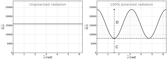
Figure 1.9: Response curves from a fictitious linear polarimeter for fully unpolarized radiation (left) and fully polarized radiation (right). Image adapted from Di Lalla (2019).

In case of low number of photons, which is the usual case for astronomical X-ray polarimetry, the polarisation fraction is, however, best obtained through Stokes parameters in the so-called event-by-event calculation (see Muleri, 2022, for details and comparisons with the approach of fitting the modulation curve). This approach also allows to use weights for photon trajectories in GPDs, which raises the overall sensitivity and reduces statistical errors (Di Marco et al., 2022). We define:

$$i_{k} =1\textrm{ ,}$$ (1.31)

$$q_{k} =\cos(2\bar{\phi}_{k})\textrm{ ,}$$

$$u_{k} =\sin(2\bar{\phi}_{k})\textrm{ ,}$$

for each photon arrival (indexed by $k$) at the instrument-defined direction $\bar{\phi}_{k}$. The linearity of Stokes parameters allows to sum:

$$\tilde{I}_{\textrm{N}} =\dfrac{1}{T_{\textrm{obs}}}\sum_{k=1}^{N}i_{k}\textrm{ ,}$$ (1.32)

$$\tilde{Q}_{\textrm{N}} =\dfrac{1}{T_{\textrm{obs}}}\sum_{k=1}^{N}q_{k}\textrm{ ,}$$

$$\tilde{U}_{\textrm{N}} =\dfrac{1}{T_{\textrm{obs}}}\sum_{k=1}^{N}u_{k}\textrm{ ,}$$

for a measurement in $[\textrm{counts}\cdot\textrm{s}^{-1}]$ of $N$ events per energy band over the exposition time $T_{\textrm{obs}}$ (here the Stokes parameters are not in the units per unit area, which is the reason for the tilde notation). Then Equations (1.28) and (1.30) provide expressions for measured polarisation degree $p$ and polarisation angle $\Psi$

$$p =\dfrac{2}{\mu}\dfrac{\sqrt{\tilde{Q}_{\textrm{N}}^{2}+\tilde{U}_{\textrm{N}}^{2}}}{\tilde{I}_{\textrm{N}}}\textrm{ ,}$$ (1.33)

$$\Psi =\dfrac{1}{2}\textrm{ }\textrm{arctan}_{2}\left(\dfrac{\tilde{U}_{\textrm{N}}}{\tilde{Q}_{\textrm{N}}}\right)\,.$$

One can equivalently define $\mu$-normalized Stokes parameters $Q$ and $U$ to account for the instrumental quality.

Even for unpolarized photons, real polarimeters detect non-zero modulation amplitude due to Poisson-distributed statistical fluctuations. To quantify the maximum polarisation, which can be produced by stochastic noise only (in the absence of true source polarisation), at a certain $X\%$ confidence level, we use the minimum detectable polarisation function $M\!D\!P_{X\%}$. It can be derived that for $99\%$ confidence level and in case of non-negligible background (Elsner et al., 2012):

$$M\!D\!P_{99\%}=\dfrac{4.29}{\mu}\dfrac{\sqrt{N_{\textrm{S}}+N_{\textrm{B}}}}{N_{\textrm{S}}}\textrm{ ,}$$ (1.34)

where $N_{\textrm{S}}$ is the number of events received from the actual source, $N_{\textrm{B}}$ is the number of events from the background contribution to the measurement. Thus, the criterion of observed polarisation with $3\sigma$ statistical uncertainty above zero is not enough for an objectively credible polarisation detection. In addition, the observed polarisation degree value is required to appear above $M\!D\!P_{99\%}$ to claim a statistically significant detection, according to the IXPE standards (Weisskopf et al., 2022). Of course, both requirements are interdependent, as both depend on the modulation factor and number of collected counts.

Multiple methods in obtaining statistical uncertainties for polarisation quantities exist. Although it is often more convenient to plot the polarisation degree and angle, the independence is peculiar to the Stokes parameters, which are typically assumed to be normally distributed (true when $\mu p\ll 1$). See Muleri (2022) for derivation of the “combined” uncertainties for $p$ and $\Psi$, which is in many cases more appropriate than the classical 1-dimensional uncertainty. The systematic errors include the modulation factor $\mu$. A notable systematic in GPDs is spurious modulation.

A standard forward folding of models with instrumental response matrices is necessary for e.g. the $\chi^{2}$ analysis in spectral fitting software. The multiplication consists of matrix representing the effective mirror area, the redistribution matrix and for the Stokes parameters $Q$ and $U$ additionally the modulation factor. For example, IXPE has its own simulation and analysis software developed: IXPEOBSSIM (Baldini et al., 2022). The code serves for estimation of observational times, anticipation of measurement uncertainties, and trial of fitting procedures for sources yet to be observed with up-to-date response matrices, as well as for processing of collected observations. Real data are often in addition analyzed with the XSPEC software (Arnaud, 1996), a fitting tool commonly used in X-ray spectroscopy, which recently expanded to polarisation analysis (version 12.13.0 and onwards). Even an upper limit on polarisation may significantly reduce the theoretical parameter space and be of valuable insight on the source.

1.2.2 Space observatories

Due to absorption in the Earth’s atmosphere, X-rays require space-based telescopes. But since the first measurement of cosmic X-rays in 1962 (Giacconi et al., 1962), X-ray astronomy has become one of the leading astronomy fields. The sensitivity of X-ray instruments increased dramatically in the 1990s, for example with the launch of

• ROSAT satellite (0.1–2 keV, Germany, UK, USA, operating from 1990 to 1999, Pfeffermann et al., 1987).

Today, there are high-quality X-ray images and spectra from e.g.

• Chandra (0.07–10 keV, SAO, NASA, launched 1999, Pavlov et al., 2000),

• XMM-Newton (0.1–15 keV, ESA, launched 1999, Jansen et al., 2001),

• NICER (0.2–12 keV, NASA, launched 2017, Gendreau et al., 2012),

• NuSTAR (3–79 keV, NASA, launched 2012, Harrison et al., 2013),

among others. The X-ray community also benefits from all-sky monitoring campaigns by

• MAXI (0.5–30 keV, JAXA, launched 2009, Matsuoka et al., 2009),

• Swift/BAT (15–50 keV, NASA, launched 2004, Krimm et al., 2013).

Ambitious projects are being launched and developed, such as

• XRISM (0.3–12 keV, JAXA, NASA, launched 2023, XRISM Science Team, 2020),

• new ATHENA (0.1–12 keV, ESA, Barret et al., 2020).

All of these are critical for simultaneous analysis of X-ray polarimetric observations.

Although polarimetry from radio to optical bands has a long history, high-energy polarimetry faced number of technical difficulties alongside faint nature of the sources of interest. The pioneering instruments on board of

• OSO-8 (2.4–2.8 keV and 4.8–5.6 keV, NASA, operating from 1975 to 1978 Novick, 1975; Weisskopf et al., 1976)

in 1976 and 1977 confirmed X-ray polarisation from the Crab nebula (Weisskopf et al., 1978). And despite some success in the $\gamma$-rays and very hard X-rays on board of

• INTEGRAL/SPI (130–8000 keV, ESA, launched 2002, Vedrenne et al., 2003; Roques et al., 2003),

it took about four decades to launch the first X-ray polarimeters, when the GPDs or TPCs were developed, which improved the sensitivity from previous polarimeters by at least two orders of magnitude in $\mu$ (Fabiani and Muleri, 2014). We name

• X-Calibur (15–60 keV, NASA, Krawczynski et al., 2011; Guo et al., 2013; Beilicke et al., 2014; Kislat et al., 2015, 2017),

a balloon experiment already launched in 2014, 2016, 2018–2019 along with its successor the

• XL-Calibur (15–80 keV, USA, Japan, Sweden, Abarr et al., 2021),

launched in May 2022 and planned to be relaunched. Then the forthcoming projects

• REDSoX (0.2–0.8 keV, USA, Marshall et al., 2018),

• XPP (0.2–60 keV, NASA, Europe, Jahoda et al., 2019),

• XPoSat (8–30 keV, ISRO, Paul, 2022),

• eXTP (2–12 keV, China, Europe, Zhang et al., 2019a).

And most importantly the IXPE mission, which lead to a significant breakthrough in the 2–8 keV band and operates successfully since its launch in December 2021. The XL-Calibur’s launch faced technical difficulties and the X-Calibur flights did not obtain a positive polarisation detection (private communication with the team and Abarr et al., 2020). Thus, noting also the INTEGRAL/SPI observation of Cygnus X-1 ($76\%\pm 15\%$ at $230$–$850$ keV, Jourdain et al., 2012) with debatable instrumental cross-validation with well-understood Crab nebula (Forot et al., 2008), IXPE is the first X-ray polarimeter to begin bringing high-precision detections on weekly basis. Because the IXPE observations of accreting black holes make large part of the dissertation, we will introduce this instrument in more depth in the rest of this section. We refer to the recent reviews by Fabiani (2018); Chattopadhyay (2021) for other astronomical X-ray polarimeteres that are being developed.

IXPE operates in point-and-stare regime for selected targets. Due to the recent technological advancement with GPDs, it surpasses the polarimetric sensitivity of OSO-8 by two orders of magnitude (Di Lalla, 2019). IXPE hosts three identical aligned telescopes on board. Each operates independently and consists of a Mirror Module Assembly (MMA) and a  Detector Unit (DU). The MMA is followed by a 4-m long focal-length in a boom, and the DUs have, apart from the GPD, a Filter Wheel Assembly, which is necessary for in-flight calibration and source and background attenuation and assessments (Weisskopf, 2018). The whole payload is illustrated in Figure 1.11. The mirror effective area at single MMA is $\approx 240\textrm{ cm}^{2}$ at $4.5\textrm{ keV}$. Angular resolution is $<30\textrm{ arcsec}$, hence all Galactic and extragalactic sources considered in this dissertation are observed as point-sources and theoretically studied for a distant observer as such. The overlapping field from all 3 DUs is $10\textrm{ arcmin}$ in diameter. Timing accuracy is $\approx 20\ \mu\textrm{s}$. The IXPE energy resolution is $23\%$ full width at half maximum at $2.6\textrm{ keV}$, scaling as $1/\sqrt{E}$. The polarisation sensitivity can be illustrated by $M\!D\!P_{99\%}\lessapprox 5.5\%$ for an exposure time of 10 days at $0.5\textrm{ mCrab}$ source. To be more precise, the measured modulation factor $\mu$ with energy of each DU is depicted in Figure 1.11.

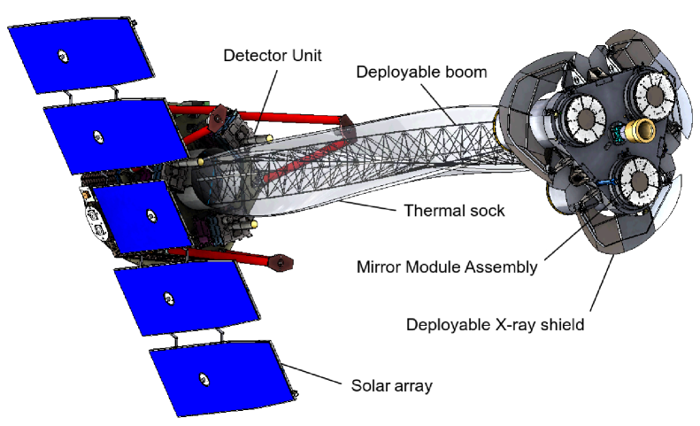
Figure 1.10: Illustration of the IXPE space observatory with the main instrumental parts described. Image from Di Lalla (2019).

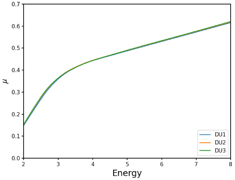
Figure 1.11: The GPD modulation factor $\mu(E)$ of DUs on board of IXPE at the time of launch. Image from Weisskopf et al. (2022).

We will elaborate on IXPE observations as part of the results in this dissertation, but let us provide one more detailed example of its capabilities. One may assume the average count rate for the IXPE observation of the X-ray bright accreting supermassive black hole in MCG-05-23-16 ($(0.525\pm 0.002)\,\textrm{counts}\cdot\textrm{s}^{-1}$ in 2–8 keV, Marinucci et al., 2022), where to obtain $M\!D\!P_{99\%}=4.7\%$ took 482 ks. If compared with the X-ray bright accreting stellar-mass black hole in Cygnus X-1 ($(40\pm 20)\,\textrm{counts}\cdot\textrm{s}^{-1}$ in 2–8 keV, Krawczynski et al., 2022), then, if similar observational time was given for Cygnus X-1, the same confidence limit for linear polarisation detection would be reduced to $M\!D\!P_{99\%}\approx 0.5\%$ for Cygnus X-1. These are extraordinary numbers, because polarimetry is in general photon-demanding when compared to spectroscopy or photometry. If the emission is e.g. $1\%$ polarized, we then require about 100 times more photons to process some information from the signal than a spectrograph counting each photon per the same band width would need, in order to be, generally speaking, as informative.

1.2.3 Science cases

X-rays are produced by vast number of sources in the Universe, such as planets, stars, ISM, stellar remnants, galaxies, galaxy clusters and gamma ray bursts (GRB) (Trümper and Hasinger, 2008). Out of these, X-ray polarimeters typically target objects with powerful acceleration mechanism, strong magnetic fields, possible presence of vacuum birefringence, strong gravity, and scatterings in aspherical geometries. During the first year and a half of operation, IXPE produced a number of interesting results when observing supernova remnants (Vink et al., 2022; Ferrazzoli et al., 2023; Zhou et al., 2023), pulsar wind nebulae (Xie et al., 2022; Bucciantini et al., 2023; Romani et al., 2023), the Sagittarius A* complex (Marin et al., 2023), GRBs (Negro et al., 2023), magnetars (Taverna et al., 2022; Turolla et al., 2023; Zane et al., 2023), accreting pulsars (Doroshenko et al., 2022; Marshall et al., 2022; Tsygankov et al., 2022; Doroshenko et al., 2023; Forsblom et al., 2023; Malacaria et al., 2023; Mushtukov et al., 2023; Suleimanov et al., 2023a; Tsygankov et al., 2023) and weakly magnetized accreting neutron stars (Capitanio et al., 2023; Chatterjee et al., 2023; Cocchi et al., 2023; Fabiani et al., 2023; Farinelli et al., 2023; Ursini et al., 2023a). The first IXPE observational results of accreting black holes will be summarized in Chapter 5.

1.3 Active galactic nuclei

From cosmological perspective, only a fraction of all galactic nuclei are active ($\lessapprox 40\%$, but the selection criteria are key, see e.g. Chiang et al., 2019), which means that there is a long-term, ongoing mass transfer from the surroundings onto the central supermassive black hole. Our Galaxy, for example, shows a very low activity at this epoch, but perhaps was strongly accreting in the past (Revnivtsev et al., 2004; Nobukawa et al., 2011; Chuard et al., 2018; Marin et al., 2023). The extreme power density, luminosity at all wavelengths, and rapid time variability of the active cores of galaxies caused a confusion in the 1950s on their origin, being first classified as “quasi-stellar astronomical radio-sources”, shortened as “quasars” (Chiu, 1964), by which we mean today a point-like UV or optical emitting object associated with a radio-source. With the development of radio astronomy, spectroscopy and interferometry in the 1960s, their true nature was revealed. Since 1970s and the development of gravitational lensing and high-resolution spectroscopy people are breaking records in finding active galactic nuclei (AGN) at higher and higher cosmological redshifts. At the time of writing of this dissertation, the furthest and oldest quasar is at redshift $z=7.642$, i.e. $\approx 670$ million years after the Big Bang, which challenges the structure formation theories within Big Bang cosmologies (Wang et al., 2021). Today we know that AGNs have diverse nature and dozens of classifications based on appearance at all wavelengths exist (see e.g. Pringle and Rees, 1972; Shakura and Sunyaev, 1973; Seward and Charles, 2010; Netzer, 2015).

If the host galaxy is identified, such galaxies with active nuclei are called “Seyfert galaxies”. They are named after Carl Seyfert (1911–1960), who first described this class already in 1943 (Seyfert, 1943). Probably the most useful distinction comes from the presence or absence of broad optical emission spectral lines in the cores of Seyfert galaxies, defined as “type-1” or “type-2” AGNs, respectively (Rowan-Robinson, 1977; Keel, 1980; Antonucci, 1993). A major breakthrough in understanding that these are actually one and the same axially symmetric objects, viewed under different inclination with respect to the axis of symmetry, came (not surprisingly) from polarimetry mostly in the 1980s (Dibai and Shakhovskoi, 1966; Walker, 1966; Angel et al., 1976; Antonucci, 1982, 1984; Antonucci and Miller, 1985). The so-called unification model (Antonucci, 1993; Urry and Padovani, 1995) assumes a nucleus with high orbital speeds of the infalling matter in equatorial disc structures, causing Doppler broadening of the spectral lines, that can be viewed bare from polar directions, but obscured from the sides. The cause of obscuration is accounted to a parsec-scale cold dusty torus residing in the equatorial plane. Infrared and X-ray observations suggest clumpy structure (Nenkova et al., 2002; Risaliti et al., 2002; Matt et al., 2003; Tristram et al., 2007) and elaborate spectral fitting shows large-scale geometries of the obscurer sometimes far from an actual geometrical torus (Fritz et al., 2006; Suganuma et al., 2006; Namekata et al., 2014; Siebenmorgen et al., 2015; Buchner et al., 2019; Ricci and Paltani, 2023). Although the size, shape, clumpiness and location of the obscuring material varies and is difficult to theoretically predict from the first principles, we know that its presence is related to the active state of inner black-hole accretion (Hopkins et al., 2012a; Schawinski et al., 2015).

Strongly magnetized accretion disc and the ergosphere in close vicinity of the black hole, arising from full GR description, may cause that some infalling material is ejected with relativistic speeds in polar directions through the so-called Blandford-Znajek or Blandford-Payne processes (Blandford and Znajek, 1977; Blandford and Payne, 1982; Rees et al., 1982; Blandford et al., 2019). The rich structures that can form around the poles reflect the central emission, which can thus gain polarisation through first-order scattering. The presence of broad lines in polarisation for type-2 AGNs unifies the picture (see e.g. Antonucci, 1993; Beckmann and Shrader, 2012; Seward and Charles, 2010). One can imagine the entire structure like the candle in Figures 1.13 and 1.13 viewed from the generic type-1 and type-2 directions, respectively. We also more specifically distinguish the clumpy equatorial broad line region (BLR) from the accretion disc located closer to the black hole and the torus itself, located further out. And if the clumpy regions extend at parsec scales vertically (in polar directions), we call them narrow line regions (NLR). It is also worth noting that perfect axial symmetry is often not the evolutionary case and some misalignment of the central black hole rotation axis from the accretion disc axis, misalignment of the disc plane from the distant equatorial obscurers, or misalignment of the dusty torus plane from the host galaxy plane, is considered (Bardeen and Petterson, 1975; Goosmann and Matt, 2011; Hopkins et al., 2012b; Tremaine and Davis, 2014; Stalevski et al., 2017; Chatterjee et al., 2020).

Figure 1.12: Photograph of a candle illustrating a type-1 view of an AGN. The wick is the central accretion engine, while the flame represents the polar jet that is often present.

Figure 1.13: The same as in Figure 1.13, but for a type-2 view. The central parts are obscured. Only for AGNs that are radio bright we identify polar ejecta of relativistic speeds.

Polar ejecta are often highly colimated (spanning only a few angular degrees from the black-hole poles) and represent perhaps the most energetic locations in the observable universe, hence called “jets”, often surrounded by more angularly extended ionization cones (see e.g. Peterson, 1997; Trümper and Hasinger, 2008; Seward and Charles, 2010; Blandford et al., 2019). Due to synchrotron emission, the jets are particularly bright in radio, leading to another very useful classification. If jets are present, which is in $10$–$20\%$ of AGNs (Kellermann et al., 1989; Peterson, 1997), we speak of “radio-loud” AGNs and “radio-quiet” AGNs are those with low jet activity. These relativistic streams of particles are remarkably stable and can outreach the entire host galaxy despite originating in the orders-of-magnitude smaller nucleus. Yet another theoretical challenge to high-energy astrophysicists. If the observer is looking straight into the narrow jet, we speak of a “blazar”, obviously showing very distinct observational traits from the rest of AGNs. In this dissertation, we will not cover blazars and we will focus on radio-quiet objects, not to complicate the already intricate story of X-ray polarisation origin due to synchrotron emission on top of scattering and absorption effects. In addition, AGNs possess more inclined winds originating from the accretion disc at more than a few gravitational radii (for recent reviews, see e.g. Proga, 2007; Czerny, 2019; Karas et al., 2021). These winds, significantly contributing to the total outflow rates and altering the central emission, are attributed to radiation, thermal or magneto-hydro-dynamical (MHD) driving mechanisms. Studying both jets and winds is also important for galaxy evolution theories that investigate the feedback of matter and radiation of AGNs with the host galaxies. One of the contemporary and ambitious unification diagrams (Beckmann and Shrader, 2012) with the major AGN constituents and some common classifications is shown in Figure 1.14. But we note that too detailed illustration can often cause a cognitive bias.

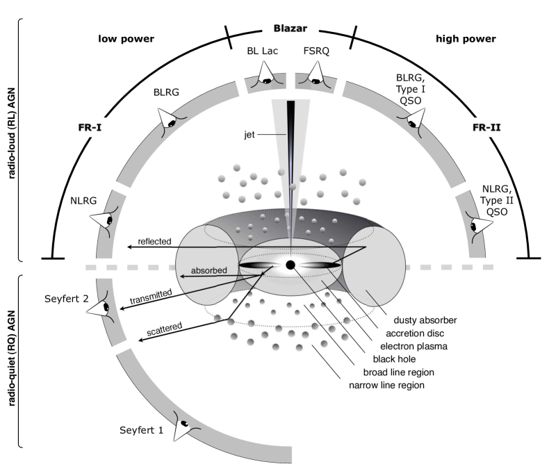
Figure 1.14: Schematic drawing of the AGN unification model and different nomenclature. Image from Beckmann and Shrader (2012).

The theory of black-hole accretion disc’s formation, stability and radiation properties is one of the most challenging parts of today’s astrophysics. Exact stable solutions to the governing Euler’s and Maxwell’s equations that would cover complicated microphysics are scarce (Abramowicz and Fragile, 2013). A practical analytical solution for a geometrically thin, optically thick disc was found by Shakura and Sunyaev (1973) and relativistically developed by Novikov and Thorne (1973); Page and Thorne (1974); Compère and Oliveri (2017). However, despite its remarkable utility for first-order estimates on radial structure and emission profile, it is often criticized for neglect of microphysics (described via ad hoc parameter $\bar{\alpha}$), instability and lack of support from observations and MHD simulations departing from the first principles (see e.g. Shakura and Sunyaev, 1976; Done et al., 1992; Abramowicz, 2005; Wang et al., 2014; Mishra et al., 2017; Zdziarski et al., 2022). Other famous, and perhaps more realistic solutions include discs of non-negligible size, which is related to the increased accretion rate and luminosity or increased advection to the detriment of radiative efficiency: the slim discs (Abramowicz et al., 1988), the “advection dominated accretion flows” (ADAF) (Narayan and Yi, 1994), the thick discs or Polish donuts (Jaroszynski et al., 1980), the puffy discs (Sądowski, 2016; Lančová et al., 2019), or combined descriptions, such as the “jet emitting disc standard accretion disc” (JED-SAD) model (Ferreira et al., 2006). The results of sophisticated MHD simulations that include GR effects and simplified radiative transfer are providing reasonably similar predictions with different codes (Porth et al., 2019), but in the current state of development they are difficult to be directly observationally validated. The intricate effects of thermal instabilities, convection and turbulences with respect to the vertical structure of the disc were studied, for example, by Agol et al. (2001); Turner (2004); Zhu and Narayan (2013).

For the sake of simplicity, we will be using the Novikov-Thorne model (i.e. the standard $\bar{\alpha}$-disc with relativistic corrections) for radial disc profiles, assuming Keplerian velocities, no torque on the inner boundary, and inner-disc radius extended to the inner-most circular orbit, if not stated otherwise. But we note that this might be one of the most critical model assumptions for the global emission predictions in Chapters 3, 4 and 5, difficult to assess unless a completely new model based on different assumptions is built.

In proper radiative transfer treatment of the accretion disc, we encounter another critical assumption for the result of mostly bound-bound and bound-free processes: the chemical composition and metallicity $A_{\textrm{Fe}}$, which sets the relative abundance of all ions with respect to some referential composition, typically that of our Sun (Matteucci, 2001). Various determinations of solar abundances relative to neutral hydrogen exist and are debated (Grevesse and Sauval, 1998; Asplund et al., 2005, 2009; Bergemann and Serenelli, 2014).

We define the Eddington luminosity $L_{\textrm{Edd}}$ as (e.g. Karas et al., 2021)

$$L_{\textrm{Edd}}=1.3\times 10^{46}\,\frac{M}{10^{8}\,M_{\odot}}\cdot\textrm{erg}\cdot\textrm{s}^{-1}$$ (1.35)

and the Eddington mass accretion rate $\dot{M}_{\textrm{Edd}}$ as (e.g. Karas et al., 2021)

$$\dot{M}_{\textrm{Edd}}=1.39\times 10^{18}\,\frac{M}{M_{\odot}}\cdot\textrm{g}\cdot\textrm{s}^{-1}\,.$$ (1.36)

They effectively describe the accretion state when radial radiative force balances the gravitational pull by the central body, which is referred to as Eddington limit. In these black-hole mass dependent units, we can then more conveniently discuss the true bolometric (or X-ray) luminosity $L_{\textrm{bol}}$ (or $L_{\textrm{X}}$) and mass accretion rate $\dot{M}$, which are proportional and which can be also observationally determined (see e.g. Davis and Laor, 2011). The geometrically thin and optically thick disc can be assumed to be locally thermally radiating as a black body, with a decreasing temperature profile with radius (Shakura and Sunyaev, 1973)

$$T_{\textrm{eff}}^{4}\sim\dfrac{\dot{M}}{\dot{M}_{\textrm{Edd}}}\left(\dfrac{r}{r_{\textrm{g}}}\right)^{-3}\dfrac{1}{M}\,,$$ (1.37)

hence forming a multicolor black-body spectrum, i.e. the “big blue bump” (Malkan, 1983; Czerny and Elvis, 1987). Although state-of-the-art radiative transfer equation solvers are able to treat the disc’s photosphere in great detail (see below), it appears difficult to capture the effects of Comptonization, which are to be assessed with next generation of codes (Shimura and Takahara, 1995a; Merloni et al., 2000; Davis et al., 2006; Done et al., 2012; Davis and El-Abd, 2019). Therefore, the empirical color correction factor $f_{\textrm{c}}$ (Ebisuzaki et al., 1984) is often used:

$$I=f_{\textrm{c}}^{-4}B(f_{\textrm{c}}T_{\textrm{eff}})\textrm{ ,}$$ (1.38)

where $B$ is from the Planck’s law (1.11). Typically AGN discs exhibit $n_{\textrm{H}}=10^{13}$–$10^{18}\ \textrm{cm}^{-3}$ and $T_{\textrm{eff}}=10^{3.5}$–$10^{6}\ \textrm{K}$, if the Novikov-Thorne model is assumed with observationally and theoretically motivated estimates of $1.5\lessapprox f_{\textrm{c}}\lessapprox 1.8$, $0.1\lessapprox\bar{\alpha}\lessapprox 0.2$, $10^{5}\lessapprox M/M_{\odot}\lessapprox 10^{9}$ and $0.01\lessapprox\dot{M}/\dot{M}_{\textrm{Edd}}\lessapprox 1$. The spectrum then peaks at the UV band for AGNs, which is well confirmed by observations (see e.g. Seward and Charles, 2010).

Lastly, let us focus more on the X-ray spectral properties of AGNs, for which they are undoubtedly famous. Examples of a broadband unfolded spectral energy distribution (SED) are shown in Figure 1.15. In the X-rays, we predominantly observe a decreasing power-law with energy $N\sim E^{-\Gamma}$, described by a power-law index $\Gamma$. This is a natural consequence of thermal disc emission Compton up-scattered in hot ($T_{\textrm{e}}\gtrapprox 10^{7}$ K) gas of electrons, the corona, located nearby (Shapiro et al., 1976; Liang and Price, 1977; Bisnovatyi-Kogan and Blinnikov, 1977; Sunyaev and Titarchuk, 1980; Haardt and Maraschi, 1991). The measured spectral slope is thus also related to the accretion rate and luminosity (e.g. Zdziarski et al., 1999; Lu and Yu, 1999; Wang et al., 2004; Risaliti et al., 2009; Brightman et al., 2013; Yang et al., 2015; Trakhtenbrot et al., 2017; Huang et al., 2020). The power-law is cut at hard energies (hundreds of keV) due to insufficient energy of the Comptonizing electrons. At the very hard (X$\gamma$) energy tail, electron-positron pair production and annihilation effects also play important role (Coppi and Blandford, 1990; Zdziarski et al., 1990; Coppi, 1999). But we decided to omit the relevant theoretical background in Section 1.1.2, because the models developed in this dissertation neglect these effects and operate at lower energy ranges. At soft energies (tenths of keV), the low-energy cut-off naturally appears due to the seed thermal photons energy, i.e. there are only a few scattered photons below some characteristic energy. Such coronae, which are inseparable part of the inner-most accreting regions, can be constrained up to some limit in terms of optical depth, electron temperature and geometry from spectroscopic and timing techniques (e.g. Haardt and Maraschi, 1991; Haardt, 1993; Haardt and Maraschi, 1993; Dove et al., 1997; Henri and Petrucci, 1997; Krolik, 1999; Ghisellini et al., 2004; Markoff et al., 2005; Dovčiak and Done, 2016; Kara et al., 2016; Fabian et al., 2017; Kara et al., 2017; Kubota and Done, 2018; Ursini et al., 2020). However, especially with geometry, which is a critical unknown, X-ray polarimetry has high potential in lifting the known degeneracies (Haardt and Matt, 1993; Poutanen and Svensson, 1996; Marinucci et al., 2018; Poutanen et al., 2018; Ursini et al., 2022; Krawczynski and Beheshtipour, 2022; Poutanen et al., 2023).

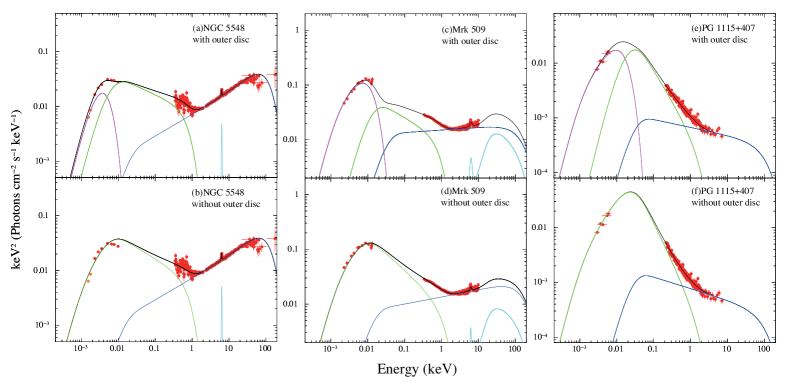
Figure 1.15: Broadband spectral energy distribution fit of various AGNs by Kubota and Done (2018). Details are provided therein. The fit consists of four distinct continua here: outer disc emission (in magenta), the warm Comptonized component (in green), and the hard Comptonized primary (in dark blue) and reflected (in light blue) components. Total unfolded spectrum is in black and the data from Mehdipour et al. (2011); Jin et al. (2012b, a); Mehdipour et al. (2015) in red. Panels (a), (b), (c), (d), (e) and (f) show fits of NGC 5548 with and without outer disc, Mrk 509 with and without outer disc and PG 1115+407 with and without outer disc, respectively. Image from Kubota and Done (2018).

In the literature, one finds many realizations for the coronal geometry and bulk motion. Although non-stationarity of the primary source is sometimes considered (Beloborodov, 1998, 1999; Beloborodov and Poutanen, 1999; Malzac et al., 2001; Poutanen et al., 2023), we will assume a stationary situation in this dissertation, which affects the polarisation properties due to negelect of some potential aberration effects. The most simplified phenomenological model is the “lamp-post model” (e.g. Matt et al., 1991; Martocchia and Matt, 1996; Henri and Petrucci, 1997; Petrucci and Henri, 1997; Martocchia et al., 2000; Miniutti and Fabian, 2004; Dovčiak et al., 2004b, 2011; Parker et al., 2015; Fürst et al., 2015; Miller et al., 2015; Niedźwiecki et al., 2016; Dovčiak and Done, 2016; Walton et al., 2017; Ursini et al., 2020) that assumes a point-like isotropic X-ray emitter located on the rotation axis at some height above the black hole. Although this model is difficult to support from photon conservation point of view and Comptonization codes always require at least a minimal spatial extension of the corona, it may serve as a prototype for an optically thin aborted jet or base of a jet with spherical, or perhaps more favored conical shape. Of completely different emission properties are “extended coronal models” (e.g. Haardt and Maraschi, 1991; Haardt, 1993; Poutanen and Svensson, 1996; Dabrowski and Lasenby, 2001; Malzac et al., 2005; Niedźwiecki and Życki, 2008; Schnittman and Krolik, 2010; Marinucci et al., 2018; Poutanen et al., 2018), where the corona is diffuse and elongated in equatorial direction. These range from sandwich models, where the corona forms only a geometrically thin layer on the disc, to wedge models, to large spherical models engulfing the entire inner-accreting region. These are considered both patchy and with uniform density. Last, distinct archetype is the “hot inner-accretion flow” (Poutanen and Svensson, 1996; Dove et al., 1997; Esin et al., 1997, 1998; Zdziarski et al., 1998; Liu et al., 2007; Poutanen and Vurm, 2009; Veledina et al., 2013b; Poutanen et al., 2018) that does not assume the hot gas above and below the disc, or in the polar directions, but rather in wedge-like or cylindrical geometries inside the accretion disc, if truncated at significant distance from the event horizon and with debatable role of synchrotron seed photons. Although the evidence and direct knowledge about X-ray emitting coronae is coming primarily from X-ray observations, some deeper theoretical support is provided from plasma simulations for the emergence of coronae and its heating, using the kinetic approach (and less from plasma fluid simulations), but determining the geometry anyhow would be a significant step forward for this field (e.g. Begelman et al., 1983; Begelman and McKee, 1983; Di Matteo, 1998; Wilkins and Fabian, 2012; Beloborodov, 2017; Nättilä and Beloborodov, 2022; Liska et al., 2022; El Mellah et al., 2022; Bambic et al., 2024).

X-ray spectra of radio-quiet AGNs may contain also a strong reflection component of the X-ray power-law originating in the hot corona (e.g. Guilbert and Rees, 1988; Lightman and White, 1988; Fabian et al., 1989; Matt et al., 1993; Fabian et al., 2000; Reynolds and Nowak, 2003; García et al., 2013). In continuum, we typically see a Compton shoulder at about 20 keV that is caused by interplay of Compton down-scattered photons with nearly constant mid-X-ray cross-section with energy and photoelectric absorption with comparable, but decreasing cross-section as $\sim E^{-3}$. Many emission lines appear on top of the continuum, especially below 2 keV and in the iron line complex near 6–7 keV. If these lines are narrow, we ascribe this reflection to the torus, distant disc or other components far-away from the central accretion engine. If broad, then these are assumed to be relativistically smeared and originating in reflection off inner accretion disc close to the black hole or in the winds (see Parker et al., 2022b, for the discussion of degeneracy between the two). The relativistic reflection component in both line and continuum features enables independent spectroscopic and timing determinations of the black-hole spin, coronal geometry, source orientation and the accretion disc’s properties (see Reynolds, 2019, and references therein). The anticipation is that X-ray polarimetry can independently constrain such properties (Rees, 1975; Connors and Stark, 1977; Stark and Connors, 1977; Connors et al., 1980; Dovčiak et al., 2004a, 2008; Schnittman and Krolik, 2009; Li et al., 2009; Marin, 2014; Cheng et al., 2016; Marin, 2016; Taverna et al., 2020, 2021; Ursini et al., 2022; Krawczynski and Beheshtipour, 2022; Mikušincová et al., 2023). A theoretical X-ray reflection spectrum from a constant-density plane-parallel disc in the local comoving frame is shown in Figure 1.17 for different values of the ionization parameter, which is, regarding the presence of main spectral features, supported by larger number of AGN observations (e.g. Gottwald et al., 1995; Winter et al., 2009; Ng et al., 2010). Fabian et al. (2000) discusses four distinct regimes of the spectral dependence on $\xi$. For a given density, the higher the impinging bolometric flux is, the less continuum absorption and emission lines we see, and the disc acts as a highly reflective Compton mirror to the original power-law. The reflected power-law can also return to the disc due to strong gravity and reflect again, multiple times, which affects both spectra and polarisation, depending for example on the spin of the black hole and coronal parameters (Schnittman and Krolik, 2009, 2010; Connors et al., 2021; Dauser et al., 2022).

Figure 1.16: Theoretical AGN X-ray reflection spectrum for various values of the ionization parameter $\xi$ defined by (1.18). The more the disc is ionized, the more the reflected spectrum resembles the original power-law. Image from Fabian et al. (2000).

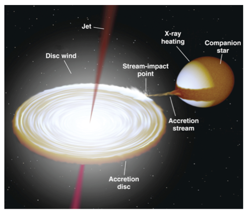
Figure 1.17: Artist’s impression of the XRB system, including the indication of main components. The accretion disc surrounding the stellar-mass black hole is formed by a stream of matter from the companion star. Image from Fender and Belloni (2012), courtesy of Rob Hynes.

Disentangling the AGN X-ray spectra is a difficult task due to large multiplicity in the observed power-law spectra (Trümper and Hasinger, 2008; Seward and Charles, 2010). The soft X-rays of AGNs are further complicated by the presence of the “soft X-ray excess”, for which competing explanatory theories exist until today. The most promising being the warm corona model, or that this feature is a natural extension of the big blue bump located in the UV or that it appears due to a presence of broad spectral lines (e.g. Boroson and Green, 1992; Boller et al., 1996; Pariev and Bromley, 1998; Branduardi-Raymont et al., 2001; Lee et al., 2002; Gierliński and Done, 2004; Mehdipour et al., 2011; Różańska et al., 2015; Kubota and Done, 2018; Petrucci et al., 2020). Across all X-rays, we also observe variability in emission and absorption (on shorter time scales than viscous characteristic times) due to flares, cloud eclipses, warm absorbers and winds inside the system, or due to absorption in the host galaxy or in the ISM of our Galaxy (e.g. Halpern, 1984; Nandra and Pounds, 1994; Peterson, 1997; Porquet and Dubau, 2000; Porquet et al., 2004; Trümper and Hasinger, 2008; Seward and Charles, 2010). For data fitting, absorption is typically characterized through one parameter along the entire line of sight: the neutral hydrogen column density $N_{\textrm{H}}\ [\textrm{cm}^{-2}]$ (see e.g. the TBABS model, Wilms et al., 2000).

1.4 X-ray binary systems

Multiple gravitationally bound stellar systems are more common than solitary stars in the Universe (Duchêne and Kraus, 2013). Interesting configurations may occur over the life-time of a binary stellar system, resulting in increased X-ray brightness. We will focus on X-ray bright binary systems in stable mass transfer evolutionary phase with stellar-mass black hole as an acceptor, and a giant or supergiant ordinary star as a donor. These are called black-hole X-ray binary systems (XRB) and the brightness at all wavelengths (not only X-rays) is given much through the same mechanisms as in the quasars, including the presence of the disc-corona-jet system (Rees, 1998; Done et al., 2007; Seward and Charles, 2010). Hence, these are often nicknamed as “microquasars” (Mirabel et al., 1992). In XRBs, the mass transfer happens through Roche lobe (in XRBs with low mass of the donor) or additionally through stellar winds of the donor (with high-mass donor star). Sketch of the entire stellar binary system is shown in Figure 1.17. Due to radiation effects combined with the formed gravitational potential well, the accretion disc is formed with overall higher mean effective temperatures ($T_{\textrm{eff}}=10^{5}$–$10^{7.5}\ \textrm{K}$) and neutral hydrogen densities ($n_{\textrm{H}}=10^{19}$–$10^{25}\ \textrm{cm}^{-3}$) compared to AGNs. This again theoretically follows from the Novikov-Thorne disc solution, assuming orders-of-magnitude lighter central black hole ($M=6$–$20\,M_{\odot}$, Reynolds and Nowak, 2003). This is important for our modeling, because the peak of the multicolor black-body radiation is well within the soft X-rays, which is observationally confirmed (see e.g. Gierliński et al., 1999). The growing observational evidence of high-density accretion discs in XRBs is a recent success of modern X-ray spectral fitting models of reflected disc emission (García et al., 2016; Tomsick et al., 2018; Jiang et al., 2019b, a, 2020; Connors et al., 2021; Liu et al., 2023), although many of these studies assume a constant and extreme density even in the upper layers of the disc atmosphere, which is a debatable simplification. Because of the additional significant presence of the thermal component in the X-rays and because of the expected high disc densities, we will first develop models suitable for AGNs, which seems in principle a less ambitious task, and then try to adapt them to XRBs.

However, it may be easier to deduce observationally relevant information on accretion physics with XRBs, not only due to their X-ray brightness compared to AGNs, which is critical for photon-demanding polarimetry (see Section 1.2.2). At human time scales, the nature was perhaps more favorable to us with XRBs than AGNs, because stellar-mass black holes can change their accretion state in periods of months or years, thus we can arguably infer more on their accreting nature (Fender et al., 2004). Some transient sources show unstable outbursts with eight to nine orders of magnitude difference in luminosity across day periods with most significant distinction in the X-rays (see e.g. Connors et al., 2021). The change of state is best characterized in the so-called Q-diagram of X-ray flux ratios, which is depicted in Figure 1.18. XRBs show hysteresis evolution in hardness-intensity diagram, often evolving from the prototypical “low/hard state” to the “high/soft state” and back (see Zdziarski and Gierliński, 2004; Remillard and McClintock, 2006, and references therein). The former is characterized by bright coronal emission compared to thermal emission from the disc, significant disc truncation and strong presence of jets. The latter is characterized by dominant thermal component, accretion disc reaching to the ISCO and jets being switched off. An extensive nomenclature for intermediate or irregular states exists. A broadband spectral energy distribution fit of different X-ray spectral states of high-mass XRB Cyg X-1 is shown in Figure 1.20. An example of modelled decomposition of the soft state of Cyg X-1 is shown in Figure 1.20.

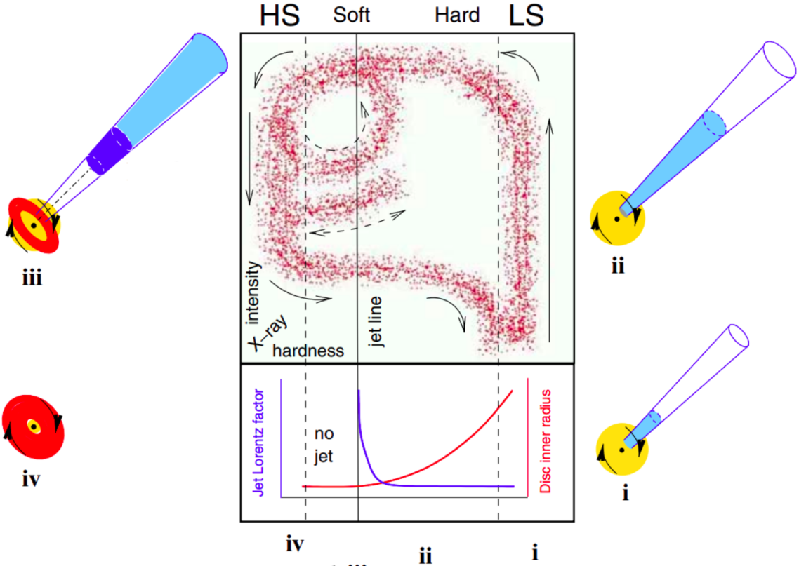
Figure 1.18: Schematic drawing of the XRB spectral states in the X-ray hardness-intensity diagram. The evolution of a typical binary system follows a hysteresis behavior in the shape of a letter “Q”. However, many sources exhibit irregularities and operate in just part of the configuration space. The two most extreme states, the low/hard state (LS on the picture) and the high/soft state (HS on the picture), vary by jet presence and theoretical inner disc radius. Image adapted from Fender et al. (2004).

Figure 1.19: Broadband fitted spectral energy distribution of the soft, intermediate and hard XRB states of Cygnus X-1 by Gierliński et al. (1999). The models are hybrid, consisting of the thermal disc component, a hard power-law continuum component and a broad power-law reflection component. The data were taken between 1991 and 1996 by the Ginga, RXTE, ASCA and OSSE instruments. Image from Gierliński et al. (1999).

Figure 1.20: The soft state from the same study as in Figure 1.20 by Gierliński et al. (1999) with spectral decomposition shown. A thermal black-body contribution in the X-rays is visible, alongside a harder reflection component accompanying the primary power-law coronal contribution. Image from Gierliński et al. (1999).

The XRB spectral, timing and polarisation characteristics of the corona and outflows related to accretion are similar to those of AGNs and we refer to the literature in Section 1.3, which is in many cases applied to XRBs. The characteristics of stellar winds and circumbinary obscuring material depend on the evolutionary phase of the binary system, which in turn is largely given by the initial mass of both components, eccentricity, separation or orbital period (Tauris and van den Heuvel, 2006). The dusty torus as in AGNs is not forming, because the accreting matter is streamed directly from the nearby orbiting companion. Short-term variability in absorption and emission is observed similarly to AGNs. If the binary orbital axis is misaligned with the black hole spin axis, the inner accretion disc may become warped, which may be also linked to the Lense-Thirring precession phenomenon (Lense and Thirring, 1918; Bardeen and Petterson, 1975; Stella and Vietri, 1998; Fragile et al., 2007; Abarr and Krawczynski, 2020). This effect is imprinted in light curves of many wavelengths as quasi-periodic oscillations (QPO) (Ingram et al., 2009; Veledina et al., 2013a).

People tried with moderate success to identify in AGNs the spectral states observed in XRBs, tied in theory to the accretion mechanism, although in AGNs they should occur at larger time scales, thus observable only statistically (Körding et al., 2006; Svoboda et al., 2017; Fernández-Ontiveros and Muñoz-Darias, 2021; Moravec et al., 2022). Without doubt, better understanding of the accretion disc itself would significantly move up all AGN and XRB branches of studies. Albeit decades of intensive research, it proved to be a challange. It is perhaps desirable to aim at particular subproblems, such as determination of the inner disc radius, which is important for both theoretical and observational consideration of accreting black holes (see e.g. Krolik and Hawley, 2002; Seward and Charles, 2010): particularly in understanding and putting constraints on the GR effects, disc theories, MHD simulations, multiwavelength spectroscopy, reverberation mapping, QPO studies, and last but not least, X-ray polarisation outlook of inner-accreting regions, which we will explore in this dissertation.

1.5 Computational approach

In Sections 1.3 and 1.4, we focused on the observational and physical description of accreting black holes, integrating all obtained knowledge. Apart from X-ray polarisation, we focused on their X-ray spectral properties, because any polarisation simulation must adequately produce and cross-validate the Stokes parameter $I$ too, even if not in high precision.

Timing properties were not of key interest from X-ray polarimetric point of view, thus we omitted the summary of relevant literature. Long-term changes expected in X-ray polarisation of accreting black holes are typically described through different slowly evolving configurations of static polarisation models. The only exceptions being orbital-phase-resolved polarisation analysis of XRBs and a possibility of detecting QPOs in polarisation. The former is interesting from the point of view of changing geometry of reflection from the stellar wind, reflection from the stellar companion or periodic eclipses. The latter could be seen in associated quasi-periodic changes in the polarisation angle due to misalignment of the inner disc part, as it precesses. Regarding short-term variability caused by e.g. corotating flares or clouds with the accretion disc, one can estimate the typical Keplerian orbital periods around Kerr black holes from Bardeen et al. (1972), which are negligibly short compared to typical observational time needed with IXPE to obtain a polarisation detection of XRBs or fainter AGNs (cf. Section 1.2.2). We obtain $\approx 10\,\textrm{ms}$ orbital period at $10\,r_{\textrm{g}}$ for a stellar-mass black hole with $M=10\,M_{\odot}$ and $\approx 10\,\textrm{ks}$ orbital period at $10\,r_{\textrm{g}}$ for a supermassive black hole with $M=10^{7}\,M_{\odot}$. Thus, with instruments such as IXPE, we observe a rotationally smeared signal from the inner-accreting regions.

The numerical methods used and developed in this work are built on the shoulders of decades of intensive modeling by various research groups. We will now introduce the literature on the X-ray spectropolarimetric modeling of the studied (static) systems. We will first summarize the main findings of the past, and then give technical background of this work, making use of the elementary processes outlined in Section 1.1 and having in mind the practical motivations illustrated in Section 1.2.

1.5.1 Modeling of environments near black holes

Typically, MHD or kinetic plasma simulations that are able to grasp a large region near black hole self-consistently (see e.g. Nättilä and Beloborodov, 2022; Liska et al., 2022; Wielgus et al., 2022; Liska et al., 2023) do not treat radiative transfer in sufficient depth or are too computationally expensive to provide trustworthy observational interpretation via direct data fitting and case-to-case interpolation. For this reason, we rather use for specific problems radiative transfer equation solvers, MC simulations, or fully analytical models that tend to be the most computationally efficient. We note that recently, machine learning techniques were used in X-ray studies of AGNs or XRBs not only for faster classification of collected data (Hebbar and Heinke, 2023) or reducing spectral fitting time (Parker et al., 2022a), but also for increasing modeling resolution by means of interpolating computationally expensive models computed in a few grid points at majority of the parameter space and in high density at a smaller region of the parameter space that was used as a training set (Matzeu et al., 2022).

Analytical approximations provided perhaps the most classical results in the second half of $20^{\textrm{th}}$ century. Chandrasekhar provided estimates on polarisation due to Rayleigh single-scattering in reflection from plane-parallel slab (Chandrasekhar, 1960), which we will often use. For unpolarized primary radiation (in transcription from Dovčiak, 2004)

$$I =\dfrac{I_{\textrm{l}}+I_{\textrm{r}}}{\langle I_{\textrm{l}}+I_{\textrm{r}}\rangle}I_{\textrm{N}}\textrm{ ,}$$ (1.39)

$$Q =\dfrac{I_{\textrm{l}}-I_{\textrm{r}}}{\langle I_{\textrm{l}}+I_{\textrm{r}}\rangle}I_{\textrm{N}}\textrm{ ,}$$

$$U =\dfrac{\hat{U}}{\langle I_{\textrm{l}}+I_{\textrm{r}}\rangle}I_{\textrm{N}}\textrm{ ,}$$

$$V =0\textrm{ ,}$$

where

$$I_{\textrm{l}} =\mu_{\textrm{e}}^{2}(1+\mu_{\textrm{i}}^{2})+2(1-\mu_{\textrm{e}}^{2})(1-\mu_{\textrm{i}}^{2})-4\mu_{\textrm{e}}\mu_{\textrm{i}}\sqrt{(1-\mu_{\textrm{e}}^{2})(1-\mu_{\textrm{i}}^{2})}\cos(\Phi_{\textrm{e}}-\Phi_{\textrm{i}})\textrm{ ,}$$

$$\textrm{ }-\mu_{\textrm{e}}^{2}(1-\mu_{\textrm{i}}^{2})\cos[2(\Phi_{\textrm{e}}-\Phi_{\textrm{i}})]\textrm{ ,}$$

$$I_{\textrm{r}} =1+\mu_{\textrm{i}}^{2}+(1-\mu_{\textrm{i}}^{2})\cos[2(\Phi_{\textrm{e}}-\Phi_{\textrm{i}})]\textrm{ ,}$$

$$\hat{U} =4\mu_{\textrm{i}}\sqrt{(1-\mu_{\textrm{e}}^{2})(1-\mu_{\textrm{i}}^{2})}\sin(\Phi_{\textrm{e}}-\Phi_{\textrm{i}})-2\mu_{\textrm{e}}(1-\mu_{\textrm{i}}^{2})\sin[2(\Phi_{\textrm{e}}-\Phi_{\textrm{i}})]\textrm{ ,}$$

where

$$\Phi_{\textrm{i}}=-R_{\textrm{sgn}}^{\textrm{i}}\arccos\left(\dfrac{-1}{\sqrt{1-\mu_{\textrm{i}}^{2}}}\dfrac{p_{\textrm{i}\alpha}e_{(\phi)}^{\alpha}}{p_{\textrm{i}\mu}U^{\mu}}\right)+\dfrac{\pi}{2}$$

and $R_{\textrm{sgn}}^{\textrm{i}}$ is the sign of the radial component of the four-momentum $p_{\textrm{i}}^{\mu}$ of an incident photon. It is positive if the incident photon travels outwards ($p_{\textrm{i}}^{(r)}>0$), and negative, if it travels inwards ($p_{\textrm{i}}^{(r)}<0$) in the local rest frame of the disc. The rest of the angles describe the reflection event with respect to the disc’s normal and photon’s incident and emergent direction: $\mu_{\mathrm{i}}$ is the cosine of incident inclination angle $\delta_{\textrm{i}}$ measured from the disc’s normal, $\mu_{\mathrm{e}}$ is the cosine of emergent inclination angle $\delta_{\textrm{e}}$ (in Section 1.1.3 considered as $n_{\textrm{em}}$, in Chapter 2 will be sometimes considered as the global $\theta$) measured from the disc’s normal, $\Phi_{\mathrm{e}}$ is the relative azimuthal angle measured counter-clockwise at the disc plane between the emission and the incident ray directions projected to the disc’s surface. For unpolarized primary, if the results are integrated in $\mu_{\textrm{i}}$ and $\Phi_{\textrm{e}}$, the resulting polarisation fraction monotonically increases with inclination from $0\%$ up to about $20\%$ and the polarisation angle is parallel with the slab. We refer the reader to Chandrasekhar (1960) for prescriptions for polarized primary and for the result for diffuse pure-scattering reflection with the assumption of infinite scatterings.

The semi-infinite plane-parallel atmosphere was also approached by Chandrasekhar and Sobolev in transmission problem (Chandrasekhar and Breen, 1947; Sobolev, 1949; Chandrasekhar, 1960; Sobolev, 1963), where the pure-scattering result is displayed in Figure 1.22. The Loskutov-Sobolev approximation (Loskutov and Sobolev, 1981) is also displayed for comparison, which takes into account additional effect of absorption, which increases polarisation due to effectively reduced symmetry: the photon paths are most likely vertical towards the slab surface, providing a preferred scattering angle for an observer at given inclination (Lightman and Rybicki, 1979; Loskutov and Sobolev, 1979). In addition, it accounts for internal sources within the atmosphere, which typically depolarize due to smaller mean free path through the atmosphere compared to the classical Milne problem, where the sources are located only at the bottom of the atmosphere (Milne, 1921; Loskutov and Sobolev, 1981). The details depend on the source function distribution with optical depth and the ratio of scattering to absorption opacities. In some cases, the vertical gradient of thermal source function can additionally polarize (Harrington, 1969; Gnedin and Silant’ev, 1978; Loskutov and Sobolev, 1979; Bochkarev et al., 1985). And already Nagirner (1962) pointed out that the emergent polarisation angle may not always be parallel to the slab, if internal sources of radiation are considered and the result resembles an optically thin limb brightened atmosphere (Gnedin and Silant’ev, 1978; Matt et al., 1993; Davis et al., 2009).

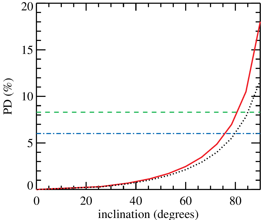
Figure 1.21: Polarisation fraction versus observer’s inclination for transmission through semi-infinite atmosphere in pure-scattering limit (black dotted, Chandrasekhar, 1960) and with absorption and internal sources of radiation (red solid, Loskutov and Sobolev, 1981). The latter is also parametrized by the ratio of scattering coefficient to the sum of scattering and true absorption coefficients, which gives higher polarisation for smaller values of the ratio. The horizontal lines correspond to IXPE data of XRB system 4U1630-47, see Ratheesh et al. (2024) for details. Image from Ratheesh et al. (2024).

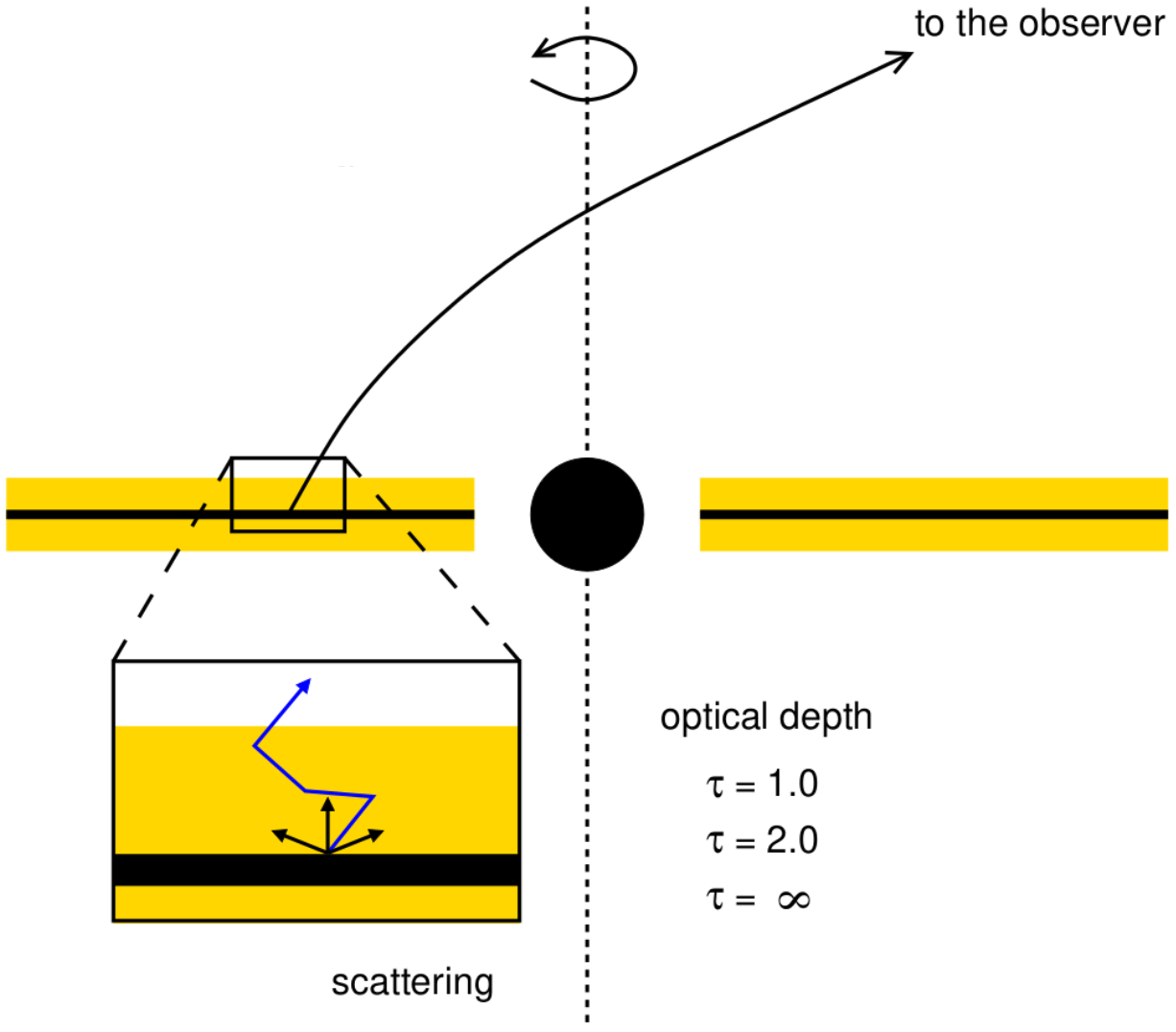
Figure 1.22: Model of thermally radiating geometrically thin disc around Kerr black hole. The atmosphere is approximated in local comoving frame by slab of some optical depth $\tau$. In the most simple approach, we can assume the optical depth of $\tau\rightarrow\infty$ and only scattering events of thermal radiation reaching upwards. Once we precalculate the emission escaping the semi-infinite atmosphere, we switch to GR ray tracing from equatorial plane towards an observer under general inclination $\theta$ with respect ot the principal axis, which coincides with the Boyer-Lindquist coordinate $\theta$. Image courtesy of Michal Dovčiak.

For the pure-scattering semi-infinite atmosphere in transmission, numerical solution to the guiding integro-differential equations is tabulated in e.g. Chandrasekhar (1960), but a useful empirical law can be used (Viironen and Poutanen, 2004):

$$p=-\frac{1-\mu_{\textrm{e}}}{1+3.852\mu_{\textrm{e}}}11.71\%\,,$$ (1.40)

describing the monotonic increase with energy up to about $12\%$. The emergent polarisation angle is parallel to the disc in this case, as usual for scattering-dominated limb darkened atmospheres. The semi-infinite atmosphere with large absorption can be approximated by (1.15) or (1.17) with polarisation angle parallel to the slab for photons emerging at large atmospheric depths and scattering once at the disc surface plane with scattering angle $\Theta$ coinciding with observer’s inclination $\theta$ with respect to the disc’s normal. Without the effects of absorption, the multiple scattering events for transmission through finite plane-parallel slab were studied by Sunyaev and Titarchuk (1985) with the resulting polarisation parallel to the slab for large optical thickness, but perpendicular for Thomson optical depth $\tau_{\textrm{T}}\lessapprox 3$, depending on the inclination angle. For optically thin case, the single-scattering approximation gives (Sunyaev and Titarchuk, 1985)

$$p=\frac{1-\mu_{\textrm{e}}^{2}}{3-\mu_{\textrm{e}}^{2}}\,,$$ (1.41)

reaching $33\%$. The function (1.41) is monotonically decreasing with $\mu_{\textrm{e}}$ and less steeply than in (1.40). The corresponding polarisation is parallel to the projected slab normal, i.e. orthogonal to the scattering-induced polarisation vector from a semi-infinite atmosphere. Polarisation by single scatterings from general axially symmetric structures was in exact form described by Brown and McLean (1977).

Modern analytical or semi-analytical codes focus for example on the X-ray polarisation arising from neutral or fully ionized disc, when illuminated by the coronal power-law, on two-phase coronae with relativistic electrons, or self-consistent treatment of the disc and corona, including multiple scattering orders and synchrotron radiation in particular geometries, or outflowing coronae with relativistic velocities that affects polarisation due to aberration effects (Bonometto et al., 1970; Dolginov et al., 1970; Gnedin and Silant’ev, 1978; Silant’ev, 1979; Williams et al., 1984; Williams, 1984; Sunyaev and Titarchuk, 1985; Matt, 1993; Haardt and Matt, 1993; Poutanen and Vilhu, 1993; Nagirner and Poutanen, 1993; Poutanen and Svensson, 1996; Poutanen et al., 1996; Beloborodov, 1998; Nagirner and Poutanen, 2001; Silant’ev and Alexeeva, 2007; Bianchi et al., 2010; Poutanen and Vurm, 2010; Silant’ev et al., 2018, 2020, 2021, 2022; Veledina and Poutanen, 2022; Loktev et al., 2022; Nagirner et al., 2022; Nagirner and Grachev, 2022; Silant’ev et al., 2023; Poutanen et al., 2023; Loktev et al., 2023; Dexter and Begelman, 2024). The works of Poutanen and Svensson (1996); Veledina and Poutanen (2022) introduced a spectral fitting COMPPS model, which has also a polarisation extension, but the extension is currently not available in interface with XSPEC [private communication with the authors].

The optically thick atmosphere for X-ray reflection or transmission with internal source distribution was numerically treated by many authors (either via radiative transfer equation solving or via MC methods) for the X-ray photospheres of black-hole accretion discs. For plain spectral output for example by Mitsuda et al. (1984) (the DISKBB model for fitting of simple multicolor thermal disc emission), or Kříž and Hubený (1986); Hubeny and Hubeny (1997, 1998); Davis et al. (2005); Davis and Hubeny (2006) (relativistically integrated thermal discs in hydrostatic equilibrium and the BHSPEC model), or Suleimanov (1992); Suleimanov et al. (2002, 2007) (similarly), or Shimura and Takahara (1993, 1995b, 1995a) (similarly), or Li et al. (2005) (the KERRBB model for relativistic thermal disc emission), or Ross and Fabian (1993); Matt et al. (1993a); Ross et al. (1999); Ross and Fabian (2005, 2007) (the REFLIONX models for power-law reflection from constant density discs), or Magdziarz and Zdziarski (1995); Zdziarski et al. (1996); Życki et al. (1999) (the PEXRAV and PEXRIV models for power-law reflection from neutral and fully ionized constant-density disc, respectively, and the NTHCOMP model for Comptonized power-law), or Kallman and Bautista (2001); García and Kallman (2010); García et al. (2011, 2013, 2016, 2020) (the XSTAR code and XILLVER models for local power-law constant-density reflection), or Różańska and Czerny (1996); Nayakshin et al. (2000); Nayakshin and Kallman (2001); Péquignot et al. (2001); Ballantyne et al. (2001); Dumont et al. (2002); Różańska et al. (2002); Dumont et al. (2003); Różańska and Madej (2008); Różańska et al. (2011); Vincent et al. (2016) (the NOAR, TITAN and ATM24 codes and comparisons of both constant-density and hydrostatic equilibrium power-law reflection), or Mehdipour et al. (2011); Różańska et al. (2015); Petrucci et al. (2020); Gronkiewicz et al. (2023) (the radiative transfer treatment of warm coronal emission in AGNs), among others.

Analytical or numerical treatment of locally radiating geometrically thin disc atmosphere is typically implemented into a GR ray tracing code, such as Dovčiak et al. (2004a, b, 2008, 2011); Taverna et al. (2020, 2021); Dovčiak et al. (2022); Mikušincová et al. (2023) (the KY codes applied to various different computations of emission in local comoving frame with the disc for various geometries, see below), or García et al. (2014); Dauser et al. (2014, 2022) (the RELXILL code for relativistic lamp-post extension to XILLVER tables, currently being developed also to treat various coronal geometries), or Niedźwiecki et al. (2016); Niedźwiecki and Zdziarski (2018); Niedźwiecki et al. (2019) (spectral relativistic lamp-post models), all building on the older works of e.g. Fabian et al. (1989); Laor (1991); Matt and Perola (1992); Matt et al. (1992, 1993b, 1996b); Agol (1997); Martocchia et al. (2000); Beckwith and Done (2004). Figure 1.22 illustrates such relativistic embedding for thermally radiating geometrically thin discs, but similar sketch is applicable to the local disc reflection integration for geometrically thin discs. Slim disc models with relativistic extensions, suitable for observational fitting of e.g. ultra luminous X-ray sources (ULX) – compact objects accreting in super-Eddington regime –, were constructed by Kawaguchi (2003); Straub et al. (2011); Vierdayanti et al. (2013); Caballero-García et al. (2017), among others.

We will compare our spectral results to some of the above studies to validate our more unique polarisation results, because numerical radiative transfer computations of X-ray polarisation near accreting black holes are scarce due to the complexity of the problem. We name the early works of Stark (1981); Phillips and Meszaros (1986); Nagendra and Peraiah (1987); Matt et al. (1989); Laor et al. (1990); Coleman and Shields (1990, 1991); Matt et al. (1991, 1993); Matt (1993); Agol and Blaes (1996); Blaes and Agol (1996); Matt et al. (1996c); Hsu and Blaes (1998); Agol et al. (1998); Lee (1999); Agol and Krolik (2000); Silant’ev (2002) and then more recently Dovčiak et al. (2004a); Gnedin et al. (2006); Silant’ev and Gnedin (2008); Dovčiak et al. (2008); Li et al. (2009); Davis et al. (2009); Schnittman and Krolik (2009); Dovčiak et al. (2011); Marin and Tamborra (2014); Silant’ev et al. (2019a, b); Taverna et al. (2020, 2021) for the geometrically thin disc in transmission or reflection with various simplified assumptions, or combined with coronal contribution in selected geometries by Schnittman and Krolik (2010), or for geometrically thick discs in the attempt by West and Krawczynski (2023) and warped discs by Cheng et al. (2016); Abarr and Krawczynski (2020). Particularly relevant to this dissertation (to be discussed in depth later) is the lamp-post relativistic reflection of polarisation computed in Dovčiak et al. (2011) in simplified approach and the non-relativistic total polarisation gained by scattering and absorption of thermal disc emission computed by combined approach of radiative transfer solver CLOUDY (Ferland et al., 2013, 2017) with MC simulator STOKES (Goosmann and Gaskell, 2007; Marin et al., 2012, 2015; Marin, 2018), described in Taverna et al. (2021). In the neighboring field of accreting neutron stars, where often the role of magnetic fields is more critical, much theoretical progress motivated by the IXPE observations is also seen (e.g. Sokolova-Lapa et al., 2021; Suleimanov et al., 2023b; Sokolova-Lapa et al., 2023). Lastly, there are two exceptional X-ray polarisation codes that focus on the Comptonization treatement in coronae with MC method, including GR effects in Kerr spacetime. The MONK code (Zhang et al., 2019b, 2022, 2023) is predicting the X-ray polarisation outcome for coronae of various geometries with seed photons from the disc and MC treatment of inverse Compton scattering in the corona. Perhaps of even more complexity, also including GR effects, is the KerrC code (Krawczynski and Beheshtipour, 2022), which calculates also reflection from the accretion disc. Recently, another MC spectropolarimetric attempt for computation of coronal emission was obtained by Kumar (2024). Although some of these MC computations involve peculiar effects of partial ionization, or radiation returning to the disc, there are always some admittable simplifications to the detriment of detailed radiative transfer. A notable relativistic MHD simulation providing X-ray polarisation predictions was done by Schnittman et al. (2016) and in Moscibrodzka (2023), linked to a MC code.

A specific category is the modeling of cold distant components of AGNs, where large libraries of torus X-ray spectral models exist (see e.g. Liu and Li, 2014; Furui et al., 2016; Buchner et al., 2019; Vander Meulen et al., 2023, and references therein). These are typically separated from the inner disc-corona system computations and assume such external (central) source of emission. From polarisation perspective, these are easier to be treated by MC codes than radiative transfer equation solvers. We name the works of Ghisellini et al. (1994); Matt et al. (1996a); Ursini et al. (2023b) and Goosmann and Matt (2011); Marin et al. (2012, 2016, 2018a, 2018b); Ursini et al. (2023b) for dusty tori and polar outflows of uniform density, and pioneering attempts for X-ray polarisation signatures of clumpy obscurers by Marin et al. (2012, 2013, 2015). These could be perhaps accompanied in the future by results with the MC code SKIRT (Baes et al., 2011; Baes and Camps, 2015; Camps and Baes, 2015, 2020; Vander Meulen et al., 2023) that is currently developing polarisation effects in the X-rays, similarly to STOKES [private communication with the authors]. However, some ambitious radiative transfer equation solvers that include X-ray polarisation estimate have been performed to evaluate the warm absorbers in AGNs (Dorodnitsyn and Kallman, 2010, 2011). Many of these models can be also applied to the obscuring funnels of XRBs, ULXs, or accreting neutron stars or white dwarfs, which can be formed by vertically extended outflows or the accretion disc itself (e.g. Poutanen et al., 2007; Wielgus et al., 2016; Narayan et al., 2017; Koljonen and Tomsick, 2020; Neilsen et al., 2020; Miller et al., 2020; Ratheesh et al., 2021; Doroshenko et al., 2023). Recently, analytical treatment of this problem also emerged in Veledina et al. (2023b) and Tomaru et al. (2024) attempted for X-ray polarisation MC modeling of polarisation of incident black-body emission of soft-state XRBs gained by scattering in optically thin thermal-radiative winds, implementing polarisation into the MONACO code (Odaka et al., 2011). The latter was followed by Tanimoto et al. (2023), which modelled the X-ray polarisation specifically in the obscured Circinus Galaxy, using the MC MONACO code linked to radiative hydrodynamic simulations.

1.5.2 Codes explored in this dissertation

We will now elaborate a bit more on the numerical codes and models adopted for new results produced within this dissertation.

TITAN

TITAN (Dumont et al., 2003) is a non-LTE radiative transfer code suitable for studying X-rays in hot photoionized media, such as atmospheres of accretion discs. It solves the energy balance, the ionization equilibria and the statistical equilibria (1.20) and the transfer equation in a plane-parallel geometry (1.19), all for the lines and continuum up to about $26\textrm{ keV}$. The iterative method is the accelerated lambda iteration (ALI) (Cannon, 1973; Scharmer, 1981; Olson et al., 1986; Hubeny, 2003), ideal for fast convergence in spectral lines. In the latest version 105v03f that we use, TITAN was updated for many atomic transitions (Adhikari et al., 2015; Goosmann et al., 2016). In total $\approx 4000$ X-ray spectral lines are considered. We will use the code for studying the radiative problem of a plane-parallel disc atmosphere in order to obtain the ionization structure, i.e. fractional abundance of each ion. Although TITAN allows other enclosing relations, we will use it for a constant density atmosphere only. TITAN does not have polarisation computations implemented and its treatment of Comptonization is simplistic. It should not be used for densities $n_{\textrm{H}}\gtrapprox 10^{18}\,\textrm{cm}^{-3}$ with the atomic data and treatment of collisions that is available [private communication with the authors].

STOKES

STOKES is a 3D MC simulator suitable for media where scattering and absorption are the dominant sources of opacity. The code is ideal for studying polarisation, because many critical line and continuum processes are implemented. Although various usage exists (Marin and Goosmann, 2014; Marin and Grosso, 2017), it was primarily developed to study AGNs in the optical and UV, and more recently the code expanded to X-rays (version 2.07 onwards). It includes the effects of Compton down-scattering on free electrons, using the Klein-Nishina cross section (1.13) and proper energy redistribution (1.12), but the angular redistribution is treated according to Thomson phase functions (see Section 1.1.2). Then it includes scattering on bound electrons and dust (including dust absorption), the bremsstrahlung absorption and emission (in emission for spectral lines only, i.e. the resonant bremsstrahlung; the free-free continuum emission is not implemented yet), and photoelectric absorption. It solves for several thousands of spectral lines. Polarisation due to resonant line scattering is treated according to Lee (1994); Lee et al. (1994); Lee and Blandford (1997). The competing Auger effect is also implemented. On the other hand, as an MC code it cannot consistently solve for the ionization structure, temperature and magnetic fields. The densities and temperatures of the scattering and absorbing regions have to be predefined and are used for various processes. But for example the thermal emission or synchrotron radiation have to be included as external input emitters, in case of need. In the latest version (from v2.34 onwards), which was developed simultaneously with this dissertation and hence will not be used, STOKES also includes the inverse Compton scattering according to Poutanen and Vilhu (1993) with predefined temperature information. Although we will not use it, STOKES also allows for the treatment of circular polarisation, time variability and velocity of scattering regions.

The code allows for arbitrary polarisation of the emission originating in predefined emission regions (directional or undirectional). We will use the notation $p_{0}$, $\Psi_{0}$ for the incident polarisation degree and angle of a photon that is to be reprocessed. The energy distribution of the primary radiation input can be self-defined or based on templates. A weighting algorithm is implemented to prevent cumulation of numerical noise in one part of the resulting spectrum. The scattering regions, which can coincide with emission regions, allow for non-trivial geometries (planar layers, cones, wedges etc.) and practical symmetry reductions, as MC simulations are known for large computational costs. Inside the scattering region, each photon can be either scattered (including true absorption and immediate reemission) or absorbed (and thermalized, although thermal reemission is neglected) with some probability $P_{\textrm{X}}$. This is computed according to exponential probability law at distance $d$ travelled inside the scattering region with cross-section $\sigma_{\textrm{X}}$ for each process with particle species of uniform density $n_{\textrm{X}}$:

$$P_{\textrm{X}}=e^{-n_{\textrm{X}}\sigma_{X}d}\textrm{ .}$$ (1.42)

The polarisation modification upon each reprocessing event is treated using the Müller formalism. Although the photon cannot be emitted out of nothing outside of the emission region (e.g. through thermal radiation), the emission region can overlap with the scattering region. If the photon escapes the scattering medium and reaches a detector in particular predefined angular and energy binning, the polarisation information is transformed into the global reference frame and registered, including renormalized flux information. Additional routine ANALYZE developed by the same authors is used to convert the raw output to conveniently readable files with the Stokes parameters per energy and angular bins of the detectors.

We will use STOKES for computations of reflection and transmission in plane-parallel atmospheres, where we will combine the MC approach with TITAN to precompute ionization structure of vertically stratified layers properly. This will be in depth described in Chapter 2. Apart from that, we will also use STOKES alone for computation of distant reflection in partially ionized equatorial and polar obscurers in Chapter 4. There we will assume homogeneous media in various simplified geometries and shrink the entire disc-corona emitting system to a point in the center of coordinates.

KY

Lastly, let us focus again on the modeling of the inner-accreting regions and the necessary inclusion of relativistic effects. To solve the polarized radiative transfer in vacuum according to the layout sketched in Section 1.1.3, we will use and adapt the well-tested KY codes. There are numerous KY routines available for solving of polarized radiative transfer in Kerr space-time: from solving of relativistically smeared spectral lines (Dovčiak et al., 2004a, b; Dovčiak, 2004) (including convolution models), to thermal radiation emitted from the disc (Dovčiak et al., 2008; Taverna et al., 2020, 2021; Mikušincová et al., 2023), to coronal emission added with simplified reflection from the disc (Dovčiak et al., 2011) and broadband spectra of lamp-post coronae with simplified reflection and thermalized continuum (Dovčiak et al., 2022). All of these codes depart from the principles sketched in Section 1.1.3 and all relativistic effects are taken into account, apart from returning radiation. Returning radiation is not implemented yet to the codes apart from the KYNBBRR routine (Taverna et al., 2020; Mikušincová et al., 2023), computing total disc thermal emission for a distant observer, which allows for simplified returning radiation effects, using albedo parameter $0\leq A\leq 1$ and reflecting the same spectropolarimetric energy distribution of photons. Although we provided the main results in Section 1.1.3 in the most commonly known Boyer-Lindquist coordinates, the KY codes solve (1.22), (1.23) and (1.25) in the so-called Kerr ingoing coordinates for numerical purposes (Misner et al., 1973; Dovčiak et al., 2004a). Symmetry of the coronal geometries adopted allow for largely simplified treatment of radiation in between the corona and the disc, in between the corona and the observer and in between the disc and the observer. The code produces unfolded Stokes parameters for a distant observer (1.26), renormalized for a general source distance $r_{0}=1$ Mpc.

In this dissertation, we will adapt the lamp-post and extended coronal geometries and the associated reflection routines KYNLPCR and KYNXILLVER, which use the local spectral reflection tables from NOAR and XILLVER codes and polarized reflection given by single-scattering Chandrasekhar’s formulae (1.39) (Dovčiak et al., 2011; Marin et al., 2018a, b). A sketch of the two simplified disc-corona setups explored is in Figure 1.23, including the parametrization. As previously described, the inner-accreting regions will be essentially computed in two different phases. First, we will compute locally the reflection or transmission with TITAN and STOKES, assuming a semi-infinite atmosphere, which will be described in Chapter 2. Then, we will assume a global view where GR radiative transfer in vacuum with KY is applied on a geometrically thin disc, which will be described in Chapter 3. Hence, the precomputed semi-infinite atmosphere in tabular format will be used as infinitely geometrically thin in the second step, following the essentials of the Novikov-Thorne accretion theorem. Assuming such two distinct local and global scales that can be computationally separated, we inexpensively combine detailed radiative transfer inside the critical top layers of the disc, simplified accretion physics and relativistic effects.

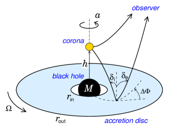
Figure 1.23: Two model geometries of a corona above an accretion disc: a) the lamp-post model, b) the extended coronal model. The main model parameters are labeled. Images from Dovčiak (2004); Dovčiak et al. (2014).

For the lamp-post model, we will assume an isotropically emitting point-like corona at height $h$ above the center of the black hole (ranging in principle from the event horizon all the way to relativistically nearly “flat” regions beyond $100\,r_{\textrm{g}}$). Local reflection in comoving frame with the accretion disc can be then described by the previously defined three angles $\mu_{\textrm{i}}=\cos{\delta_{\textrm{i}}}$, $\mu_{\textrm{e}}=\cos{\delta_{\textrm{e}}}$, $\Phi_{\textrm{e}}$ [see (1.39) and Figure 1.23 for a sketch]. For the combined signal with the primary emission we also have to specify the scaling of primary to reflected flux $N_{\textrm{p}}/N_{\textrm{r}}$, which in the model is unity for self-consistent treatment of corona with a given isotropic luminosity $L/L_{\textrm{Edd}}$ and reflection fraction according to the local reflection tables. The extended corona is not parametrized by height, as we assume it is geometrically thin and glued at the top of geometrically thin disc, i.e. still within the black-hole equatorial plane. However, we have to define a radial profile of ionization, given by a power-law index $q$ and the ionization parameter normalization $\xi_{0}$:

$$\xi=\xi_{0}r^{-q}\,.$$ (1.43)

The KY codes allow integration of smaller sections of the disc given by $r_{\textrm{in}}$, $r_{\textrm{out}}$ and $\phi_{\textrm{min}}$, $\Delta\phi=\phi_{\textrm{max}}-\phi_{\textrm{min}}$ boundaries, in order to compute the effects of partial obscuration and flares. We will only work with radial disc truncation in this dissertation, due to the aforementioned insensitivity of current X-ray polarimeters to short-term variability in the accretion flow. The codes also allow for global redshift $z$ and time dependent treatment of emission, which we will not use in this work. The same holds for non-constant radial profile of the disc’s density.

Chapter 2 Emission from a partially ionized accretion disc in a local comoving frame

This chapter describes modeling of local accretion disc emission in plane-parallel approximation, either through reflection or transmission. No SR or GR effects are assumed. We assume a passive plane-parallel atmosphere comoving with the source of illuminating radiation.

2.1 Power-law reflection off a disc’s atmosphere

We begin with the results of reflection of a coronal power law from a constant-density slab of high optical thickness held in photoionization equilibrium. We use the combination of TITAN and STOKES (v2.32) codes, which allows for accurate treatment of partial ionization effects. Because TITAN is not equipped with polarisation computations, we couple it to STOKES, which is built for accurate polarisation treatment. Conversely, the STOKES MC simulation cannot solve self-consistently for the ionization structure, thus an iterative solver like TITAN is required for detailed studies of hot X-ray photoionized media. The core of the presented model was already achieved as part of Podgorný (2020), including normalization and production of the final model tables in Flexible Image Transport System (FITS) format (Hanisch et al., 2001) and a brief discussion. We examined and cross-validated the resulting spectropolarimetric tables as part of this dissertation in greater detail, which is summarized in Podgorný et al. (2022, 2023a). In addition to these publications and the older tables used there, a new version was recently created. This version contains only two changes: (i) a unified grid in $\xi$, which was in all previous publications not available (we worked with different $\xi$ values per each $\Gamma$) due to a technicality, and (ii) $100\%$ vertically polarized illumination for those tables that were previously computed for $100\%$ horizontally polarized illumination. The tabular model is now ready-to-use for manipulation in XSPEC, as the FITS files with unified $\xi$ conform to Office of Guest Investigator Programs (OGIP) standard (Arnaud, 1995) of XSPEC.

Table 2.1 describes the current parameter values, for which also the results below are drawn and which are physically motivated. Each model table contains one Stokes parameter and is computed for $100\%$ vertically polarized ($p_{0}=1$, $\Psi_{0}=0^{\circ}$), $100\%$ diagonally polarized ($p_{0}=1$, $\Psi_{0}=45^{\circ}$), and unpolarized ($p_{0}=0$) incident radiation. Three incident polarisation states allow immediate interpolation for arbitrary polarisation state that will be used in Section 3. The source of primary radiation is located directly above the slab. Each table was computed for $N_{\textrm{tot}}=7\times 10^{8}$ simulated photons, which is sufficient for investigating the elementary spectral and polarisation properties with negligible presence of inevitable MC numerical noise.

Table 2.1: Description of the FITS tables representing the local reflection tables computed, which were recently updated for ionization parameter grid that does not depend on $\Gamma$.

Number of tables	9 (vertical, diagonal, and no incident polarisation
	versus the $I$, $Q$, $U$ output)
Stokes parameters units	$[\textrm{counts}\cdot\,\textrm{cm}^{-2}\cdot\,\textrm{s}^{-1}]$
Energy range	$0.1\textrm{ keV}$ to $100\textrm{ keV}$
Energy binning	300 bins, $\Delta\log E=0.01$
$\Gamma$	{$1.4,1.6,1.8,2.0,2.2,2.4,2.6,2.8,3.0$}
$\xi$ $[\textrm{erg}\cdot\textrm{cm}\cdot\textrm{s}^{-1}]$	{$5,10,20,50,100,200,500,1000,2000,5000,10000,$
	$\ \ \ 20000$}
$\mu_{\mathrm{i}}$	{$0.0,0.1,0.2,0.3,0.4,0.5,0.6,0.7,0.8,0.9,1.0$}
$\mu_{\mathrm{e}}$	{$0.025,0.075,0.175,0.275,0.375,0.475,0.575,$
	$\ \ \ 0.675,0.775,0.875,0.975$}
$\Phi_{\mathrm{e}}$	{$7.5^{\circ},22.5^{\circ},37.5^{\circ},52.5^{\circ},67.5^{\circ},82.5^{\circ},97.5^{\circ},$
	$\ \ \ 112.5^{\circ},127.5^{\circ},142.5^{\circ},157.5^{\circ},172.5^{\circ},187.5^{\circ},$
	$\ \ \ 202.5^{\circ},217.5^{\circ},232.5^{\circ},247.5^{\circ},262.5^{\circ},277.5^{\circ},$
	$\ \ \ 292.5^{\circ},307.5^{\circ},322.5^{\circ},337.5^{\circ},352.5^{\circ}$}
Extensions	Primary Header – description of the tables
	‘PARAMETERS’ – parameter values
	‘ENERGIES’ – low and high energy bin edges
	‘SPECTRA’ – values of the Stokes parameters and
	corresponding model parametric values

The results were obtained for neutral hydrogen density $n_{\textrm{H}}=10^{15}\ \textrm{cm}^{-3}$; hence, the main application are accretion discs of AGNs. This is different from the follow-up section on X-ray thermal radiation passing through a disc’s atmosphere, which is clearly applicable to XRBs and which was studied for a range of slab densities. The reflection is computed up to Thomson optical depth of $\tau_{\textrm{T}}=\sigma_{\textrm{T}}n_{\textrm{H}}H=\sigma_{\textrm{T}}\times 10^{25}\ \textrm{cm}^{-2}\approx 7$, where $H$ is the total geometrical thickness of the slab studied. No radiation source is considered on the opposite side. The solar abundance is from Asplund et al. (2005) with $A_{\textrm{Fe}}=1$, neglecting the presence of dust. The high and low-energy cut-offs of the primary power-law were considered exponential in TITAN (for the computation of the ionization structure) and sharp in STOKES (for the computation of spectropolarimetric properties), cut at $E_{\textrm{min}}=10^{-1.1}\,\textrm{keV}\,\approx 0.079$ keV and $E_{\textrm{max}}=10^{2.4}\,\textrm{keV}\,\approx 251.189$ keV. We used angle-averaged illumination in TITAN for technical reasons, but we note that the vertical ionization structure should be incident angle dependent if pencil-like beams were studied, which leaves some deficiency on the results in terms of accuracy at high optical depths.

A much larger simplification with respect to real atmospheric conditions is the assumption of constant density. When studying the reflection in full hydrostatic equilibrium, well-known thermal ionization instability occurs along with narrow two-phase zones in the medium between the disc and the corona (see e.g. Begelman et al., 1983; Różańska and Czerny, 1996), even though the detailed geometry and boundary conditions of the illuminated atmosphere are unknown (Ballantyne et al., 2001; Ross and Fabian, 2005, 2007). Reflection from slabs in hydrostatic equilibrium were previously studied from spectroscopic point of view, but comparisons to constant-density models are scarce, as there is no ionization parameter defined for the former case and it is difficult to define an average atmospheric density (Różańska et al., 2002). It is however clear that the two classes of models vary in both continuum shapes and spectral line profiles (Nayakshin et al., 2000; Nayakshin and Kallman, 2001; Péquignot et al., 2001; Ballantyne et al., 2001; Różańska et al., 2002; Dumont et al., 2002; Ross and Fabian, 2007; Różańska and Madej, 2008; Różańska et al., 2011; Vincent et al., 2016). It is unclear how refraining from the constant-density assumption would quantitatively affect the polarisation properties of the emergent spectra, which are of our prime interest, as they have not been numerically computed with detailed treatment of partial ionization before neither in hydrostatic equilibrium, nor assuming constant density. Qualitatively, however, we know that if the upper atmospheric layers are heated, they expand and due to lower density their ionization level increases; and on the contrary the ionization level significantly drops below the instability point (Nayakshin et al., 2000; Done and Nayakshin, 2007; Done, 2010). For a full hydrostatic equilibrium, we would thus expect a shift of polarisation towards the highly ionized computations shown below for a constant density case.

2.1.1 Spectropolarimetric properties

Figure 2.1 shows the reprocessed spectra, polarisation degree versus energy and polarized flux for various $\xi$ values, three emission inclination angles $\delta_{\textrm{e}}$ and for unpolarized primary with $\Gamma=2$. The results are integrated in incident inclination angles $\delta_{\textrm{i}}$ and emergent azimuthal angles $\Phi_{\textrm{e}}$, in order to gain higher energy resolution in polarisation and in order to approximate the situation of an emitting disc observed under inclination $\delta_{\textrm{e}}$ with no GR or SR effects. In the spectra, we obtained the characteristic photon redistribution by disc reprocessing. We see the Compton hump at around 20 keV, the most prominent iron line complex at 6–7 keV and a forest of lines below 2 keV. The spectral shape changes with ionization according to the literature (compare with e.g. Figure 1.17, adopted from Fabian et al., 2000).

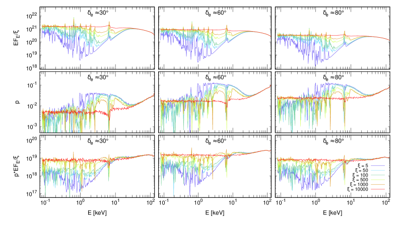
Figure 2.1: The locally reprocessed emission of the unpolarized incident power-law in the constant-density atmosphere, as computed by TITAN and STOKES and angle-averaged in $\delta_{\textrm{i}}$ and $\Phi_{\textrm{e}}$. The color code corresponds to different values of the ionization parameter $\xi$ $[\textrm{erg}\cdot\textrm{cm}\cdot\textrm{s}^{-1}]$. We show the values of $\mu_{\mathrm{e}}=0.875,0.475,0.175$ (left to right panels, $\delta_{\mathrm{e}}=28.96^{\circ},61.65^{\circ},79.92^{\circ}$). Top row: the spectra corrected for the slope of primary irradiation $\Gamma=2$ and divided by $\xi$ to account for amplitude differences. Middle row: the corresponding polarisation degree versus energy. Bottom row: the corresponding polarized flux, i.e. the values in the top row multiplied by the values in the middle row.

In polarisation, we obtained depolarisation in spectral lines and the continuum changes according to the (multiple-)scattering and absorption opacity contributions. The higher the absorption, the higher the single-scattering contribution is and the geometry is effectively reduced to dominant single-scattering angles. We see almost energy-independent polarisation for the cases with highest ionization with lack of emission lines. The polarisation is generally order-of-magnitude lower from the tabular FITS values, which are not integrated in $\delta_{\textrm{i}}$ and $\Phi_{\textrm{e}}$. This is because in particular incident and emission angle combinations with $\Theta\approx 90^{\circ}$ as the dominant single-scattering angle, the polarisation can easily reach values close to unity, while the angle-averaged results mean vectorial addition of many individual polarisation directions, hence depolarisation. Multiple scatterings also generally depolarize, because any leading directionality is washed out. We observe a reverse imprint of the spectral Compton hump in polarisation due to depolarisation by multiple scatterings. At the hard energy tail, we see increase in polarisation, because the Compton down-scattering energy redistribution results in more scatterings per emerging photon towards the lower energies. And in general, the photons penetrate deeper in the slab for smaller $\delta_{\textrm{i}}$. In deeper layers the matter is less ionized and more absorbing, so the vertical stratification diminishes the depolarisation (and photon energy change) by multiple scatterings for those photons that reached deep inside and emerged unabsorbed. We would, however, require a combined simulation of the photosphere for thermally radiating inner disc (in the X-rays more relevant for XRBs than AGNs) and power-law reflection from the other side of the atmosphere (see e.g. Różańska et al., 2011) to properly account for ionization, temperature and density structure closer to the disc mid plane. This is left for future studies and the produced reflection tables should be thus used rather for AGN accretion discs.

Despite the accurate treatment of polarisation in resonantly scattered lines in STOKES (Lee, 1994; Lee et al., 1994; Lee and Blandford, 1997), we do not see any gain of polarisation in spectral lines, as is observed e.g. in Dorodnitsyn and Kallman (2010, 2011) for the problem of AGN warm absorbers. However, more detailed investigation of polarisation in individual spectral lines would require higher spatial and energy resolution.

The flux and polarisation in hard X-rays would obtain a slightly different shape, if Comptonization was included. Qualitatively, we expect an effect of smoothing out the hard-energy spectral tail and slight decrease of polarisation due to additional photon energy shifts (Poutanen and Vilhu, 1993; Krawczynski et al., 2011; García et al., 2020). We estimate that for the studied slab temperatures ($T\approx 10^{7}$ K) this would begin to play a role at $\gtrapprox 10$ keV (Prince, 2004) (i.e. above the IXPE range), but a comparison with results using the latest version of STOKES v2.34 is still awaited. Polarisation through inverse Compton scattering is also related to the synchrotron emission, which emerges in optically thin media and is expected to be low for optically thick accretion discs.

The angle-averaged polarisation angle is in all cases $\Psi\approx 90^{\circ}$ and constant in energy (apart from the unpolarized fluorescent spectral lines, for which the default polarisation angle is undefined). The constancy with energy holds even for individual local reflection tables, although, depending on the local disc normal, the energy-independent value may differ with respect to individual rays studied (see below).

The dependency on inclination of the spectra follows from reflection limb darkening, as more photons are absorbed in the disc surface direction. The polarisation is known to increase with inclination on the contrary, because if the observer is looking at the reflecting surface pole-on, the individually polarized beams cancel out in polarisation from directions symmetric around the disc normal. The most prominent rise in polarisation degree occurs up to $\theta\approx 60^{\circ}$. An observer that would be further inclined sees similar polarisation in the Newtonian picture, while the average flux keeps decreasing towards the edge-on viewing angles. Hence, the polarized flux reaches maximum at $\theta\approx 60^{\circ}$, which suggest the most favorable inclination for detection of X-ray polarisation generated by plain disc reflection. The polarized flux panels not only support the antagonistic behavior of the flux and polarisation degree with energy, but symbolize the original Stokes parameters $Q=Ip\cos{2\Psi}$ and $U=Ip\sin{2\Psi}$ without any sign oscillations (because the continuum of $\Psi$ is constant in energy), again abstracted away from the slope and amplitude changes.

From spectroscopic point of view, an interesting quantity is the disc’s reflectivity, which is considered in thermal reverberation disc-corona studies, where it is assumed that a fraction of X-ray coronal radiation is absorbed and thermalized (Kammoun et al., 2019; Dovčiak et al., 2022). We will plot it here as the number of photons $N_{\textrm{r}}$, which are unabsorbed and reprocessed into all directions (i.e. integrated in $\delta_{\textrm{e}}$ and $\Phi_{\textrm{e}}$) divided by the total number of inserted photons $N_{\textrm{tot}}$ in the final STOKES MC simulation. Apart from changing the slope of the reflected radiation, higher values of $\Gamma$ increase the presence of spectral lines in our reprocessed emission tables, similarly to the effects described in García et al. (2013) for XILLVER computations. If integrated in energy and in incident inclination angle $\delta_{\textrm{i}}$, which only slightly increases reflectivity due to higher fraction of photons unabsorbed in the deeper atmospheric layers, the total reflectivity then rises with both $\Gamma$ and $\xi$, forming a characteristic “S” shape with $\xi$ for low $\Gamma$. This is displayed in Figure 2.3 as another perspective of the well-known reflection spectral change with $\xi$.

The dependency of the reflected spectra on incident polarisation is negligible. The dependency of the reflection-induced polarisation on the incident polarisation is substantial for individual combinations of {$\delta_{\textrm{i}},\delta_{\textrm{e}},\Phi_{\textrm{e}}\}$, but if angle-averaged, it becomes of the order of incident polarisation degree. We will examine this dependency in detail altogether with GR effects for a distant observer in Section 3. The cases of $100\%$ polarized radiation modelled locally here are by itself “unphysical” in a sense that they were computed in order to subsequently interpolate for realistic low values ($p_{0}\lessapprox 10\%$, Beheshtipour et al., 2017; Beheshtipour, 2018; Tamborra et al., 2018; Ursini et al., 2022; Krawczynski and Beheshtipour, 2022) of coronal polarisation.

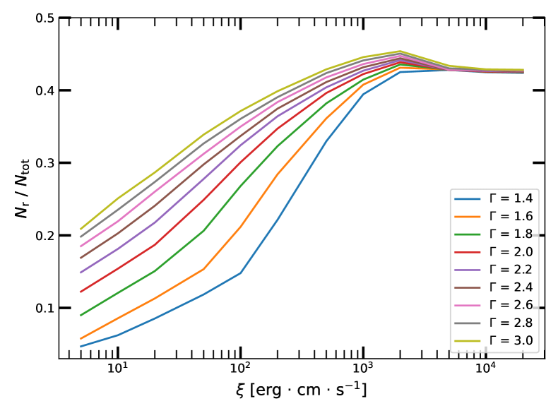
Figure 2.2: The $\xi$-dependency of the fraction of reflected photons with respect to the number of incident photons in the total energy range studied, integrated in incident inclination angle $\delta_{\textrm{i}}$. The color code corresponds to different values of $\Gamma$.

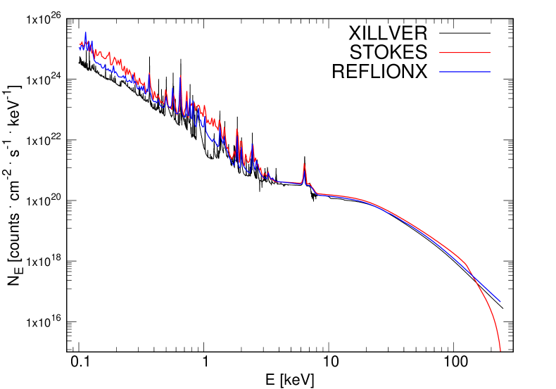
Figure 2.3: Comparison of spectra for $\Gamma=2.2$ and $\xi=100\,\,\textrm{erg}\cdot\textrm{cm}\cdot\textrm{s}^{-1}$, as computed by the XILLVER model (black), REFLIONX model (blue) and TITAN and STOKES for unpolarized primary (red), all normalized accordingly and angle-averaged.

2.1.2 Comparison to other models

In this section, we directly juxtapose the spectra of XILLVER, REFLIONX and our model for the same $\xi$ and $\Gamma$, although a thorough comparison between our model and the available constant-density spectral reflection tables would be also needed in terms of the used cut-offs, abundances or reflectivity. We overlap the three spectral models in Figure 2.3 for one case of $\xi$ and $\Gamma$ and in Figure A.1 in Appendix A for a few other examples at various corners of the parameter space. The necessary angle averaging and renormalization of the three models was done according to the procedures described in Podgorný (2020); Podgorný et al. (2022), which proves the correct analytical transformation of the STOKES output to physical units of our model stored in the FITS files described by Table 2.1. The results computed with TITAN and STOKES are generally closer to the REFLIONX tables than to the XILLVER tables. The same slab densities are assumed.

Without extensive investigation we can only state general reasons for possible discrepancies, but we note that even the differences between the widely used REFLIONX and XILLVER tables are poorly understood (García et al., 2013). The majority of the disagreement lies in the soft X-rays where many spectral lines occur and the spectra are more sensitive to the cut-off selection and abundances (cf. the comparisons between XILLVER and PEXRAV and PEXRIV in García et al., 2013, where also the largest dissimilarities occur at soft X-rays). The abundances used for REFLIONX are from Morrison and McCammon (1983) and for XILLVER are from Grevesse and Sauval (1998), i.e. more outdated to our model (see the discussion in Grevesse et al., 2007), but in García et al. (2013) it is argued that the choice of atomic data does not noticeably affect the result. There are, however, at least two times more X-ray spectral lines considered in XSTAR, forming the basis of the XILLVER tables, than in TITAN. Also, the XILLVER tables were computed up to $\tau_{\textrm{T}}=10$, which may result in higher accuracy. We note that the resolution of current X-ray polarimeters is far beyond resolving individual spectral lines and our model is motivated by numerical simulation of polarisation, it should not be used for accurate spectral data fitting.

At hard X-rays, the spectra are nearly identical. We stress that our MC results were obtained by a completely different numerical method than XILLVER with XSTAR, which simultaneously solves the equations of radiative transfer, energy balance, and ionization equilibrium in a Compton-thick, plane-parallel medium, using the Feautrier method (Mihalas, 1978), or REFLIONX, which utilizes the Fokker-Planck diffusion equation, including a modified Kompaneets operator (Ross et al., 1978; Ross, 1979). The fact that in mid and hard X-rays we reach a good agreement is favorable for the current and forthcoming X-rays polarimeters operating at these energy ranges, but less favorable for bringing more clarity in unveiling the nature of the spectral soft excess in AGNs. The inclusion of all three $\delta_{\textrm{i}}$, $\delta_{\textrm{e}}$ and $\Phi_{\textrm{e}}$ angles in our model should be an advantage over the other for a subsequent detailed disc integration in curved space-time. This is even more important for polarisation, which is more sensitive to geometry than pure spectra.

An attempt was made to cross-validate the latest model by using the code CLOUDY for ionization structure precomputations instead of TITAN, and then to use STOKES in the same manner. It was concluded that the CLOUDY code, originally designed for much lower density environments and temperatures, is on its limits for the X-ray power-law reflection problem and the mechanisms inside the code are poorly understood to produce a trustworthy reference. The intermediate results of this experiment were forwarded to the group of Roberto Taverna who were more successful in constructing models of thermally radiating XRB disc atmospheres with CLOUDY and STOKES (Taverna et al., 2021), which we will discuss in the next section.

To cross-validate the emergent polarisation from TITAN and STOKES, we used the Chandrasekhar’s single-scattering analytical approximation (1.39), which was used e.g. in Dovčiak et al. (2011) to estimate the net polarisation from disc reflection for a distant observer. We discovered however a sign error in these local reflection formulae when transcripted for Dovčiak et al. (2011), which was described and corrected in the appendix B of Podgorný et al. (2023a). To provide a direct comparison of the Chandrasekhar’s approximation with our model at 10–100 keV (with no lines and polarisation gained almost entirely by Compton recoil), we plot in Figure 2.4 the polarisation degree and angle for unpolarized primary versus various angular combinations of {$\delta_{\textrm{i}},\delta_{\textrm{e}},\Phi_{\textrm{e}}\}$. Compton multiple down-scatterings that are treated by STOKES depolarize the output in some cases by almost $50\%$ with respect to the value given by single Rayleigh scattering events. If only single-scattered photons are registered in STOKES, the results differ by just $\approx 1.5\%$ in the emergent polarisation degree. The results are symmetric in $\Phi_{\textrm{e}}$ around $180^{\circ}$, as expected. The angular dependency of our numerical simulation follows that of the Chandrasekhar’s, which is reassuring from the code implementation point of view. Especially for the emergent polarisation angle, which is highly sensitive to the scattering geometry and which is suffering from coordinate degeneracy due to its definition. The angularly integrated value of $\Psi\approx 90^{\circ}$ agrees with the angularly integrated Chandrasekhar’s approximation.

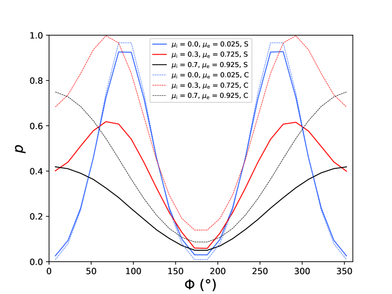
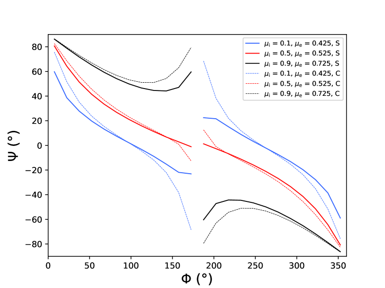
Figure 2.4: The polarisation degree (left) and the polarisation angle (right) versus azimuthal emission angle for various incident and emission inclination angles in the color code, as computed by TITAN and STOKES (solid lines) and as predicted by the Chandrasekhar’s single-scattering approximation (dashed lines). The polarisation degree results are integrated in 10–100 keV, and computed for unpolarized primary with $\Gamma=2.2$ and $\xi=100\,\,\textrm{erg}\cdot\textrm{cm}\cdot\textrm{s}^{-1}$. The polarisation angle results are computed for unpolarized primary and integrated in $E$, $\Gamma$, $\xi$.

2.2 Thermal emission through a disc’s atmosphere

With TITAN and STOKES (v2.33, updated for external undirectional black-body irradiation) we performed numerous simulations for isotropic illumination of a single-temperature unpolarized black-body photon distribution (1.11), passing through a passive constant-density slab. The computational setup is essentially the same as in the previous section, although here we are interested in transmitted spectropolarimetric result. If a constant-density assumption is used, we may operate with the ionization parameter (1.18), which here in combination with bolometric integration of (1.11) (the Stefan-Boltzman law, Stefan, 1879; Boltzmann, 1884) gives

$$\xi_{\textrm{BB}}=\frac{4\pi\sigma T_{\textrm{BB}}^{4}}{n_{\textrm{H}}}\ ,$$ (2.1)

where $\sigma=(2\pi^{5}k_{\textrm{B}}^{4})/(15h_{\textrm{P}}^{3}c^{2})$ is the Stefan-Boltzman constant. This means that we use the natural normalization of the black body, as if the slab was glued directly to the source of this flux, which is convenient when thinking of the case of a colder photosphere directly on top of hotter dissipative disc layers. But in a few illustrative cases below we will also study the effects of a faraway reprocessing slab, e.g. a wind layer distant to a central thermally radiating accretion disc, which would have the flux normalization (and thus $\xi$) reduced by a factor of squared distance to the source. Standard discs should be thermally radiating in the X-rays, if very hot, i.e. requiring a stellar-mass black hole and high mean densities (see Section 1.4). So the main application will be the thermal emission from accretion discs of XRBs. We again neglect Compton up-scattering, which should be effective near the IXPE band at higher slab temperatures than those considered (Prince, 2004), but a quantitative estimate on this assumption could be done with the latest version of STOKES v2.34. On the other hand Compton down-scatterings are important, as the main source of polarisation for individual photons, alongside absorption that effectively reduces the geometry of scattering and adds polarisation. The solar abundance is from Asplund et al. (2005) with $A_{\textrm{Fe}}=1$.

Essentials of this method were published in Taverna et al. (2021) with the code CLOUDY instead of TITAN for disc structure precomputations: locally and then with relativistic integration across the disc. However, the recent advances in X-ray polarimetric observations of XRBs in the thermal state (see Section 5) required a more detailed theoretical exploration of the parametric space than in Taverna et al. (2021), especially in the local frame of reference. In Taverna et al. (2021), the slab was treated in collisional ionization equilibrium (CIE), assuming collisions are the most important process of ionization in dense discs, but a photon ionization equilibrium (PIE) is an equally (un)justifiable assumption for first-order investigations. Although TITAN cannot cover CIE, it is an ideal photoionization code to cross-validate the results of CLOUDY in PIE and, unlike CLOUDY, it offers a) a possibility of double illumination of the slab, which we would use in the future for a combined problem (power-law reflection and black-body transmission self-consistently), and b) a more realistic boundary condition option for optically thick regimes (see below), which we would use in the future for semi-infinite atmospheres with internal source distribution (i.e. towards a more physical atmosphere). Therefore, having the procedures tested in reflection problem already, we explored the local transmission also with TITAN and STOKES in PIE, which is presented here.

Additional local computations in both CIE and PIE, as a follow-up to Taverna et al. (2021), were done simultaneously with CLOUDY and STOKES by Lorenzo Marra. The main principle difference is the inclusion of CIE possibility in CLOUDY as opposed to TITAN, and then obviously the codes’ architecture and individual atomic data inclusion. Although a thorough comparison between TITAN and CLOUDY of the temperature and ionization profiles and spectra, depending on the slab density, irradiation properties and boundary conditions, still needs to be done, we obtained similar results in similar PIE conditions. Thus, not surprisingly, almost identical spectropolarimetric results with STOKES.

This last step, however, confirms correct implementation of the ionization structure input to STOKES from both CLOUDY and TITAN, which was done independently and which is technically not easy, as both photoionization codes provide diverse output information in intricate formats. The new computations with CLOUDY and STOKES in CIE and PIE will not be shown, as they were done and privately communicated by Lorenzo Marra and because a detailed peer-reviewed comparative study is still awaited. More work is also needed to be able to present our results with TITAN and STOKES as a complete parametric grid explored and fully transformed to tabular format for relativistic integration and fitting of any X-ray source, similarly to the reflection tables discussed in the previous section. Hence, we will only show the intermediate discoveries, which lead to tabular summary of only a small (highly ionized) part of the irregular parameter space explored that was immediately used for relativistic integration and direct interpretation of the IXPE observations of 4U1630-47 and LMC X-3 (see Section 5). All of this, including the local atmospheric modeling presented here, was summarized and published in Ratheesh et al. (2024) and Svoboda et al. (2024).

2.2.1 Effects of absorption

First, let us define the problem in terms of optical thickness. An atmosphere of the Novikov-Thorne disc solution is considered optically thick. One can imagine a nearly thermal equilibrium reached by viscous dissipation in deep layers of the disc, which then radiates as a black body and is transformed through colder layers up to some imaginary surface boundary (a density decrease below some negligible value), similarly to radiative transfer inside outer layers of stars.

TITAN offers two types of boundary conditions for PIE with external black-body illumination and a slab with constant density $n_{\textrm{H}}$ and geometrical thickness $H$. One option (irent $=4$) keeps the same effective temperature as the temperature $T_{\textrm{BB}}$ of the single-color black body, i.e. no matter the slab thickness, the temperature profile is roughly the same with monotonically increasing temperature $T$ with Thomson optical depth $\tau_{\textrm{T}}=n_{\textrm{H}}H\sigma_{\textrm{T}}$, where $T(\tau_{\textrm{T}}=1)=T_{\textrm{eff}}\approx T_{\textrm{BB}}$. The other option (irent $=1$) keeps the same temperature at the bottom (illuminated) surface of the slab as the prescribed $T_{\textrm{BB}}$, meaning $T(\tau_{\textrm{T}}=\tau_{\textrm{T,max}}=n_{\textrm{H}}H\sigma_{\textrm{T}}=N_{\textrm{H}}\sigma_{\textrm{T}})\approx T_{\textrm{BB}}$. The two available boundary conditions produce equal results for $\tau_{\textrm{T,max}}\approx 1$. It is the latter case, which is less physical, but used below, because it is identical to CLOUDY treatment of PIE and still valid in optically thin approximation of the upper atmospheric layers playing the largest role in altering the polarisation state of escaping radiation.

In any more sophisticated approach in the future, we would use the first option to assess the entire semi-infinite atmosphere, but that would require also inclusion of internal sources in STOKES (to keep the consistency between ionization structure precomputation and MC spectropolarimetric simulation, using a source function $\tilde{S}$), which we do not have in the presented approach. Inside the slab scattering region, the external black-body photons are only scattered, absorbed and immediately reemitted or absorbed, but not thermalized with radiation and kinetic consequences, which the MC method cannot process. Also, in case of a more realistic semi-infinite atmosphere a hydrostatic equilibrium would have to be used.

The ignored phenomena were essentially included and altogether studied simultanously to our efforts by Valery Suleimanov using spectropolarimetric radiative transfer solver, adapted from Suleimanov et al. (2002, 2007). This model, including relativistic disc integration, was part of the data interpretation of IXPE observation of 4U1630-47 and it is also summarized in Ratheesh et al. (2024) (see in particular figure B1 for local emission at two different rings and figure B2 for the net result with and without the relativistic effects). Even more physical computation, taking into account density inhomogeneities (Coleman and Shields, 1990) and magnetic force support was done by Davis et al. (2009), using MHD approach combined with 3D MC simulation for emergent polarisation.

Self-consistent models of a semi-infinite local disc atmosphere serve as a good cross-validation to our simplified approach, but inevitably contain many internal parameters and are computationally costly, which makes them less flexible for data fitting. Our Milne approach with a passive slab sitting on external black-body source is less robust, but if proven to provide reasonably similar spectropolarimetric results with inclination, density and effective temperature, it introduces only the problem of height scaling and ionization structure, which shall be fine-tuned to represent the effects of a real photospheric transition medium between the matter in thermal equilibrium at high temperatures in the midplane and nearly vacuum on the other side. If the free parameter of our finite-slab model, the optical depth $\tau_{\textrm{T,max}}$, is too large, we depart from a more physical situation by neglecting internal sources of thermal radiation inside the slab. If it is too low, we may underestimate the absorption and scattering effects. As we will show below, in comparison with X-ray spectroscopic and energy-dependent polarisation data, we will validate and use our model for fitting in only part of the thinkable parameter space. The rest of the computations, perhaps too artificial, only help to understand the role of elementary processes in the emergent polarisation.

Apart from range of optical depths, we also tested several orders of magnitude in $n_{\textrm{H}}$, because a physical atmosphere would have a dominantly decreasing density profile with vertical height (e.g. a gaussian profile, or more general ones are derived, Shakura and Sunyaev, 1973; Davis et al., 2006; Taverna et al., 2020). This was done also in order to test possible application of the model, assuming radial disc integration and various radial disc density profiles, $n_{\textrm{H}}(r)$, alongside various effective temperature profiles, $T_{\textrm{eff}}(r)$, that can appear according to the Novikov-Thorne estimates. After several simulation trials we proved that in the PIE conditions studied ($n_{\textrm{H}}=10^{12}$–$10^{20.5}\ \textrm{cm}^{-3}$, $k_{\textrm{B}}T_{\textrm{BB}}=0.16$–$1.4\ \textrm{keV}$, $\tau_{\textrm{T,max}}\geq 0.4$, $\xi=\xi_{\textrm{BB}}$) a) the resulting polarisation angle is always constant with energy and parallel with the slab (as expected for a passive atmosphere with scattering and absorption and moderate or high optical thickness) and b) the shape of the resulting polarisation degree with energy is heavily dependent on ionization structure (in turn dependent on $n_{\textrm{H}}$, $T_{\textrm{BB}}$ and $\tau_{\textrm{T,max}}$) – no matter how the ionization state of the slab is prepared – and then scaled at all energies uniformly with $\mu_{\textrm{e}}$ and $\tau_{\textrm{T,max}}$.

We will explain the results in depth in terms of absorption and scattering effects below, but in order to separate the effect of varying ionization with $\tau_{\textrm{T,max}}$ from the effects of pure $\tau_{\textrm{T,max}}$ on the emergent polarisation in the resulting figures, we made an additional modeling choice based on the preliminary parametric behavior. We decided to fix the ionization profile precomputed with TITAN at $\tau_{\textrm{T,max,structure}}=1$ and then rescale this ionization structure when computing with STOKES by extending or shrinking the height of the entire slab $H$, reaching different $\tau_{\textrm{T,max}}$ for the same ionization profile. This goes certainly against the original idea of keeping the two computational phases and their setups as equal as possible, but it is a reasonable trade-off for understanding of what causes what inside the slab. Nonetheless, for any thicker slabs we would not be able to keep the STOKES setup identical to the ionization structure precomputations due to lack of internal thermal sources and the constant-temperature boundary condition becomes invalid for a realistic ionization structure estimate. For data fitting later on, we will use only the highly ionized results where caveats with respect to partial ionization do not apply. In the partially ionized cases, if shrinking or extending vertically stratified ionization profile obtained with TITAN for $\tau_{\textrm{T,max,structure}}=1$, we overestimate or underestimate the real consistent ionization gradient for final thickness $\tau_{\textrm{T,max}}$, respectively.

We first assumed a stratification of 500 layers in TITAN and then again averaging to up to 50 layers in STOKES during the conversion of the ionization structure information. After comparing the results for $\tau_{\textrm{T,max,structure}}=1$ with just averaging to 1 layer in STOKES as the entire slab, there was negligible difference in the spectropolarimetric results and the temperature and ionization stratification obtained in TITAN was low. Therefore, we continued with single-layer approximation for computational efficiency in the MC simulation for all results presented below.

Having laid down the procedure and giving away the main features, let us study the effects of partial ionization in detail. Figures 2.5 and 2.6 show the effects of changing density for particular single-temperature black-body illumination with $\xi=\xi_{\textrm{BB}}$ and $k_{\textrm{B}}T_{\textrm{BB}}=0.16$ keV. We show the fractional abundances of iron and oxygen ions from TITAN (taken at intermediate layer with temperature closest to the averaged layer in STOKES) to show that the lower the density, the higher the ionization. For the highly ionized cases, the atomic nuclei are nearly stripped off all electrons. Next, we show the effective optical depth (Rybicki and Lightman, 1979)

$$\tau_{\mathrm{eff}}=\sqrt{3\tau_{\mathrm{abs}}(\tau_{\mathrm{abs}}+\tau_{\mathrm{es}})}\ ,$$ (2.2)

where $\tau_{\mathrm{abs}}$ is the total (sum of bound-free and free-free) absorption optical depth and $\tau_{\mathrm{es}}$ is the electron scattering optical depth, which is the best information we can obtain on continuum opacities from TITAN, including the provided line optical depths, which are plotted on top of the continuum. We divide by the total column density $N_{\textrm{H}}$ to compare to energy-independent Thomson cross section $\sigma_{\textrm{T}}$ for pure scattering in elastic limit. Although this comparison is not very clarifying due to mixture of competing effects forming the effective optical depth, within the peculiarities of TITAN outputs it gives the only available estimate on absorption importance (including ionization edges) and scattering. We then provide the corresponding density examples of the STOKES output spectra for $\tau_{\textrm{T,max}}=1$ and a series of corresponding polarisation fractions with energy from STOKES for the same densities and for $\tau_{\textrm{T,max}}=\{0.67,1,3\}$.

Figure 2.5: Various cases of transmitted single-temperature unpolarized black-body radiation with $k_{\textrm{B}}T_{\textrm{BB}}=0.16$ keV through a constant density slab, as computed with TITAN and STOKES in PIE. From left to right the density of the slab decreases ($n_{\textrm{H}}=10^{18},10^{17},10^{16},10^{15},10^{14}\ \textrm{cm}^{-3}$, respectively) and the slab is more ionized for the same external illumination with $\xi=\xi_{\textrm{BB}}$. Top row: fractional abundance of ions of oxygen (blue) OI–OIX and iron (red) FeI–FeXXVII from TITAN ionization structure precomputations. Middle row: the effective optical depth, $\tau_{\textrm{eff}}$, divided by column density, $N_{\textrm{H}}\,[\textrm{cm}^{-2}]$, versus energy for continuum processes (black) and including lines (cyan) from TITAN ionization structure precomputations. Thomson cross-section $\sigma_{\textrm{T}}$ (yellow) represents pure scatterings. Bottom row: spectra, $F$, per energy bin for various observer’s inclinations $\theta$ in the color code for $\tau_{\textrm{T,max}}=1$, obtained from STOKES.

Figure 2.6: The polarisation degree, $p$, versus energy obtained from STOKES (solid lines) for various observer’s inclinations $\theta$ in the color code, corresponding to the cases shown in Figure 2.5. From left to right the density of the slab decreases ($n_{\textrm{H}}=10^{18},10^{17},10^{16},10^{15},10^{14}\ \textrm{cm}^{-3}$, respectively) and the slab is more ionized for the same external illumination. Top row: the results for $\tau_{\textrm{T,max}}=0.67$. Middle row: the results for $\tau_{\textrm{T,max}}=1$ (corresponding directly to the spectra shown in bottom pannels of Figure 2.5). Bottom row: the results for $\tau_{\textrm{T,max}}=3$. We indicate the pure-scattering limit for semi-infinite atmosphere given by Chandrasekhar-Sobolev approximation for the same inclination values (dashed horizontal lines). The obtained polarisation angle from STOKES is constant with energy and parallel with the slab.

At energies where the spectra are heavily absorbed, the polarisation degree rises steeply. If the photo-electric opacity is higher at a particular energy band, it induces polarisation through absorption combined with the underlying black-body distribution. An inclined observer sees photons that are arriving in vertical directions to the escaping surface region with more probability than photons that would travel diagonally through the slab without being absorbed. Hence, the geometry is effectively reduced and the observer sees polarized photons roughly according to (1.17). For this reason, absorption raises polarisation with increasing slab thickness $\tau_{\textrm{T,max}}$ and for a given thickness with $\theta$ at all energies. It is just that at particular energies, the absorbtion effects may be more significant relative to elsewhere and the general presence of absorption effects is linked to the ionization state. The cases with high or moderate absorption reproduce the results in Taverna et al. (2021) (see e.g. figure 3 or 8), the spectra are highly absorbed mostly around 3 keV and polarisation rather decreases with energy at 2–8 keV, because of the high gain of polarisation around 3 keV. If the density is low enough, so that the slab is almost fully ionized, the polarisation is steady or increases with energy at 2–8 keV, as at about 3 keV there is small absorption left and only the peak at about 10 keV remains in the broadband view. This peak is caused by absorption on top of scattering due to remaining ionization edges, particularly an iron edge at 9 keV, and due to Compton down-scattering effects. The latter causes higher polarisation of emergent photons at higher energies that scattered fewer times with respect to those emergent at lower energies, similarly to the effects in reflection described in Section 2.1.1. The state of complete ionization that would result in pure-scattering results and energy-independent polarisation degree for elastic scattering at $E\lessapprox 2$ keV and with even lower 2–8 keV average value, could not be reached in the studied conditions with the radiative transfer codes, if not ad hoc forced to neglect the absorption effects.

Although absorption in this model scenario can in principle raise polarisation to ever increasing polarisation, as the inclination dependent single-scattering limit (1.17) allows, scattering-induced polarisation has a finite polarisation limit given by the Chandrasekhar-Sobolev result for semi-infinite atmosphere in Thomson regime, approximated by (1.40). This limit is also inclination dependent and drawn in dashed lines in Figure 2.6. In Taverna et al. (2021), it was proved that in pure-scattering regime the CLOUDY and STOKES simulations reach Chandrasekhar’s limit for $\tau_{\textrm{T,max}}\gtrapprox 3$ for low enough energies (to ignore the down-scattering effects at higher energies). In our results that include absorption and Compton down-scattering, we typically observe a plateau in polarisation in between 0.2–1 keV that for $\tau_{\textrm{T,max}}\gtrapprox 3$ also precisely reaches the Chandrasekhar’s value. Therefore, at these energies we are at the pure-scattering Thomson regime with negligible absorption contribution. Elsewhere polarisation at high $\tau_{\textrm{T,max}}$ can exceed this limit, as absorption is added on top of the scattering results, because additional anisotropy in photon directions inside the medium is enforced and down-scattering energy redistribution effects on polarisation are scaled too. The $\tau_{\textrm{T,max}}$ parameter does not have any theoretical constraint, because it serves as a free parameter of our model, which can approximate a more complex model or real observation with any value between zero and infinity. The effects of incident changing black-body temperature on the emergent polarisation will be discussed in the next section.

If density is monotonically increased, the spectra are first heavily absorbed at around 3 keV, which causes the additional increase of polarisation, forming a large polarisation peak at 2–6 keV. The same patterns in spectra and polarisation with high absorption added by density occurs for higher $T_{\textrm{BB}}$, but generally higher densities are needed to absorb X-ray illumination with higher $T_{\textrm{BB}}$ [see (2.1)]. As soon as a particular high ionization threshold is reached by decreasing density (right side of the figures), the results of the simulation look identical for ever decreasing density and a state of full ionization cannot be reached in the numerical simulations. This could also justify the constant-density assumption in such highly ionized limit, apart from comparisons to hydrostatic-equilibrium models. It is important to note that high ionization ($\xi_{\textrm{BB}}\gtrapprox 10^{5}\,\textrm{erg}\cdot\textrm{cm}\cdot\textrm{s}^{-1}$) is actually the most natural state of such slabs in PIE under these conditions. For illumination with temperature as low as $k_{\textrm{B}}T_{\textrm{BB}}=0.5$ keV (for e.g. 4U1630-47 the mean was $k_{\textrm{B}}T_{\textrm{BB}}\approx 1.15$ keV, Ratheesh et al., 2024), we already require $n_{\textrm{H}}\gtrapprox 10^{20.5}\ \textrm{cm}^{-3}$ to see the strong absorption features near 3 keV. Such extreme astrophysical densities are already beyond the convergence limits and trustworthy computations with TITAN and the atomic data used, as well as they are difficult to be believed to exist in upper layers of the XRB disc atmospheres, although sometimes considered in literature (see e.g. Liu et al., 2023). Moreover, XRB sources like 4U1630-47 or LMC X-3 that we will focus on in Section 5 do not show significant (orders-of-magnitude) flux absorption in the soft state, they are rather highly ionized with thermal peak well representing a multi-temperature black-body curve with a few ionization edges and spectral lines.

We also tested that similar absorption behavior occurs by keeping the slab density fixed and decreasing the ionization parameter by decreasing flux normalization, i.e. as if the slab was a wind layer placed further and further from a diffuse thermally radiating body. The results are shown in Figures A.2 and A.3 in Appendix A. Again, even for a few orders of magnitude lower $\xi$ than $\xi_{\textrm{BB}}\approx 2.3\times 10^{7}\,\textrm{erg}\cdot\textrm{cm}\cdot\textrm{s}^{-1}$ for this case, we are in the highly ionized limit where all spectropolarimetric results are identical up to some numerical noise. The fact that polarisation is ionization dependent, but it does not matter in what conditions the gas achieved such ionization state, makes it difficult to disentangle the origin(s) of emission and geometry of the studied medium within the inner-accreting system, if spectroscopy of both continuum and lines also shows degeneracies in this manner. A reduction of complete photon isotropy of the source of radiation would affect polarisation for lower optical depths.

The same dependency on absorption with identical spectropolarimetric features was found by Lorenzo Marra in various regimes of PIE with CLOUDY, as well as in CIE with CLOUDY, if orders of magnitude higher slab temperatures ($T_{\textrm{slab}}\gtrapprox 10^{8}\,K$) were assumed than in the CIE examined in Taverna et al. (2021). Therefore, with these recent advances altogether, we enlarged the still narrow view of the problem that was provided in Taverna et al. (2020) not only in energy range, but in the ionization level. We showed how (with energy and amplitude) the absorption effects disappear and that there is some sort of saturation for high enough ionization, but not full ionization, as we still see some absorption effects mostly due to a remaining iron edge. The temperatures required to reach such high ionization limit in CIE would lead to strongly inverted temperature profiles with the top of the atmosphere being hotter than the emitting layer of the disc, which is not expected for realistic atmospheres (Davis et al., 2005; Różańska et al., 2011). Thus, if high ionization is required, CIE is perhaps a less viable model than PIE, which produces a monotonically decreasing temperature profile counted from the side of external illumination.

2.2.2 The limit of high ionization

Because the absorbed cases produce polarisation profiles with energy that are highly degenerate with other parameters in play and because we argued that we do not model properly thick and absorbing slabs, we will now focus only on the highly ionized results. Not only that high ionization is expected, especially in inner parts of the disc, which tend to have higher contribution to the total flux after relativistic integration (see e.g. Dovčiak et al., 2004b), they are more supported by the first IXPE results for XRBs in the soft state that tend to show increasing polarisation degree with energy in 2–8 keV (see Section 5). We will argue later that relativistic effects for a standard disc integration in summed polarisation tend to rather depolarize at higher energies and we have argued already that any increase of absorption due to $n_{\textrm{H}}$ change or $\xi$ change starts raising the polarisation first near 3 keV, causing at parts or in the whole 2–8 keV range locally a steady or decreasing polarisation with energy. Hence, an efficient mechanism for production of polarisation rising with energy is required, which the highly ionized slab may offer.

In the high ionization limit, black-body temperature forms the underlying photon distribution, but the ionization structure is temperature and density independent, which is ideal for constructing radial profiles of emission that strongly depend on effective temperature and density in the Novikov-Thorne model. This would not be the case for absorbed polarisation profiles, as in Figure 2.6, where the $\xi(T_{\textrm{BB}},n_{\textrm{H}})$ fine-tuning of ionization in the local comoving frame with the disc would have to match in the net result for a particular disc temperature and density radial profile, including polarisation modification due to GR effects.

Figures 2.7 and 2.8 show again for a few selected temperatures and high densities (within the high ionization saturation of polarisation profiles): the ionization levels, continuum and line optical depths, spectra from STOKES (only for $\tau_{\textrm{T,max}}=1$), and the resulting polarisation degree with energy. We refer to the detailed study of Davis et al. (2005, see their figures 1 and 4) for estimates on energy-dependent contributions of various processes to the total opacity of XRB local disc emission. Photoelectric absorption cross-section generally declines as $\sim E^{-3}$ and is already less important compared to scattering above $\approx 0.2$ keV (compare the $\tau_{\textrm{eff}}/N_{\textrm{H}}$ values with $\sigma_{\textrm{T}}$ with polarisation shape with energy around 0.1 keV). The scattering cross-section is constant up to $\approx 0.5$ MeV, below which $\sigma_{\textrm{KN}}\approx\sigma_{\textrm{T}}$. However, in the IXPE energy range, this trend of scattering importance relatively to absorption is reversed due to the presence of a strong iron ionization edge at 9 keV, even for the highly ionized slabs. It causes the aforementioned stronger polarisation than the pure-scattering limit at about 10 keV, which is also convolved with the underlying black-body photon distribution, as down-scattering effect on polarisation is in play. This remaining peak in polarisation is then shifted in energy, as the underlying black-body peak is shifted. The polarisation peak is flattened towards higher energies, but we observe the black-body distribution effects combined with the remaining sharp ionization edge at 9 keV.

We can conclude in the following way. High absorption and Compton down-scattering effects (as opposed to the Thomson elastic limit) along with high inclination generally results in high average polarisation degree, increasing with energy in 2–8 keV. The slope of polarisation with energy in 2–8 keV is given by $\tau_{\textrm{T,max}}$ and $\mu_{\textrm{e}}$ and to a lesser extent by $T_{\textrm{BB}}$. For highly ionized sources with high enough mean temperatures, the pure-scattering Thomson plateau at soft X-rays reaches 2 keV. At 2 keV, we are thus closer to pure Thomson scattering than at the upper part of the IXPE range. If Compton up-scattering effects were considered in the simulation, they would presumably act against the down-scattering energy redistribution of photons, thus lifting this energy threshold where polarisation matches the Thomson scattering results to higher energies. This remains to be quantitatively tested with the latest version of STOKES v2.34.

Hence, the value of polarisation fraction at 2 keV in some spectral states can constrain the lower limit on inclination according to (1.40) in optically thick regime (any higher inclination value can be achieved with finite $\tau$, which is an ad hoc parameter of our model) with some assumption on observed geometry. The IXPE observed slope of polarisation degree with energy at 2–8 keV can in addition serve as a first-order estimation tool for inclination, knowing the neglect of local up-scattering and relativistic integration effects.

Typically, if considering a photosphere located on top of equatorial inner disc, a subsequent relativistic integration would result in depolarisation; hence, requiring even higher local slab inclinations with respect to the observed polarisation at 2 keV when compared with non-relativistic models. Near black hole, the local emission angle with respect to normal is rather decreased due to strong-gravity effects, plus more trajectories with various polarisation angles are combined in GR (Dovčiak et al., 2004b).

Figure 2.7: Various highly ionized cases of transmitted single-temperature unpolarized black-body radiation through a constant density slab, as computed with TITAN and STOKES in PIE. From left to right the temperature of the illuminating black body increases ($k_{\textrm{B}}T_{\textrm{BB}}=0.23,0.50,0.80,1.15,1.40$ keV, respectively), while the densities are high ($n_{\textrm{H}}=10^{15},10^{20},10^{20.5},10^{20.5},10^{20.5}\ \textrm{cm}^{-3}$, respectively), but not high enough to depart from the saturation state and to cause significant absorption for a given $\xi=\xi_{\textrm{BB}}$. For any lower density we would see identical result. Top row: fractional abundance of ions of oxygen (blue) OI–OIX and iron (red) FeI–FeXXVII from TITAN ionization structure precomputations. Middle row: the effective optical depth, $\tau_{\textrm{eff}}$, divided by column density, $N_{\textrm{H}}\,[\textrm{cm}^{-2}]$, versus energy for continuum processes (black) and including lines (cyan) from TITAN ionization structure precomputations. Thomson cross-section $\sigma_{\textrm{T}}$ (yellow) represents pure scatterings. Bottom row: spectra, $F$, per energy bin for various observer’s inclinations $\theta$ in the color code for $\tau_{\textrm{T,max}}=1$, obtained from STOKES.

Figure 2.8: The polarisation degree, $p$, versus energy obtained from STOKES (solid lines) for various observer’s inclinations $\theta$ in the color code, corresponding to the cases shown in Figure 2.7. From left to right the temperature of the illuminating black body increases ($k_{\textrm{B}}T_{\textrm{BB}}=0.23,0.50,0.80,1.15,1.40$ keV, respectively), while the densities are high ($n_{\textrm{H}}=10^{15},10^{20},10^{20.5},10^{20.5},10^{20.5}\ \textrm{cm}^{-3}$, respectively), but not high enough to depart from the saturation state and to cause significant absorption for a given $\xi=\xi_{\textrm{BB}}$. For any lower density we would see identical result. Top row: the results for $\tau_{\textrm{T,max}}=0.67$. Middle row: the results for $\tau_{\textrm{T,max}}=1$ (corresponding directly to the spectra shown in bottom pannels of Figure 2.7). Bottom row: the results for $\tau_{\textrm{T,max}}=3$. We indicate the pure-scattering limit for semi-infinite atmosphere given by Chandrasekhar-Sobolev approximation for the same inclination values (dashed horizontal lines). The obtained polarisation angle from STOKES is constant with energy and parallel with the slab.

We constructed tables in the high ionization limit that allow for disc integration and more valuable fitting than directly in the local comoving frame, using the relativistic KY codes. The density independence of the highly ionized slab results allowed us to select one density $n_{\textrm{H}}=10^{18}\ \textrm{cm}^{-3}$ and compute a grid of polarisation fractions with energy in the 1–20 keV range that is dependent only on $\mu_{\textrm{e}}=\{0.025,0.075,...,0.925,0.975\}$, $k_{\textrm{B}}T_{\textrm{BB}}=\{0.5,0.8,1.15,1.4\}$ keV and the critical free parameter $\tau_{\textrm{T,max}}=\{0.2,0.4,0.67,1,1.3,1.5,2,3,5,7,10\}$ that controls the level of absorption and down-scattering effects on polarisation by scaling the slab height, but not to the detriment of ionization level, which is fixed. We manually checked that no strong absorption features near 3 keV emerged for the selected choice of values, i.e. that we stay in the desired highly ionized limit (for $\xi=\xi_{\textrm{BB}}$) and that all has converged (an MC effect of artificially high polarisation for low photon statistics was found). Because some stochastic numerical noise is unavoidable (but not artificially high polarisation due to very low computational times) and because any disc integrator would appreciate to interpolate smooth functions, we opted for smoothing the results by performing linear regression of the model curves for two polynomials of third order ($y=A^{\prime}x^{3}+B^{\prime}x^{2}+C^{\prime}x+D^{\prime}$), one applied below the 9 keV edge at 1–9 keV, and the other at 9–20 keV. Hence eight coefficients were provided for the parameter space here above, which are meant to be implemented to relativistic integrators for fast data fitting of highly ionized sources. The 1–20 keV total energy range was chosen, because of anticipated relativistic energy shifts of photons further out from the 2–8 keV IXPE band.

Last but not least, we ought to check in which conditions this fitting model is not valid anymore. One should worry any time when the fits are ending in corners of the parameter space. Here particularly low $T_{\textrm{BB}}$ and high $\tau_{\textrm{T,max}}$ could mean a departure from the highly ionized state. Because repeatedly high $\tau_{\textrm{T,max}}$ were needed to explain the IXPE data (see Section 5), an interesting theoretical question emerged whether for ever increasing $\tau_{\textrm{T,max}}$ by changing height of the layer (and keeping the high ionization level) we would get some saturation in the increasing polarisation, or how to extrapolate the MC results for higher $\tau_{\textrm{T,max}}$. Although numerous nights were spent on this problem with blurry conclusions and a numerical experiment would require years on available institutional computational clusters, it was eventually abandoned even as a toy-model explanation of extreme polarisation increasing with energy, because of the necessity of loosing the required ionization levels on the further (not illuminated) side of the slab for thick slabs that would lead to additional absorption features near 3 keV (see Figures 2.5 and 2.6). Also because of the neglect of internal sources in such model that would on the contrary depolarize the net output, providing sources of radiation with lower distance to the surface than the external source. We checked with additional vertically stratified calculations that given the lowest temperatures and highest densities, the further side of the slab looses the required level of ionization at $\tau_{\textrm{T,max}}\gtrapprox 10$ and the models should generally not be used beyond this value. Higher $\tau_{\textrm{T,max}}$ may be in some cases explored, but the limits of validity are density and temperature dependent.

The sensitivity of the results to the assumption of no internal sources can be evaluated by comparison with the model of Valery Suleimanov in Ratheesh et al. (2024), which shows great similarities with the provided results for local emission of highly ionized disc rings (figure B1, bottom left panel, Ratheesh et al., 2024), despite using a completely different radiative transfer method. The same energy-independent plateau in polarisation that we obtained below 2 keV is formed. And equally to our model, the polarisation dependence on inclination in this range follows exactly the pure-scattering law (1.40). The dependency of polarisation on ionization edge is more pronounced compared to our case and the energy-independent plateau is extended up to 9 keV, where a sharp increase in polarisation occurs due to the remaining iron edge. The result is then substantially different compared to ours for the outer disc rings (figure B1, bottom right panel, Ratheesh et al., 2024), where the highly ionized limit is not valid anymore. The non-relativistic integration of this model (figure B2, dotted lines, Ratheesh et al., 2024) preserves the pure-scattering result at soft (0.1–1 keV) and mid (1–10 keV) X-rays, suggesting higher weighting of the highly ionized disc rings.

Note that the relativistic integration (figure B2, solid lines, Ratheesh et al., 2024), apart from depolarisation with slight energy dependence, alters the energy dependence of the resulting polarisation angle. In Section 5 we will show results where our local model was relativistically integrated, taking this effect into account too for data fitting of the observed polarisation angle with energy.

One may also compare our results to the sophisticated MHD simulations done by Davis et al. (2009, figures 7–9, 12, 15), which include the effects of magnetic fields with carefully computed effects of Faraday rotation and inhomogeneities on the net X-ray polarisation. The predicted polarisation is parallel to the disc and constant according to the Chandrasekhar-Sobolev profile in between 0.2–4 keV without the affects of Faraday rotation. The Faraday rotation in addition depolarizes the signal and causes increasing polarisation with energy at soft X-rays and non-trivial polarisation orientation, in accordance with earlier study of Gnedin et al. (2006). These works are departing from earlier estimates by Gnedin and Silant’ev (1978); Silant’ev (1979); Laor et al. (1990); Agol and Blaes (1996); Blaes and Agol (1996); Agol et al. (1998); Agol and Krolik (2000).

2.2.3 Summary

Let us provide a quick summary of the above. Using a combined radiative transfer and MC method, we constructed simulations of a passive plane-parallel slab of constant density that alters the polarisation state of the unpolarized illuminating isotropic single-temperature black-body source of radiation, located from the opposite side of the slab with respect to a generally inclined observer. The slab was held in PIE (a few comparisons with CIE approach showed similar results, but for higher temperatures needed inside the simulated top atmospheric layers) and the obtained vertical stratification was in general negligible for moderate optical depths. If the illuminating flux is low, or the density or optical depth is high, the polarisation may be on average high (even tens of %) in 2–8 keV, decreasing with energy due to a strong peak at 3 keV. This peak gradually disappears by e.g. lowering the slab density and a certain polarisation degree profile with energy establishes for high enough ionization (a state of full ionization could not be reached in the studied PIE conditions) with lower polarisation in 2–8 keV and with a steady or increasing polarisation degree with energy. As long as the slab optical thickness is higher than $\tau_{\textrm{T,max}}\gtrapprox 0.4$, the resulting polarisation angle is constant with energy and parallel with the slab. The polarisation degree in the highly ionized regime reaches Thomson scattering values at 2 keV given by the Chandrasekhar-Sobolev analytical results, if $\tau_{\textrm{T,max}}\gtrapprox 3$. The model should not be used above $\tau_{\textrm{T,max}}\gtrapprox 10$, as beyond we depart from the high level of ionization in the PIE conditions studied. In general, the simulation is a toy model (introducing a free parameter of $\tau_{\textrm{T,max}}$ of the passive slab) of a real atmosphere on top of hot dissipative layers closer to the disc mid-plane. A more realistic models for comparison include internal sources of radiation, compute the entire semi-infinite problem (assuming e.g. a hydrostatic equilibrium) and include the effects of magnetic fields. However, due to simplicity, our model is suitable for first-order estimates on e.g. inclination, if compared with IXPE observations of XRBs with highly ionized thermally dominated spectra, especially if relativistically integrated across a disc with assumed geometry and temperature profile. This was facilitated by tabulating a smoothed function of the polarisation state with energy in 1–20 keV for a relevant part of the explored parameter space, dependent only on inclination, optical depth and local effective temperature.

Chapter 3 Total emission from an inner-accreting region

In this chapter, we characterize emission from the entire inner disc-corona system in the lamp-post geometry and compare it to a toy model simulating a sandwich geometry. We present the local reflection tables that were described in Section 2.1, integrated across the disc for a distant observer. All relativistic effects are included, apart from returning radiation after the first reflection from the disc. The first reflection is accounted for and it will be of our prime interest. For these computations, a new KY routine, called KYNSTOKES, was developed, based on the radiative transfer kernels of the previously published KY codes. Thermal disc radiation is not included; hence, the results (also with respect to the assumed densities) are rather applicable as toy models of inner-accreting regions of AGNs than XRBs.

Essentials of the KYNSTOKES lamp-post model with implementation of the TITAN and STOKES local reflection tables were developed and described in Podgorný (2020), which we will only briefly summarize. Over the scope of this dissertation, KYNSTOKES in the lamp-post regime was tested and the results were discussed in more depth and context, as published in Podgorný et al. (2023a), but with the previous version of reflection tables from Podgorný et al. (2022). Here we will list the findings from Podgorný et al. (2023a) and plot the corresponding and additional figures with an updated KYNSTOKES routine, interpolating in the local reflection tables unified in $\xi$ that were described in Section 2.1.

In addition, the slab coronal model was implemented to KYNSTOKES based on earlier work of Michal Dovčiak and the results were discussed with respect to the lamp-post model in KYNSTOKES over the scope of this dissertation. We provide the related key points at the end of this chapter, but we note that this part is still awaiting a peer review. The same holds for dependency of the emission on the inner disc radius, which was not covered in Podgorný et al. (2023a) even for the lamp-post model (although the public version of the code allows to truncate the disc) and which we also add here for both studied geometrical archetypes of the corona.

The KYNBBRR routine, suitable for fitting thermal radiation of XRBs, was recently updated thanks to Michal Dovčiak to its KYNEBBRR variant, which implements the local thermal emission from highly ionized disc atmosphere computed with TITAN and STOKES, i.e. the one described at the end of the previous chapter. The relativistically integrated results obtained with this routine will be presented only briefly as part of the observational results in Chapter 5 and not here, because the implementation, testing and discussion was done by colleagues that were involved in Dovčiak et al. (2008); Taverna et al. (2020, 2021); Mikušincová et al. (2023) and that developed the KYNBBRR model.

Aside to the main results obtained with KYNSTOKES, we also propose in Appendix B an alternative way of integrating the disc emission inside the KY codes in general. It would, however, require rewriting large portions of the main scripts to provide thorough testing, or perhaps developing a new code. Because the outcomes in gained efficiency did not seem outstanding on the first sight, we decided not to continue further in this direction. Another reason is that the proposed alternative scenario for disc integration was intended to improve precision in detailed relativistic smearing of e.g. spectral lines, which is beyond the resolution of any current or forthcoming X-ray polarimeter, hence slightly out of the main focus of this dissertation.

3.1 The lamp-post coronal model

A motivation for this study was possible improvement of the model in Dovčiak et al. (2011), which considered the single-scattering Chandrasekhar’s formulae (1.39) for reflection-induced polarisation and the NOAR spectral computations of reflecting neutral accretion disc. The ionization structure of the disc was not considered, nor any spectral lines. Only the unpolarized primary emission was studied in Dovčiak et al. (2011) and although the code was updated for polarisation of the primary radiation for the AGN modeling described in Marin et al. (2018a, b), an error was found by Michal Dovčiak in the GR computations of polarisation angle change used therein. Then, as part of this dissertation, the computations of the change of polarisation angle due to GR effects between the lamp and the disc and between the lamp and the observer, originally performed by Michal Dovčiak, were revisited and verified. This is shown in Appendix C. Independently, we also discovered an error in Dovčiak et al. (2011) in the local reflection prescriptions for polarisation (fixed and described in appendix B of Podgorný et al., 2023a), which propagated into the global computations of both polarisation angle and degree, i.e. figs 6 and 8–14 in Dovčiak et al. (2011). Thus, it is worth to revisit the entire discussion of the lamp-post results for a distant observer that appeared in Dovčiak et al. (2011), instead of doing a one-to-one comparative study that would show only the effects of modeling improvements.

We refer to Figure 1.23a for a sketch of the parametrization and to Sections 1.1.3 and 1.5.2 for the main physical setup of the model. In the plots below, we will assume three cases of disc ionization, given by the luminosity of the primary (increases the local $\xi$) and black-hole mass (scales the distance in physical units between the source and the disc): “low ionization” ($M=1\times 10^{8}\,M_{\odot}$ and the observed 2–10 keV flux $L_{\textrm{X}}/L_{\textrm{Edd}}=0.001$), “moderate ionization” ($M=3\times 10^{6}\,M_{\odot}$ and the observed 2–10 keV flux $L_{\textrm{X}}/L_{\textrm{Edd}}=0.01$), and “high ionization” ($M=1\times 10^{5}\,M_{\odot}$ and the observed 2–10 keV flux $L_{\textrm{X}}/L_{\textrm{Edd}}=0.1$). The disc is assumed to have a constant radial density profile, given by the local reflection tables with $n_{\textrm{H}}=10^{15}\ \textrm{cm}^{-3}$, but in principle the code can scale density radially by means of local ionization parameter change. The disc inner radius $r_{\mathrm{in}}$ is fixed at the ISCO and $r_{\mathrm{out}}=400\,r_{\textrm{g}}$, if not stated otherwise. We will study the case of reflected-only radiation with $N_{\textrm{p}}/N_{\textrm{r}}=0$ and the case of added primary source with $N_{\textrm{p}}/N_{\textrm{r}}=1$, i.e. a consistent one-to-one normalization of the primary and reflection contribution, according to the local reflection tables. The primary source is point-like and isotropic, which is one of the most critical simplifications of this work, as neither the flux nor the polarisation is expected to be isotropic in the lamp-post regime due to Comptonization of disc seed photons (e.g. Zhang et al., 2019b; Krawczynski and Beheshtipour, 2022; Zhang et al., 2022, 2023). The local reflection tables are interpolated per each geodesic in the local reflection angles as well as in the three precomputed polarisation states of primary irradiation. The arbitrary state of primary radiation for the locally emergent Stokes parameters $I$, $Q$ and $U$, commonly denoted as $S$, is obtained through

$$\begin{split}S(p_{0},\Psi_{0}+\Delta\Psi)=&\,S(0,-)+p_{0}\Big{\{}\Big{[}S(1,0)-S(0,-)\Big{]}\cos{2(\Psi_{0}+\Delta\Psi)}\\ &\quad+\left[S\left(1,\frac{\pi}{4}\right)-S(0,-)\right]\sin{2(\Psi_{0}+\Delta\Psi)}\Big{\}}.\end{split}$$ (3.1)

thanks to the linearity of Stokes parameters.

3.1.1 Spectropolarimetric properties

We will first show the results for $\Gamma=2$ and unpolarized primary radiation. The obtained reflected-only and total spectra are shown in Figures 3.1 and 3.2 for two extreme black-hole spins, three inclinations, two lamp-post heights and three cases of disc ionization. The spectra are corrected for slope change and renormalized to value at 50 keV to see the distinct line and continuum features clearly. In all cases, the relativistic smearing occurs, compared to the local reprocessing profile. The relativistic effects are the strongest when most radiation reaches the inner disc (i.e. for low lamp-post heights and high black-hole spin) and for high inclinations. The added primary radiation suppresses the reflection features, and the differences from a plain power-law are minor (the $y$-axis in Figure 3.2 is stretched compared to Figure 3.1). The relativistic routines are well-tested (see e.g. Dovčiak et al., 2004b) and the spectral results resemble other lamp-post reflection models (García et al., 2014).

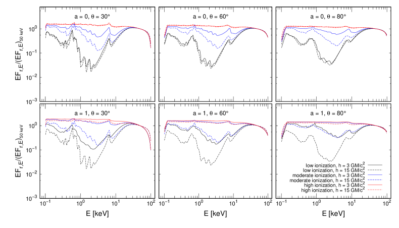
Figure 3.1: The reflected-only spectra of the accretion disc for distant observer, $EF_{\mathrm{r,E}}$, normalized to value at 50 keV, obtained by KYNSTOKES for black-hole spins $a=0$ (top) and $a=1$ (bottom), disc inclinations $\theta=30^{\circ}$ (left), $\theta=60^{\circ}$ (middle) and $\theta=80^{\circ}$ (right), $\Gamma=2$ and unpolarized primary radiation, using the STOKES local reflection model in the lamp-post scheme. We show cases of two different heights of the primary point-source above the disc $h=3\textrm{ }r_{\textrm{g}}$ (solid lines) and $h=15\textrm{ }r_{\textrm{g}}$ (dashed lines), and neutral disc (for $M=1\times 10^{8}\,M_{\odot}$ and observed 2–10 keV flux $L_{\textrm{X}}/L_{\textrm{Edd}}=0.001$, black lines), moderately ionized disc (for $M=3\times 10^{6}\,M_{\odot}$ and observed 2–10 keV flux $L_{\textrm{X}}/L_{\textrm{Edd}}=0.01$, blue lines) and highly ionized disc (for $M=1\times 10^{5}\,M_{\odot}$ and observed 2–10 keV flux $L_{\textrm{X}}/L_{\textrm{Edd}}=0.1$, red lines).

Figure 3.2: The total spectra of the accretion disc for distant observer, $EF_{\mathrm{E}}$, normalized to value at 50 keV, for the same parametric setup as in Figure 3.1, displayed in the same manner.

The corresponding reflected-only and total polarisation fractions with energy are shown in Figures 3.3 and 3.4, respectively. In the simplistic scenario presented, we estimate from the inner-accreting regions of AGNs the X-ray maximum of $\approx 25\%$ polarisation fraction of the reflected component and the X-ray maximum of $\approx 9\%$ polarisation fraction of the total signal for unpolarized primary in the most favorable lamp-post configurations. The relativistically integrated value of reflected polarisation is slightly higher than in the uniformly integrated results presented in Figure 2.1, because the transfer function intervenes as a weighting factor and the light-bending effects apply close to the black hole. The possibility of amplification of polarisation of the locally reflected emission due to relativistic effects was pointed out already in Dovčiak et al. (2011). Nonetheless, we see similar behavior of polarisation with global $\theta$ as with $\delta_{\textrm{e}}$ for the uniformly integrated local reflection tables. Apart from the highest $a$ and highest $\theta$ where depolarisation occurs due to the strong-gravity effects, i.e. superposition of geodesics with differently rotated polarisation angles (see Appendix C). The relativistic effects on spectral lines are predicted also for polarisation, although no current or planned X-ray polarimeter would be able to observe AGNs (or XRBs) with good-enough energy resolution that would resolve individual lines. The polarisation for highly ionized discs preserves the near energy independence from local reflection tables, but compared to the local reflection tables the disc ionization in the global perspective also weights non-uniformly the flux contributions from different parts of the disc (combined with the transfer function effects).

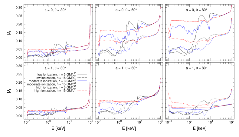
Figure 3.3: The reflected-only polarisation degree, $p_{\mathrm{r}}$, versus energy for the same parametric setup as in Figure 3.1, displayed in the same manner.

Figure 3.4: The total polarisation degree, $p$, versus energy for the same parametric setup as in Figure 3.1, displayed in the same manner.

The dependency of total polarisation degree on $h$ and $\theta$ is shown in more detail in Figures 3.5 and 3.6, integrated in various energy bins and for the neutral and ionized disc cases, respectively. Only if the lamp-post is located close to the event horizon, the relativistic effects depolarize significantly. Then the total polarisation departs from the otherwise monotonic dependency of $p(h)$, which is given by the reflection fraction and by the change of the dominant incident inclination angle for the local reflection tables. It was checked that the differences in these figures would be negligible, if the accretion disc was considered up to $r_{\mathrm{out}}=1000\,r_{\textrm{g}}$ (Podgorný et al., 2023a). The dependency of polarisation fraction on inclination is also nearly monotonic, apart from very high inclinations, where we obtained a drop in polarisation, thus a peak in polarisation is formed at $\theta\approx 65^{\circ}$. This is caused by the lower reflection fraction with respect to the primary at high heights and by the relativistic light-bending effects. Although the highly inclined views of the black hole’s vicinity would be observationally blocked by the dusty torus in AGNs, we keep the modeling discussion, because in Chapter 4 we will use KYNSTOKES for high $\theta$ as a spectropolarimetric model input of the equatorial illumination of such tori. At low $h$ and high $\theta$, the effects of different spin on the resulting polarisation are the clearest, due to the largest relativistic distortion in such scenarios. Comparing the two figures, which vary in disc ionization level, we can clearly see the energy independence of highly ionized reflection. The fast rotating black holes allow for higher reflection contribution (when the disc is considered down to ISCO, whose location changes with $a$) and increase of polarisation at low lamp-post heights and low or moderate inclinations. But at extreme inclinations, the black-hole spin rather acts as a depolarizer.

Figure 3.5: Top panel: the total average polarisation degree, $p$, versus height of the primary point-source above the disc for disc inclinations $\theta=30^{\circ}$ (left), $\theta=60^{\circ}$ (middle) and $\theta=80^{\circ}$ (right), $\Gamma=2$, unpolarized primary radiation, $M=1\times 10^{8}\,M_{\odot}$ and observed 2–10 keV flux $L_{\textrm{X}}/L_{\textrm{Edd}}=0.001$, i.e. neutral disc. We show cases of two black-hole spins $a=0$ (dashed) and $a=1$ (solid) and for energy bands $E\in[0.2,2]$ keV (black), $E\in[2,8]$ keV (blue), $E\in[8,12]$ keV (green), $E\in[12,20]$ keV (orange), and $E\in[20,50]$ keV (red). Bottom panel: the total average polarisation degree, $p$, versus disc inclination for heights of the primary point-source above the disc $h=3\textrm{ }r_{\textrm{g}}$ (left), $h=15\textrm{ }r_{\textrm{g}}$ (middle) and $h=100\textrm{ }r_{\textrm{g}}$ (right), for the same configuration as on the top panel.

Figure 3.6: The total average polarisation degree, $p$, versus energy for ionized disc ($M=1\times 10^{5}\,M_{\odot}$ and observed 2–10 keV flux $L_{\textrm{X}}/L_{\textrm{Edd}}=0.1$), otherwise for the same parametric setup as in Figure 3.5, displayed in the same manner.

Figure 3.7 shows the corresponding polarisation angle versus energy (the primary is considered unpolarized, so this quantity is identical for the reflected-only and total signal). For the lamp-post model, we obtain polarisation nearly parallel with the axis of symmetry of the system. Only small deviations occur in the continuum due to relativistic effects and in the spectral lines due to undefined local $\Psi$ for unpolarized fluorescent emission. The resulting polarisation angle orientation after the relativistic corrections is not obvious for high lamp-post heights, but we conclude that even in these cases the dominant single-scattering polarisation genesis occurs on the left and right sides of the equatorial disc from observer’s point of view, which symmetrically adds to net polarisation nearly parallel with the black-hole rotation axis. We note that in detailed relativistic studies of coronal Comptonization of disc seed photons (Ursini et al., 2022; Krawczynski and Beheshtipour, 2022), the resulting polarisation angle needs not to be either parallel or perpendicular to the axis of symmetry due to GR rotation effects. Figures A.4 and A.5 represent the same as in Figures 3.5 and 3.6, respectively, but for the net polarisation angle, where the subtle differences are clearer when plotted integrated in different energy bins.

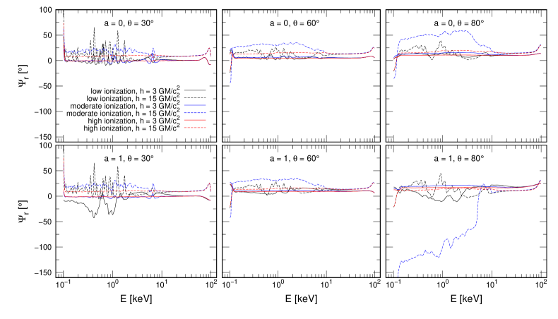
Figure 3.7: The reflected-only polarisation angle, $\Psi_{\mathrm{r}}$, versus energy for the same parametric setup as in Figure 3.1, displayed in the same manner.

We will now release the assumption of unpolarized primary, while keeping $\Gamma=2$, in order to discuss the effects of changing primary polarisation. The effect on the resulting spectra is negligible, hence we will only study the resulting polarisation state. We plot the cases of $p_{0}=0$ (purple lines in figures), $p_{0}=0.01$ and $\Psi_{0}=0^{\circ}$ (green lines in figures), $p_{0}=0.01$ and $\Psi_{0}=90^{\circ}$ (orange lines in figures), which are well within conservative estimates of coronal polarisation (Beheshtipour et al., 2017; Beheshtipour, 2018; Tamborra et al., 2018; Ursini et al., 2022; Krawczynski and Beheshtipour, 2022). We omit the results for highly ionized discs, because they show identical effects of changing incident polarisation, only with a generally higher contribution of reflected component with respect to the primary. Figure 3.8 shows for selected cases of $a$ and $\theta$ the reflected-only and total polarisation degree, and the reflected-only polarisation angle, for a neutral disc case and for two distinct lamp-post heights. The same simulations for different $a$ and $\theta$ are shown in Figures A.6–A.12, relatively to the case with unpolarized primary. We only provide here the usual six panels of different $a$ and $\theta$ in Figure 3.9 for the total value of polarisation angle for the neutral disc case, which is theoretically more interesting (see below).

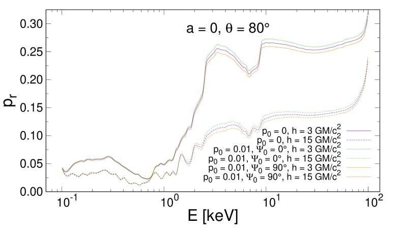
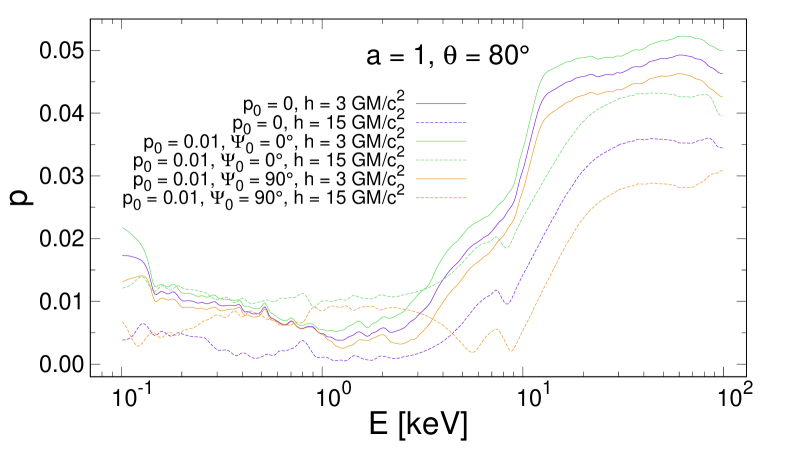
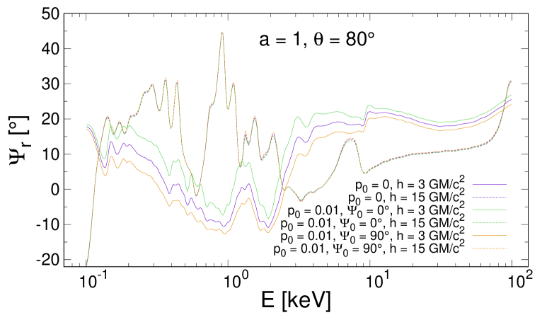
Figure 3.8: Top left: the reflected-only polarisation degree, $p_{\mathrm{r}}$, versus energy of the accretion disc for distant observer, obtained by KYNSTOKES for black-hole spin $a=0$, disc inclination $\theta=80^{\circ}$, $\Gamma=2$ and for the neutral disc ($M=1\times 10^{8}\,M_{\odot}$ and observed 2–10 keV flux $L_{\textrm{X}}/L_{\textrm{Edd}}=0.001$), using the STOKES local reflection model in the lamp-post scheme. We show cases of two different heights of the primary point-source above the disc $h=3\textrm{ }r_{\textrm{g}}$ (solid lines) and $h=15\textrm{ }r_{\textrm{g}}$ (dashed lines), and three different polarisation states of the primary source: $p_{0}=0$ (purple), $p_{0}=0.01$ and $\Psi_{0}=0^{\circ}$ (green), $p_{0}=0.01$ and $\Psi_{0}=90^{\circ}$ (orange). Top right: the total polarisation degree, $p$, versus energy for black-hole spin $a=1$, otherwise for the same parametric setup, displayed in the same manner. Bottom: the reflected-only polarisation angle, $\Psi_{\mathrm{r}}$, versus energy for black-hole spin $a=1$, otherwise for the same parametric setup, displayed in the same manner.

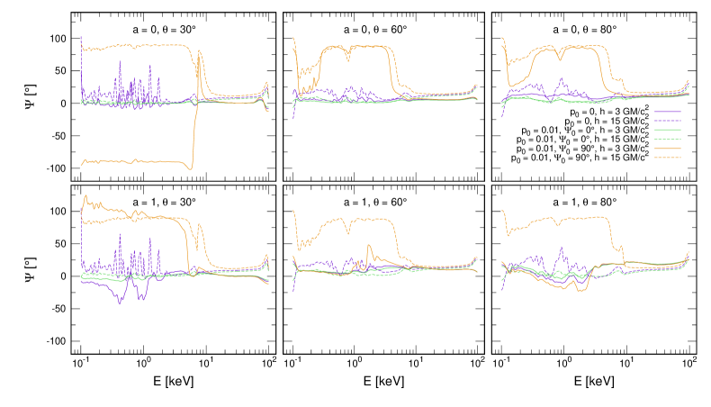
Figure 3.9: The total polarisation angle, $\Psi$, versus energy of the accretion disc for distant observer, obtained by KYNSTOKES for black-hole spins $a=0$ (top) and $a=1$ (bottom), disc inclinations $\theta=30^{\circ}$ (left), $\theta=60^{\circ}$ (middle) and $\theta=80^{\circ}$ (right), $\Gamma=2$ and neutral disc ($M=1\times 10^{8}\,M_{\odot}$ and observed 2–10 keV flux $L_{\textrm{X}}/L_{\textrm{Edd}}=0.001$), using the STOKES local reflection model in the lamp-post scheme. We show cases of two different heights of the primary point-source above the disc $h=3\textrm{ }r_{\textrm{g}}$ (solid lines) and $h=15\textrm{ }r_{\textrm{g}}$ (dashed lines), and three different polarisation states of the primary source: $p_{0}=0$ (purple), $p_{0}=0.01$ and $\Psi_{0}=0^{\circ}$ (green), $p_{0}=0.01$ and $\Psi_{0}=90^{\circ}$ (orange).

The resulting polarisation fraction (reflected-only or total) preserves qualitatively the same response at hard X-rays (where mostly Compton scattering is involved) to incident polarisation state for all studied cases. The values differ from the case with unpolarized primary by $\lessapprox 1\%$, with lower emergent polarisation for horizontally polarized incident photons (orange lines) and higher emergent polarisation for vertically polarized incident photons (green lines). If we test higher incident polarisation fraction, the resulting difference from the case with unpolarized primary (purple lines) scales linearly in the same qualitative direction. The differences are symmetric with respect to the unpolarized primary case, which has roots in the way that local reflection is constructed via (3.1). The emergent reflected-only polarisation angle is also symmetric with respect to the unpolarized case with differences $\lessapprox 1^{\circ}$. The symmetry is broken when the primary radiation is added to the total polarisation angle and degree, especially at soft X-rays. This is seen in Figure 3.9, where the orange lines drawn for horizontal incident polarisation, deviate significantly at soft X-rays from the parallel polarisation inherent to the reflected emission. At soft X-rays for a neutral disc, the reflected flux contribution is not significant with respect to the primary flux and the polarisation degree also tends to unite at $1\%$, if prescripted for the primary. Figure A.13 shows that the polarisation angle transition for $p_{0}=0.01$ and $\Psi_{0}=90^{\circ}$ needs not to always occur in the 2–8 keV important for IXPE or eXTP. It depends on the chosen $h$ and $\theta$.

Let us briefly examine the role of $\Gamma$. Apart from the slope of primary radiation, which weights differently polarized photons at different energies, the disc ionization is affected. The local ionization parameter given by (1.18) is still changing with $\Gamma$ for a fixed normalization given by $L_{\textrm{X}}/L_{\textrm{Edd}}$ and $M$ and fixed $n_{\textrm{H}}$. Higher photon index makes the spectral lines and absorption in the reprocessed emission more pronounced (depending on the energy band), since less energetic photons ionize the disc. This imprints to the energy dependence of polarisation degree at infinity. For higher $\Gamma$, we see a slight depolarisation in between $0.8$–$3$ keV where the polarisation degree with energy had a nearly constant curve for $\Gamma=2$ for highly ionized (red curves) cases in Figures 3.3 and 3.4. The effect is, however, lower with the new code than reported in Podgorný et al. (2023a) due to higher interpolation precision, using the newer version of the TITAN and STOKES tables. We notice an overall increase of polarisation for $a=0$ and decrease for $a=1$ between $\Gamma=2$ and $\Gamma=3$, as relativistic effects play a role. We provide the same total polarisation degree versus inclination and lamp-post height as in Figure 3.6 (showing the results for $\Gamma=2$) but for $\Gamma=3$ in Figure 3.10. The $y$-axis is extended with respect to the previously shown case with $\Gamma=2$.

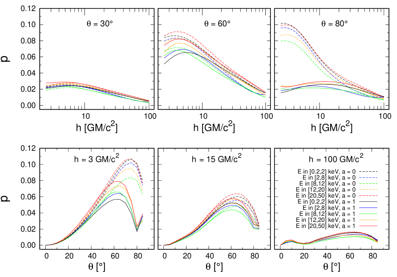
Figure 3.10: The total average polarisation degree, $p$, versus energy for $\Gamma=3.0$, otherwise for the same parametric setup as in Figure 3.6, displayed in the same manner.

Finally, we will investigate the role of disc truncation for polarisation gain by reflection, which especially in the pure lamp-post model should introduce effectively a new geometry of emission. As described in Chapter 1, determination of the inner disc radius can be of vital importance for our understanding of the accretion mechanisms. This holds not only for the hard spectral state of XRBs, where the disc is believed to be significantly truncated. The effects of reducing spatial symmetry for reflection inside the system in this way are similar in polarisation induction across all X-ray energies, so we will only provide the integrated result in 2–8 keV band, important for the IXPE and eXTP missions. For three different inclinations and various cases of incident polarisation, we will plot the reflected-only and total polarisation degree and angle versus $r_{\textrm{in}}$, in between ISCO and $100\,r_{\textrm{g}}$. Since wide range of disc truncations is studied, we extend the outer disc radius to $r_{\mathrm{out}}=1000\,r_{\textrm{g}}$ specifically for these calculations. We also add the corresponding reflection fraction $R_{\textrm{f}}$, i.e. the observed energy-integrated reflected-only flux divided by the observed energy-integrated total flux in 2–8 keV. The dependencies are similar for different $a$, so we show only the results for $a=1$, which is more interesting than a Schwarzschild black hole, because it allows to examine spatial regions closer to the event horizon, assuming a standard accretion disc with sharp truncation on the inner side.

Figures 3.11 and A.15 show the results for $h=3\,r_{\textrm{g}}$ and $h=15\,r_{\textrm{g}}$, respectively, for highly ionized disc. The same for nearly neutral disc is shown in Figures A.16 and A.17. The more we truncate the disc, the more we limit the allowed scattering space and the higher polarisation we obtain. The trade-off for more detectable higher polarisation fraction is, however, the reflection fraction, which obviously decreases with truncation for lamp-post coronae. For highly ionized discs, the increase of reflected-only polarisation degree with $r_{\textrm{in}}$ saturates and at low lamp-post heights, we observe again a decrease of polarisation degree for $r_{\textrm{in}}\gtrapprox 30\,r_{\textrm{g}}$. The lower the $R_{\textrm{f}}$ is, the more the total polarisation result for a distant observer reaches the polarisation prescription at the lamp-post. The polarisation change between the lamp-post and the observer is not significant (see Appendix C). All of the disc truncation effects are inclination dependent.

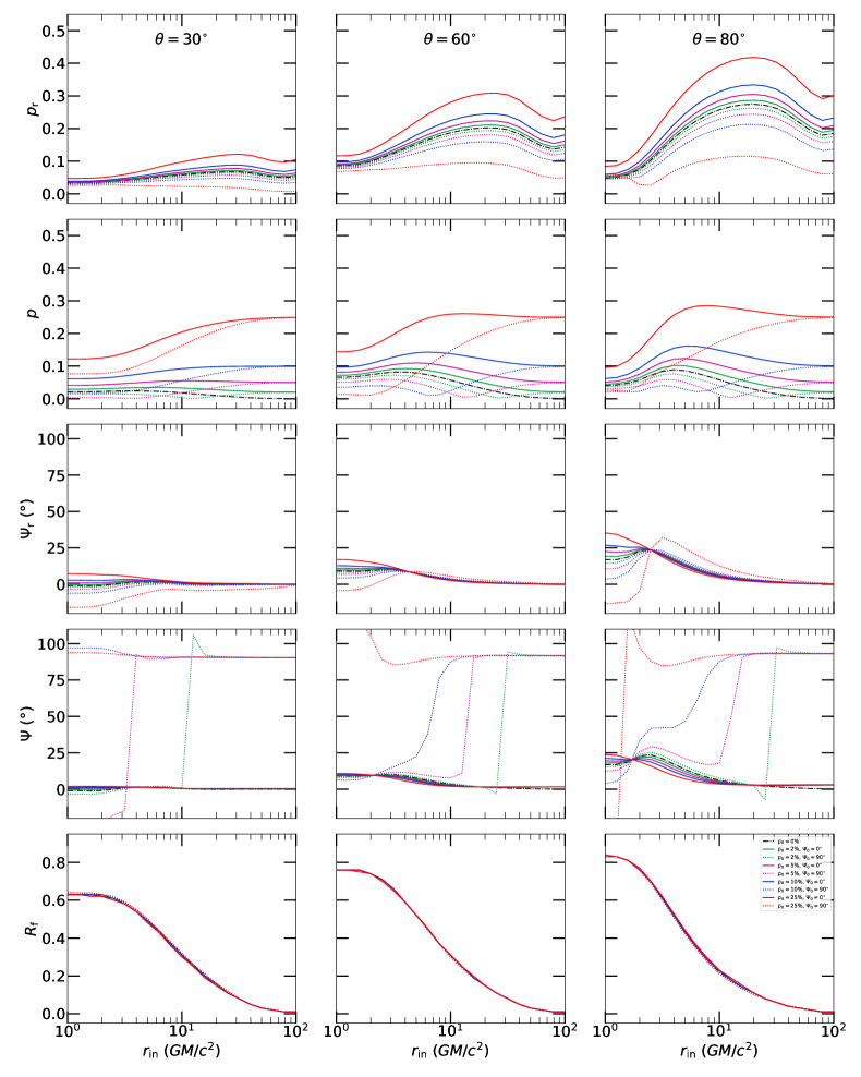
Figure 3.11: The spectropolarimetric output of KYNSTOKES in the lamp-post regime with respect to disc truncation, integrated in 2–8 keV band. From top to bottom we show the reflected-only polarisation degree, $p_{\textrm{r}}$, the total polarisation degree, $p$, the reflected-only polarisation angle $\Psi_{\textrm{r}}$, the total polarisation angle, $\Psi$, and the reflection fraction, $R_{\textrm{f}}$, all as a function of the inner disc radius $r_{\textrm{in}}$. Various cases of the primary polarisation state are shown in the color code and line style. We show the results for $\Gamma=2$, $a=1$ and $\theta=30^{\circ}$ (left column), $\theta=60^{\circ}$ (middle column) and $\theta=80^{\circ}$ (right column).

3.1.2 Comparison to other models

Let us compare the lamp-post results within the same KY relativistic integration, but using different local reflection computations. We will now assume again the full disc without any truncation. For this we will use the KYNLPCR routine (courtesy of Michal Dovčiak) that assumes reflection for a purely neutral disc, computed with NOAR (Różańska et al., 2002), and the KYNXILLVER routine (courtesy of Michal Dovčiak) that assumes the XILLVER spectral reflection tables (García et al., 2013), which we juxtaposed locally to the TITAN and STOKES tables in Section 2.1.2. Figure A.14 shows the relativistically integrated spectra from KYNSTOKES, KYNLPCR and KYNXILLVER routines for unpolarized primary with $\Gamma=2$, $h=3\textrm{ }r_{\textrm{g}}$, two cases of disc ionization, two black-hole spins and three inclinations. The largest differences occur, as anticipated from the local reflection tables, in the soft X-rays. KYNLPCR underpredicts flux contribution for the more realistic nearly neutral disc below 1 keV for $a=0$ and below 10 keV for $a=1$. The KYNSTOKES spectral results are systematically higher normalized than the KYNXILLVER results for the low ionization cases, and lower normalized than the KYNXILLVER results for the high ionization cases. The difference may be also due to angular treatment of the local reflections. Three angles are considered in the TITAN and STOKES tables, compared to the isotropically irradiated and azimuthally averaged reflection in XILLVER.

The KYNLPCR routine, with which the results in Dovčiak et al. (2011) were computed, contains also local reflection polarisation calculations through the single-scattering Chandrasekhar’s formulae 1.39. Figures 3.12 and 3.13 provide comparisons with KYNSTOKES of the reflected-only and total polarisation degree versus energy, respectively, for changing incident polarisation, two black-hole spins, three inclinations, neutral accretion disc ($M=1\times 10^{8}\,M_{\odot}$ and observed 2–10 keV flux $L_{\textrm{X}}/L_{\textrm{Edd}}=0.001$ for KYNSTOKES), unpolarized primary with $\Gamma=2$ and $h=3\textrm{ }r_{\textrm{g}}$. The same for reflected-only and total polarisation angle is shown in Figures 3.14 and 3.15, respectively. The relativistic effects are the same for both codes. But as shown in Figure 2.4, at X-ray energies $\gtrapprox 10$ keV the locally induced polarisation by single-scattering significantly overpredicts the resulting polarisation. We now see the full energy dependence, including relativistic effects. The small differences in local reflection polarisation angle result in nearly identical polarisation orientation predictions for the distant observer. The only exception being the initially horizontally polarized primary radiation, which in the case of KYNLPCR is always dominating over the reflection in soft X-rays, as there the reflection component is practically absent.

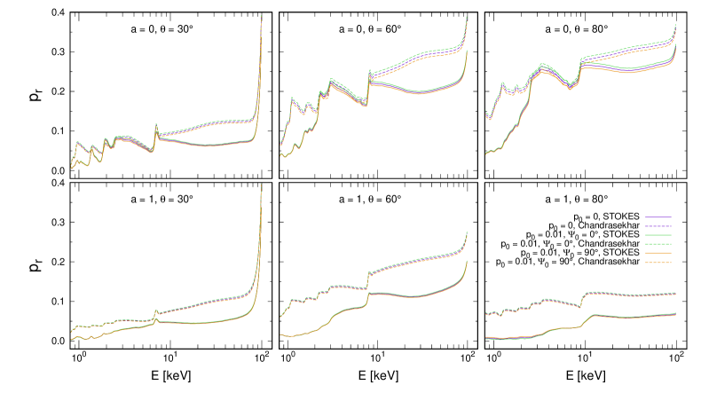
Figure 3.12: The reflected-only polarisation degree versus energy, $p_{\mathrm{r}}$, of the accretion disc for distant observer in the lamp-post scheme for black-hole spins $a=0$ (top) and $a=1$ (bottom), disc inclinations $\theta=30^{\circ}$ (left), $\theta=60^{\circ}$ (middle) and $\theta=80^{\circ}$ (right), $\Gamma=2$, height of the primary point-source above the disc $h=3\textrm{ }r_{\textrm{g}}$ and neutral disc (for $M=1\times 10^{8}\,M_{\odot}$ and observed 2–10 keV flux $L_{\textrm{X}}/L_{\textrm{Edd}}=0.001$). We compare cases of KY disc integration with the STOKES local reflection tables (solid lines) and NOAR local reflection tables with Chandrasekhar’s analytical approximation for polarisation (dashed lines), and three different polarisation states of the primary source: $p_{0}=0$ (purple), $p_{0}=0.01$ and $\Psi_{0}=0^{\circ}$ (green), $p_{0}=0.01$ and $\Psi_{0}=90^{\circ}$ (orange).

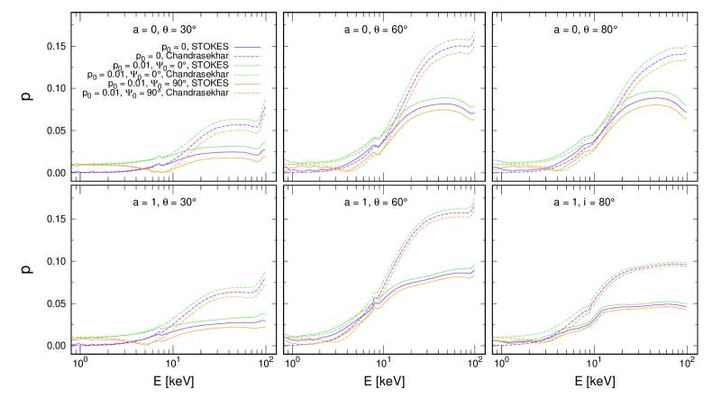
Figure 3.13: The total polarisation degree, $p$, versus energy for distant observer for the same parametric setup as in Figure 3.12, displayed in the same manner.

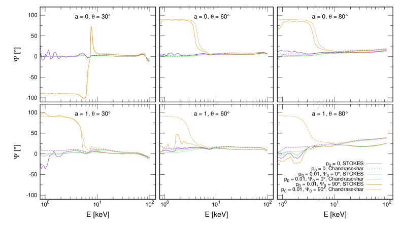
Figure 3.14: The reflected-only polarisation angle, $\Psi_{\mathrm{r}}$, versus energy for distant observer for the same parametric setup as in Figure 3.12, displayed in the same manner.

Figure 3.15: The total polarisation angle, $\Psi$, versus energy for distant observer for the same parametric setup as in Figure 3.12, displayed in the same manner.

Direct comparisons with the RELXILL relativistic lamp-post implementation of XILLVER tables would require a detailed analysis of normalization in the first place. It would, however, be a valuable next step, because the original RELXILL codes (García et al., 2014; Dauser et al., 2014) now include returning radiation (Dauser et al., 2022). Apart from the critical assumption of lamp-post isotropic emission and apart from many improvements already suggested for the local reflection tables in Section 2.1.2, it is also highly desirable to implement higher-order reflections in KYNSTOKES and cross-validate the pioneering study of Dauser et al. (2022) from the spectroscopic point of view. The effects of returning radiation on the resulting polarisation can be at least qualitatively predicted, based on the works of Schnittman and Krolik (2009, 2010); Taverna et al. (2020), which were carried for returning radiation effects on polarisation of thermal radiation of accretion discs in XRBs, assuming the diffuse Chandrasekhar’s formulae for reflection.

It is argued in Dauser et al. (2022) that the returning radiation provides the largest difference for high black-hole spins ($a\gtrapprox 0.9$) and low lamp-post heights ($h\lessapprox 5\,r_{\textrm{g}}$), due to contributions from the inner-most parts of the disc ($r\lessapprox 10\,r_{\textrm{g}}$). Although azimuthally dependent, the net polarisation fraction given by the self-irradiation in Schnittman and Krolik (2009, 2010) (without and with an extended corona considered) was $\approx 10\%$ with polarisation angle parallel to the axis of symmetry. Both were constant in energy. In KYNSTOKES, the resulting polarisation tends to be aligned with the principal axis and of the order of a few %. Despite the different source of irradiation in Schnittman and Krolik (2009, 2010) than we would have for once reprocessed radiation returning to the disc, we could thus expect in our cases an additional polarisation effect, rather than depolarisation. Nonetheless, a detailed calculation would have to prove such predictions, because the local flux angular distribution could play a role, as well as the relative flux contributions onto and from different disc regions, as well as the spectral shape of a reprocessed power-law, compared to the thermally radiating discs. Moreover, in Section 3.1.1 we proved the non-negligible impact of incident polarisation on the integrated reprocessed result.

3.2 The sandwich coronal model

Here we consider the extended corona with negligible height, sitting on top of the reflecting accretion disc, as described in Section 1.5.2. As there is no photon travelling considered between the source of X-rays and the disc, the total emission is given by the same geodesics from the equatorial plane, either from the primary source, or from the reprocessed radiation given by the TITAN and STOKES local reflection tables, described in Section 2.1 and considered in the model at the same equatorial location, corotating with the source of emission in the equatorial plane. Locally, we uniformly integrate the reflection tables in the incident angles $\mu_{\textrm{i}}$ and azimuthal emission angles $\Phi_{\textrm{e}}$, to account for the diffuse character of the source. The disc is also here assumed to have a constant radial density profile with $n_{\textrm{H}}=10^{15}\ \textrm{cm}^{-3}$, according to the local reflection tables again. Equivalently to the previous section, the disc inner radius $r_{\mathrm{in}}$ is fixed at the ISCO and $r_{\mathrm{out}}=400\,r_{\textrm{g}}$, if not stated otherwise. We will again study the case of reflected-only radiation with $N_{\textrm{p}}/N_{\textrm{r}}=0$ and the case of added primary source with $N_{\textrm{p}}/N_{\textrm{r}}=1$, normalized according to the local reflection tables and the radial emissivity profile. We stress that the model in this setup is not realistic mainly because the coronal photons re-processed inside the disc would inevitably be re-processed again in the corona before reaching the observer. Hence, the results of this model should be viewed as an extreme case of an extended corona, to which a moderately extended lamp-post model would be converging for ever larger (and already unrealistic) sizes. In other words, as a direction of results (assuming some monotony) discussed in Section 3.1, if we increased the size of the lamp-post corona, which is in practice difficult, as our computational approach relies on symmetry simplifications. We refer to the X-ray polarisation studies of Poutanen and Svensson (1996); Schnittman and Krolik (2010); Krawczynski and Beheshtipour (2022) that deal with the subsequent re-processing in the corona in sandwich geometries.

The radial emissivity profile of the primary source is given by the power-law index $q$. In order to not further complicate the discussion with changing the physical scale units with $M$, we fix the black-hole mass at $M=2\times 10^{6}M_{\odot}$. The user-defined observed 2–10 keV flux $L_{\textrm{X}}/L_{\textrm{Edd}}$ in KYNSTOKES is considered as global, meaning this value irradiates each ring surface area of $2\pi r\textrm{d}r$ given by the chosen binning, multiplied by $r^{-q}$. The local reflection ionization parameter is scaled accordingly from $\xi_{0}$ defined at $r=6\,r_{\textrm{g}}$, which is available above ISCO for any black-hole spin. In order to reasonably compare our results to the lamp-post scenario where the radial irradiation profile is given, we chose the $q=3$, $a=0$ and $\theta=30^{\circ}$ values as default and searched for such values of $L_{\textrm{X}}/L_{\textrm{Edd}}$ that produce similar levels of low, moderate and high disc ionizations, as obtained in Section 3.1.1 for the KYNSTOKES lamp-post variant. This turns out to be $L_{\textrm{X}}/L_{\textrm{Edd}}|_{q=3,\theta=30^{\circ}}=10^{-5}$, $L_{\textrm{X}}/L_{\textrm{Edd}}|_{q=3,\theta=30^{\circ}}=10^{-2}$ and $L_{\textrm{X}}/L_{\textrm{Edd}}|_{q=3,\theta=30^{\circ}}=10^{2}$ for the low, moderate and high ionization cases, respectively. Due to the chosen fixation of $\xi_{0}$ at $r=6\,r_{\textrm{g}}$ we then used $L_{\textrm{X}}/L_{\textrm{Edd}}$ for different $q$ and $\theta$ renormalized according to

$$\left.L_{\textrm{X}}/L_{\textrm{Edd}}\right|_{q,\theta}=\frac{\left.L_{\textrm{X}}/L_{\textrm{Edd}}\right|_{q^{\prime},\theta^{\prime}}r^{q-q^{\prime}}(2-q^{\prime})\cos{(\theta)}(r_{\textrm{out}}^{2-q}-r_{\textrm{in}}^{2-q})}{(2-q)\cos{(\theta^{\prime})}(r_{\textrm{out}}^{2-q^{\prime}}-r_{\textrm{in}}^{2-q^{\prime}})}\textrm{ ,}$$ (3.3)

where $r=6\,r_{\textrm{g}}$, $r_{\textrm{in}}=1\,r_{\textrm{g}}$, $r_{\textrm{out}}=400\,r_{\textrm{g}}$, $q^{\prime}=3$ and $\theta^{\prime}=30^{\circ}$. It accounts for the difference in radial emissivity, hence similar ionization features are produced.

Figures 3.16 and 3.17 show the reflected-only and total spectra, respectively, for the three cases of disc ionization, two values of $q$, two spins and three inclinations, all for unpolarized primary with $\Gamma=2$. We again compensate for the primary power-law slope and renormalize to the value at 50 keV to see the spectral features clearly. Comparing to Figures 3.1 and 3.2 for the lamp-post model, we see similar effects of relativistic integration across the disc. The radial emissivity index $q$ plays similar role for the sandwich corona as the height $h$ for lamp-post. The lower the height, the steeper irradiation profile we obtain for the lamp-post. At $r\gtrapprox 50\,r_{\textrm{g}}$, the irradiation profile for lamp-post models approaches $q=3$ for any $h$ (Dovčiak et al., 2014). Only for high black-hole spin and high inclinations the relativistic effects on the primary radiation are significant enough that the two geometries produce qualitatively different spectral profiles in our model.

Figure 3.16: The reflected-only spectra of the accretion disc for distant observer, $EF_{\textrm{E,r}}$, normalized to value at 50 keV, obtained by KYNSTOKES for black-hole spins $a=0$ (top) and $a=1$ (bottom), disc inclinations $\theta=30^{\circ}$ (left), $\theta=60^{\circ}$ (midlle) and $\theta=80^{\circ}$ (right), $\Gamma=2$, $M=2\times 10^{6}\,M_{\odot}$, and unpolarized primary radiation, using the STOKES local reflection model in the extended coronal scheme. We show cases of two different radial illumination power-law indices $q=1.5$ (dotted lines) and $q=3.0$ (solid lines), and neutral disc (observed 2–10 flux $L_{\textrm{X}}/L_{\textrm{Edd}}\approx 10^{-5}$, see text for details, black lines), moderately ionized disc (observed 2–10 flux $L_{\textrm{X}}/L_{\textrm{Edd}}\approx 10^{-2}$, see text for details, blue lines) and highly ionized disc (observed 2–10 flux $L_{\textrm{X}}/L_{\textrm{Edd}}\approx 10^{2}$, see text for details, red lines).

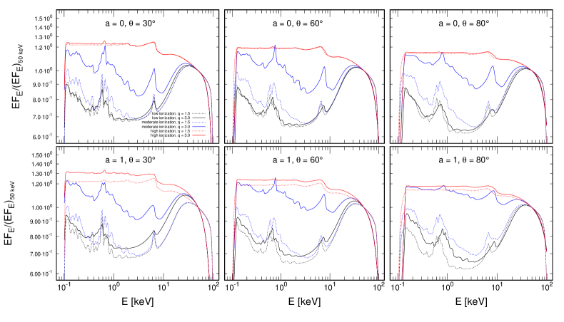
Figure 3.17: The total spectra of the accretion disc for distant observer, $EF_{\textrm{E}}$, normalized to value at 50 keV, for the same parametric setup as in Figure 3.16, displayed in the same manner.

Polarisation signatures, on the contrary, vary significantly. Figures 3.18 and 3.19 provide the corresponding reflected-only and total polarisation profile with energy, respectively. We obtain almost full depolarisation in the soft X-rays. In the 1–100 keV range, the reflected-only results follow the dependency of poalrization with energy of the local reflection tables (cf. Figure 2.1), preserving the dip of reduced polarisation in the iron line complex at 6–7 keV. The absorption-induced peak in reflection that forms in 1–20 keV range is skewed towards higher energies when the primary radiation is added, because this coronal emission is unpolarized and with decreasing flux contribution with energy dilutes polarisation more at lower energies. If different $\Gamma$ is assumed, the reflected polarisation degree is diluted by the energy dependence of the unpolarized primary accordingly.

Figure 3.18: The reflected-only polarisation degree, $p_{\mathrm{r}}$, versus energy for the same parametric setup as in Figure 3.16, displayed in the same manner.

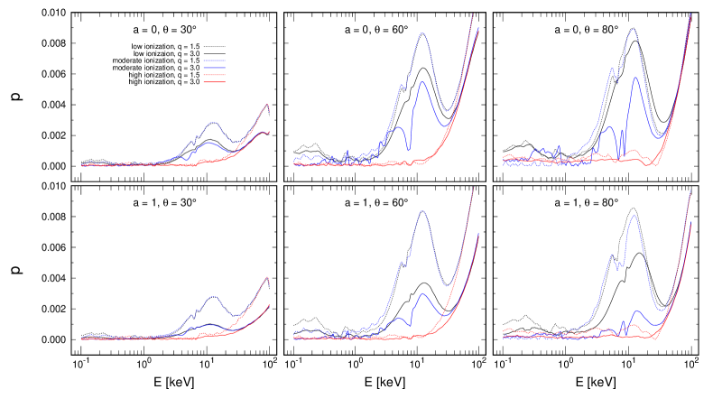
Figure 3.19: The total polarisation degree, $p$, versus energy for the same parametric setup as in Figure 3.16, displayed in the same manner.

The maximum amplitude of reflected-only polarisation in the X-rays is only $\approx 8\%$ in the most favorable configurations, while the majority of the parameter space ends up below $\approx 2\%$. We note that the studied sandwich model is extremely simplistic and we would expect yet another reflected-only and total polarisation result, if a different coronal model was assumed. More sophisticated coronal studies (Ursini et al., 2022; Krawczynski and Beheshtipour, 2022; Krawczynski et al., 2022; Gianolli et al., 2023; Tagliacozzo et al., 2023) typically result in higher polarisation of direct coronal emission in the slab models compared to lamp-posts of non-negligible size, because with respect to the disc seed photons and the observer, the slab model represents the more asymmetric situation. For reflection of coronal radiation off the disc to the observer, the lamp-post scenario is in turn the more asymmetric variant for a distant observer.

Figure 3.20 shows the corresponding polarisation angle with energy. Since we study the unpolarized primary case, the plot is the same with the primary radiation or without. For the sandwich model, we observe typically a dominant polarisation perpendicular to the axis of symmetry in reflection. The reason for this is the isotropic illumination of the disc, which locally produces polarisation rather parallel with the disc (see Sections 1.5.1 and 2.1). Only for the highest inclinations the prevailing polarisation position angle for an observer at spatial infinity is rather parallel with the axis of symmetry for soft and mid X-rays and for moderate or highly ionized cases. The value where the switch in resulting polarisation occurs is generally also dependent on $\Gamma$. For the direct coronal emission, we expect, however, quite the opposite than from reflection off the disc: the lamp-post coronae typically produce polarisation perpendicular to the rotation axis, while the sandwich models typically produce polarisation parallel to the principal axis (Ursini et al., 2022; Krawczynski and Beheshtipour, 2022; Krawczynski et al., 2022; Gianolli et al., 2023; Tagliacozzo et al., 2023).

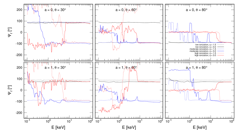
Figure 3.20: The reflected-only polarisation angle, $\Psi_{\mathrm{r}}$, versus energy for the same parametric setup as in Figure 3.16, displayed in the same manner.

We studied the dependency on changing primary polarisation again for the cases of $1\%$ polarized primary with either parallel or perpendicular polarisation, juxtaposed to the unpolarized primary case. This is shown in Figures A.18–A.25, for the reflected-only and total polarisation degree and angle and for the neutral and ionized disc. The effects of changing primary polarisation on spectra are again negligible. In most cases, we obtain the highest reflection-induced polarisation for the originally horizontally polarized primary. However, the role of the three cases in the net amplitude of reflected polarisation changes with energy. The added primary radiation does not always polarize or depolarize in the prescribed way at the equatorial plane, because each emission region is (i) weighted differently due to radial emissivity profile, (ii) weighted differently due to the relativistic transfer function, (iii) obtaining a different poalrization angle change from the original value in the equatorial plane due to GR effects between the disc and the observer, which results in net depolarisation for a distant observer.

We briefly examined also the dependency on disc truncation by extending the outer disc radius to $r_{\mathrm{out}}=1000\,r_{\textrm{g}}$ and plotting the polarisation quantities and $R_{\textrm{f}}$ with respect to $r_{\textrm{in}}$ similarly to the lamp-post results in Section 3.1.1. Figure A.26 shows a representative case of $a=1$, $q=3$ and highly ionized disc reflection for three different inclinations. For the extended corona, the results depend strongly on the chosen primary emission model. For our choice, we do not obtain almost any change of $R_{\textrm{f}}$ with $r_{\textrm{in}}$. The polarisation fraction only slightly increases with $r_{\textrm{in}}$. The resulting polarisation angle is slightly rotated, depending on the inner disc extension below $10\,r_{\textrm{g}}$ due to the impact of gravity on the polarisation angle along the photon’s trajectory.

Chapter 4 Contribution of distant components of accreting systems

In this chapter, we continue the trend of zooming out in physical size and we model the X-ray polarisation properties of distant circumnuclear components of accreting compact objects. Wedge-like and toroidal shapes will be assumed for studies of equatorial reprocessing first, which are parametrized in Figure 4.2. Wedge-like equatorial scatterers combined with conical polar outflows will also be studied at the end of this chapter, as in Figure 4.2. The details of the modeling will be given as part of the results below.

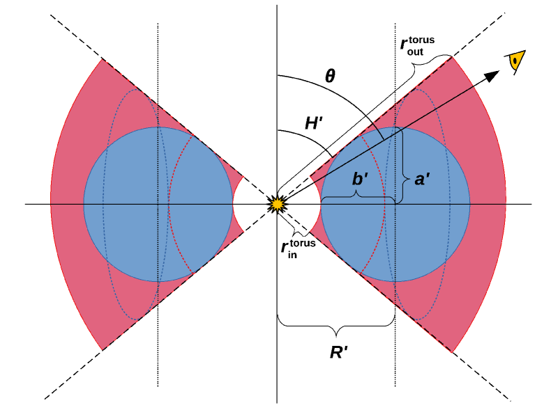
Figure 4.1: Wedge-shaped, circular and elliptical toroidal structures, equatorially covering the central source of isotropic power-law emission. These homogeneous and static distant cold media are rotationally symmetric around the principal axis and mirror symmetric with respect to the equatorial plane. Image adapted from Podgorný et al. (2023c).

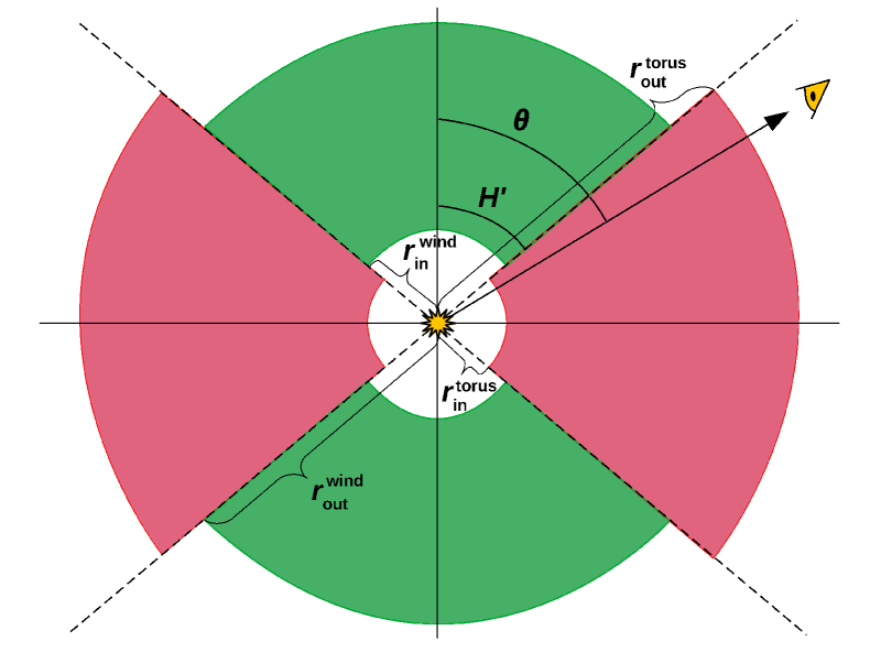
Figure 4.2: The complete AGN model assuming polar winds in rotationally symmetric wedge-like cones around the principal axis. Wedge-like equatorial tori are kept glued to the polar scatterers. We assume a disc-corona source of emission in the lamp-post geometry located in the center. Image adapted from Podgorný et al. (2024).

4.1 Reprocessing in equatorial obscurers
with Monte Carlo simulations

We begin with studying reprocessing in regions residing symmetrically around and near the equatorial plane. As suggested in Chapter 1, these can be either the parsec-scale dusty tori of AGN, or more ionized outflows in funnel-like structures, originating from the outer accretion discs of stellar-mass compact objects. The results presented in this section were produced with STOKES (v2.07, identical with the version used for production of results in Marin et al., 2018a, b) and published in Podgorný et al. (2023c), only with a different notation. The simplification with respect to the STOKES results presented in Chapter 2 is that partial ionization is treated only by means of uniform free-electron density. The free electrons are added on top of uniformly distributed atomic species with $A_{\textrm{Fe}}=1$ and solar abundances from Asplund et al. (2005). No clumpiness or ionization fronts are taken into account and no radiative transfer code is linked to the MC simulation to solve for true ionization structure. Hence the reflected continuum spectra show a typical $\sim-E^{-3}$ decay towards the soft X-rays, owing to photoelectric absorption in cold media mixed with electrons of diverse origin (owing to e.g. streams following magnetic fields). With respect to a proper treatment of ionization we preserve in reflection the total flux amplification by means of scattering on free and bound electrons, but regarding energy dependence of the reflected spectra, we introduce artificially more absorption at soft X-rays. The same holds for transmission through a patch of matter: scattering effects follow the density of free electrons, but the energy dependence of absorption is biased towards the soft X-rays. In any case, this leads to artificially enhanced polarisation towards the soft X-rays. Comptonization, synchrotron and thermal radiation effects are neglected too, which is more justifiable for the distant regions than for the studies of the inner disc-corona system. We show MC results obtained only with STOKES and no other code is used, in order to discuss the main principles and diversity of possible results.

We assume a simple isotropic static source of arbitrarily polarized power-law radiation in the center of coordinates, representing the disc-corona region shrunk to negligible size. In order to examine the effects of changing primary irradiation, we simulated unpolarized and $2\%$ polarized primary parallelly or perpendicularly to the axis of symmetry for a range of photon indices: $1.2\leq\Gamma\leq 2.8$. We preserve axial symmetry, mirror symmetry with respect to the equatorial plane, and homogeneous density along the scattering region, as it is already nearly impossible to cover such reduced parameter space in full scope within one discussion section. The scattering regions neither possess any bulk motion with respect to the source of radiation. No polar scattering regions are included for results presented in this section. The photons can change direction, or be truly absorbed anywhere in the equatorial scattering region. They can also escape the reprocessing material and encounter it again at a different surface location. Thus, the model takes into account the effects of self-irradiation.

At first, we plan to examine the interaction of light and matter in the circumnuclear components theoretically. Thus, we forbid the registration of direct radiation for the following plots, in order to understand the main driving mechanisms inside the system for reflection-induced polarisation. This is important to mention especially with respect to the type-1 viewing angles, where we aim to examine the effects of only the reprocessed light. We will add direct radiation to these simulations in Chapter 5 where we will apply the equatorial reprocessing MC model to the interpretation of IXPE observations of Cygnus X-3, an XRB caught in hard and intermediate spectral states. This will allow us to evaluate the impact of direct radiation more clearly with respect to this section. It will also allow us to discuss the results from a different perspective and to assess the model sensitivity to a few other assumptions.

Distinct geometrical variants of the equatorial scattering region are considered, as is shown in Figure 4.2. We study

• Case A: a wedge-shaped torus defined by $r_{\textrm{in}}^{\textrm{torus}}$, $r_{\textrm{out}}^{\textrm{torus}}$ and its half-opening angle $H^{\prime}$;

• Case B: a true geometrical torus with an elliptical profile given by the parameters $R^{\prime}$, $a^{\prime}$ and $b^{\prime}$;

• Case C: a subcase of Case B representing a torus with circular profile, i.e. when $a^{\prime}=b^{\prime}$.

When there is a comparison between the wedge-shaped and circular or elliptical tori, we link $r_{\textrm{in}}^{\textrm{torus}}$ of the wedge to the $r_{\textrm{in}}^{\textrm{torus}}=R^{\prime}-b^{\prime}$ inner-most equatorial circle of the circular or elliptical tori, to examine the changing convexity or concavity effects of the inner toroidal wall located in the same place in equatorial plane. For Case B, we set $b^{\prime}$ relative to $R^{\prime}$ and study various eccentricities from prolate to oblate tori: $b^{\prime}=R^{\prime}/8$, $b^{\prime}=R^{\prime}/4$, $b^{\prime}=R^{\prime}/2$, $b^{\prime}=3R^{\prime}/4$, where $R^{\prime}=b^{\prime}+r_{\textrm{in}}^{\textrm{torus}}$ for a fixed $r_{\textrm{in}}^{\textrm{torus}}$. Therefore, by changing the eccentricity, we also trace the effects of changing curvature of the inner reflecting surface. For a given $H^{\prime}$ measured from the pole, we then define for Case B the parameter $a^{\prime}$ self-consistently via

$$a^{\prime}=\tan\left(\frac{\pi}{2}-H^{\prime}\right)\sqrt{R^{\prime 2}-b^{\prime 2}}\textrm{ .}$$ (4.1)

Case C is denoted as a special case of the elliptical torus, because it will be used frequently in the follow-up section as a referential MC case study for comparisons with a different model. In addition, for Case C we also compute $a^{\prime}=b^{\prime}$ in a different way than for the Case B. For Case C

$$a^{\prime}=b^{\prime}=r_{\textrm{in}}^{\textrm{torus}}\frac{\cos{H^{\prime}}}{1-\cos{H^{\prime}}}\textrm{ ,}$$ (4.2)

where again $r_{\textrm{in}}^{\textrm{torus}}$ is given. In this way, for a fixed $H^{\prime}$, when comparing Case C to Cases B with any $b^{\prime}/R^{\prime}$ ratio, the torus radii $R^{\prime}$ are different, but the inner boundary remains the same between the two cases. Case B would equal Case C, if $b^{\prime}/R^{\prime}=\cos{H^{\prime}}$. We always directly compare the geometrical shapes with the same half-opening angle $H^{\prime}$ and observer’s inclination $\theta$.

The default parameter values are physically and observationally motivated (see Goosmann and Gaskell, 2007; Marin et al., 2018a, b, and references therein). We choose $r_{\textrm{in}}^{\textrm{torus}}=0.05$ in this section, representing a fraction of a parsec for an AGN torus inner boundary, or an outer edge of an accretion disc around supermassive black hole. Nevertheless, the units are arbitrary and the results can be used for orders-of-magnitude lighter objects, as for polarisation genesis in this approach only the relative sizes inside the system matter. For Case A we set $r_{\textrm{out}}^{\textrm{torus}}=10$, representing the outermost AGN torus boundary in parsecs. The relative distance of the outer edge of the reprocessing region to the center with respect to characteristic sizes plays, however, little role compared to the inner-boundary location and shape, where the photons exhibit their first scatterings, which are determinative for the total geometry. This holds as long as the column densities of the entire scattering and absorption region are kept constant and high enough.

We refer to a “type-1” observer when $\theta<H^{\prime}$. We refer to a “type-2” observer when $\theta>H^{\prime}$. We will examine the output in 20 emission inclination bins linearly spaced in $0\leq\cos{\theta}\leq 1$ and one averaged azimuthal bin. Due to high expected absorption at soft X-rays, we consider only 200 logarithmically spaced energy bins between 1 and 100 keV. We do not consider any relativistic effects, so the result is either parallelly or perpendicularly polarized with respect to the principal axis due to meridional mirror symmetry from the observer’s point of view. Hence, we will adopt the notation of positive or negative polarisation degree, if the polarisation angle is parallel or perpendicular to the central axis of symmetry, respectively.

We display the results with respect to equatorial column density of neutral hydrogen $N_{\textrm{H}}^{\textrm{eq}}=n_{\textrm{H}}L$, which is given by the uniform neutral hydrogen density $n_{\textrm{H}}$ and $L=r_{\textrm{out}}^{\textrm{torus}}-r_{\textrm{in}}^{\textrm{torus}}$ for Case A and $L=2b^{\prime}$ for Cases B and C. We also define the equatorial Thomson optical depth $\tau_{\textrm{e}}^{\textrm{eq}}=\sigma_{\textrm{T}}n_{\textrm{e}}L$, where $n_{\textrm{e}}$ is the uniform density of free electrons in the scattering region. We work with three cases of partial ionization, referring to them as “low”, “moderate” and “high” ionization level ($\tau_{\textrm{e}}^{\textrm{eq}}=0.07,0.7,7$, respectively, for $N_{\textrm{H}}^{\textrm{eq}}=10^{25}\textrm{ cm}^{-2}$ and $\tau_{\textrm{e}}^{\textrm{eq}}=0.007,0.07,0.7$, respectively, for $N_{\textrm{H}}^{\textrm{eq}}=10^{24}\textrm{ cm}^{-2}$). In this way, we simplistically study a range of ionization levels from nearly fully ionized medium to nearly neutral medium, corrected for density change of the atomic species.

We first show the results for $2\%$ parallelly polarized primary and $\Gamma=2$. We will only complicate the discussion with changing primary radiation properties at a later stage, similarly to the previous chapter. Figure 4.3 shows the reprocessed spectra and corresponding polarisation state versus energy (binned in 10 neighboring energy bins for better photon statistics) for a selection of type-1 and type-2 viewing angles, given by combinations of $\theta$ and $H^{\prime}$. We display different geometrical archetypes of the reprocessing region and two different densities of the atomic species, assuming the highly ionized case of free electron density.

Figure 4.3: Top: the spectra, $EF_{\mathrm{E}}$, normalized to value at 50 keV. Bottom: the corresponding polarisation degree, $p$, versus energy. We show the Cases A, B (for $b^{\prime}=R^{\prime}/4$) and C from left to right. Various inclinations $\theta$ and half-opening angles $H^{\prime}$ for both type-1 and type-2 observers are shown in the color code. We show the torus column densities $N_{\textrm{H}}^{\textrm{eq}}=10^{24}\textrm{ cm}^{-2}$ and $\tau_{\textrm{e}}^{\textrm{eq}}=0.7$ (solid lines) and $N_{\textrm{H}}^{\textrm{eq}}=10^{25}\textrm{ cm}^{-2}$ and $\tau_{\textrm{e}}^{\textrm{eq}}=7$ (dotted lines), i.e. the highly ionized cases. The remaining parameters are $r_{\textrm{in}}^{\textrm{torus}}=0.05$ (Case A), $r_{\textrm{out}}^{\textrm{torus}}=10$ (Case A) and the primary input was set for $\Gamma=2$ and $p_{0}=2\%$ for all displayed cases. The detailed parametric dependencies are shown in following figures when integrated in energy. Image adapted from Podgorný et al. (2023c).

We obtain depolarisation in fluorescent spectral lines, although in the presented MC model we especially do not examine the spectral lines in detail compared e.g. to Dorodnitsyn and Kallman (2010, 2011) that studied the AGN warm absorbers, where surprisingly high X-ray polarisation in spectral lines was obtained due to resonant line scatterings. Moreover, in advanced geometries and with self-irradiation, compared to the previously studied slab-like problems, the level of polarisation in emission lines is more dependent on subsequent reprocessings conditions of the line-emitted photons.

The obtained diversity in polarisation and the trends in polarisation angle switch with energy and other parameters can be explained in the following way. Although absorption in slab-like problems typically enhances polarisation, for a three dimensional toroidal structure this may not always be the case. Relative flux contributions from different regions of the reflecting object need to be considered, including the dominant polarisation angle obtained from each part. Depending on the ionization level, we see polarized reflection from the inner side of the funnel, the flux contribution from each section is inclination and geometry dependent and the reprocessing occurs in various volumes, which depends on the uniform density of the medium in our model. In scattering-dominated steady-state media, the large-scale material elongation and orientation with respect to the source and with respect to the observer determines the dominant scattering plane, hence orientation of the resulting polarisation (e.g. Kartje, 1995; Goosmann and Gaskell, 2007; Schnittman and Krolik, 2010; Krawczynski et al., 2022). Here we obtain perpendicular net polarisation, if the reflection from the inner side, which is the furthest (or the closest) to the observer prevails. If we obtain the highest polarized flux contribution from the left and right sides of the torus from observer’s point of view, resulting polarisation parallel with the axis of symmetry occurs, such as in equatorially elongated coronae near accretion discs. Then higher overall flux absorption may cause actually decrease of polarisation, typically in the hard X-rays, because essentially two orthogonally polarized components compete with each other and together produce the total polarisation state. Figure 4.3 shows rather perpendicularly polarized emission in the highly absorbed, softer X-rays, and stronger parallelly polarized component rather in the Compton reflected hard X-rays. The details are, however, much geometry dependent.

In order to discuss the spectral continuum without any spectral line contamination, we integrate the collected photons in 3.5–6 keV and 30–60 keV in the following. If partial ionization was properly precomputed, we expect it would affect the 3.5–6 keV band only, causing less absorption towards the soft X-rays. This means higher flux and reduced polarisation fraction (for any sign, as both cases of net polarisation orientations are a result of competing scattering geometries only). Figure 4.4 shows the relative flux drop with inclination for Case A versus Case C for various half-opening angles, equatorial column densities and for the low and high ionization examples. For the wedge-shaped torus, the line-of-sight column density with respect to the source is a step function of inclination, i.e. from zero to the same value as the equatorial column density below the grazing inclination angle. For elliptical tori, the torus becomes gradually opaque in the line of sight when viewed more and more inclined. We see this change of received flux with inclination below the grazing angle for the two geometrical cases, more prominently for higher densities and regardless of the energy band or ionization. Higher ionization causes higher reflectivity of the torus, hence higher total received flux for the same irradiating number of photons.

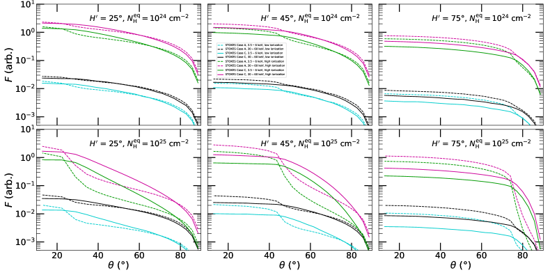
Figure 4.4: Case A (dashed lines) compared to Case C (solid lines): we show the energy-integrated flux, $F$, versus inclination, $\theta$, for $H^{\prime}=25\mbox{${}^{\circ}$}$ (left), $H^{\prime}=45\mbox{${}^{\circ}$}$ (middle), and $H^{\prime}=75\mbox{${}^{\circ}$}$ (right) and for $N_{\textrm{H}}^{\textrm{eq}}=10^{24}\textrm{ cm}^{-2}$ (top) and $N_{\textrm{H}}^{\textrm{eq}}=10^{25}\textrm{ cm}^{-2}$ (bottom). We show the results for low level of ionization, i.e. $\tau_{\textrm{e}}^{\textrm{eq}}=0.007$ for $N_{\textrm{H}}^{\textrm{eq}}=10^{24}\textrm{ cm}^{-2}$ and $\tau_{\textrm{e}}^{\textrm{eq}}=0.07$ for $N_{\textrm{H}}^{\textrm{eq}}=10^{25}\textrm{ cm}^{-2}$, integrated in 3.5–6 keV (blue) and 30–60 keV (black), as well as for high level of ionization, i.e. $\tau_{\textrm{e}}^{\textrm{eq}}=0.7$ for $N_{\textrm{H}}^{\textrm{eq}}=10^{24}\textrm{ cm}^{-2}$ and $\tau_{\textrm{e}}^{\textrm{eq}}=7$ for $N_{\textrm{H}}^{\textrm{eq}}=10^{25}\textrm{ cm}^{-2}$, integrated in 3.5–6 keV (green) and 30–60 keV (magenta). The remaining parameters are $r_{\textrm{in}}^{\textrm{torus}}=0.05$ (Case A), $r_{\textrm{out}}^{\textrm{torus}}=10$ (Case A) and the primary input was set to $\Gamma=2$ and $p_{0}=2\%$ for all displayed cases. Image adapted from Podgorný et al. (2023c).

Figure 4.5 shows the corresponding polarisation state versus inclination for various half-opening angles. The same from a different perspective, i.e. for polarisation versus the half-opening angle for various inclinations is shown in Figure A.27. From these figures, we see with more clarity how the density (causing reprocessing in different volumes) drives the competition between the two orthogonal configurations linked to the mirror symmetry and to the dominant scattering events that occur rather in the equatorial plane, or rather in the meridional plane. The tested lower densities provide almost exclusively parallel polarisation, reaching $\approx 20\%$ in the most suitable geometries, which are typically high inclinations and high half-opening angles. At extremely high $H^{\prime}$, we observe a peak in inclination and a truly equatorial observer would see again slightly less polarized emission than a slightly lower inclined one. For low half-opening angles, the perpendicular polarisation can reach $\approx 25\%$, again non-monotonically with inclination and depending on other parameters. In this regime, there is depolarisation with lower densities, as the photons scatter in large volumes of the equatorial medium, thus on average through higher diversity of directions. For high enough densities, the “periscope” polarisation induction by reflection on the inner walls is stronger for higher ionization of the medium, as it then strongly reflects in the meridional plane for rather low half-opening angles compared to contributions from other scattering directions. Some dependency of polarisation on energy is observed due to the energy-dependent contribution of absorption and the aforementioned two dominant regimes. A wedge-shaped torus is more likely to produce higher parallel oriented polarisation (or less polarized perpendicular polarisation) than a circular torus. The equatorial inner toroidal radius is held the same for both configurations, so the difference is the convexity or concavity of the inner wall in this case, which is critical for first-order scatterings.

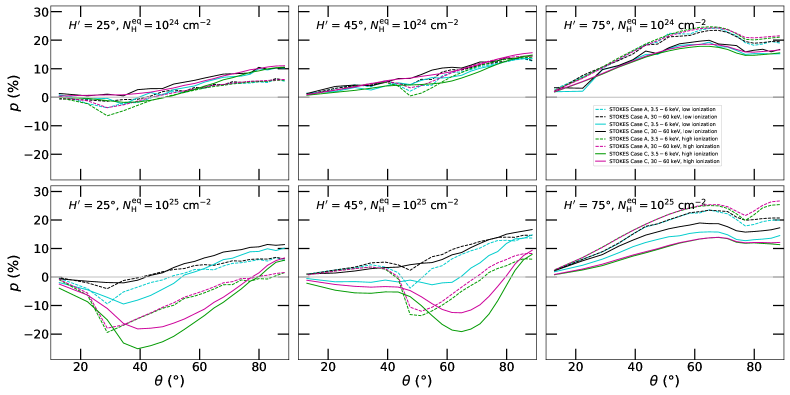
Figure 4.5: The same as in Figure 4.4, but energy-averaged polarisation degree, $p$, versus inclination $\theta$ is shown. Image adapted from Podgorný et al. (2023c).

The switch in polarisation angle and non-monotonic polarisation degree with inclination were also reported for similar investigations in the optical and UV bands (Goosmann and Gaskell, 2007; Marin et al., 2012), as these are mostly geometrical effects, rather independent of the energy band. For a type-2 observer, we obtained almost no difference in the results, if zero-scattered photons were added (see Chapter 5). The results are then similar, although not equivalent, to the X-ray polarisation estimates provided for obscuration models in Ghisellini et al. (1994); Goosmann and Matt (2011); Ratheesh et al. (2021); Ursini et al. (2023b); Veledina et al. (2023b); Tanimoto et al. (2023); Tomaru et al. (2024). In Chapter 5, we will provide perhaps a more comparable view to some of these studies. In particular, the work of Goosmann and Matt (2011) used the same code as us, but the exact modeling conditions were different and the study was targeting particularly the AGN in NGC 1068. Here we aim to provide a much broader overview of the configuration space and to show the striking diversity of possible results for a general source.

We will now turn attention to the effects of changing eccentricity of the elliptical tori. In the same plotting style, we compare in Figures 4.6, 4.7, A.28, A.29 the polarisation versus inclination and half-opening angle for the same two different densities, the same two energy bands and the high level of ionization. We fix $r_{\textrm{in}}^{\textrm{torus}}$ and vary $R^{\prime}$, thus we track the effects of compactness of the entire reprocessing structure with fixed distance to the source. Case C is also plotted over a range of prolate and oblate Cases B, but it does not always represent an!intermediate case due to the adopted definitions (see above). The more oblate the torus is, i.e. equatorially elongated, the more parallel oriented polarisation it produces. In this sense, the most oblate Cases B with $b^{\prime}=3R^{\prime}/4$ provide results closest to the previously shown wedge-shaped Case A, as there are high column density conditions for light rays that pass under inclinations near the half-opening angle. The dependency on eccentricity is reversed only for low half-opening angles, particularly for soft energies, high densities and high inclinations, i.e. when the absorption effects cause preferentially perpendicular polarisation orientation for more oblate tori under extreme obscuration (with low numerical noise seen e.g. in top-middle panel of Figure 4.7 and in comparison with Case A in dashed green curve of bottom-middle panel of Figure 4.5). In this part of the configuration space, the curvature sign (whether convex or concave with respect to the central emission point) of the inner reflecting surface plays larger role. The studies of Ghisellini et al. (1994); Ratheesh et al. (2021); Ursini et al. (2023b); Veledina et al. (2023b) used a conical shape of the obscurer. Although detailed comparisons are beyond the scope of our work, we anticipate the the geometry adopted therein with essentially no inner wall would vary from the elliptical tori presented here most clearly in this corner of the parameter space, perhaps even more from the wedge-shaped Case A torus.

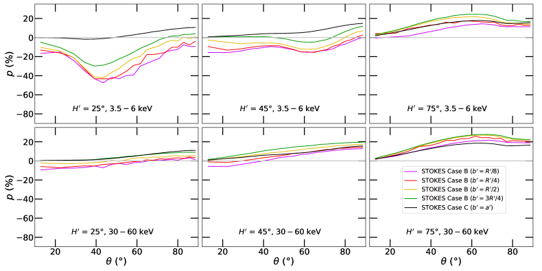
Figure 4.6: Case B for various ellipse eccentricities compared to the circular Case C in energy-averaged polarisation degree, $p$, versus inclination $\theta$ for $H^{\prime}=25\mbox{${}^{\circ}$}$ (left), $H^{\prime}=45\mbox{${}^{\circ}$}$ (middle), and $H^{\prime}=75\mbox{${}^{\circ}$}$ (right). We show the results integrated in 3.5–6 keV (top) and 30–60 keV (bottom) and for $N_{\mathrm{H}}^{\textrm{eq}}=10^{24}\textrm{ cm}^{-2}$. The black curve corresponds to the Case C ($b^{\prime}=a^{\prime}$). The magenta, red, yellow, green curves correspond to the Case B for $b^{\prime}=R^{\prime}/8$, $b^{\prime}=R^{\prime}/4$, $b^{\prime}=R^{\prime}/2$, $b^{\prime}=3R^{\prime}/4$, respectively. The results are shown for high level of ionization, i.e. $\tau_{\textrm{e}}^{\textrm{eq}}=0.7$, see corresponding Figure A.30 for low ionization. The primary input was set to $\Gamma=2$ and $p_{0}=2\%$ for all displayed cases. Image adapted from Podgorný et al. (2023c).

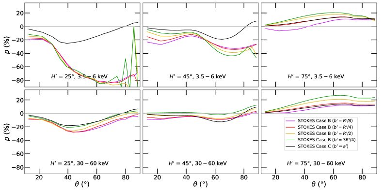
Figure 4.7: The same as in Figure 4.6, but for $N_{\mathrm{H}}^{\textrm{eq}}=10^{25}\textrm{ cm}^{-2}$. The results are shown for high level of ionization, i.e. $\tau_{\textrm{e}}^{\textrm{eq}}=7$, see corresponding Figure A.31 for low ionization. Image adapted from Podgorný et al. (2023c).

The same dependencies of polarisation on inclination are also provided in Figures A.30 and A.31, but for low ionization. Despite more numerical noise being present, because more radiation is absorbed for the same number of simulated photons, we obtained qualitatively the same polarisation response to changing geometry. The results are even quantitatively similar for lower densities, but for higher densities the dispersion in polarisation with respect to the range of eccentricities is smaller in the parallel oriented regime. The reason is the absorption on atoms under these density conditions, which is large enough even for the most prolate cases, compared to pure reflection on free electrons. The furthermost side of the torus with respect to the observer is then unable to produce enough perpendicularly polarized photons to significantly depolarize the parallelly polarized component. In the follow-up section, we will provide a comparison of different ionization cases of the presented MC model within one figure when compared to a different model.

Lastly, we discuss the effects of changing primary radiation. Figure 4.8 shows the polarisation results in the same plotting style for a range in $\Gamma$ and different primary polarisation state, all for Case C and high ionization of the equatorial reprocessing region. Because we do not include direct radiation, the incident polarisation state changing by $2\%$ in polarisation fraction impacts the resulting polarisation by $\lessapprox 2\%$ for a generally inclined observer. The result is depolarized or additionally polarized with respect to the case with unpolarized primary, following the incident polarisation orientation with respect to the polarisation angle for unpolarized primary. The change in photon index $\Gamma$ plays a much larger role, also depolarizing or additionally polarizing with respect to the intermediate $\Gamma=2$ example. The change in net polarisation with respect to the unpolarized primary or $\Gamma=2$ case is qualitatively in the same direction in the plots, when the polarisation fraction passes the zero point and the polarisation angle switches, which again suggests two competing directions of polarisation generation. We omit the discussion of spectral lines, where the equivalent width would be also $\Gamma$-dependent. The energy dependence of polarisation, which is geometry and density dependent (see Figure 4.3), plays a role while $\Gamma$ influences the relative importance of soft and hard X-rays. We simply weight more over higher or lower polarised energy bins, when changing $\Gamma$ and plotting the energy-integrated results. The difference can be even as large as $\approx 20\%$ in 3.5–6 keV polarisation for the demonstrated large change in photon index for high column densities. In Chapter 5, we will evaluate the degeneracy in the results for a single 2–8 keV polarimetric observation by IXPE. When testing other ionization levels in the obscuring media, the dispersion in polarisation with respect to the changing properties of primary radiation appears similar. It varies, however, with chosen geometry. The displayed Case C represents an intermediate result. The more prolate elliptical tori are more sensitive to the change of $\Gamma$ (up to $30\%$ difference in polarisation in the most critical configurations in 3.5–6 keV), while the more oblate elliptical tori and wedge-shaped tori show minor changes (maximum of $10\%$ difference in polarisation in the most sensitive configurations in 3.5–6 keV).

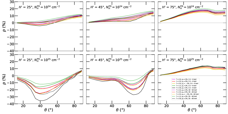
Figure 4.8: Case C only for different cases of primary radiation: energy-averaged polarisation degree, $p$, versus inclination $\theta$ for $H^{\prime}=25\mbox{${}^{\circ}$}$ (left), $H^{\prime}=45\mbox{${}^{\circ}$}$ (middle), and $H^{\prime}=75\mbox{${}^{\circ}$}$ (right). We show the results integrated in 3.5–6 keV (solid) and 30–60 keV (dashed) and for $N_{\mathrm{H}}^{\textrm{eq}}=10^{24}\textrm{ cm}^{-2}$ and $\tau_{\textrm{e}}^{\textrm{eq}}=0.7$ (top) and $N_{\mathrm{H}}^{\textrm{eq}}=10^{25}\textrm{ cm}^{-2}$ and $\tau_{\textrm{e}}^{\textrm{eq}}=7$ (bottom). The magenta curves correspond to the $2\%$ parallelly polarized primary with $\Gamma=2.0$. The red and yellow correspond to the unpolarized and $2\%$ perpendicularly polarized primary with $\Gamma=2.0$, respectively. The green and black curves correspond to the $2\%$ parallelly polarized primary with $\Gamma=1.2$ and $\Gamma=2.8$, respectively. The results are shown for high ionization, although other ionization levels show similar dispersion in polarisation with respect to the changing primary input. This dispersion is different with respect to the chosen geometry, while the displayed Case C represents an intermediate result from all tested cases. Image adapted from Podgorný et al. (2023c).

We do not aim to study the imprints of extended or unisotropic sources. Any such consideration would require a separate model design. Perhaps even more useful configuration that we do not consider is thermal emission (or combined thermal and power-law emission) from the central disc-corona region, appearing in the soft state of XRBs, which may be also physically covered in highly obscuring equatorial outflows. Because we obtained different results for different slope of the primary power-law, we expect that adding a strong thermal radiation would affect the results in a way that increasing $\Gamma$ does. The change in spectral shape should play a larger role than any changed primary polarisation of such spectral state (in fact, the first IXPE results do not reveal a significant change in polarisation for XRB spectral changes, Rodriguez Cavero et al., 2023; Ingram et al., 2023a, Steiner et al., in prep.). We refer to the study of Tomaru et al. (2024) that obtained parallelly polarized results from scattering of thermal emission in optically thin winds.

4.2 Simple models of axially symmetric
reflecting structures

In this section, we first explore a simplified model of reflection off the inner walls of a geometrical torus, using the same isotropically emitted power-law, originating in the center of coordinates with a prescribed incident polarisation state. We still do not account for any direct radiation. By “reflection” we mean reprocessing, as usual, because we will use the spectropolarimetric local reflection tables, described in Section 2.1 (in the version published in Podgorný et al., 2022), integrated over the torus surface. However, only a “single-reprocessing” mode is allowed, meaning that the photons can enter and escape the scattering region only once. Because the local reflection model was developed for accretion discs’s atmospheres, we will use only the most neutral part of the tables, i.e. the lowest $\xi$ available, to represent the cold parsec-scale dusty tori of AGNs. The torus has a circular profile (Case C in Section 4.1), is fully opaque, and we consider only illumination of the upper half-space, as if there was an absorbing optically thick material extending from the outer disc to the inner torus boundary. Figure 4.10 shows the model parametrization. An observer can be inclined at any angle $0\mbox{${}^{\circ}$}<\theta<90\mbox{${}^{\circ}$}$ and the torus is assumed to have again some half-opening angle $H^{\prime}$. The inner surface of the torus is illuminated from the equatorial plane up to its shadow boundary, given by the half-opening angle. The observer’s inclination then additionally constrains an area that is the intersection of the visible surface and the illuminated surface that we account for. These are marked in Figure 4.10 as orange-shaded and pink-shaded regions for a generic type-1 ($\theta<H^{\prime}$) and type-2 ($\theta>H^{\prime}$) observer, respectively. In this setup, we may directly compare the results to the MC modeling for Case C, described in Section 4.1. We can then assess to what extent the X-ray polarisation is given solely by the geometrical parameters $\theta$ and $H^{\prime}$ and by single reprocessing, in contrast to self-irradiation and partial transparency effects allowed in the MC modeling.

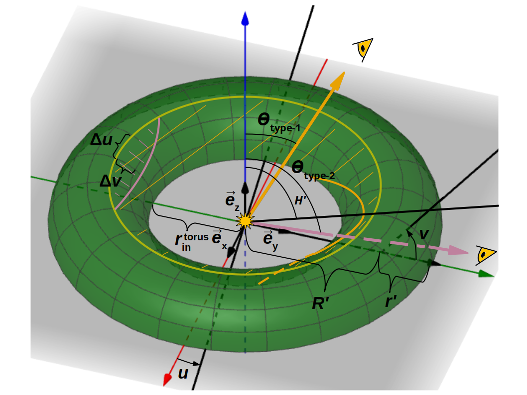
Figure 4.9: A circular toroidal reflector that is considered for the results presented in Section 4.2.1. Being located in the center of the coordinate system, the X-ray power-law of arbitrary incident polarisation and power-law index $\Gamma$ is isotropically illuminating the inner side of the torus surface. We neglect the half-space below the equator, as if there was fully absorbing material in the equatorial plane. The observer, generally inclined at $0\mbox{${}^{\circ}$}<i<90\mbox{${}^{\circ}$}$, is viewing the source in the $yz$-plane. The material only reflects once by means of local reprocessings, i.e. the photons emerge from the same macroscopic location, as they hit. The surface regions not directly illuminated by the central source are not accounted for, i.e. the $v$ values lower than reaching the tangent points of the torus with the half-opening angle cone that are represented by the yellow shadow boundary. The illuminated part cannot be in addition self-obscured by the torus in the observer’s line of sight to be accounted for in the integration. The lower boundaries of the areas that are obscured by the opaque torus for an observer in two generic $\theta_{\textrm{type-1}}$ and $\theta_{\textrm{type-2}}$ inclinations are schematically drawn in orange and pink colors, respectively. The visible reflecting areas for a generic type-1 and type-2 observer are then shaded in orange and pink, respectively. Image adapted from Podgorný et al. (2023b).

Figure 4.10: The energy-dependent results from the xsstokes_torus model. Top: the spectra, $EF_{\mathrm{E}}$, normalized to value at 50 keV. Bottom: the corresponding polarisation degree, $p$, versus energy. For easy comparisons, we show the xsstokes_torus results in the same way as the results from pure MC simulations are given in Figure 4.3. Various inclinations $\theta$ and half-opening angles $H^{\prime}$ for both type-1 and type-2 observers are shown in the color code. The primary input was set to $\Gamma=2$ and $p_{0}=2\%$ for all displayed cases. The highest discrepancies between the pure MC model and the simplistic scenario occurs for high inclinations and high half-opening angles. The curvature and relative size effects of the torus surface are eliminated from such comparisons, because the torus in both models (Case C) has identical profile. The detailed parametric dependencies are shown in the following figures when integrated in energy. Image adapted from Podgorný et al. (2023b).

The numerical implementation is in detail described in Appendix D, as the calculation was divided in three steps, each comprising of a newly developed routine that can be of wider use. The final model, called xsstokes, is compatible with XSPEC and efficiently interpolates for arbitrary state of primary polarisation, using equation

$$\begin{split}S(p_{0},\Psi_{0})=&\,S(0,-)+p_{0}\Big{\{}\left[S(0,-)-S\left(1,\frac{\pi}{2}\right)\right]\cos{2(\Psi_{0})}\\ &\quad+\left[S\left(1,\frac{\pi}{4}\right)-S(0,-)\right]\sin{2(\Psi_{0})}\Big{\}}\,,\end{split}$$ (4.3)

which is just a variant of (3.1) that was used for the same problem in Chapter 3, but could not be used here, as we work with the older version of local reflection tables, pre-computed for unpolarized, $100\%$ diagonally polarized and $100\%$ horizontally polarized emission. The same interpolation scheme works for any axially symmetric reflector. Thus, in this variant of an equatorial toroidal obscuring medium, we use a subversion name xsstokes_torus. But we also modelled one other reflection scenario imitating a faraway disc in the equatorial plane, which in the exact same way interpolates for arbitrary incident polarisation.

This effort resulted in another XSPEC compatible model, a subvariant of xsstokes, called xsstokes_disc. It represents the same nearly neutral local reflection tables from Podgorný et al. (2022) integrated uniformly, i.e. with no weighting applied, in all azimuthal emission angles $\Phi_{\textrm{e}}$ and in a range of high incident inclination angles: $0\leq\mu_{\textrm{i}}\leq M_{\mathrm{i}}$, where $M_{\mathrm{i}}=0.3$. Such model illustrates a distant region of the accretion disc, illuminated by a central vertically extended hot inner-accretion flow of Comptonized emission and/or a reflecting outer accretion disc with increasing geometrical thickness. We note, however, that the latter geometrical imagination results in a range of surface emission inclination angles for a particular distant observer, if the reflecting medium deviates from the equatorial plane non-linearly, while we keep a particular emission angle $\theta$ (adopted as $\delta_{\textrm{e}}$ from the original tables) as a free parameter, which drives the polarisation results to a significant extent. We assume the disc to be truncated (or supported in XSPEC by a different reflection model in the inner hot parts) and the inner-accreting system to be unobscured even for large inclination angles. The results of the xsstokes_disc model are presented here below, in comparison to the corresponding limiting case of a torus with high half-opening angle.

All results presented in this section and in Appendix D are part of Podgorný et al. (2023b), which is, however, still under review process. Therefore, we present these results as preliminary and note that the model will still undergo many changes in the near future. For example, the parameter $M_{\mathrm{i}}$ is being currently implemented as a model parameter, representing the coronal physical size (large $M_{\mathrm{i}}$ is equivalent to the KYNSTOKES results in sandwich geometry without kinetic and relativistic effects). For the reflection on a torus, we plan to add a new parameter $B=\{0,1\}$, representing a switch between taking the reflecting area below the torus equator into account or not. Another pending issue is the fact that for every half-opening angle there is an inclination above which the observer does not see any illuminated surface area on the torus. This is important for small half-opening angles and the $H^{\prime}$ parameter should be thus transformed to range between 0 and 1, effectively spanning all allowed values per inclination $\theta$, in order to not be able to fit in XSPEC at higher inclinations.

For all results presented in this section, we keep the notation of a positive and negative polarisation degree for parallel or perpendicular polarisation orientation of the incident or emergent radiation, respectively. No other polarisation angle cases are considered on the input and no relativistic effects are considered inside the simulations that would result in symmetry breaking.

4.2.1 Reflection from inner walls of a geometrical torus

Let us first discuss the results of the xsstokes_torus model. Figure 4.10 shows the energy-dependent spectra and polarisation for a selection of $\theta$ and $H^{\prime}$, displayed in the same way as in Figure 4.3. Compared to the MC simulations presented in Section 4.1, we obtain much lower numerical noise and generally higher predicted polarisation fraction in the perpendicular orientation, while qualitative behavior of the polarisation degree and angle with $\theta$ and $H^{\prime}$ is similar. The depolarisation in spectral lines is preserved. From the spectra it is clear that even the most neutral part of the local reflection tables does not allow strong absorption towards the soft X-rays and the associated continuum polarisation fraction is rather constant in energy in 1–4 keV. We obtain closer results to the elliptical tori class (Cases B and C) presented in Section 4.1 than to the wedge-shaped tori (Case A) from Section 4.1. The case of the highest inclination and the smallest half-opening angle scenario from Figure 4.3 is not shown, because in xsstokes_torus we have the zero-transparency condition and the reflecting area is already eclipsed in such case.

Figure 4.11 and A.32 show the polarisation results versus inclination and half-opening angle, respectively, integrated in the 3.5–6 keV and 30–60 keV bands that are not contaminated by spectral lines. On these figures, we compare directly the X-ray polarisation from xsstokes_torus with the MC modeling results from Section 4.1 for various ionization levels and equatorial column densities. Albeit they both show the same data from a different perspective, these two figures are additionally illustrative, because we did not compare different ionization levels of the MC model in Section 4.1 in the same panels. We cut the xsstokes_torus parameter space for low half-opening angles and high inclinations, where the illuminated area is fully obscured. It is clear from these figures that the highest polarisation contribution from the perpendicularly polarized component arises from the torus with highest free electron density contribution alongside high neutral hydrogen density (low transparency conditions). This is also the case that resembles most the xsstokes_torus model, which takes into account only the highly reflective and perpendicularly polarized component originating on the furthermost side of the inner walls of the torus from the observer. The xsstokes_torus model results in about twice higher polarisation fraction for low and moderate half-opening angles. It also predicts parallelly oriented net polarisation for high half-opening angles, but then the resulting polarisation fraction is on the contrary about twice lower than for the pure MC model due to the lack of strong flux contribution of the parallelly polarized component, originating in reflection from left and right sides of the torus inner walls from the observer’s perspective. In the MC simulations, the parallelly polarized component is strengthened by means of partial transparency.

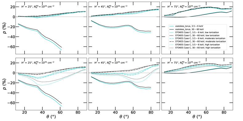
Figure 4.11: Comparison of the pure STOKES simulation of Case C from Section 4.1 (with different line styles assigned to different ionization levels) with the xsstokes_torus results (solid). We plot the polarisation degree, $p$, versus inclination $\theta$ for $H^{\prime}=25\mbox{${}^{\circ}$}$ (left), $H^{\prime}=45\mbox{${}^{\circ}$}$ (middle), and $H^{\prime}=75\mbox{${}^{\circ}$}$ (right). We show the results integrated in 3.5–6 keV (blue) and 30–60 keV (black) and for $N_{\textrm{H}}^{\textrm{eq}}=10^{24}\textrm{ cm}^{-2}$ in STOKES Case C (top) and $N_{\textrm{H}}^{\textrm{eq}}=10^{25}\textrm{ cm}^{-2}$ in STOKES Case C (bottom). The primary input was set to $\Gamma=2$ and $p_{0}=2\%$ for all displayed cases. Image adapted from Podgorný et al. (2023b).

4.2.2 Reflection from a faraway disc

We now return to the problem of disc reflection with no SR or GR effects applied, as computed by the xsstokes_disc model. Figure 4.12 shows the polarisation dependence on energy for various observer’s inclinations, primary power-law indices and primary polarisation states. Unlike the result for reflection from a toroidal structure that has non-negligible vertical extension from the equatorial plane, here we obtain only parallel polarisation angle on the output. This is natural regarding polarisation arising from Compton scattering (see Section 1.1.2) in no distortion of space-time geometry, when the source of illumination is located in the center of the system and the scattering plane is rather aligned with the matter distribution. Nearly the same orientation of polarisation by disc reflection was obtained also in the lamp-post geometries with KYNSTOKES in Section 3.1.1, where the disc was reaching to the ISCO and GR effects were included. The received polarisation fraction by disc reflection in xsstokes_disc can be any value between $0\%$ up to $\approx 30\%$, strongly depending on the inclination of the observer, which is the main driver of polarisation here. The spectral lines are again depolarized, as evident from the local disc reflection tables. The energy profile of polarisation degree agrees with that of the xsstokes_torus model, seen in Figure 4.10, that uses the same local reflection tables.

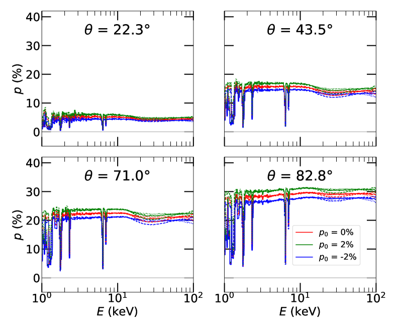
Figure 4.12: The polarisation degree, $p$, versus energy for distant disc reflection computed by xsstokes_disc. We show the results for various cosines of the observer’s inclination: $\mu_{\textrm{e}}=0.925$ (top left panel), $\mu_{\textrm{e}}=0.725$ (top right panel), $\mu_{\textrm{e}}=0.525$ (bottom left panel), $\mu_{\textrm{e}}=0.125$ (bottom right panel). The color code represents different incident polarisations of the primary power-law: unpolarized (red), $2\%$ parallelly polarized (green), and $2\%$ perpendicularly polarized (blue). The solid lines correspond to $\Gamma=2.0$, dashed lines to $\Gamma=1.2$, dotted lines to $\Gamma=2.8$. Image adapted from Podgorný et al. (2023b).

What varies from the torus reflection is the impact of changing primary power-law index on the emergent polarisation, which is negligible in the majority of the parameter space covered by xsstokes_disc (apart from $\approx 2\%$ difference in polarisation around 30 keV for high inclinations). The response of the reflected polarisation degree to the incident polarisation is “linear” in the same sense as for the KYNSTOKES results presented in Section 3.1.1 or as for the reflection from a geometrical torus described above. The received emission has enhanced polarisation compared to unpolarized primary case by less or the same percentage of the incident polarisation fraction, if the incident polarisation is oriented parallelly, and is depolarized compared to unpolarized primary case by less or the same percentage, if the incident polarisation is oriented perpendicularly. These effects are nearly energy-independent.

To study the inclination dependence in more detail, we again integrate the polarisation results in the 3.5–6 keV and 30–60 keV bands, which is shown in Figure 4.14 for one chosen $\Gamma$. We obtain here a monotonic and roughly linear dependency of polarisation degree on observer’s inclination. This is a consistent limit of the torus reflection models for high half-opening angles (see e.g. Figure 4.11, right panels), similarly to the net polarisation angle results. Due to effectively higher asymmetry in the geometry of scattering for the truncated disc reflection, we obtain higher polarisation fraction than with the torus reflection models where we operate with more competing scattering directions with respect to the observer. The xsstokes_disc results displayed in Figure 4.14 are in line with figure 11 from Ratheesh et al. (2021), which solved for a similar equatorial disc reflection problem with codes from Matt et al. (1989, 1991). Although the dependency on inclination is consistent between the two figures, Ratheesh et al. (2021) obtained about twice lower resulting polarisation, likely because they solved for more isotropic illumination of the disc. Our mitigation of the incident angles to $0\leq\mu_{\textrm{i}}\leq 0.3$ then again reduces the allowed scattering plane directions. The inclination dependence of polarisation obtained in our model is also consistent with the results predicted by single-scattering Chandrasekhar’s approximation for reflection (1.39), integrated in $\mu_{\textrm{i}}$ and $\Phi_{\textrm{e}}$ accordingly, which is shown in Figure 4.14. The fact that the absolute values of polarisation degree and angle are matching too is natural, as for nearly neutral media we expect results closer to the single-scattering results, while highly ionized reflection should rather be approximated by the diffuse Chandrasekhar’s approximation.

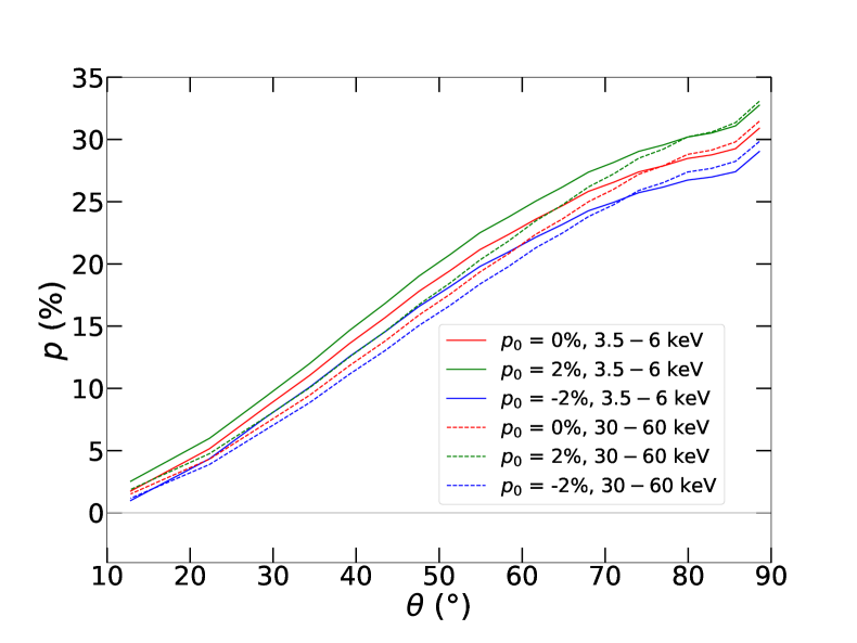
Figure 4.13: The computed energy-averaged polarisation fraction, $p$, with xsstokes_disc in 3.5–6 keV (solid lines) and 30–60 keV (dashed lines) versus observer’s inclination $\theta$ for $\Gamma=2$. The color code represents different incident polarisations of the primary power-law: unpolarized (red), $2\%$ parallelly polarized (green), and $2\%$ perpendicularly polarized (blue). Image adapted from Podgorný et al. (2023b).

Figure 4.14: The absolute value of polarisation, $\lvert p\rvert$, versus observer’s inclination $\theta$. The results are from Chandrasekhar’s single-scattering approximation (1.39) integrated uniformly in all azimuthal emission angles $\Phi_{\textrm{e}}$ and in selected ranges of cosines of incident angles $0\leq\mu_{\textrm{i}}\leq 0.3$ (solid lines), $0\leq\mu_{\textrm{i}}\leq 0.8$ (dashed lines) and $0\leq\mu_{\textrm{i}}\leq 1$ (dotted lines). The color code represents different incident polarisation states of the primary, unpolarized and $2\%$ parallelly and perpendicularly polarized. Image adapted from Podgorný et al. (2023b).

We add two other cases of integration ranges of the incident angles for Chandrasekhar’s single-scattering approximation in Figure 4.14. The unpolarized result is not achieved for fully isotropic irradiation, but rather for $0\leq\mu_{\textrm{i}}\lessapprox 0.8$. If we continue to increase the range of illumination angles beyond this range up to $0\leq\mu_{\textrm{i}}\leq 1$, the resulting polarisation switches orientation to become parallel with the disc, as the rays arriving at the disc in vertical direction begin to dominate the polarisation output. We thus display the absolute value of polarisation, $\lvert p\rvert$, to directly compare the obtained polarisation fraction between the three cases. The fully isotropic irradiation case reaches maximum polarisation fraction at $\approx 20\%$ for edge-on observers, as we mentioned already in Section 1.5.1. The orthogonal net polarisation then causes inverted response of the emergent polarisation degree to the incident polarisation angle. The resulting orientation means that elementary right-angle principles are in play and that the same explanations are behind the dominant polarisation orientation emerging from the relativistic lamp-post and sandwich coronal reflection models discussed in Chapter 3. While the lamp-post, at least for low heights $h$, is rather causing the projected photon paths to be equatorial and results in disc-reflected polarisation angles nearly parallel with the principal axis, the extended slab coronal model presented imposes higher relative contribution of photons emitted vertically towards the disc (the local reflection tables in KYNSTOKES for extended coronae are indeed integrated in the entire range of $0\leq\mu_{\textrm{i}}\leq 1$), which in most cases results in prevailing disc-reflected polarisation angles parallel to the disc.

4.3 Polarized X-ray emission from an entire
active galactic nucleus

Last but not least, we attempted for a toy model of an entire AGN that is schematically shown and parametrized in Figure 4.2. The modeling is described in Podgorný et al. (2024) and summarized here below. We return to the MC simulations of the reprocessings in parsec-scale components of AGNs performed entirely with STOKES v2.07, as in Section 4.1. We now account also for direct emission. We assume a 3-component model consisting of (i) a point source of emission located in the center of coordinates, representing the inner disc-corona system, (ii) a homogeneous wedge-shaped equatorial torus (Case A) discussed in Section 4.1, which is glued at fixed half-opening angle $H^{\prime}=60^{\circ}$ to (iii) two axially symmetric homogeneous polar scattering regions of the same wedge-shaped meridional profile, representing polar winds in form of NLRs. The same model was adopted for type-1 ($\theta=20^{\circ}$) and type-2 ($\theta=70^{\circ}$) AGN studies in Marin et al. (2018a, b). Here we replace the central emission lamp-post model used in Marin et al. (2018a, b) with the KYNSTOKES model from Podgorný et al. (2023a) in the lamp-post regime. The difference from Marin et al. (2018a, b) in the central illumination is the newly computed local disc reflection tables that allow to study partially ionized disc effects and a correction in the polarized GR radiative transfer between the lamp and the disc. We will argue that even a simple 3-component model with circumnuclear components of uniform density and one geometry can produce diverse X-ray polarisation outcome, similarly to the discussion in Section 4.1. General observational prospects for this model with respect to the IXPE and eXTP missions, i.e. without a focus on a particular source, will be given in Chapter 5.

As in Marin et al. (2018a, b), regarding the central emission region we tested the limiting examples of black-hole spins $a=0$ and $a=1$, while examining a nearly neutral disc ($L_{\textrm{X}}/L_{\textrm{Edd}}=0.001$ and $M/M_{\odot}=10^{8}$ in KYNSTOKES, comparable to the neutral disc computations in Marin et al., 2018b, a) and highly ionized disc reflection ($L_{\textrm{X}}/L_{\textrm{Edd}}=0.1$ and $M/M_{\odot}=10^{5}$ in KYNSTOKES). We evaluated the cases of unpolarized and $2\%$ parallelly and perpendicularly polarized primary power-law (with $\Gamma=2$), prescribed at the lamp-post, which are denoted by $p_{0}=0\%$, $p_{0}=2\%$ and $p_{0}=-2\%$. We stress that the lamp-post coronal geometry is a) simplistic and b) not supported by the recent IXPE discoveries (see Chapter 5). However, it is in line with one-to-one comparisons to Marin et al. (2018a, b) and by assessing different polarisation angles, we may also mimic different coronal geometries. Investigation of the impact of coronae with non-negligible size with respect to the distant components or of any sort of thermal radiation in the X-rays is exceeding the extent of this work.

In the same way as in Marin et al. (2018a, b), we consider semi-isotropic illumination of the parsec-scale scattering regions, i.e. the polar winds are illuminated by the KYNSTOKES output for $\theta=20^{\circ}$ and the equatorial regions by the KYNSTOKES output for $\theta=70^{\circ}$. Relativistic effects are neglected in the subsequent MC simulation that models only the reprocessing in the distant equatorial and polar components, which happens simultaneously (one photon can escape and reach any scattering region at any time during its journey). The faraway scatterers are considered cold, as they do not thermally radiate, but we again treat the partial ionization of these regions simplistically by means of free uniform density of electrons $n_{\textrm{e}}$. We consider different values neutral hydrogen column densities of the torus and polar winds, denoted by $N_{\textrm{H}}^{\textrm{eq}}=n_{\textrm{H}}(r_{\textrm{out}}^{\textrm{torus}}-r_{\textrm{in}}^{\textrm{torus}})$ and $N_{\textrm{H}}^{\textrm{wind}}=n_{\textrm{H}}(r_{\textrm{out}}^{\textrm{wind}}-r_{\textrm{in}}^{\textrm{wind}})$, respectively. We use again the solar abundance from Asplund et al. (2005) with $A_{\mathrm{Fe}}=1.0$. For type-2 viewing angles of AGNs, in addition to the absorbing polar winds, the cases of ionized polar winds and no polar winds are considered, as in Marin et al. (2018b). Direct comparisons with previous studies are the main reason for the configurations adopted. The neutral polar winds are less physical, but could be an illustrative example in the spirit of aspiring to understand what inside the system causes what on the output and which processes are negligible compared to others. We refer to Tables 4.1 and 4.2 that summarize the model grid for type-1 and type-2 AGNs, respectively, and introduce the 2–8 keV average polarisation results (in positive and negative polarisation convention), as well as observational prospects that will be elaborated on in Chapter 5. We refer to Marin et al. (2018a, b) for details on the parameter space explored that is physically and observationally motivated and that we fully adopt here, because the principal aim is to track to what extent the change in inner emission region plays a role. We will show, however, that other (unexpected) discrepancies from Marin et al. (2018a, b) were also identified with the latest simulations.

Table 4.1: The main configuration space for type-1 AGNs. In addition to those parameters studied in Marin et al. (2018a, b), the effect of partial disc ionization was tested with KYNSTOKES. The column densities $N_{\textrm{H}}^{\textrm{eq}}$ and $N_{\textrm{H}}^{\textrm{wind}}$ are provided in $\textrm{cm}^{-2}$. Top value in each slot (black bold) is the model unfolded 2–8 keV average polarisation degree, $p$, for a given configuration. The rest of the table will be discussed in Chapter 5. The three values in the left column in each slot (blue) are the estimated observational times, $T_{\textrm{obs}}\,[\textrm{Ms}]$, that are required for the model $|p|$ to exceed the simulated $M\!D\!P_{99\%}$ for IXPE (evaluates whether the polarisation is to be detected at a $99\%$ confidence level, although here we compare only the unfolded model), using the unweighted approach in IXPEOBSSIM, if the observed X-ray flux is $F_{\mathrm{X,2-10}}=1\times 10^{-10},5\times 10^{-11},1\times 10^{-11}\,\textrm{erg cm}^{-2}\,\textrm{s}^{-1}$ from top to bottom, respectively, and that were linearly interpolated in the computed $\{T_{\textrm{obs}},F_{\textrm{X,2-10}}\}$ space. The three values in the right column in each slot (red) are the estimated observed X-ray fluxes, $F_{\mathrm{X,2-10}}\,[10^{-10}\,\textrm{erg cm}^{-2}\,\textrm{s}^{-1}]$, that are required for the model $|p|$ to exceed the simulated $M\!D\!P_{99\%}$, using the unweighted approach in IXPEOBSSIM, if the observational time is $T_{\mathrm{obs}}=0.5,1,1.5\,\textrm{Ms}$ from top to bottom, respectively, and that were linearly interpolated in the computed $\{T_{\textrm{obs}},F_{\textrm{X,2-10}}\}$ space. The results are serving as first-order estimates only, see Chapter 5 for details. For a particular source, more specific information on its composition may be obtained, which enables detectability predictions with higher accuracy. The $M\!D\!P_{99\%}$ values can be also slightly reduced by means of weighted approach in IXPEOBSSIM, which is available for real data analysis with IXPE (Di Marco et al., 2022). The observational times needed for IXPE may be reduced by about a factor of 4 for eXTP due to its larger effective mirror area and other instrumental differences.

			type-1 AGNs (absorbing winds only)
			$N_{\textrm{H}}^{\textrm{wind}}=10^{21}$						$N_{\textrm{H}}^{\textrm{wind}}=10^{22}$		$N_{\textrm{H}}^{\textrm{wind}}=10^{23}$
			$N_{\textrm{H}}^{\textrm{eq}}=10^{23}$		$N_{\textrm{H}}^{\textrm{eq}}=10^{24}$		$N_{\textrm{H}}^{\textrm{eq}}=10^{25}$		$N_{\textrm{H}}^{\textrm{eq}}=10^{24}$		$N_{\textrm{H}}^{\textrm{eq}}=10^{24}$
					$p$ = 0.3 %
					$>$9.9	$>$5.30
					$>$9.9	$>$5.30
		$a=0$			$>$9.9	$>$5.30
					$p$ = 0.4 %
					$>$9.9	$>$5.30
					$>$9.9	$>$5.30
	$p_{0}=0\%$	$a=1$			$>$9.9	$>$5.30
			$p$ = 2.0 %		$p$ = 2.0 %		$p$ = 2.0 %		$p$ = 2.0 %		$p$ = 2.1 %
			$>$9.9	$>$5.30	$>$9.9	$>$5.30	$>$9.9	$>$5.30	$>$9.9	$>$5.30	$>$9.9	$>$5.30
			$>$9.9	5.01	$>$9.9	5.06	$>$9.9	4.95	$>$9.9	4.93	$>$9.9	$>$5.30
		$a=0$	$>$9.9	4.05	$>$9.9	4.11	$>$9.9	3.99	$>$9.9	3.96	$>$9.9	4.93
			$p$ = 1.9 %		$p$ = 2.0 %		$p$ = 2.0 %		$p$ = 2.0 %		$p$ = 2.0 %
			$>$9.9	$>$5.30	$>$9.9	$>$5.30	$>$9.9	$>$5.30	$>$9.9	$>$5.30	$>$9.9	$>$5.30
			$>$9.9	$>$5.30	$>$9.9	$>$5.30	$>$9.9	5.29	$>$9.9	5.29	$>$9.9	$>$5.30
	$p_{0}=2\%$	$a=1$	$>$9.9	4.41	$>$9.9	4.49	$>$9.9	4.39	$>$9.9	4.38	$>$9.9	$>$5.30
					$p$ = -1.4 %
					$>$9.9	$>$5.30
					$>$9.9	$>$5.30
		$a=0$			$>$9.9	$>$5.30
					$p$ = -1.2 %
					$>$9.9	$>$5.30
					$>$9.9	$>$5.30
neutral disc	$p_{0}=-2\%$	$a=1$			$>$9.9	$>$5.30
					$p$ = 0.5 %
					$>$9.9	$>$5.30
					$>$9.9	$>$5.30
		$a=0$			$>$9.9	$>$5.30
					$p$ = 0.7 %
					$>$9.9	$>$5.30
					$>$9.9	$>$5.30
	$p_{0}=0\%$	$a=1$			$>$9.9	$>$5.30
			$p$ = 2.0 %		$p$ = 2.0 %		$p$ = 2.0 %		$p$ = 2.0 %		$p$ = 2.1 %
			$>$9.9	$>$5.30	$>$9.9	$>$5.30	$>$9.9	$>$5.30	$>$9.9	$>$5.30	$>$9.9	$>$5.30
			$>$9.9	4.99	$>$9.9	5.11	$>$9.9	5.05	$>$9.9	4.93	$>$9.9	$>$5.30
		$a=0$	$>$9.9	4.03	$>$9.9	4.16	$>$9.9	4.10	$>$9.9	3.96	$>$9.9	4.81
			$p$ = 1.8 %		$p$ = 1.7 %		$p$ = 1.6 %		$p$ = 1.7 %		$p$ = 1.7 %
			$>$9.9	$>$5.30	$>$9.9	$>$5.30	$>$9.9	$>$5.30	$>$9.9	$>$5.30	$>$9.9	$>$5.30
			$>$9.9	$>$5.30	$>$9.9	$>$5.30	$>$9.9	$>$5.30	$>$9.9	$>$5.30	$>$9.9	$>$5.30
	$p_{0}=2\%$	$a=1$	$>$9.9	4.68	$>$9.9	5.05	$>$9.9	5.11	$>$9.9	4.84	$>$9.9	$>$5.30
					$p$ = -1.1 %
					$>$9.9	$>$5.30
					$>$9.9	$>$5.30
		$a=0$			$>$9.9	$>$5.30
					$p$ = -0.3 %
					$>$9.9	$>$5.30
					$>$9.9	$>$5.30
ionized disc	$p_{0}=-2\%$	$a=1$			$>$9.9	$>$5.30

Table 4.2: The same as in Table 4.1, but for the studied type-2 AGNs cases. The tested flux values for interpolation of observational times (in blue from top to bottom in each configuration) are $F_{\mathrm{X,2-10}}=1\times 10^{-11},9\times 10^{-12},8\times 10^{-12}\,\textrm{erg cm}^{-2}\,\textrm{s}^{-1}$.

			type-2 AGNs
			absorbing winds with $N_{\textrm{H}}^{\textrm{wind}}=10^{21}$						ionized winds						no winds
			$N_{\textrm{H}}^{\textrm{eq}}=10^{23}$		$N_{\textrm{H}}^{\textrm{eq}}=10^{24}$		$N_{\textrm{H}}^{\textrm{eq}}=10^{25}$		$N_{\textrm{H}}^{\textrm{eq}}=10^{23}$		$N_{\textrm{H}}^{\textrm{eq}}=10^{24}$		$N_{\textrm{H}}^{\textrm{eq}}=10^{25}$		$N_{\textrm{H}}^{\textrm{eq}}=10^{23}$		$N_{\textrm{H}}^{\textrm{eq}}=10^{24}$		$N_{\textrm{H}}^{\textrm{eq}}=10^{25}$
			$p$ = 6.9 %		$p$ = 1.5 %		$p$ = -19.1 %		$p$ = -0.5 %		$p$ = -18.6 %		$p$ = -26.4 %		$p$ = 7.2 %		$p$ = 3.3 %		$p$ = -0.6 %
			$>$9.9	1.30	$>$9.9	$>$5.30	2.9	0.30	$>$9.9	$>$5.30	3.5	0.33	0.8	0.14	$>$9.9	1.26	$>$9.9	$>$5.30	$>$9.9	$>$5.30
			$>$9.9	0.88	$>$9.9	$>$5.30	3.2	0.19	$>$9.9	$>$5.30	3.8	0.23	0.9	$<$0.08	$>$9.9	0.84	$>$9.9	4.84	$>$9.9	$>$5.30
		$a=0$	$>$9.9	0.64	$>$9.9	$>$5.30	3.4	0.15	$>$9.9	$>$5.30	3.9	0.16	1.0	$<$0.08	$>$9.9	0.62	$>$9.9	3.85	$>$9.9	$>$5.30
			$p$ = 7.2 %		$p$ = 2.0 %		$p$ = -18.3 %		$p$ = -0.3 %		$p$ = -18.1 %		$p$ = -26.2 %		$p$ = 7.4 %		$p$ = 3.7 %		$p$ = -0.4 %
			$>$9.9	1.31	$>$9.9	$>$5.30	3.4	0.33	$>$9.9	$>$5.30	4.0	0.40	1.1	0.16	$>$9.9	1.28	$>$9.9	$>$5.30	$>$9.9	$>$5.30
			$>$9.9	0.89	$>$9.9	$>$5.30	3.6	0.23	$>$9.9	$>$5.30	4.4	0.25	1.3	0.11	$>$9.9	0.85	$>$9.9	4.21	$>$9.9	$>$5.30
	$p_{0}=0\%$	$a=1$	$>$9.9	0.64	$>$9.9	$>$5.30	3.7	0.16	$>$9.9	$>$5.30	4.8	0.19	1.3	$<$0.08	$>$9.9	0.62	$>$9.9	3.11	$>$9.9	$>$5.30
			$p$ = 7.6 %		$p$ = 2.3 %		$p$ = -18.6 %		$p$ = 0.2 %		$p$ = -17.8 %		$p$ = -25.6 %		$p$ = 7.9 %		$p$ = 4.2 %		$p$ = 0.4 %
			$>$9.9	1.17	$>$9.9	$>$5.30	3.0	0.31	$>$9.9	$>$5.30	3.7	0.35	0.9	0.15	$>$9.9	1.13	$>$9.9	5.05	$>$9.9	$>$5.30
			$>$9.9	0.71	$>$9.9	$>$5.30	3.3	0.20	$>$9.9	$>$5.30	4.0	0.25	1.0	0.09	$>$9.9	0.67	$>$9.9	3.37	$>$9.9	$>$5.30
		$a=0$	$>$9.9	0.57	$>$9.9	$>$5.30	3.5	0.15	$>$9.9	$>$5.30	4.1	0.17	1.1	$<$0.08	$>$9.9	0.56	$>$9.9	2.48	$>$9.9	$>$5.30
			$p$ = 7.5 %		$p$ = 2.5 %		$p$ = -18.0 %		$p$ = 0.2 %		$p$ = -17.7 %		$p$ = -25.7 %		$p$ = 7.8 %		$p$ = 4.2 %		$p$ = -0.4 %
			$>$9.9	1.25	$>$9.9	$>$5.30	3.6	0.34	$>$9.9	$>$5.30	4.1	0.41	1.1	0.16	$>$9.9	1.21	$>$9.9	5.18	$>$9.9	$>$5.30
			$>$9.9	0.83	$>$9.9	$>$5.30	3.9	0.23	$>$9.9	$>$5.30	4.8	0.27	1.2	0.10	$>$9.9	0.75	$>$9.9	3.54	$>$9.9	$>$5.30
	$p_{0}=2\%$	$a=1$	$>$9.9	0.62	$>$9.9	$>$5.30	4.0	0.16	$>$9.9	$>$5.30	5.2	0.19	1.3	$<$0.08	$>$9.9	0.59	$>$9.9	2.55	$>$9.9	$>$5.30
			$p$ = 6.3 %		$p$ = 0.7 %		$p$ = -19.8 %		$p$ = -1.2 %		$p$ = -19.5 %		$p$ = -27.3 %		$p$ = 6.5 %		$p$ = 2.5 %		$p$ = -0.9 %
			$>$9.9	1.61	$>$9.9	$>$5.30	2.6	0.29	$>$9.9	$>$5.30	3.2	0.31	0.7	0.14	$>$9.9	1.49	$>$9.9	$>$5.30	$>$9.9	$>$5.30
			$>$9.9	1.05	$>$9.9	$>$5.30	2.9	0.17	$>$9.9	$>$5.30	3.5	0.21	0.7	$<$0.08	$>$9.9	1.01	$>$9.9	$>$5.30	$>$9.9	$>$5.30
		$a=0$	$>$9.9	0.77	$>$9.9	$>$5.30	3.0	0.14	$>$9.9	$>$5.30	3.6	0.16	0.8	$<$0.08	$>$9.9	0.72	$>$9.9	$>$5.30	$>$9.9	$>$5.30
			$p$ = 6.9 %		$p$ = 1.6 %		$p$ = -18.7 %		$p$ = -0.7 %		$p$ = -18.6 %		$p$ = -26.7 %		$p$ = 7.1 %		$p$ = 3.4 %		$p$ = -0.2 %
			$>$9.9	1.42	$>$9.9	$>$5.30	3.3	0.32	$>$9.9	$>$5.30	3.7	0.36	1.0	0.15	$>$9.9	1.33	$>$9.9	$>$5.30	$>$9.9	$>$5.30
			$>$9.9	0.98	$>$9.9	$>$5.30	3.6	0.22	$>$9.9	$>$5.30	3.9	0.24	1.1	0.10	$>$9.9	0.93	$>$9.9	4.81	$>$9.9	$>$5.30
neutral disc	$p_{0}=-2\%$	$a=1$	$>$9.9	0.68	$>$9.9	$>$5.30	3.7	0.16	$>$9.9	$>$5.30	4.0	0.17	1.2	$<$0.08	$>$9.9	0.66	$>$9.9	3.81	$>$9.9	$>$5.30
			$p$ = 7.6 %		$p$ = 2.3 %		$p$ = -18.9 %		$p$ = 0.2 %		$p$ = -18.2 %		$p$ = -25.8 %		$p$ = 7.8 %		$p$ = 4.2 %		$p$ = -0.4 %
			$>$9.9	1.18	$>$9.9	$>$5.30	2.9	0.30	$>$9.9	$>$5.30	3.6	0.33	0.9	0.15	$>$9.9	1.14	$>$9.9	4.95	$>$9.9	$>$5.30
			$>$9.9	0.72	$>$9.9	$>$5.30	3.2	0.20	$>$9.9	$>$5.30	3.9	0.24	1.1	0.09	$>$9.9	0.67	$>$9.9	3.23	$>$9.9	$>$5.30
		$a=0$	$>$9.9	0.57	$>$9.9	$>$5.30	3.4	0.15	$>$9.9	$>$5.30	4.0	0.16	1.1	$<$0.08	$>$9.9	0.55	$>$9.9	2.42	$>$9.9	$>$5.30
			$p$ = 8.0 %		$p$ = 2.6 %		$p$ = -19.4 %		$p$ = 0.5 %		$p$ = -17.9 %		$p$ = -25.4 %		$p$ = 8.3 %		$p$ = 4.6 %		$p$ = -0.6 %
			$>$9.9	1.03	$>$9.9	$>$5.30	2.7	0.29	$>$9.9	$>$5.30	3.4	0.33	0.8	0.15	$>$9.9	0.99	$>$9.9	4.23	$>$9.9	$>$5.30
			$>$9.9	0.62	$>$9.9	$>$5.30	3.0	0.17	$>$9.9	$>$5.30	3.6	0.22	1.0	0.09	$>$9.9	0.61	$>$9.9	2.53	$>$9.9	$>$5.30
	$p_{0}=0\%$	$a=1$	$>$9.9	0.50	$>$9.9	4.90	3.2	0.14	$>$9.9	$>$5.30	3.8	0.16	1.0	$<$0.08	$>$9.9	0.48	$>$9.9	2.06	$>$9.9	$>$5.30
			$p$ = 8.2 %		$p$ = 3.1 %		$p$ = -18.4 %		$p$ = 0.7 %		$p$ = -17.5 %		$p$ = -25.1 %		$p$ = 8.4 %		$p$ = 5.0 %		$p$ = -0.2 %
			$>$9.9	1.06	$>$9.9	$>$5.30	3.1	0.31	$>$9.9	$>$5.30	3.8	0.36	1.0	0.16	$>$9.9	1.02	$>$9.9	4.01	$>$9.9	$>$5.30
			$>$9.9	0.64	$>$9.9	5.04	3.3	0.20	$>$9.9	$>$5.30	4.0	0.24	1.1	0.10	$>$9.9	0.62	$>$9.9	2.44	$>$9.9	$>$5.30
		$a=0$	$>$9.9	0.51	$>$9.9	4.08	3.5	0.15	$>$9.9	$>$5.30	4.1	0.17	1.2	$<$0.08	$>$9.9	0.49	$>$9.9	1.95	$>$9.9	$>$5.30
			$p$ = 8.2 %		$p$ = 2.7 %		$p$ = -19.3 %		$p$ = 0.7 %		$p$ = -17.7 %		$p$ = -25.1 %		$p$ = 8.4 %		$p$ = 4.7 %		$p$ = -0.4 %
			$>$9.9	1.01	$>$9.9	$>$5.30	2.6	0.29	$>$9.9	$>$5.30	3.5	0.33	0.7	0.14	$>$9.9	0.97	$>$9.9	4.05	$>$9.9	$>$5.30
			$>$9.9	0.61	$>$9.9	$>$5.30	2.9	0.18	$>$9.9	$>$5.30	3.8	0.23	0.9	$<$0.08	$>$9.9	0.60	$>$9.9	2.47	$>$9.9	$>$5.30
	$p_{0}=2\%$	$a=1$	$>$9.9	0.49	$>$9.9	4.50	3.0	0.14	$>$9.9	$>$5.30	3.9	0.16	1.0	$<$0.08	$>$9.9	0.47	$>$9.9	1.97	$>$9.9	$>$5.30
			$p$ = 7.0 %		$p$ = 1.6 %		$p$ = -19.6 %		$p$ = -0.6 %		$p$ = -18.9 %		$p$ = -26.5 %		$p$ = 7.2 %		$p$ = 3.6 %		$p$ = -0.4 %
			$>$9.9	1.29	$>$9.9	$>$5.30	2.7	0.30	$>$9.9	$>$5.30	3.3	0.33	0.7	0.14	$>$9.9	1.23	$>$9.9	$>$5.30	$>$9.9	$>$5.30
			$>$9.9	0.87	$>$9.9	$>$5.30	3.0	0.18	$>$9.9	$>$5.30	3.6	0.22	0.8	$<$0.08	$>$9.9	0.81	$>$9.9	4.33	$>$9.9	$>$5.30
		$a=0$	$>$9.9	0.63	$>$9.9	$>$5.30	3.2	0.14	$>$9.9	$>$5.30	3.8	0.16	0.9	$<$0.08	$>$9.9	0.61	$>$9.9	3.25	$>$9.9	$>$5.30
			$p$ = 7.9 %		$p$ = 2.3 %		$p$ = -19.6 %		$p$ = 0.4 %		$p$ = -18.1 %		$p$ = -25.6 %		$p$ = 8.1 %		$p$ = 4.3 %		$p$ = -0.6 %
			$>$9.9	1.06	$>$9.9	$>$5.30	2.5	0.28	$>$9.9	$>$5.30	3.3	0.32	0.8	0.14	$>$9.9	1.01	$>$9.9	4.55	$>$9.9	$>$5.30
			$>$9.9	0.63	$>$9.9	$>$5.30	2.8	0.17	$>$9.9	$>$5.30	3.6	0.22	1.0	0.09	$>$9.9	0.62	$>$9.9	2.70	$>$9.9	$>$5.30
ionized disc	$p_{0}=-2\%$	$a=1$	$>$9.9	0.52	$>$9.9	$>$5.30	2.9	0.14	$>$9.9	$>$5.30	3.7	0.16	1.0	$<$0.08	$>$9.9	0.49	$>$9.9	2.22	$>$9.9	$>$5.30

Although the entire grid from Marin et al. (2018a, b) was reproduced, we show here only the most representative spectral and polarisation results versus energy in the full 1–100 keV studied range. We will compare our latest synthetic spectra and polarisation directly in the same panels to the older simulations from Marin et al. (2018a, b), which are differentiated by the color code. Figures 4.15 and 4.16 show type-1 AGNs comparing different cases of primary radiation, black-hole spins, torus densities and polar wind densities (all for ionized accretion discs, which is the case that should differ more from Marin et al., 2018a, b). Comparisons of type-2 AGNs for the absorbing winds and ionized winds cases are shown in Figure 4.17. The 2–8 keV average results, which were obtained by adding counts in $I$, $Q$ and $U$ in the same bins, are provided for the entire computational grid in Tables 4.1 and 4.2. To complete the picture, we show the incident radiation properties in the $\theta=20^{\circ}$ and $\theta=70^{\circ}$ directions for type-1 and type-2 AGNs, respectively, in Figures A.33–A.36. These figures then again allow for a direct comparison with the incident radiation used for the simulations in Marin et al. (2018a, b) in the same directions. We note that the orientation convention for $\Psi$ was different in Marin et al. (2018a, b) by $90^{\circ}$ from the one adopted here; thus, we rotate the results from the old simulations to stick to the current conventions.

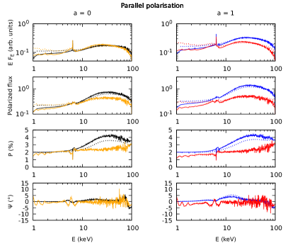
Figure 4.15: The total type-1 AGN emission in the $\theta=20\mbox{${}^{\circ}$}$ direction in the case of unpolarized primary radiation (solid lines) and the incident disc-corona emission in the polar direction (dotted lines). We display from top to bottom the energy-dependent flux (in arbitrary units, corrected for the primary power-law slope) and the corresponding polarized flux, polarisation degree and polarisation angle. From left to right: the case of unpolarized primary for $a=0$ and $a=1$ and the case of $2\%$ parallelly polarized primary for $a=0$ and $a=1$. The computations from Marin et al. (2018a) are displayed in black and blue. The new computations for ionized disc are displayed in yellow and red. The winds are neutral with the column density $N_{\textrm{H}}^{\textrm{wind}}=10^{21}\,\textrm{cm}^{-2}$. The column density of the torus is $N_{\textrm{H}}^{\textrm{eq}}=10^{24}\,\textrm{cm}^{-2}$. See Marin et al. (2018a) for the remaining parameters. Image adapted from Podgorný et al. (2024).

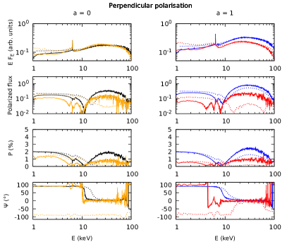
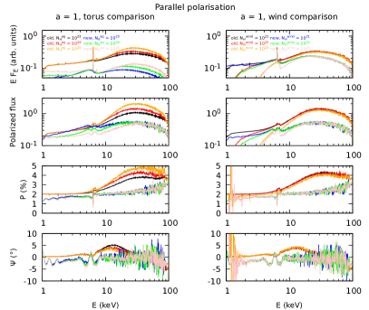
Figure 4.16: From top to bottom the energy-dependent flux (in arbitrary units, corrected for the primary power-law slope) and the corresponding polarized flux, polarisation degree and polarisation angle. Left: the same as in Figure 4.15, but for $2\%$ perpendicularly polarized coronal radiation for $a=0$ and $a=1$. Right: comparison of torus densities and polar wind densities for type-1 AGNs. The total AGN emission for the comparisons are in the $\theta=20\mbox{${}^{\circ}$}$ direction and for the case of $2\%$ parallelly polarized primary radiation and $a=1$. For the comparisons of different tori ($3^{\textrm{rd}}$ column from the left) we display the results for torus column densities: $N_{\textrm{H}}^{\textrm{eq}}=10^{23}\,\textrm{cm}^{-2}$ (black), $N_{\textrm{H}}^{\textrm{eq}}=10^{24}\,\textrm{cm}^{-2}$ (red), $N_{\textrm{H}}^{\textrm{eq}}=10^{25}\,\textrm{cm}^{-2}$ (orange) for the computations from Marin et al. (2018a) and the same torus column densities $N_{\textrm{H}}^{\textrm{eq}}=10^{23}\,\textrm{cm}^{-2}$ (blue), $N_{\textrm{H}}^{\textrm{eq}}=10^{24}\,\textrm{cm}^{-2}$ (green), $N_{\textrm{H}}^{\textrm{eq}}=10^{25}\,\textrm{cm}^{-2}$ (pink) for the new computations for ionized disc. The winds are neutral with the column density $N_{\textrm{H}}^{\textrm{wind}}=10^{21}\,\textrm{cm}^{-2}$. For the comparisons of different winds ($4^{\textrm{th}}$ column from the left) we display the results for wind column densities: $N_{\textrm{H}}^{\textrm{wind}}=10^{21}\,\textrm{cm}^{-2}$ (black), $N_{\textrm{H}}^{\textrm{wind}}=10^{22}\,\textrm{cm}^{-2}$ (red), $N_{\textrm{H}}^{\textrm{wind}}=10^{23}\,\textrm{cm}^{-2}$ (orange) for the computations from Marin et al. (2018a) and the same wind column densities $N_{\textrm{H}}^{\textrm{wind}}=10^{21}\,\textrm{cm}^{-2}$ (blue), $N_{\textrm{H}}^{\textrm{wind}}=10^{22}\,\textrm{cm}^{-2}$ (green), $N_{\textrm{H}}^{\textrm{wind}}=10^{23}\,\textrm{cm}^{-2}$ (pink) for the new computations for ionized disc. See Marin et al. (2018a) for the remaining parameters. The torus has the column density of $N_{\textrm{H}}^{\textrm{eq}}=10^{24}\,\textrm{cm}^{-2}$. Image adapted from Podgorný et al. (2024).

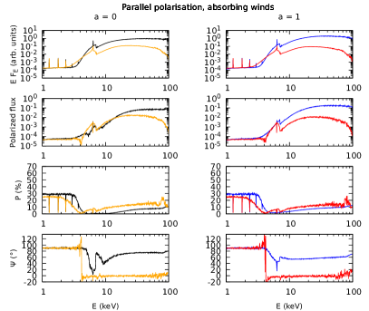
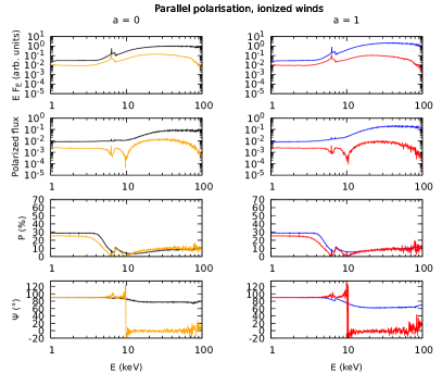
Figure 4.17: The total type-2 AGN emission in the $\theta=70\mbox{${}^{\circ}$}$ direction in the case of $2\%$ parallelly polarized coronal radiation. We display from top to bottom the energy-dependent flux (in arbitrary units, corrected for the primary power-law slope) and the corresponding polarized flux, polarisation degree and polarisation angle. From left to right: the case of absorbing winds with $N_{\textrm{H}}^{\textrm{wind}}=10^{21}\,\textrm{cm}^{-2}$ for $a=0$ and $a=1$ and the case of ionized winds for $a=0$ and $a=1$. The computations from Marin et al. (2018b) are displayed in black and blue. The new computations for ionized disc are displayed in yellow and red. The torus column density is set to $N_{\textrm{H}}^{\textrm{eq}}=10^{24}\,\textrm{cm}^{-2}$. See Marin et al. (2018b) for the remaining parameters. Image adapted from Podgorný et al. (2024).

The results can already serve for first-order estimates of X-ray polarisation of radio-quiet AGNs. All in all, we discovered more discrepancy between the old and new simulations for type-2 AGNs. This might sound surprising, because the spectropolarimetric properties of the central source should play a role mostly for unobscured sources. We discovered, however, some errors in the computations of type-2 AGNs in Marin et al. (2018b), where the total output of the simulation was, in an unknown way, wrongly rotated to resemble the central emission. This caused the type-2 AGNs to preserve a strong dependency on the central emission properties in Marin et al. (2018b), which we no longer see in the latest results. Our latest results for type-1 AGNs rather agree, but in the 10–100 keV band we obtained about half of the polarisation fraction that was previously estimated in Marin et al. (2018a). Regarding energy dependence for both type-1 and type-2 AGNs, we obtained most dissimilarities from the older publications rather in the hard X-rays (10–100 keV) than in the 2–8 keV band important for IXPE.

Let us first discuss in more depth the studied type-1 AGNs. We showed in Section 4.1 that even for the type-1 observers the composition and geometry of the equatorial scattering region greatly affects the X-ray polarisation properties of the reprocessed radiation. With the total emission results presented in this section we, however, estimate that the properties of the parsec-scale components may alter the X-ray polarisation degree output only up to a few % for type-1 AGNs with respect to the polarisation fraction of the bare nuclear component. Typically the parallelly polarized primary cases result in unaltered polarisation degree. The unpolarized primary cases result in $\approx 1\%$ additional polarisation with either parallel or perpendicular orientation (for meridional symmetry reasons), depending on the properties of the parsec-scale reprocessing components and observer’s inclination (see Section 4.1 for details). The perpendicularly polarized incident emission tends to be gradually depolarized on the output with energy: at soft X-rays preserving its original polarisation state and then reaching the unpolarized state at around 10 keV, continuing at even higher energies in parallel polarisation direction with increasing polarisation degree with energy. Similarly to the arguments for equatorial reprocessings that we used in Section 4.1, we see a competition between a dominantly perpendicularly polarized primary emission and dominantly parallelly polarized reprocessed radiation in the last case mentioned. As we showed in Section 3.1.1 with the KYNSTOKES code in lamp-post regime, especially for the neutral disc with low black-hole spin values, the reflection component is negligible compared to the primary in the soft X-rays. Hence, the primary radiation properties are rather preserved, at least towards the poles. In the equatorial directions, the nuclear emission may be parallelly polarized at all studied energies (see Figure A.35). The reprocessing in distant components then adds a parallelly polarized contribution to the total signal especially in the hard X-rays, where the photons are less absorbed. The energy transition for the cases with perpendicularly polarized corona appears sharper and at slightly lower energies than in Marin et al. (2018a) due to the model differences and due to choice of a particular inclination bin (see below).

In Marin et al. (2018a), a comparison for different torus and wind densities was provided for type-1 AGNs, which we also compare to our latest results in Figure 4.16 (right). Performing the same analysis, we reached a reasonable agreement for comparison of different wind densities, but we note again some differences of unknown origin for the torus comparisons. Part of the dissimilarities can be attributed to the choice of a particular inclination bin (see below). In general, we also observe a slight swing in the polarisation angle around the iron line at 6.4 keV with respect to the nearly energy-independent polarisation angle seen in Marin et al. (2018a). This may be due to the lower predicted polarisation in the line itself (after the reprocessing, which generally adds polarisation to an unpolarized fluorescent emission at the photon creation location), as the polarisation angle is undefined for unpolarized light.

As in Marin et al. (2018b), for type-2 AGNs we obtain the same prediction for $\gtrapprox 25\%$ perpendicularly polarized emission in the soft X-rays that arises from high absorption in the dusty torus and high contribution to polarisation from the polar winds, which reflect dominantly in the right scattering angles in the meridional plane. The trade-off for detectability by polarimeters at these energies is obviously the low X-ray flux caused by Compton thickness. As advertised before, we conclude that the GR effects do not play any role for the type-2 X-ray polarimetric observers. More generally speaking, the spectropolarimetric properties of the primary radiation and the inner-accreting region characteristics, now also probed for partial ionization of the disc atmospheres thanks to the latest KYNSTOKES code, are expected to be to a large extent washed out for Compton-thick AGNs. In the hard X-rays, the resulting emission is parallelly polarized with a slight increase with energy up to $\approx 10\%$ near 100 keV.

We discovered that in general the results are highly dependent on the inclination bin chosen when proceeding with 20 inclination bins linearly spaced in cosine of $\theta$, as we did. We opted for $\cos{\theta}=0.375$ and $\cos{\theta}=0.975$ in the simulations for type-2 and type-1 AGNs, respectively, being close to the stated $\theta=70\mbox{${}^{\circ}$}$ and $\theta=20\mbox{${}^{\circ}$}$ viewing angles stated in Marin et al. (2018a, b). But if, for example, the neighboring simulation bins $\mu_{\textrm{e}}=0.325$ and $\mu_{\textrm{e}}=0.925$ are selected, $\Psi$ may change in the order of a few degrees and $p$ in the order of $1\%$. The energy transition in $p$ and $\Psi$ that served as a diagnostic tool in Marin et al. (2018a, b) is shifted more by the inclination bin chosen than by any claimed effects therein. Results from Section 4.1 indicate the the choice of the half-opening angle (fixed to $H^{\prime}=60^{\circ}$ here) will also affect the X-ray polarisation properties at least for the type-2 AGNs. The $\theta$ and $H^{\prime}$ parameters, alongside composition, shape and possible misalignment of the parsec-scale components thus appear to be determinative for the result, especially for the type-2 AGNs, and should be estimated before any more detailed interpretation from the X-ray polarimetric data is drawn. Constraints on such parameters can be obtained by additional modeling and from X-ray spectroscopic observations or polarimetry in other wavelengths for a particular AGN (e.g. Antonucci and Miller, 1985; Smith et al., 2004; Goosmann and Matt, 2011; Gaskell et al., 2012; Marin et al., 2018c; Hutsemékers et al., 2019; Marin et al., 2020; Stalevski et al., 2023).

We envision that the simulation results presented here would be also more diverse, if non-isotropic coronal emission was implemented to KYNSTOKES, but the true sensitivity to this assumption cannot be tested in the present scope. We also note that we used the semi-isotropic illumination of the parsec-scale components in the subsequent MC simulation, which is another simplification that could be tested for model sensitivity perhaps more easily, just by binning in higher angular resolution in the STOKES input and by relaunching the simulations. It would require, however, some additional technical effort due to the STOKES v2.07 code’s architecture. Any more sophisticated inner-accreting model is also possible to test within STOKES (more easily if assumed to be of negligible size, as in the results above), if the expected central source emission is provided in a tabular format. We expect here an effect on the studied cases of type-1 AGNs, because even with a handful of first IXPE results, coronal properties of some AGNs were indeed already constrained through these observations (Marinucci et al., 2022; Gianolli et al., 2023; Tagliacozzo et al., 2023; Ingram et al., 2023b, see Chapter 5 for detailed discussion).

Chapter 5 X-ray polarimetric observations of accreting black holes

In this chapter, we provide the observational analysis and perspective with the latest operating or planned X-ray polarimeters. Since X-ray polarimetry is currently experiencing a boom thanks to the IXPE, the results presented in this chapter and their context are highly dynamic and may be in some cases outdated shortly after the submission of the manuscript.

During the first year and a half of operations, IXPE observed a number of accreting black holes, complementarily to the observations of other interesting X-ray sources that were outlined in Section 1.2.3. A specific category contains blazars, which show very distinct properties due to their orientation towards us (Di Gesu et al., 2022; Ehlert et al., 2022; Liodakis et al., 2022; Di Gesu et al., 2023; Ehlert et al., 2023; Kim et al., 2024; Marshall et al., 2023; Middei et al., 2023; Peirson et al., 2023). In terms of observational traits, inclined accreting black holes exhibit properties rather closer to the previously mentioned weakly magnetized accreting neutron stars, which in addition to the disc, corona and more distant components possess a boundary layer of the compact object.

Radio-quiet accreting black holes that we primarily study in this dissertation are expected to be X-ray polarized mostly due to scattering and absorption mechanisms, because ordered magnetic fields are not strongly present. The first IXPE results confirm the long-standing theoretical expectations (e.g. Soffitta, 2017; Weisskopf et al., 2022) that sources possessing strong and ordered magnetic fields will be generally higher X-ray polarized than those that do not. Thus, it was rather a pleasant surprise that many accreting black holes still revealed a few percent polarized X-rays in 2–8 keV. We will now introduce these IXPE results in more detail.

According to the expectations, the observed bright Galactic XRBs provided so far more positive polarisation detections with IXPE than the generally fainter extragalactic AGNs. However, we have argued enough with all the numerical models presented that even an observed polarisation upper limit can still be theoretically highly informative.

We will thus begin with presenting the recent X-ray polarimetric discoveries in accreting stellar-mass black holes and then continue with the more mysterious (and arguably more complex) AGN analogs. As part of this dissertation, we contributed to the discussions in the IXPE science analysis and simulations working group – in the topical working groups of accreting stellar-mass black holes and radio-quiet AGNs. We participated in the observation analyses of the IXPE team campaigns listed below and loosely affected the large collaboration efforts by the ongoing theoretical work presented in this dissertation. If more detailed investigations were performed for a particular source as part of this dissertation, we devote to it a specific section below. Simultaneously, we carried simulations that should assist with future observational planning for accreting black holes with IXPE or other X-ray polarimeters mentioned in Section 1.2.2. These are also provided below.

5.1 Accreting stellar-mass black holes

The first observed XRB by IXPE was Cygnus X-1 (Krawczynski et al., 2022), caught in its hard spectral state in May 2022 ($4.01\%\pm 0.20\%$ in 2–8 keV at a $68\%$ confidence level) and June 2022 ($3.84\%\pm 0.31\%$ in 2–8 keV at a $68\%$ confidence level). The obtained polarisation is perfectly aligned with the observed projected direction of the radio jet in the source (Miller-Jones et al., 2021) in both observations. Most importantly, this confirms that a) the regions many orders of magnitude smaller in physical size that IXPE covered are inherently linked to the large scale jet emission and b) that the corona is more likely equatorially elongated (but note the results of Dexter and Begelman, 2024; Moscibrodzka, 2023, which are in contradiction to that). Number of explanations occurred for the surprisingly high polarisation degree, the most promising being higher inclination of the accretion disc or coronal medium than the orbital inclination ($\theta=27.5^{\circ}\pm 0.8^{\circ}$, Miller-Jones et al., 2021) (Krawczynski et al., 2022; Zdziarski et al., 2023), or an outflowing Comptonization component at relativistic speeds (Poutanen et al., 2023; Dexter and Begelman, 2024). In May 2023, Cygnus X-1 was observed again by IXPE, but in its soft state ($1.99\%\pm 0.17\%$ in 2–8 keV at a $68\%$ confidence level, Dovčiak et al., 2023c; Jana and Chang, 2024, Steiner et al., in prep.). Although the polarisation degree decreased, the polarisation angle remained very similar, parallel with the jet, despite strong presence of the thermal component in 2–8 keV. This raises questions on the origin of polarisation in the soft state, as usually the thermal disc emission models predict emergent polarisation parallelly to the accretion disc (see Section 1.5.1). But it could still be the case that the polarisation of thermal component was just diluting the still dominant polarisation from Comptonization component, orthogonally oriented.

Another example of a hard-state XRB with observed high X-ray polarisation by IXPE was Swift J1727.8-1613 (Dovčiak et al., 2023b, a; Veledina et al., 2023a; Ingram et al., 2023a), a Galactic black-hole candidate discovered in August 2023 through a strong X-ray outburst (Kennea and Swift Team, 2023; Negoro et al., 2023). Although not much information about the object is known yet, it was caught first in the hard state and subsequently in transition to the soft state. The IXPE detection of $4.71\%\pm 0.27\%$ 2–8 keV polarisation (at a $68\%$ confidence level) in the hard state, aligned with the observed submillimeter polarisation (which is about twice lower, Vrtilek et al., 2023), promises similar polarisation emergence conditions to the hard state of Cygnus X-1. During the transition to the soft state, the polarisation properties seem again not to be changed significantly (Ingram et al., 2023a), similarly to the Cygnus X-1 data [Steiner et al., in prep.], which is much surprising, as the spectral energy distribution changes significantly. QPOs were already detected in the IXPE flux data of Swift J1727.8-1613 (Ingram et al., 2023a; Veledina et al., 2023a), so additional detailed analysis may reveal the expected corresponding swing in X-ray polarisation angle. Thus altogether, this newly discovered source promises gold mines for our understanding of accreting black holes, not only through the eyes of X-ray polarimetry, as many multiwavelength campaigns are ongoing.

IXPE observed a number of XRB sources in the soft spectral state, which may be classified as more typical high/soft states (cf. Section 1.4) than the state-transited two sources mentioned above. The first one being 4U1630-47 ($8.3\%\pm 0.3\%$ in 2–8 keV at a $68\%$ confidence level), observed in September 2022 and providing surprisingly high polarisation degree, increasing with energy (Rawat et al., 2023; Kushwaha et al., 2023a; Ratheesh et al., 2024). The polarisation angle was nearly constant with energy, however, the orientation of the source on the sky from other data is unknown. We will return to the intricate possibilities of interpretation of such polarisation state in the soft state below, but what is perhaps equally puzzling is little change in polarisation when transitioning into a different state, similarly to the cases of Cygnus X-1 and Swift J1727.8-1613. The source was observed again in March of 2023 in the steep power-law state (Rodriguez Cavero et al., 2023) and although the polarisation has decreased ($6.8\%\pm 0.2\%$ in 2–8 keV at a $68\%$ confidence level), the polarisation angle remained almost unchanged. Albeit neither here, nor in the cases of Cygnus X-1 and Swift J1727.8-1613, the second set of observations does not represent an XRB in a “clear” spectral state, we note that the state transitions occurred in two different directions (departing from the high/soft state in 4U1630-47 and departing from the low/hard state in Cygnus X-1 and Swift J1727.8-1613). If the thermal radiation was polarized perpendicularly to the disc, it would mean significant theoretical reconsiderations.

So far, no XRB was caught by IXPE in a clear high/soft state that would have both, statistically significant polarisation detection and known orientation on the sky. IXPE observed the prototypical soft-state XRB, LMC X-1, in October 2022 (Podgorný et al., 2023d). It meant only a hint of $1.0\%\pm 0.4\%$ polarisation (in 2–8 keV at a $68\%$ confidence level, but more securely stating that the observed polarisation is below the $M\!D\!P_{99\%}=1.1\%$ in 2–8 keV, hence statistically insignificant at a $99\%$ confidence level) in the projected ionization cone direction observed in optical band (Cooke et al., 2008), i.e. most likely perpendicularly to the projected accretion disc plane. Low orbital inclination, if linked to the inner X-ray source inclination, is in line with the low observed polarisation. We also note that we observed a slight dilution of the thermal radiation by hard X-ray power-law, which may be another reason for low polarisation due to mixture of two perpendicularly polarized components. Thus, the LMC X-1 observation does not exclude the Chandrasekhar-Sobolev predictions for thermally radiating discs, if the power-law component was polarized perpendicularly to the thermal one and was driving the resulting polarisation (i.e. if it was diluted by the thermal emission in polarisation, not vice versa). As this source is remarkably stable, additional IXPE observations of LMC X-1 may, however, reveal the true orientation of polarisation of thermal radiation as well as prove a variability with orbital phase, which was detected with low significance during the first IXPE observation (Podgorný et al., 2023d). The latest X-ray spectroscopic analysis suggests a presence of a warm and optically thick surface skin of the disc (Zdziarski et al., 2024), which is in accordance with the inverse disc temperature-luminosity relation for LMC X-1 (Gierliński and Done, 2004) and which could affect the resulting polarisation. Due to low statistics, it was not possible to constrain the black-hole spin, nor disc inclination from X-ray polarimetry in this source, using the KYNBBRR code. Especially the determination of spin in (not only) LMC X-1 is of paramount importance for gravitational-wave, stellar-evolution and cosmological studies (e.g. Qin et al., 2019; Belczynski et al., 2021; Mehta et al., 2021; Fishbach and Kalogera, 2022; Shao and Li, 2022).

The last two XRBs caught in true soft state were 4U1957+115 ($1.88\%\pm 0.37\%$ in 2–8 keV at a $68\%$ confidence level) and LMC X-3 ($3.2\%\pm 0.6\%$ in 2–8 keV at a $68\%$ confidence level), observed in May 2023 and July 2023, respectively (Garg et al., 2023; Majumder et al., 2023; Svoboda et al., 2024; Kushwaha et al., 2023b; Marra et al., 2023). They both show increasing polarisation with energy and constant polarisation angle with unknown relation to the system projected orientation. 4U1957+115 is possible to fit with conventional models of relativistic thermally radiating standard discs, confirming a rather highly spinning black hole (Marra et al., 2023). However, the case of LMC X-3 is already slightly better fitted with thick disc atmospheres alongside lower spin values (Svoboda et al., 2024), similarly to the 4U1630-47 case, where even relativistic outflowing velocities are needed to explain the high polarisation degree to emerge in such scenarios (Ratheesh et al., 2024). Thus, it suggests itself that the low spin of 4U1957+115 fitted with conventional models may not be of high confidence, if the same polarisation models will fail at other sources with similar spectral properties.

Last but not least, two XRBs were observed in highly obscured conditions. The ULX object SS433 was observed in its eastern lobe ($17.3\%\pm 4.3\%$ in 2–5 keV at a $68\%$ confidence level, Kaaret et al., 2024). The extremely high polarisation may be attributed to the magnetic fields accompanying the jet, being oriented parallel to the observed projected jet direction (Stirling et al., 2004) and producing synchrotron emission polarized in the perpendicular direction (Kaaret et al., 2024). Some reflection of the X-rays from inner side of the obscuring funnel may play a role too, because the polarisation is in the direction perpendicular to the projected jets. The latter polarisation generation mechanism is certainly applicable to the case of Cygnus X-3, which shows only a reflected X-ray power-law in spectra and was caught in the hard and intermediate (minor flaring) states in October and November 2022 ($20.6\%\pm 0.3\%$ in 2–8 keV at a $68\%$ confidence level) and December 2022 ($10.4\%\pm 0.3\%$ in 2–8 keV at a $68\%$ confidence level), respectively (Veledina et al., 2023b). The polarisation angle is orthogonal to the observed direction of polar ejecta (Fender et al., 1999) within the measurement uncertainties. We will elaborate more below on this source, as models developed in this dissertation were used for the data interpretation. As described in Section 4.1, it is no surprise that highly obscured accreting black holes may also provide large polarisation by means of scattering and absorption only, because the isotropy of emission inside the system is significantly reduced.

5.1.1 Analysis of the Cygnus X-1 IXPE observations

Only a small fraction of IXPE observations of compact accreting objects showed significant disc reflection, where the KYNSTOKES model developed in this dissertation would be directly applicable. Apart from the weakly magnetized neutron star Cygnus X-2 (Farinelli et al., 2023), where the analysis with KYNSTOKES is ongoing, we used it for the first IXPE observation of Cygnus X-1 (Krawczynski et al., 2022). In particular we were curious if the results in the lamp-post regime could explain the observations. Mostly the observed polarisation angle disfavored the lamp-post coronal types, as the estimates from KerrC, COMPPS and MONK codes (that are focused on the Comptonization component) suggested, although a possibility for the observed polarisation produced by relativistically outflowing lamp-post corona was recently reexamined by Dexter and Begelman (2024); Moscibrodzka (2023). In any such lamp-post assumptions, a first-order estimate on the reflection fraction versus polarisation degree gained by reflection can be made with the KYNSTOKES model in lamp-post regime, which was described in Section 3.1 and which provides almost exclusively polarisation orientation parallel with the rotation axis and polarisation degree increasing with energy, supporting the observed trends in Cygnus X-1 (Krawczynski et al., 2022). The polarisation by reflection is treated through Chandrasekhar’s diffuse formulae in KerrC and is neglected in MONK. Therefore we still tested possibilities that KYNSTOKES offers, especially regarding the truncated accretion disc and extreme incident polarisation, because if the $\approx 10\%$ of reflection fraction in 2–8 keV (Krawczynski et al., 2022) could be in any scenario $40\%$ polarized, it could explain the $4\%$ total polarisation fully for an unpolarized corona. Figures similar to Figure 3.11 were drawn for a large parametric space. It was concluded that with the observed 2–8 keV disc reflection fraction of $\approx 10\%$, for any disc truncation the polarisation gained by reflection in the equatorial plane cannot be significant enough for lamp-posts to lead the observed total polarisation values.

Another numerical experiment, in collaboration with Wenda Zhang and Michal Dovčiak and later on also with Sudeb Ranjan Datta, was made to trace the disc illumination with MONK and to obtain the radius and energy-dependent spectropolarimetric values in the equatorial plane with MONK. All available parameter constraints on Cygnus X-1 in the literature were considered. The inner disc inclination was assumed as the orbital one (Miller-Jones et al., 2021). The black-hole spin was assumed as $a=0.998$. For simplicity we also assumed the inner disc radius to extend to the ISCO in this experiment. The lamp-post corona in MONK was static, spherical, had a radius of $10\,r_{\textrm{g}}$ and Thomson optical depth $\tau_{\textrm{T}}=0.6$ and was located at height $12\,r_{\textrm{g}}$. Then we used KYNSTOKES in the lamp-post regime with the same polarisation state and primary power-law ($\Gamma=2$) prescribed at the corona and studied the reflected-only output. This was done at each energy band and per each disc ring, subsequently superposed.

Although the superposed KYNSTOKES results were similar to the already presented results with initial conditions independent of energy and disc radius (see Section 3.1), we concluded that a more realistic estimate for direct interpretation of X-ray polarisation of XRBs in the hard state would be possible only after either a) implementing non-isotropic coronal emission into KYNSTOKES or b) linking only the disc reprocessing and relativistic radiative transfer from the disc to the distant observer from KYNSTOKES directly to the MONK equatorial output, as a subroutine of MONK, which currently neglects coronal photons reflected from the disc. The option b) is currently being investigated, being limited by required MC photon counts needed for obtaining the polarisation input in the equatorial plane in sufficient resolution within reasonable computational times. In the above mentioned attempt with KYNSTOKES, when combining the obtained reflected-only signal with the direct primary from MONK and with the thermal radiation from KYNBBRR, all unabsorbed and normalized relative to each other according to the spectral analysis of Cygnus X-1 (Krawczynski et al., 2022), we could not obtain polarisation higher than $\approx 1\%$ on average in the IXPE band, although an increase with energy was obtained. The polarisation angle in 2–8 keV was also misaligned by $\approx 30^{\circ}$ with the principal axis. The resulting total simulation and component decomposition is shown in Figure 5.1.

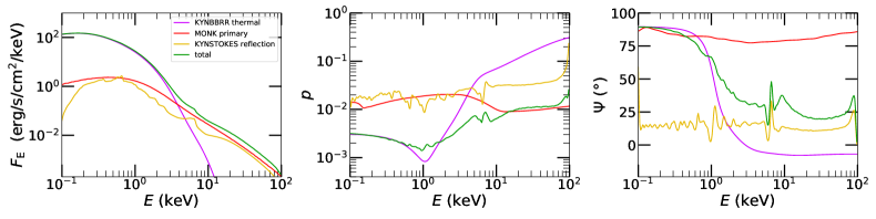
Figure 5.1: Combined unfolded and unabsorbed simulation of the main spectral components observed in the hard state of Cygnus X-1 in the IXPE related observational campaign in May of 2022 (Krawczynski et al., 2022). The thermal component was simulated by KYNBBRR model, the lamp-post primary emission component was simulated by MONK code and the relativistic disc reflection component was simulated by KYNSTOKES. We display the spectrum (left) and the corrsponding polarisation degree (middle) and angle (right).

5.1.2 Analysis of the 4U1630-47 and LMC X-3 IXPE
observations

The IXPE observations of XRBs 4U1630-47 and LMC X-3 in their soft states, which were difficult to explain using standard models, were a motivation for more theoretical work during this dissertation. The model for thermal radiation passing through a passive comoving atmosphere that was developed based on the TITAN, CLOUDY and STOKES codes, was fully described in Section 2.2. Here we will add information on how this model was used for direct comparison with the data in Ratheesh et al. (2024) and Svoboda et al. (2024). Although such model is in many senses non-standard, it is currently the only modeling direction, alongside the bremsstrahlung models of Krawczynski et al. (2023), which allows for high enough polarisation degree of X-ray disc emission with polarisation increase with energy in 2–8 keV. The produced polarisation angle is constant with energy, which is as well in line with the data. However, if any clear evidence for 2–8 keV polarisation of thermal disc emission from XRBs came in the future alongside known projected primary disc axis orientation of the source, which would be parallel to the detected polarisation, then the presented model would not be applicable to explain such data, because it produces polarisation direction parallel with the disc. The same validity limit holds for the assumption of high ionization, which we use according to the X-ray spectral characteristics of 4U1630-47 and LMC X-3, based on simultaneous spectral observational campaigns to the IXPE exposures (Ratheesh et al., 2024; Svoboda et al., 2024).

Because the first IXPE observation of 4U1630-47 in the soft state meant a particularly demanding data interpretation due to the measured extreme mean polarisation degree, we first made some preliminary estimates with the local absorbing atmosphere model in high ionization limit (see Section 2.2.2), whether it can roughly explain such polarisation without any disc integration and relativistic effects. Figure 1.22 showed already the most probable 2–8 keV polarisation degree value and the most probable polarisation degree value in the lowest energy bin from Ratheesh et al. (2024), plotted over the inclination dependence of classical analytical X-ray polarisation estimates. As we argued in Section 2.2.2, the polarisation value at 2 keV should already be close to the pure-scattering energy-independent plateau expected at soft X-rays, which is supported by both our model and the model of Valery Suleimanov (Ratheesh et al., 2024), and which could be also altered by Faraday rotation towards lower energies (Davis et al., 2009). Hence, at 2 keV the result can be roughly approximated by the Chandrasekhar-Sobolev profile for semi-infinite atmosphere with scattering-only induced polarisation properties. For the 2–8 keV average polarisation degree value, we have to add the absorption effects that increase polarisation in such scenarios, which can be done through the Loskutov-Sobolev model (Loskutov and Sobolev, 1981). Both analytical approximations match with the data near 2 keV and at 2–8 keV roughly at local inclinations $\delta_{\textrm{e}}\approx 80^{\circ}$ (see Figure 1.22), which forms a first-order theoretical lower limit on inclination, as the relativistic disc integration will require even higher values.

Using the XSPEC table model generator described in Appendix D, we created a tabular FITS spectropolarimetric model suitable for XSPEC that contained the smoothed polynomial approximation of polarisation degree with energy in 1–20 keV, which was described in Section 2.2.2. Fitting this absorbing atmosphere model directly to the 4U1630-47 data without any relativistic integration delivers another simple estimate on the required inclination, alongside the model parameter $\tau_{\textrm{T,max}}$. Figure 5.2 shows the resulting fit of polarisation degree with energy in XSPEC. Despite the dependency on $T_{\textrm{BB}}$ value, we conclude that, for the mean $kT_{\textrm{BB}}=1.15$ keV obtained from simultaneous campaigns that were described in Ratheesh et al. (2024), the results match well with $\tau_{\textrm{T,max}}\approx 5$ and $\theta\approx 84^{\circ}$. This is already extreme compared to the usual $\theta\approx 78^{\circ}$ eclipsing upper limits on inclination obtained for XRBs in e.g. de Jong et al. (1996).

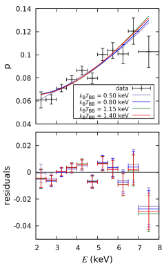
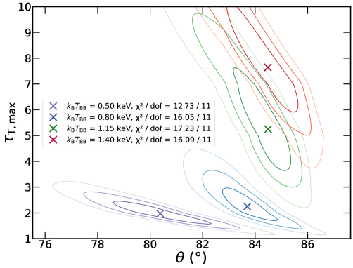
Figure 5.2: Best-fit local atmosphere solutions of polarisation degree, $p$, versus energy (left) and 2D contours at $1\sigma$, $2\sigma$, $3\sigma$ levels around their value in the {$\theta$,$\tau_{\textrm{T,max}}$} space (right) obtained with XSPEC by fitting the energy-dependent polarisation degree data with smoothed TITAN and STOKES models, fully described in Section 2.2.2, for $kT_{\textrm{BB}}=0.50$, $0.80$, $1.15$ and $1.40$ keV. The $\chi^{2}/\textrm{dof}$ values are indicated. The underlying data are from the first IXPE observation of the XRB 4U1630-47 in the soft spectral state (Ratheesh et al., 2024). Image adapted from Ratheesh et al. (2024).

As described in Section 2.2.2 and Chapter 3, the smoothed local model was then implemented to the KYNBBRR code, forming a new variant KYNEBBRR. The implementation and fitting with KYNEBBRR were performed by Michal Dovčiak and Jiří Svoboda and were not part of this dissertation. A proper relativistic integration using this model for the first IXPE 4U1630-47 dataset required a relativistically outflowing atmosphere (with $v\approx 0.5c$), alongside high optical thickness ($\tau_{\textrm{T,max}}\approx 7$) and high inclination ($70^{\circ}\lessapprox\theta\lessapprox 75^{\circ}$) (Ratheesh et al., 2024). The aberration-induced polarisation was not necessary for the data fit of the IXPE LMC X-3 observation with KYNEBBRR, but the optically thick absorbing and Compton-scattering atmosphere provided also here a lower reduced $\chi^{2}$ than using the relativistic thermal emission model variant KYNBBRR with pure-scattering Chandrasekhar’s prescription for locally emergent polarisation, but still assuming the Novikov-Thorne accretion disc (Svoboda et al., 2024). For the case of LMC X-3, a slim disc instead of standard geometrically thin accretion disc would perhaps suit better also in polarisation, as it does already in pure spectral analysis (Svoboda et al., 2024). Nonetheless, the standard accretion disc theory is significantly challenged through such discoveries by IXPE.

5.1.3 General observational prospects for equatorially obscured sources and analysis of the Cygnus X-3 IXPE observations

We will be more detailed in description of the analysis in Cygnus X-3 than with the other sources, because additional modeling was performed as part of this dissertation to support the interpretations of the IXPE discoveries published in Veledina et al. (2023b). The two aforementioned observations of Cygnus X-3 by IXPE were separated by about 2 months. Similarly to the discovery paper of Veledina et al. (2023b), let us call the first observation “main” and the second target-of-opportunity observation “ToO”. We will work only with the time-averaged values, although a small variability of polarisation with orbital phase was detected. The study of Veledina et al. (2023b) contains a leading analytical model of single-scattering reflection on conical equatorial outflows, which is compared with the energy-independent 3.5–6 keV part of the X-ray polarisation data. The observations are interpreted as reflection from the inner walls of such funnel, which is assigned a ULX-like narrow opening angle. Apart from our theoretical investigations of reprocessings in distant equatorial obscurers that were already described in Section 4.1, we performed 2–8 keV simulations that include direct radiation and remove neutral hydrogen from the otherwise same list of absorbers, as in Section 4.1, to be closer to the assumed hydrogen-poor environment of outflows in Cygnus X-3 (Fender et al., 1999; Kallman et al., 2019). The results were analyzed and plotted in Veledina et al. (2023b) in the same way and in direct relation to the analytical models studied therein. Soon after, we decided to elaborate in more depth on the MC analysis and we provided a full range of examples and an extended discussion as part of Podgorný et al. (2023c). The extended discussion, including visual presentation of the full atlas of results (exceeding those that fitted in Podgorný et al., 2023c), is presented in this section and Appendix A.

The models described in Section 4.1 are particularly useful for observational analysis of Cygnus X-3, because unlike the analytical models, they allow to assess the role of partial transparency and partial ionization, although the latter only simplistically by means of adjusting free electron density (thus introducing more polarisation at soft X-rays with respect to a proper treatment of ionization). The partial transparency has been in fact proposed in Veledina et al. (2023b) to play a role in decrease of the observed polarisation degree from the main observation to the ToO observation. Apart from changing the chemical composition and adding direct radiation in this section, we also fix the mid torus distance to $R^{\prime}=0.5$ (again the true units are unimportant for polarisation production in our model design) and unfreeze $r_{\textrm{in}}^{\textrm{torus}}$. In this way, such additional models are an opportunity to test the sensitivity of results to previously adopted assumptions. Otherwise the model setup is unchanged from Section 4.1. We do not add any polar scatters, we do not introduce misalignment, nor clumpiness or non-uniform densities. We keep the convention of a positive and negative polarisation degree, corresponding to the parallel and perpendicular polarisation angle with respect to the axis of symmetry, respectively, because again no relativistic effects are assumed and the result cannot be any other than orthogonal or parallel with respect to the leading directions.

In fact, the orientation of Cygnus X-3 on the sky is known not only thanks to observed radio-loud ejecta (Fender et al., 1999), but also to the corresponding IR and submillimeter polarisation (Martí et al., 2000; Miller-Jones et al., 2004; Jones et al., 1994). The X-ray polarisation obtained with IXPE is perpendicular to the projected jet directions within the measurement uncertainty (Veledina et al., 2023b). This means that when comparing to the Cygnus X-3 data, we will focus on those parts of the parameter space where negative polarisation is expected and where type-2 viewing angles apply, as the spectra confirm a highly obscured source. However, we keep below the presentation of the full parameter space, as the presented models may be useful for interpretation of other IXPE observations in the future and they are distinct from the models described in Section 4.1 that served for more theoretical understanding of the reprocessing mechanisms. Similar obscuration conditions have been discussed in the context of IXPE analysis of the type-2 AGN Circinus Galaxy (Ursini et al., 2023b), the ULX object SS433 (Kaaret et al., 2024) and the accreting Be-transient X-ray pulsar LS V +44 17/RX J0440.9+4431 (Doroshenko et al., 2023). More observations of equatorially obscured accreting compact objects are likely to be performed by IXPE or other forthcoming X-ray polarimeters. Reprocessing in distant equatorial covering regions was also considered in the IXPE analysis of the (unobscured) AGN NGC 4151 (Gianolli et al., 2023).

Only the cases of $\Gamma=2$, $\Gamma=3$ and unpolarized and $4\%$ parallelly polarized emission (inspired by the observed value in the hard state of Cygnus X-1 Krawczynski et al., 2022) were computed. We considered 40 bins in inclination in the same linear spacing and range as with the 20 bins treated in Section 4.1. This is because we will plot the results in form of polarisation heatmaps in the $\{\theta,H^{\prime}\}$ space, to be able to directly compare the MC model to the analytical results provided in figure 4 of Veledina et al. (2023b), or to figure 6 of Ursini et al. (2023b) that used the Ghisellini et al. (1994) MC code for the interpretation of the type-2 AGN in Circinus Galaxy. The new simulations were performed with $N_{\textrm{tot}}=10^{10}$ simulated photons, which meant roughly 2 months to compute all on the available institutional clusters. As it will be shown below, even though the same energy binning as in Section 4.1 was adopted, the photon statistics are barely enough for energy-dependent analysis in 3 bins across 2–8 keV. Because neutral hydrogen was removed, we describe the results in terms of equatorial density $N_{\textrm{He}}^{\textrm{eq}}$ of the remaining most abundant element, which is neutral helium. We believe that such values are then more informative to an experienced reader than if we had recalculated to the usual $N_{\textrm{H}}^{\textrm{eq}}$. Both $N_{\textrm{He}}^{\textrm{eq}}$ and $\tau_{\textrm{e}}^{\textrm{eq}}$ values are scaled accordingly, to represent similar conditions to the two density cases and three partial ionization cases that were studied in Section 4.1.

We begin with analyzing the results in the integrated 2–8 keV band and only turn in later stages to the advantages of energy-dependent analysis. Figure 5.3 shows the heatmaps of polarisation degree in the $\{\theta,H^{\prime}\}$ space for selected cases in $N_{\textrm{He}}^{\textrm{eq}}$ and $\tau_{\textrm{e}}^{\textrm{eq}}$ that show the expected depolarisation by lowering density and/or ionization. When testing for particular examples of even lower densities and lower ionization levels (not shown), we obtained the limit of complete depolarisation. We obtained the general pattern of two distinct branches of solutions for type-2 observers, consistently with the analytical models in Veledina et al. (2023b) and MC simulations in Ursini et al. (2023b) (only the upper branch is observable in the range of figure 6 therein). The dashed black lines mark the grazing inclination angles. The main observation is marked in black rectangles, considered as $p=21\%\pm 3\%$ in 2–8 keV within simulation uncertainties. The ToO observation is marked in green rectangles, considered as $p=10\%\pm 3\%$ in 2–8 keV within simulation uncertainties. The white regions represent empty bins, where the results did not converge within reasonable computational times to provide MC results with reasonable numerical noise. The panels are shown for a general Case B obscurer with $b^{\prime}=R^{\prime}/4$, unpolarized primary and $\Gamma=2$. Figures A.37–A.42 provide examples of other geometries and primary radiation properties plotted in the exact same way. The lower branch of solutions is preferred for the interpretation of Cygnus X-3, as the steep increase in polarisation between the grazing angle line and the upper contour of observed values suggests high time variability of polarisation, which is not observed (Veledina et al., 2023b).

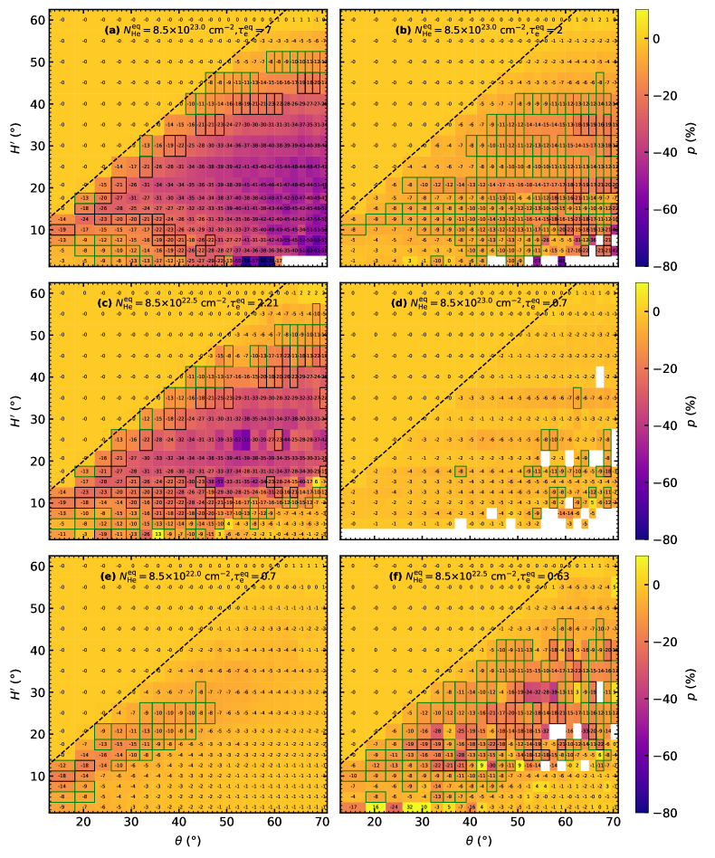
Figure 5.3: In the color code we show the STOKES model polarisation degree, $p$, integrated in 2–8 keV for the Case B elliptical equatorial obscurer with $b^{\prime}=R^{\prime}/4$ with respect to various inclinations $\theta$ and half-opening angles $H^{\prime}$. All photons are registered and the black dashed lines mark the grazing inclination angles. The black and green rectangles represent the simulation results roughly matching the main and ToO IXPE observations, respectively, of an X-ray binary system Cygnus X-3, extensively described in Veledina et al. (2023b). We show the case of unpolarized primary radiation with $\Gamma=2$. The left column shows the results for high ionizations, how they differ when lowering the column densities, i.e. from top to bottom we show (a) $N_{\textrm{He}}^{\textrm{eq}}=8.5\times 10^{23.0}\ \textrm{cm}^{-2}$ and $\tau_{\textrm{e}}^{\textrm{eq}}=7$, (c) $N_{\textrm{He}}^{\textrm{eq}}=8.5\times 10^{22.5}\ \textrm{cm}^{-2}$ and $\tau_{\textrm{e}}^{\textrm{eq}}=2.21$, (e) $N_{\textrm{He}}^{\textrm{eq}}=8.5\times 10^{22.0}\ \textrm{cm}^{-2}$ and $\tau_{\textrm{e}}^{\textrm{eq}}=0.7$. In top right and center right we show the highest density case for lower ionization levels, i.e. (b) $N_{\textrm{He}}^{\textrm{eq}}=8.5\times 10^{23.0}\ \textrm{cm}^{-2}$ and $\tau_{\textrm{e}}^{\textrm{eq}}=2$ and (d) $N_{\textrm{He}}^{\textrm{eq}}=8.5\times 10^{23.0}\ \textrm{cm}^{-2}$ and $\tau_{\textrm{e}}^{\textrm{eq}}=0.7$, respectively. The (f) bottom right panel shows the moderate density case for lower ionization, i.e. $N_{\textrm{He}}^{\textrm{eq}}=8.5\times 10^{22.5}\ \textrm{cm}^{-2}$ and $\tau_{\textrm{e}}^{\textrm{eq}}=0.63$. Image adapted from Podgorný et al. (2023c).

To be able to evaluate the impact of single-scattered photons, we repeated all simulations with registering only the photons that scattered once before reaching the detectors in the MC simulation. In Figure 5.4, we plot the corresponding results in the same way for the cases considered in Figure 5.3. In the single-scattering regime, we obtain even closer solutions to the analytical single-scattering model adopted as leading in the 3.5–6 keV band in Veledina et al. (2023b). Similar comparison conclusions apply for the single-scattering regimes in other geometries and for other primary radiation cases tested by us. There is still a principal difference between the analytical single-scattering model in Veledina et al. (2023b) from our “single-scattering regime”, because we still consider the absorption of photons. The leading model in Ursini et al. (2023b) (figure 6) examines a truly neutral absorber, thus providing perhaps more dissimilar results to ours in the full regime, although a detailed one-to-one comparison would be required for further commentary on possible modeling discrepancies of this model with respect to ours.

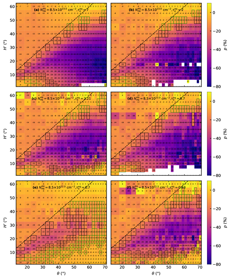
Figure 5.4: The same as in Figure 5.3, but for registered single-scattered photons only. Image adapted from Podgorný et al. (2023c).

Despite the modeling differences of the STOKES simulations presented here in the full regime, with respect to the results presented in Section 4.1, and despite the inclusion of spectral lines in the studied full 2–8 keV range, we obtained very similar behavior of polarisation with geometrical parameters for the type-2 viewing angles to that already described in Section 4.1. This means that for the cases where reprocessing effects are critical for the emergent polarisation, the addition of direct radiation and the chemical composition changes do not play a major role, although the latter will have to be reassessed once a more proper treatment of partial ionization is considered. Majority of the obscured parameter space shows perpendicular polarisation, as the dominant source of polarisation are photons scattered once on the inner walls of the reflecting funnel. The polarisation is indeed diluted for lower densities by scattering in larger volumes and by providing less collimated photon trajectories inside the system. The ionization fraction also determines the reflectivity and effectively the degree of asymmetry with respect to the type-2 observer, by means of selective directional absorption inside the system. For type-1 viewing angles, the simulated results are corresponding to the incident radiation with up to $\approx 1\%$ difference in polarisation degree.

When comparing the results for different $b^{\prime}$ by changing the value of $r_{\textrm{in}}^{\textrm{torus}}$, we identify qualitatively similar effects of changing compactness to those discussed around figure 7 in Goosmann and Gaskell (2007) that were studying similar configurations in the optical and UV bands. The geometrically extended tori possess enlarged surface area eligible for first-order scatterings. Also in the X-rays, it translates into less reduced geometry of scatterings, hence larger dispersion in polarisation of individual rays, hence depolarisation. The two cases of the more prolate elliptical tori show rather similar polarisation predictions (up to $\approx 10^{\circ}$ difference in the model $\theta$ and $H^{\prime}$ in the full 2–8 keV band between the $b^{\prime}=R^{\prime}/8$ and $b^{\prime}=R^{\prime}/4$ cases). The most oblate Case B ($b^{\prime}=3R^{\prime}/4$) shows polarisation properties closer to the wedge-shaped torus. This is because for the oblate elliptical structures the observer views the source of radiation through large line-of-sight column densities shortly below the grazing inclination angle, which results into very steeply increasing polarisation fraction with $H^{\prime}$ or $\theta$ just below the dashed lines in figures, similarly to the Case A. The prolate elliptical or circular tori then perhaps better approximate real outflows arising from the equatorial plane that must have a gradual change in density and ionization before mixing with the ISM.

The expected depolarisation via density and ionization may be up to some extent constrained from simultaneous X-ray spectroscopy, despite the possibility of non-homogeneity and clumpiness in real equatorial winds, which we do not cover with our simple polarisation model. The inclination, half-opening angle, density and partial ionization effects seem to play much larger role than the effects of changing geometrical profile of the obscurer (cf. also the conical scattering geometry used in Ursini et al., 2023b; Veledina et al., 2023b) or changing primary radiation (in the tested examples we obtain up to $\approx 10^{\circ}$ difference in the model $\theta$ and $H^{\prime}$ in the full 2–8 keV band). The primary power-law slope can be obtained from simultaneous X-ray spectroscopy as well. Although detailed information on the X-ray spectral lines is typically available too (not only for the case Cygnus X-3), we do not have ambitions to model the effects of depolarisation in spectral lines in detail to assess the X-ray polarisation sensitivity to line related processess and possible parametrization, as here the situation is rather complex. Chemical composition intervenes combined with the physical conditions at the origin and in the reprocessing matter that subsequently alter the polarisation state, according to the inner geometry of the system. The predicted high degeneracy of X-ray polarisation results can be also lifted by means of polarimetry in other wavelengths that can constrain not only the orientation of the system (e.g. Unger et al., 1987; Jones et al., 1994; Martí et al., 2000; Stirling et al., 2001; Miller-Jones et al., 2004; Cooke et al., 2008; Krawczynski et al., 2022; Kravtsov et al., 2023), but also the fundamental $\theta$ and $H^{\prime}$ parameters. This is frequently used within the scope of AGN unification scenario in IR, optical and UV polarimetry that is in addition able to provide hints on the geometry of the BLRs or polar scatterers with respect to the inner subparsec accretion engine (e.g. Antonucci and Miller, 1985; Oliva et al., 1998; Smith et al., 2004; Gaskell et al., 2012; Marin et al., 2018c; Hutsemékers et al., 2019; Marin et al., 2020; Stalevski et al., 2023).

Within mid X-ray polarimetry, the last obvious way of reducing the available parametric space is obtaining energy-resolved upper limit or polarisation detection (or combination of both with respect to energy). Cygnus X-3, towards which we will now turn again our attention, showed energy dependence of polarisation in 2–8 keV with remarkably small uncertainties thanks to its X-ray brightness, its overall high polarisation and the sensitivity of IXPE. Our Case A (wedge-shaped) MC model results in poor photon statistics for the obscured scenarios and only a noticeable depolarisation in the iron line residing in 6–8 keV was identified. However, apart from the Case A, we were able to acquire rough information on the energy dependence produced by our model, which is shown in Figures 5.5 and 5.6 for both: the full regime when all photons are registered and the single-scattering regime. We investigate the result in three energy bands: 2–3.5 keV, 3.5–6 keV and 6–8 keV, for the previously studied three shapes of the scattering region and six combinations of densities and ionization levels. We plot the resulting polarisation versus the half-opening angle, assuming the system inclination of $\theta=30^{\circ}$ (Vilhu et al., 2009; Antokhin et al., 2022). The IXPE data for Cygnus X-3 for the main and ToO observations are indicated by gray and green horizontal lines, respectively, but the numerical noise is too high to provide acceptable geometry and composition constraints, as the two observations should match within one branch of solutions.

Figure 5.5: The STOKES model polarisation degree, $p$, averaged in 2–3.5 keV (left), 3.5–6 keV (middle) and 6–8 keV (right), versus half-opening angle $H^{\prime}$ (in the obscured type-2 configurations only) for a selected $\theta=30\mbox{${}^{\circ}$}$ inclination angle, corresponding to the orbital inclination in Cygnus X-3 Vilhu et al. (2009); Antokhin et al. (2022). The corresponding energy-averaged polarisation data from the main and ToO observations are marked with gray and green horizontal lines, respectively, with shadowed areas corresponding to simulation uncertainties. The top, middle and bottom panels correspond to the Case B simulations of elliptical tori with eccentricities given by $b^{\prime}=R^{\prime}/8$, $b^{\prime}=R^{\prime}/4$ and $b^{\prime}=3R^{\prime}/4$, respectively. We show the results for all registered photons (solid lines) and only those photons that scattered once (dotted lines). The different colors correspond to various column densities for high ionization: $N_{\textrm{He}}^{\textrm{eq}}=8.5\times 10^{23.0}\ \textrm{cm}^{-2}$ and $\tau_{\textrm{e}}^{\textrm{eq}}=7$ (blue), $N_{\textrm{He}}^{\textrm{eq}}=8.5\times 10^{22.5}\ \textrm{cm}^{-2}$ and $\tau_{\textrm{e}}^{\textrm{eq}}=2.21$ (green), $N_{\textrm{He}}^{\textrm{eq}}=8.5\times 10^{22.0}\ \textrm{cm}^{-2}$ and $\tau_{\textrm{e}}^{\textrm{eq}}=0.7$ (red). Image adapted from Podgorný et al. (2023c).

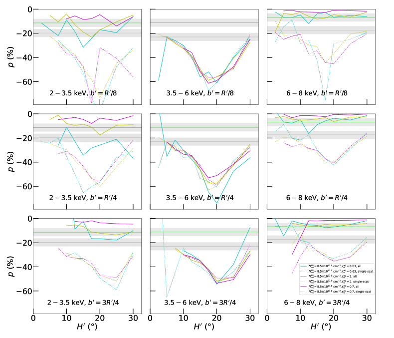
Figure 5.6: The same as in Figure 5.5, but for lower ionization levels. For the highest density case $N_{\textrm{He}}^{\textrm{eq}}=8.5\times 10^{23.0}\ \textrm{cm}^{-2}$ we show $\tau_{\textrm{e}}^{\textrm{eq}}=2$ (yellow) and $\tau_{\textrm{e}}^{\textrm{eq}}=0.7$ (magenta). For the moderate density case $N_{\textrm{He}}^{\textrm{eq}}=8.5\times 10^{22.5}\ \textrm{cm}^{-2}$ we show $\tau_{\textrm{e}}^{\textrm{eq}}=0.63$ (cyan). Image adapted from Podgorný et al. (2023c).

We prove that the single-scattering regime well represents the full model in 3.5–6 keV where no spectral lines are present, which supports the choice of the leading model in Veledina et al. (2023b). Although the conditions to determine the exact level of depolarisation in spectral lines with respect to the continuum can be complex, we obtain a noticeable depolarisation in the 2–3.5 keV and 6–8 keV bands with respect to 3.5–6 keV. The stronger depolarisation by fluorescent lines is more likely for lower ionization fraction.

Apart from the lines, also the energy-dependence of bound-free and free-free absorption affects the energy-dependence of resulting polarisation, which is inherently linked to the geometrical parameters of the system. The only case where the single-scattering approximation does not match the full result in 3.5–6 keV is when low densities and low ionization are in the game (red lines in Figure 5.5). In this case, the depolarisation in continuum energies is too strong due to extended angular distribution of individual scattering events. The depolarisation through changing $N_{\textrm{He}}^{\textrm{eq}}$ is sensitive with respect to the Compton-thickness energy transition, which occurs in or near the 2–8 keV band.

A smaller decrease (increase actually in some low $N_{\textrm{He}}^{\textrm{eq}}$ examples) of polarisation fraction from 3.5–6 keV to 2–3.5 keV is obtained than from 3.5–6 keV to 6–8 keV. The reason is the obscuring medium being indeed more transparent at higher energies, which causes monotonic decrease of polarisation with energy (see Figure 4.3), unlike the depolarisation due to spectral lines, which occurs in the upper and lower energy bin simultaneously. This could possibly explain the leveling of polarisation in the ToO observation detected in 2–6 keV band (Veledina et al., 2023b), compared to the main observation, if the interpretation of decreased density of the obscurer between the two observational periods was correct. We remind, however, that we still derive conclusions from polarisation arising from uniform density of the outflows and a simplistic partial ionization treatment affecting the soft X-rays, which may be critical assumptions difficult to test without further modeling efforts.

5.2 Accreting supermassive black holes

The state-of-the-art scientific advancements in X-ray polarimetry of XRBs slightly turned the topical direction of this dissertation. But since AGNs were originally the primary assignment, forming the title of this work, let us turn our attention back to these objects from observational perspective, as of late 2023. We contributed to the core IXPE team analyses that are mentioned below with source-specific simulations, knowing the parameters of individual sources from literature, similarly to the general investigations described in Chapter 4. Apart from that, we also attempted for a broad observational perspective of AGNs with IXPE and eXTP, as of 2023, to which we devote two specific sections here in the end.

The first observed AGN by IXPE was the type-1 MCG 05-23-16 ($<3.2\%$ in 2–8 keV at a $99\%$ confidence level, Marinucci et al., 2022; Tagliacozzo et al., 2023), observed in two operational windows in May 2022 and November 2022. X-ray stability of the source allowed to add the two sets of observations. The obtained upper limit can still constrain a lot on the inner coronal geometries and many cases of e.g. lamp-post or conical on-axis coronae were disfavored in case of MCG 05-23-16. Similar unobscured and very bright AGN is IC 4329A ($3.3\%\pm 1.9\%$ in 2–8 keV at a $90\%$ confidence level, Pal et al., 2023; Ingram et al., 2023b), observed in March 2023, which allowed to evaluate the polarisation angle as aligned with the colimated large-scale radio ejecta (Unger et al., 1987). It is argued in Ingram et al. (2023b) that the data favor more asymmetric coronae (perhaps outflowing) with elongated direction in the disc plane. Similar geometrical conclusions for the corona were derived for the December 2022 observations of NGC 4151 ($4.9\%\pm 1.1\%$ in 2–8 keV at a $68\%$ confidence level, Gianolli et al., 2023), where the reflection from distant parsec-scale components, however, complicated the spectropolarimetric disentangling. The detected X-ray polarisation in NGC 4151 was aligned with the direction of extended radio emission (Harrison et al., 1986; Ulvestad et al., 1998).

Last but not least, the brightest type-2 AGN, the Circinus Galaxy ($20.0\%\pm 3.8\%$ in 2–6 keV at a $68\%$ confidence level, Ursini et al., 2023b), was observed in July 2022, showing remarkably high X-ray polarisation. As we already mentioned, similar polarisation interpretation to the Cygnus X-3 Galactic black hole was put forward in Ursini et al. (2023b) due to the pure reflection appearance of its spectra and polarisation orientation perpendicular to the projected radio jet (Elmouttie et al., 1998; Curran et al., 2008). We will elaborate below on the limits of such conclusions.

Section 4.3 was devoted to a 3-component toy-model of a full AGN emission that was developed based on the KYNSTOKES central emission model introduced in Section 3.1 and based on previous modeling efforts of parsec-scale components discussed in Marin et al. (2018a, b) and Section 4.1. Although the parameter space covered by this model in Section 4.3 was certainly not complete, we will finish this chapter by providing general polarisation observational prospects in mid X-rays (2–8 keV) for all of the simulation cases studied in Section 4.3. Such analysis is meant to provide rough ideas on how sensitive the contemporary instruments are with respect to a typical sample of AGNs. Contrary to the handful of sources that were already observed by IXPE and that were selected within the mission’s targeting strategy, because they had the highest likelihood for X-ray polarisation detection, according to the literature.

We will use the observation simulation software IXPEOBSSIM (version 30.2.1, Baldini et al., 2022) created for the IXPE mission, which allows to insert unfolded models (such as those from Section 4.3) and provide simulated data and the $M\!D\!P_{99\%}$ in a user-selected energy binning, using the latest IXPE instrumental response matrices (version 12). Given the similarity of instruments on board of the planned eXTP mission, the results for approximately four times lower observational times may be used for observational planning with eXTP, given its larger planned effective mirror area and higher planned sensitivity compared to IXPE (Zhang et al., 2019a). But even for IXPE, the obtained numbers should serve as first-order predictions only, because we will only compare the unfolded model averaged in 2–8 keV to the simulated $M\!D\!P_{99\%}$. And because in the current state, IXPEOBSSIM does not allow to use the weighted analysis, which could additionally lower the $M\!D\!P_{99\%}$ by even $10\%$ (Baldini et al., 2022; Di Marco et al., 2022).

We will begin with the type-1 AGNs studied in Section 4.3, alongside briefly mentioning results for a bare AGN (with no equatorial and no polar scatterers), which the plain KYNSTOKES model described in Chapter 3 can predict. We will finish with general predictions for the type-2 AGNs studied in Section 4.3 with some remarks to the already performed IXPE observation of the Circinus Galaxy. We will keep the positive and negative polarisation degree notation for the rest of this chapter, as our full AGN modeling results (from Section 4.3) that we will primarily work with produce either parallel or perpendicular net polarisation, respectively.

5.2.1 General observational prospects for type-1 active galactic nuclei

Figure 5.8 shows an example of simulated $M\!D\!P_{99\%}$ values in 2–8 keV for one case of type-1 AGN models as input and for a range of single-exposure observation times $T_{\mathrm{obs}}$ and X-ray source fluxes $F_{\mathrm{X,2-10}}$ between 2 and 10 keV. Our simulated 2–8 keV $M\!D\!P_{99\%}$ results are consistent with the values provided in the aforementioned IXPE discovery papers, if the values from unweighted analysis were provided. We display an observational window for IXPE by marking a) the brightest known stable type-1 AGN sources as an upper limit on the $y$-axis ($F_{\mathrm{X,2-10}}\approx 1.8\times 10^{-10}\,\textrm{erg cm}^{-2}\,\textrm{s}^{-1}$, Beckmann et al., 2006; Ingram et al., 2023b) and b) the realistic maximum observational time focused on one source provided by IXPE as an upper limit on the $x$-axis ($T_{\textrm{obs}}\approx 1.5\,\textrm{Ms}\approx 17.4\,\textrm{days}$). If the energy range is further reduced, $M\!D\!P_{99\%}$ typically increases due to the lower number of photons, but see Section 1.2 for details. IXPEOBSSIM allows to adjust the uniformly defined Galactic column density, $N_{\textrm{H}}^{\textrm{gal}}$, which we hold fixed at a generic value of $N_{\textrm{H}}^{\textrm{gal}}=5\times 10^{20}\,\textrm{cm}^{-2}$.

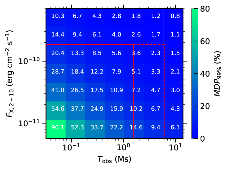
Figure 5.7: An example of the $M\!D\!P_{99\%}$ obtained with IXPEOBSSIM in one 2–8 keV energy bin for various observational times $T_{\textrm{obs}}$ and observed X-ray fluxes $F_{\mathrm{X,2-10}}$ of a type-1 AGN model input with $2\%$ parallelly polarized lamp-post emission, neutral accretion disc extending to the ISCO, black-hole spin $a=1$, absorbing winds of $N_{\textrm{H}}^{\textrm{wind}}=10^{23}\textrm{ cm}^{-2}$ and equatorial torus of $N_{\textrm{H}}^{\textrm{eq}}=10^{24}\textrm{ cm}^{-2}$. The solid red rectangle suggests a somewhat realistic window for an IXPE detection that is on one hand given by the mission’s observational strategy in the point-and-stare regime and on the other hand by the brightest AGNs on the sky. The dashed line shows how the window would approximately enlarge for eXTP in the same energy band, given its planned larger effective mirror area compared to IXPE. Image adapted from Podgorný et al. (2024).

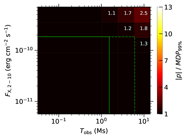
Figure 5.8: The model polarisation degree, $p$, divided by the $M\!D\!P_{99\%}$ obtained with IXPEOBSSIM in one 2–8 keV energy bin for various observational times $T_{\textrm{obs}}$ and observed X-ray fluxes $F_{\mathrm{X,2-10}}$. The polarisation degree is positive in this case. If the ratio of $|p|/M\!D\!P_{99\%}$ is below 1, the polarisation is not detected at the $99\%$ confidence level and we do not display the value and mark the corresponding region in black. The input model is a type-1 AGN with $2\%$ parallelly polarized lamp-post emission, neutral accretion disc extending to the ISCO, black-hole spin $a=1$, absorbing winds of $N_{\textrm{H}}^{\textrm{wind}}=10^{23}\textrm{ cm}^{-2}$ and equatorial torus of $N_{\textrm{H}}^{\textrm{eq}}=10^{24}\textrm{ cm}^{-2}$, i.e. the same as in Figure 5.8. The boundaries in green lines are the same as red lines in Figure 5.8, suggesting a somewhat realistic observational window. Image adapted from Podgorný et al. (2024).

We then plotted for all simulated type-1 AGNs in Section 4.3 the absolute value of the model polarisation degree over the minimum detectable polarisation, $|p|/M\!D\!P_{99\%}$, in the color code (below 1 as black, which means not detectable at a $99\%$ confidence level) versus the same values of $F_{\mathrm{X,2-10}}$ and $T_{\mathrm{obs}}$, as in Figure 5.8. Figure 5.8 shows one such example, which represents one of the most favorable configurations for detection. Rest of the simulated type-1 AGNs required roughly equivalent or higher exposure times or fluxes. We additionally tried linear interpolation of $F_{\mathrm{X,2-10}}$ for three realistic $T_{\mathrm{obs}}$ values and vice versa where $|p|\approx M\!D\!P_{99\%}$, in order to provide rough polarisation detectability clues for a generic set of type-1 sources. The results are provided in Table 4.1, alongside the 2–8 keV polarisation state averages of the underlying model. Although the detectability prospects are not very optimistic on the first look, we note that for some sources multiple observations can be added and, apart from the above mentioned limits of our analysis, X-ray polarisation in certain type-1 AGNs has already been discovered by IXPE, including clues on the properties of their inner-accreting regions (Gianolli et al., 2023; Ingram et al., 2023b). And we note that even an upper limit on polarisation can constrain a non-negligible part of the parameter space (Marinucci et al., 2022; Tagliacozzo et al., 2023). Also in some cases (e.g. Ursini et al., 2023b), IXPE already proved to detect polarisation with greater statistical confidence in a reduced energy range, rather than in the full 2–8 keV band that we examine here only.

From the point of view of highest probability of detection with respect to the studied parameters of the inner-accreting regions, such as the inclination of the observer with respect to the accretion disc, we also tried to examine the case of no equatorial and no polar scatterers. Table 5.1 provides the average total polarisation in 2–8 keV (IXPE and eXTP) and 15–80 keV (XL-Calibur) obtained with the KYNSTOKES model presented in Chapter 3 in the lamp-post and extended sandwich corona regimes for a range of parameter values. When running the same IXPEOBSSIM analysis for the raw KYNSTOKES outputs in the lamp-post regime, only an extremely limited part of the tested parameter region produced detectable polarisation at the $99\%$ confidence level in the same estimated window for type-1 AGNs. The inclination of the accretion disc would have to be close to $\theta=60^{\circ}$, i.e. near the grazing angles for AGN obscuration by dusty tori, and it would have to hold either a highly ionized disc (i.e. with high coronal luminosity and/or low black-hole mass) or a highly polarized primary (with $p_{0}\gtrapprox 3\%$). This holds for nearly any realistic central black-hole spins and lamp-post heights, which are unlikely to be constrained through present-day X-ray polarimetry even in the most favorable scenarios inside the lamp-post geometry concept. Given the low total polarisation degree results for the extended corona with KYNSTOKES presented in Section 3.2 and the 2–8 keV averaged results compared to the lamp-post regime (note that the provided values in Table 5.1 are for unpolarized primary only), we have not even tried the IXPEOBSSIM simulations for the extended coronal version. We note, however, that our central disc-corona model is extremely simplistic and more realistic slab coronal models provide high (a few %) polarisation predictions, especially for high inclinations (Poutanen and Svensson, 1996; Zhang et al., 2019b; Krawczynski and Beheshtipour, 2022; Krawczynski et al., 2022). It would be thus worth to test those coronal models in the same manner, which was outside of scope of this work. Moreover, the first sample of IXPE observations of accreting black holes already resulted in a preference for a corona extending in the accretion disc plane, or left the question of coronal geometry unanswered.

Table 5.1: The unfolded average total polarisation degree, $p\,[\%]$, between 2–8 keV (the IXPE or eXTP mission range) and 15–80 keV (the XL-Calibur balloon experiment range) for unpolarized primary radiation and $\Gamma=2$, as obtained with the KYNSTOKES code described in Chapter 3. We show cases of neutral disc ($M=1\times 10^{8}\,M_{\odot}$ and observed 2–10 keV flux $L_{\textrm{X}}/L_{\textrm{Edd}}=0.001$, left cells in black) and highly ionized disc ($M=1\times 10^{5}\,M_{\odot}$ and observed 2–10 keV flux $L_{\textrm{X}}/L_{\textrm{Edd}}=0.1$, right cells in red) and various combinations of lamp-post heights $h$ (in the lamp-post regime) or radial emissivity power-law indices $q$ (in the extended sandwich corona regime), black-hole spins $a$ and disc inclinations $\theta$. We preserve the notation of the positive and negative polarisation degree, if the corresponding angle is parallel or perpendicular to the projected rotation axis, respectively. We note, however, that due to GR effects the resulting polarisation angle can be off the true main orthogonal directions by even $\approx 20^{\circ}$ (see Chapter 3).

			IXPE and eXTP (2–8 keV)						XL-Calibur (15–80 keV)
			$\theta=30^{\circ}$		$\theta=60^{\circ}$		$\theta=80^{\circ}$		$\theta=30^{\circ}$		$\theta=60^{\circ}$		$\theta=80^{\circ}$
		$a=0$	0.34	2.18	1.04	7.51	1.04	8.46	2.29	2.47	7.48	8.24	7.95	9.04
	$h=3\textrm{ }r_{\textrm{g}}$	$a=1$	0.54	2.13	2.07	6.58	1.03	4.02	2.50	2.61	7.77	7.87	4.66	4.68
		$a=0$	0.24	1.77	0.62	4.97	0.44	3.51	2.03	2.22	5.45	6.07	4.00	4.58
lamp-post corona	$h=15\textrm{ }r_{\textrm{g}}$	$a=1$	0.24	1.72	0.59	4.58	0.37	2.56	1.98	2.17	5.12	5.68	3.26	3.68
		$a=0$	-0.06	-0.01	-0.19	0.01	-0.25	0.04	-0.13	-0.08	-0.44	-0.20	-0.49	-0.11
	$q=3.0$	$a=1$	-0.04	-0.00	-0.11	0.00	-0.14	0.02	-0.08	-0.05	-0.27	-0.12	-0.38	-0.08
		$a=0$	-0.07	-0.01	-0.24	0.02	-0.30	0.06	-0.21	-0.02	-0.55	-0.24	-0.42	-0.07
sandwich corona	$q=1.5$	$a=1$	-0.07	-0.01	-0.24	0.02	-0.28	0.02	-0.21	-0.12	-0.53	-0.24	-0.42	-0.08

5.2.2 General observational prospects for type-2 active galactic nuclei and analysis of the Circinus Galaxy IXPE observations

We performed the same IXPEOBSSIM simulations with the type-2 AGN synthetic spectra and polarisation from Section 4.3 as inputs. Comparing to type-1 AGNs, here the situation is more favorable in high polarisation degree expected in the IXPE band. But as usual, high polarisation through more specific geometry of scattering (a reduced symmetry) is to the detriment of average expected photon count rate. The brightest type-2 AGNs are detected in X-ray fluxes at least an order of magnitude lower ($F_{\mathrm{X,2-10}}\approx 1.5\times 10^{-11}\,\textrm{erg cm}^{-2}\,\textrm{s}^{-1}$, Bianchi et al., 2002; Tanimoto et al., 2022). We mark this value along with the same maximum $T_{\mathrm{obs}}$ in Figure 5.9 that shows the same heatmaps of $|p|/M\!D\!P_{99\%}$ versus $F_{\mathrm{X,2-10}}$ and $T_{\mathrm{obs}}$ for the type-2 cases with absorbing winds, ionized winds and no winds for three different torus column densities and one set of parameter values related to the nucleus. In the provided numbers on each heatmap, we keep the sign of $p$, i.e. we note the values of $p/M\!D\!P_{99\%}$, because for type-2 AGNs the resulting polarisation angle can be either parallel or orthogonal to the principal axis. The underlying average 2–8 keV unfolded model polarisation values were provided in Table 4.2 already, alongside the same linear interpolation results for three values of $F_{\mathrm{X,2-10}}$ and $T_{\mathrm{obs}}$ where $|p|\approx M\!D\!P_{99\%}$, as in Table 4.1. The wide conclusions are similar to the type-1 AGNs: although the first AGN observations by IXPE proved that for the brightest and well-known sources the X-ray polarisation data can improve our knowledge significantly, the complexity and diversity of AGNs (especially of the parsec-scale components with respect to type-2 AGNs) is preventing us from providing a clear diagnostic tool or a qualitative guidance for a general set of sources, given the contemporary sensitivity of X-ray polarimetric instruments. Such goals are too ambitious for the near future. Regarding the prospects for plain detectability by IXPE or eXTP with respect to faintness of AGNs, the situation is perhaps more favorable towards type-2 sources rather than towards unobscured AGNs.

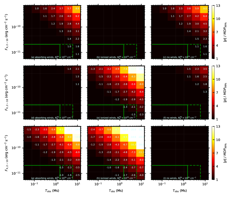
Figure 5.9: The same as in Figure 5.8, but the input model is a type-2 AGN with $2\%$ parallelly polarized lamp-post emission, neutral accretion disc extending to the ISCO, black-hole spin $a=1$. We show nine different configurations of the parsec-scale components: (a) absorbing winds of $N_{\textrm{H}}^{\textrm{wind}}=10^{21}\textrm{ cm}^{-2}$ and equatorial torus of $N_{\textrm{H}}^{\textrm{eq}}=10^{23}\textrm{ cm}^{-2}$ (top-left), (b) ionized winds and equatorial torus of $N_{\textrm{H}}^{\textrm{eq}}=10^{23}\textrm{ cm}^{-2}$ (top-middle), (c) no winds and equatorial torus of $N_{\textrm{H}}^{\textrm{eq}}=10^{23}\textrm{ cm}^{-2}$ (top-right), (d) absorbing winds of $N_{\textrm{H}}^{\textrm{wind}}=10^{21}\textrm{ cm}^{-2}$ and equatorial torus of $N_{\textrm{H}}^{\textrm{eq}}=10^{24}\textrm{ cm}^{-2}$ (middle-left), (e) ionized winds and equatorial torus of $N_{\textrm{H}}^{\textrm{eq}}=10^{24}\textrm{ cm}^{-2}$ (center), (f) no winds and equatorial torus of $N_{\textrm{H}}^{\textrm{eq}}=10^{24}\textrm{ cm}^{-2}$ (middle-right), (g) absorbing winds of $N_{\textrm{H}}^{\textrm{wind}}=10^{21}\textrm{ cm}^{-2}$ and equatorial torus of $N_{\textrm{H}}^{\textrm{eq}}=10^{25}\textrm{ cm}^{-2}$ (bottom-left), (h) ionized winds and equatorial torus of $N_{\textrm{H}}^{\textrm{eq}}=10^{25}\textrm{ cm}^{-2}$ (bottom-middle), (i) no winds and equatorial torus of $N_{\textrm{H}}^{\textrm{eq}}=10^{25}\textrm{ cm}^{-2}$ (bottom-right). The negative sign in front of the written values in some panels indicates that in this case, the net model polarisation angle in 2–8 keV is orthogonal to the projected system axis of symmetry. In the color code, we keep the absolute value of polarisation degree for consistency of polarisation detectability estimates with other cases. The solid green rectangle again suggests a somewhat realistic window for an IXPE detection that is on one hand given by the mission’s observational strategy in the point-and-stare regime and on the other hand by the brightest type-2 AGNs on the sky. The dashed line shows how the window would enlarge for eXTP in the same energy band, given its planned larger effective mirror area compared to IXPE. Image adapted from Podgorný et al. (2024).

In the case of absorbing winds, the higher the equatorial obscuration is, the higher the contribution from the perpendicularly polarized component we obtain in the 2–8 keV band over the parallel polarisation that is more likely arising from the equatorial scatterings. However, the flux has a reverse dependency on the torus thickness due to absorption. The dependency of such trade-off in X-ray polarisation detectability on the torus density is interesting with regards to 2–8 keV $M\!D\!P_{99\%}$ for IXPE. We obtain higher probability of 2–8 keV detection for tori with $N_{\textrm{H}}^{\textrm{eq}}=10^{23}\textrm{ cm}^{-2}$ than for tori with $N_{\textrm{H}}^{\textrm{eq}}=10^{24}\textrm{ cm}^{-2}$. However, the cases with $N_{\textrm{H}}^{\textrm{eq}}=10^{25}\textrm{ cm}^{-2}$ show again better observational prospects than for $N_{\textrm{H}}^{\textrm{eq}}=10^{24}\textrm{ cm}^{-2}$, in fact the most promising out of the three examples. In order to explain this behavior, we will first analyze the other cases of polar winds, because their compositions plays an important role.

In the case of ionized winds, we get low polarisation detection probabilities for low torus column density of $N_{\textrm{H}}^{\textrm{eq}}=10^{23}\textrm{ cm}^{-2}$. The situation is significantly more promising towards detections for $N_{\textrm{H}}^{\textrm{eq}}=10^{24}\textrm{ cm}^{-2}$ and even more for $N_{\textrm{H}}^{\textrm{eq}}=10^{25}\textrm{ cm}^{-2}$. For the case with the lowest torus transparency, we obtain higher detectability for ionized winds compared to the absorbing winds. This is because for the ionized winds, we place an ideal polar reflector (causing high $\gtrapprox 25\%$ perpendicularly oriented polarisation) for photons emerging upwards and reaching the observer through the “periscope”. In the case of no polar winds, we get a reverse dependency of detectability with equatorial torus thickness. We obtain better observational conditions, if the torus is more transparent, which in addition to higher flux produces higher average 2–8 keV polarisation with parallel orientation (see Table 5.9). Hence, the case of absorbing case produces an intermediate case, mixing these two effects. This is clear from the expected 2–8 keV polarisation angle that changes by $90^{\circ}$ between $N_{\textrm{H}}^{\textrm{eq}}=10^{23}\textrm{ cm}^{-2}$ and $N_{\textrm{H}}^{\textrm{eq}}=10^{25}\textrm{ cm}^{-2}$. For the former case the delicate energy transition between the two polarisation states seen in the simulations (discussed in Section 4.3) occurs at energies rather lower from the IXPE band. Although in the analysis presented here, the 2–8 keV detectability results are in addition related to the energy-dependent flux.

Such discussion is worth applying to the so-far only observed type-2 AGN by IXPE: the Circinus Galaxy (with Compton thickness $N_{\textrm{H}}>10^{24}\textrm{ cm}^{-2}$, Arévalo et al., 2014; Kayal et al., 2023), described and interpreted in Ursini et al. (2023b). The study provides a detailed spectropolarimetric analysis that suggests that the observed polarisation of $17.6\%\pm 3.2\%$ in the 2–8 keV band (at $68\%$ confidence level) can be largely attributed to the equatorial scatterings, while the polarisation from the polar reflection is claimed unconstrained. They assumed two distinct power-law indices $\Gamma=1.6$ and $\Gamma=3.0$ for the cold (equatorial) and warm (polar) reflectors, respectively, that were kept fixed in the spectropolarimetric fit, which resulted in low total flux contribution of the warm reflector, thus low contribution to the net polarisation. If different assumptions were taken more in favor of the warm reflector, it could affect the result of the polarisation component analysis.

Thus, given our models that in addition include the polar reflector (compared to Ursini et al., 2023b, where only the equatorial scattering region is considered), we humbly propose reconsideration of the contribution to the polarisation detected in the Circinus Galaxy by IXPE that could be on the other hand almost entirely attributed to the partly ionized polar scattering region. This is supported furthermore by the fact that our simulations from Section 4.3 and those in Marin et al. (2018b) clearly lead to two contributions to the net polarisation state that are distinguished by a $90\mbox{${}^{\circ}$}$ switch in the polarisation angle. The observed polarisation in the Circinus Galaxy is orthogonal to the principal axis of the entire accreting system (Ursini et al., 2023b). Hence, this orientation is consistent with our interpretation for polar scatterings, on average symmetric in the meridional plane. When studying the equatorial parsec-scale scattering regions in detail in Section 4.1, we argued that the parallelly oriented summed polarisation vector is more likely to arise from equatorial reprocessings, if the half-opening and the observer’s inclination are high enough, which is the case of Circinus Galaxy (Kayal et al., 2023). In such cases, the equatorial component may rather serve as a depolarizer and dilutes the orthogonally and highly polarized warm reflection from the poles.

When considering the expected and observed energy dependence of polarisation in Circinus Galaxy, the above conclusions are also supported. Although it is beyond the scope of this work to examine combinations of different energy binnings in 2–8 keV range in detail, we clearly see that the simulations result in high (tens of %) polarisation with perpendicular orientation at soft X-rays, thanks to the polar scatterer. This component then prevails more inside (or even above) the 2–8 keV band for higher column densities of the torus. In Ursini et al. (2023b), it is proposed that the non-detection of polarisation in 6–8 keV is due to the presence of unpolarized iron line, which is certainly true. However, it suggests itself that an additional effect of depolarisation in 6–8 keV can be due to the competing polarisation contribution in parallel direction with respect to the principal axis arising from the equatorial reprocessings. For high enough Compton thickness of the dusty torus that the source is likely possessing (Arévalo et al., 2014; Kayal et al., 2023) this would not mean a switch of the polarisation angle to parallel orientation at higher energies within the 2–8 keV band, which is indeed not observed (Ursini et al., 2023b), but only a dilution of polarisation with the same orientation. The switch would occur at even higher energies due to the reduced flux contribution from light passing directly through the opaque torus (see Section 4.3 and Marin et al., 2018b).

Chapter 6 Conclusions and future prospects

Let us conclude and provide directions of useful continuation of this work. In the beginning, we promised that we will show how elementary geometrical principles may be used to derive information on the outer space. We argued that in the case of AGNs and XRBs, the (a)symmetry in the origin of X-ray emission yields polarisation signatures in the observed electromagnetic radiation, as the preferred orientation of the electric vector position angle is determined by the emission and reprocessing mechanisms, as well as superposition effects. In this way, any broken spatial symmetry in the interaction of light and matter inside the system, from quantum Planck scales all the way to multiples of black-hole radii where gravity matters, may lead to enhanced net polarisation in a beam of photons on behalf of the naturally randomly polarized (unpolarized) light. In the X-rays near accreting black holes, this is associated mostly with magnetic fields, scattering and absorption mechanisms, as the main physical drivers of X-ray polarisation modifications. We restricted ourselves to configurations where magnetic fields do not intervene significantly in the X-ray emission. We assumed a given background gravity field and matter configuration according to known information on AGNs and XRBs, which comes from the interplay of observations and logical deduction based on elementary conservation principles and known fundamental interactions.

Devoting the first half of our results to theory, we developed a series of X-ray spectropolarimetric numerical models from local radiative transfer computations applied to photospheres of accretion discs, to estimators of strong-gravity effects on the emergent light near the black-hole event horizon, to models of reprocessing in distant circumnuclear components. By constructing toy models of reasonable simplifications and assumptions – to the detriment of computational expensiveness and hopefully not much to the detriment of accurate description of physical reality – we provided predictions for X-ray polarimetric observations of AGNs and XRBs. These may serve for analysis of the recent discoveries by the leading X-ray polarimetric mission IXPE, as well as for observational prospects with the current and forthcoming X-ray polarimeters (such as IXPE, XL-Calibur – already launched –, or eXTP – planned to be launched in 2027). Despite being largely degenerated in the considered parameter space with respect to predicted X-ray polarisation, the models may result in significantly more informative potential, if combined with X-ray spectroscopic and timing techniques, or polarimetry of AGNs and XRBs at other wavelengths. The power of observational X-ray polarimetry in multi-wavelength and multi-instrument campaigns was demonstrated in the last part of the results where many recent IXPE results were presented, alongside direct applications of the numerical models developed in the first part of this work.

In Chapter 2 we presented a calculation for arbitrarily polarized X-ray power-laws reprocessed in constant-density disc atmospheres, comoving with the source of irradiation. We used an iterative radiative transfer equation solver TITAN and a MC simulator STOKES, aiming at polarisation estimation with high accuracy and developing models, primarily for AGNs. Both X-ray spectroscopy and X-ray polarimetry are powerful independent methods to derive the spin of the central accreting black hole (not only) by means of reflected coronal radiation from inner regions of the accretion discs. High-fidelity reflection modeling is, however, necessary to infer information not only on the black-hole spin, but also on the system inclination and orientation, as well as on the accretion disc’s properties and ionization structure. We showed that careful treatment of partial ionization of the disc’s upper layers is critical for the resulting X-ray polarisation profiles with energy.

We may improve the presented model in several ways. In the future, it would be beneficial to release the assumption of constant density, as this is expected to have an impact on both the resulting spectra and polarisation (e.g. Różańska et al., 2002; Ross and Fabian, 2007; Różańska et al., 2011; Podgorný et al., 2022). This would, however, require designing a completely new setup. Minor improvements and checks for model dependencies of the results are achievable with less effort. Apart from addressing different cut-off selections or cosmic matter abundances, adding more spectral lines, or attempting for pencil-like illumination in TITAN, perhaps the easiest first step towards generalization would be attempting for the same computations, just for different slab densities. High-density reflection tables, suitable for accretion discs of XRBs, can be compared in their spectral part much in the same way to the high-density XILLVER (García et al., 2016) and REFLIONX (the REFHIDEN version of the standard tables Ross and Fabian, 2005, 2007) tables. Cross-validation at a deeper level in flux is necessary for assessing polarisation properties of this flux in reflecting high-density disc models.

We argued that with contemporary numerical facilities it is difficult to derive information on the inner-accreting structures in the vicinity of black holes from X-ray polarimetry of thermally emitting disc atmospheres. Due to the expected accretion disc X-ray properties, here the main applications are for XRBs, rather than AGNs. With the same codes and major assumptions as for the reflection studies, we constructed models of passive scattering and absorbing layers in transmission, illuminated from the opposite side by isotropic single-temperature black-body radiation, representing the radiative power input from a significantly heated optically thick accretion disc below. The absorbing medium may cause substantial flux depletion in the transmitted radiation at about 3 keV, which results in rather high and decreasing polarisation degree with energy between 2–8 keV where IXPE operates. However, if the plane-parallel slab is ionized enough, which is a natural state of the tested plane-parallel slabs in photo-ionization equilibrium, the X-ray spectropolarimetric properties of the emergent radiation do not change significantly with further ionization by decrease of medium density or increase in irradiating intensity. Alongside typical X-ray signatures of high ionization in XRBs in the thermal state, the obtained model polarisation degree with energy, which is constant or increasing in 2–8 keV, may be used to explain some puzzling IXPE observations of XRBs in the high/soft state (namely 4U1630-47 and LMC X-3, Ratheesh et al., 2024; Svoboda et al., 2024), by means of enhanced absorption and Compton down-scattering effects and possibly by adding outflowing velocities to the absorbing and scattering medium that cause additional polarisation increase due to aberration. In such high ionization limit, however, the disc structure and the absorption and scattering geometry is largely unconstrained by our model.

It would be useful to put more effort in constructing full semi-infinite atmosphere models in X-ray polarisation gained by transmission of thermal radiation, which so far consist of only few examples in the literature. A few more individual and brave attempts in detailed radiative transfer modeling – without the ambitions for constructing a data-fitting tool – can tell a lot in favoring or disfavoring of an entire class of less sophisticated theoretical works, which are typically more useful for direct data fitting. Although the model that was presented in this dissertation fails at high slab thickness, there are possibilities of adaptation. The TITAN code allows for boundary conditions that could be used for thick atmospheres and using the information from TITAN on the source function through intermediate layers in the non-LTE conditions (after convergence of the iterative ALI computations), we could compensate for the flux loss, which is inevitable in the MC STOKES results for thick atmospheres. In a broader view, different illuminating spectra or combined illumination (most importantly the same slab seen in transmission for a black body and in reflection for a power-law: with the vertical ionization structure consistently precomputed) are also accessible, since we have well tested the two detached illumination examples already, using the same method with TITAN and STOKES. Another critical update of this part of work on local spectropolarimetric radiative transfer would be to use the latest STOKES v2.34 version that includes Comptonization effects, which should be tested first with the already performed models to track changes in the results, as we neglected inverse Compton scattering in this work.

Apart from the ongoing IXPE campaigns, much progress in our understanding of XRBs in the soft state is also expected from future (non-)detections of polarisation in other X-ray energy bands. Such as in the 15–80 keV window that is covered by the XL-Calibur experiment and that can reveal more on the continuation of the rise of polarisation with energy in 2–8 keV, which is currently detected in many XRBs. Observing new sources with IXPE with known projected orientation on the sky would also help to validate the above presented modeling directions, because our model of thermal emission passing through an absorbing atmosphere is valid only if the resulting polarisation angle is parallel to the prevailing slab plane, similarly to most of the decades old analytical results. If the polarisation directions orthogonal to the disc plane become observationally preferred for thermal emission in the near future, either a delicate combination of optically thin covering medium with particular distribution of internal sources, or geometries, or bulk motions would have to be assumed, or perhaps this would be exactly a small example in the history of science where a new gate opens and we might be missing something fundamental. Observing the same sources again and observing new sources with IXPE would both help in this sense.

In Chapter 3, we provided two relativistic models of the entire disc-corona system: assuming the lamp-post geometry and the sandwich slab geometry. They incorporate the local reflection tables for partially ionized AGN accretion discs discussed in Chapter 2 and provide first-order estimates of major quantities describing the inner-accreting regions via spectropolarimetric fitting in XSPEC or by means of unfolded model comparison. Focusing on X-ray polarisation arising from reflection, we discussed the major spectropolarimetric properties of these regions. The predicted X-ray polarisation fraction gained by reflection from geometrically thin accretion discs extending to the ISCO in the lamp-post models is typically increasing with energy, of the order of a few %, and with a polarisation angle oriented parallel to the principal axis. In most of the tested scenarios, the X-ray polarisation obtained from reflection in accretion discs in the sandwich slab coronal models is less than $1\%$, peaking in the IXPE band and with polarisation angle typically parallel to the equatorial plane. In addition, KYNSTOKES allows to assess the inner disc radius location through X-ray polarisation by reflection. In the lamp-post geometries, the polarisation gain by geometrical reduction is to the detriment of flux in the reflected component. Such diagnostics may be useful again towards the upcoming bright times of observational X-ray polarimetry and towards our understandings of the accretion mechanisms.

Regarding future development of the relativistic codes presented here, it is highly desirable to reimplement any newer version of the local reflection tables, especially towards any models more suitable for XRBs. Then, we need to release the isotropic emission assumption of the lamp-post corona or function with more realistic coronal emission by implementing the standard disc reflection from KYNSTOKES for arbitrary input into MONK or KerrC. Studying different coronal properties in this way provides much room for new discoveries.

Departures from the Kerr metric are not possible to test with our models, but could be critical. Returning radiation effects in Kerr spacetime for X-ray polarisation by disc reflection need to be thoroughly investigated already in the scope current models, as the recent spectral analysis of returning radiation in Dauser et al. (2022) suggests that they could play a role.

Apart from KYNSTOKES that studies reflection from a geometrically thin disc, we may also try to implement the new local reflection tables to the SLIMBH model, built for slim discs, as these are in many theoretical and observational arguments preferred over the standard Novikov-Thorne accretion. The work of West and Krawczynski (2023) is currently also taking lead in assessing the critical assumption of the disc thickness, including full GR treatment.

In Chapter 4, we provided a set of computations assessing X-ray polarisation properties of distant circumnuclear components. These are far enough from the core, to be separated from GR effects that affect the source radiation near its origin and complicate the modeling. However, the reprocessed polarisation is still highly dependent on the composition, shape and size of the scattering regions. In case of both AGNs and XRBs, this is more important for X-ray polarimetry of obscured sources, viewed rather edge-on. Rather than attempting for providing clear guidelines for observational analysis, which is too ambitous in the current state of knowledge, we argued that even with static and homogeneous toroidal equatorial obscurers, the diversity in possible X-ray polarisation production of the reprocessed signal is striking, reaching tens of % in parallel or perpendicular orientation with respect to the axis of symmetry.

By means of comparing the detailed MC simulations with STOKES to a simplified model of reflection from the inner toroidal surface, we showed that large part of the diversity in X-ray polarisation is due to geometry of the reprocessing medium only. The newly built simple model and its associated routines open up place for easy-to-implement modifications and for a new class of XSPEC spectropolarimetric models suitable for studying reflection from axially symmetric surfaces without any relativistic effects. However, the remaining differences between the simple approach and a full MC simulation (that accounted for e.g. partial transparency and self-irradiation effects) still proved to be important for the polarisation predictions, modifying the results by at least few % in the testing 3.5–6 keV and 30–60 keV bands towards higher perpendicular polarisation fraction with respect to the axis of symmetry.

We envision that the additional modeling of non-homogeneous distant scattering regions, which we did not do here, is necessary to assess the sensitivity to this assumption. At least the AGN tori are largely believed to be clumpy (Nenkova et al., 2002; Risaliti et al., 2002; Matt et al., 2003; Tristram et al., 2007) and a detailed X-ray polarisation model could be conversely used for examination of the clumpiness characteristics (Marin et al., 2012, 2013, 2015). We also completely ignored possible misalignment of the scattering regions, which would be of scope of another study of the same length, as releasing this assumption opens at least one new dimension in the parameter region (Goosmann and Matt, 2011). Another useful way of continuation of this work would be the study of different irradiating spectral distributions, or non-isotropic or spatially extended sources.

Since the presented modeling represents one of the first broad-parametric attempts for X-ray polarisation estimates from geometrically thick equatorial obscurers, it would be highly beneficial to carry out a detailed comparative study with respect to the simultaneously emerging analytical models (Veledina et al., 2023b) and MC codes (Ghisellini et al., 1994; Ratheesh et al., 2021; Ursini et al., 2023b; Vander Meulen et al., 2023; Tomaru et al., 2024; Tanimoto et al., 2023) in the near future.

In Chapter 5, we provided a few examples of usage of the new numerical models for the interpretation of the first IXPE observations. In addition, we provided general observational prospects for accreting black holes. Not only IXPE, operating in the mid X-rays, and XL-Calibur, operating in the hard X-rays are believed to bring interesting X-ray polarimetric discoveries in the near future. We also mentioned the eXTP mission, which should be a successor of IXPE, operating in the same energy band with about four times larger effective mirror area. The soft X-ray sounding rocket experiment REDSoX, planned to operate in 0.2–0.8 keV, could also reveal a lot of X-ray polarisation mysteries around accreting black holes, given our models. Although in AGNs, the soft X-rays are usually a matter of debates already from the spectroscopic point of view due to the presence of the soft excess in flux, which we have not modelled thoroughly.

Staying humble with the scientific progress that this individual work allowed, we stress the general utility of X-ray polarimetry in the context of high-energy astrophysics that was theoretically envisioned already in the 1970s and now is observationally becoming confirmed. For the case of accreting black holes either by strongly favoring locations of the hot emitting plasma, which are critically unknown inside the accretion flow, much like a microscope providing physical clues to unresolved structures. Or by showing surprises in high X-ray polarisation of unknown origin in the reprocessings of thermal emission, arising from the core. Independent clues to black-hole spin values, which are typically extremely high from X-ray spectroscopy (a surprising outcome for a dynamical evolution), or to the accretion disc’s inclination, size and structure, which are for many sources completely unknown, are only a matter of time when larger samples of X-ray polarimetric observations will be collected. The same holds for characteristics of equatorial and polar outflows and tests of the unification scenario for AGNs, which is dependent on the positioning and composition of parsec-scale components of various kinds that X-ray polarimetry can unravel.

If more observational surprises are yet to come and theoretical efforts lack behind, in such examples, it suggests itself to learn from other branches of astrophysics, such as the solar physics, where observational data as well as numerical simulations are typically more developed than for black-hole environments (e.g. Stenflo, 1994; Landi Degl’Innocenti and Landolfi, 2004; Heinzel et al., 2020). One can also learn from laboratory X-ray polarimetry (e.g. Giles et al., 1995; Huard, 1997; Stöhr and Siegmann, 2006; Grizolli et al., 2016; Shah et al., 2016; Yang et al., 2021; Stöhr, 2023) that solves many quantum phenomena in greater detail than the astrophysical sources allow, despite being unique in the extreme physical conditions that are occurring elsewhere in our Universe.

Appendix A Supplementary material

Supplementary figures to Chapter 2

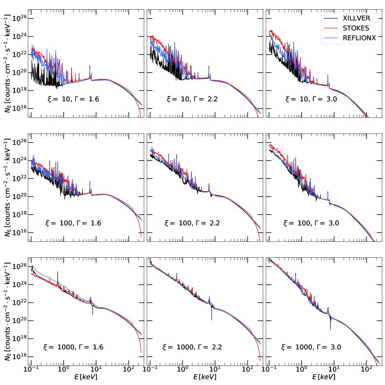
Figure A.1: The same as in Figure 2.3, but for various $\xi$ in $[\textrm{erg}\cdot\textrm{cm}\cdot\textrm{s}^{-1}]$ and $\Gamma$.

Figure A.2: Various cases of transmitted single-temperature unpolarized black-body radiation with $k_{\textrm{B}}T_{\textrm{BB}}=1.15$ keV through a constant density slab, as computed with TITAN and STOKES in PIE. From left to right the flux of the irradiation increases ($\xi=3\times 10^{0},3\times 10^{2},3\times 10^{4},3\times 10^{5},3\times 10^{8}\,\,\textrm{erg}\cdot\textrm{cm}\cdot\textrm{s}^{-1}$, respectively) and the slab is more ionized for the same density $n_{\textrm{H}}=10^{18}\ \textrm{cm}^{-3}$. Top row: fractional abundance of ions of oxygen (blue) OI–OIX and iron (red) FeI–FeXXVII from TITAN ionization structure precomputations. Bottom row: the effective optical depth, $\tau_{\textrm{eff}}$, divided by column density, $N_{\textrm{H}}\,[\textrm{cm}^{-2}]$, versus energy for continuum processes (black) and including lines (cyan) from TITAN ionization structure precomputations. Thomson cross-section $\sigma_{\textrm{T}}$ (yellow) represents pure scatterings.

Figure A.3: The STOKES results for $\tau_{\textrm{T,max}}=1$, corresponding to the cases shown in Figure A.2. From left to right the flux of the irradiation increases ($\xi=3\times 10^{0},3\times 10^{2},3\times 10^{4},3\times 10^{5},3\times 10^{8}\,\,\textrm{erg}\cdot\textrm{cm}\cdot\textrm{s}^{-1}$, respectively) and the slab is more ionized for the same density $n_{\textrm{H}}=10^{18}\ \textrm{cm}^{-3}$. Top row: spectra, $F$, per energy bin for various observer’s inclinations $\theta$ in the color code. Bottom row: the corresponding polarisation degree, $p$, versus energy (solid lines) for various observer’s inclinations $\theta$ in the color code. We indicate the pure-scattering limit for semi-infinite atmosphere given by Chandrasekhar-Sobolev approximation for the same inclination values (dashed horizontal lines). The obtained polarisation angle from STOKES is constant with energy and parallel with the slab.

Supplementary figures to Chapter 3

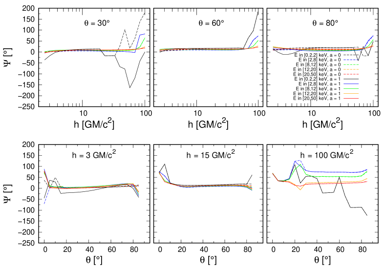
Figure A.4: Top panel: the total average polarisation angle, $\Psi$, versus height of the primary point-source above the disc for disc inclinations $\theta=30^{\circ}$ (left), $\theta=60^{\circ}$ (middle) and $\theta=80^{\circ}$ (right), $\Gamma=2$, unpolarized primary radiation, $M=1\times 10^{8}\,M_{\odot}$ and observed 2–10 keV flux $L_{\textrm{X}}/L_{\textrm{Edd}}=0.001$, i.e. neutral disc. We show cases of two black-hole spins $a=0$ (dashed) and $a=1$ (solid) and for energy bands $E\in[0.2,2]$ keV (black), $E\in[2,8]$ keV (blue), $E\in[8,12]$ keV (green), $E\in[12,20]$ keV (orange), and $E\in[20,50]$ keV (red). Bottom panel: the total average polarisation angle, $\Psi$, versus disc inclination for heights of the primary point-source above the disc $h=3\textrm{ }r_{\textrm{g}}$ (left), $h=15\textrm{ }r_{\textrm{g}}$ (middle) and $h=100\textrm{ }r_{\textrm{g}}$ (right), for the same configuration as on the top panel.

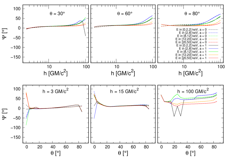
Figure A.5: The total average polarisation angle, $\Psi$, versus energy for ionized disc ($M=1\times 10^{5}\,M_{\odot}$ and observed 2–10 keV flux $L_{\textrm{X}}/L_{\textrm{Edd}}=0.1$), otherwise for the same parametric setup as in Figure A.4, displayed in the same manner.

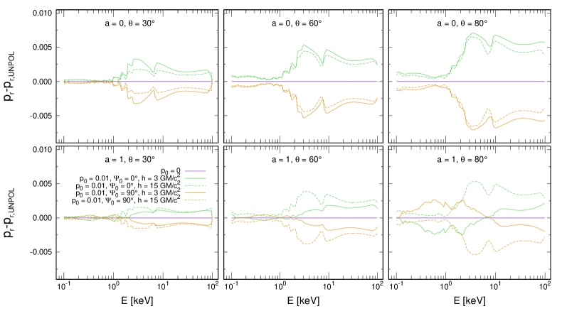
Figure A.6: The relative difference of the reflected-only polarisation degree versus energy of the accretion disc for distant observer from a case with unpolarized primary radiation: $p_{\mathrm{r}}-p_{\mathrm{r,UNPOL}}$, obtained by KYNSTOKES for black-hole spins $a=0$ (top) and $a=1$ (bottom), disc inclinations $\theta=30^{\circ}$ (left), $\theta=60^{\circ}$ (middle) and $\theta=80^{\circ}$ (right), $\Gamma=2$ and neutral disc ($M=1\times 10^{8}\,M_{\odot}$ and observed 2–10 keV flux $L_{\textrm{X}}/L_{\textrm{Edd}}=0.001$), using the STOKES local reflection model in the lamp-post scheme. We show cases of two different heights of the primary point-source above the disc $h=3\textrm{ }r_{\textrm{g}}$ (solid lines) and $h=15\textrm{ }r_{\textrm{g}}$ (dashed lines), and three different polarisation states of the primary source for which $p_{\mathrm{r}}$ was computed: $p_{0}=0$ (purple), $p_{0}=0.01$ and $\Psi_{0}=0^{\circ}$ (green), $p_{0}=0.01$ and $\Psi_{0}=90^{\circ}$ (orange).

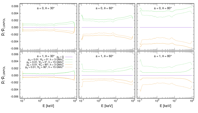
Figure A.7: The reflected-only polarisation degree, $p_{\mathrm{r}}-p_{\mathrm{r,UNPOL}}$, versus energy for highly ionized disc ($M=1\times 10^{5}\,M_{\odot}$ and observed 2–10 keV flux $L_{\textrm{X}}/L_{\textrm{Edd}}=0.1$), otherwise for the same parametric setup as in Figure A.6, displayed in the same manner.

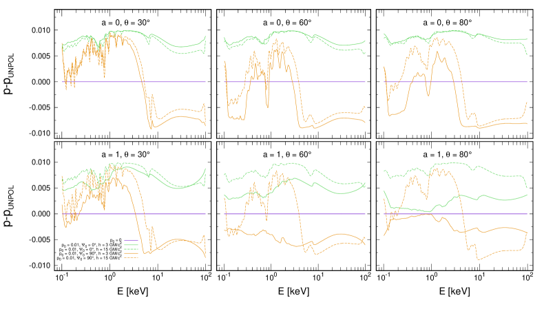
Figure A.8: The total polarisation degree, $p-p_{\mathrm{UNPOL}}$, versus energy for the same parametric setup as in Figure A.6, displayed in the same manner.

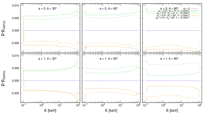
Figure A.9: The total polarisation degree, $p-p_{\mathrm{UNPOL}}$, versus energy for the same parametric setup as in Figure A.7, displayed in the same manner.

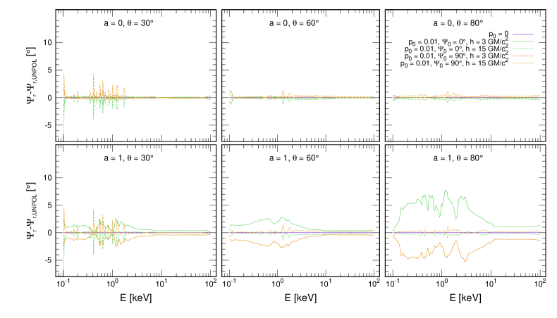
Figure A.10: The reflected-only polarisation angle, $\Psi_{r}-\Psi_{\mathrm{r,UNPOL}}$, versus energy for the same parametric setup as in Figure A.6, displayed in the same manner.

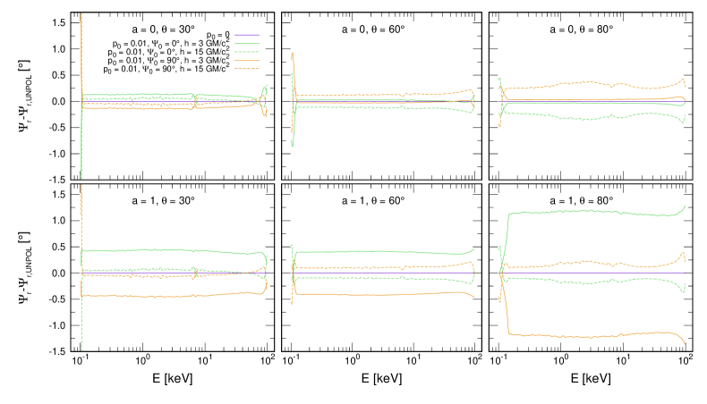
Figure A.11: The reflected-only polarisation angle, $\Psi_{\mathrm{r}}-\Psi_{\mathrm{r,UNPOL}}$, versus energy for highly ionized disc ($M=1\times 10^{5}\,M_{\odot}$ and observed 2–10 keV flux $L_{\textrm{X}}/L_{\textrm{Edd}}=0.1$), otherwise for the same parametric setup as in Figure A.6, displayed in the same manner.

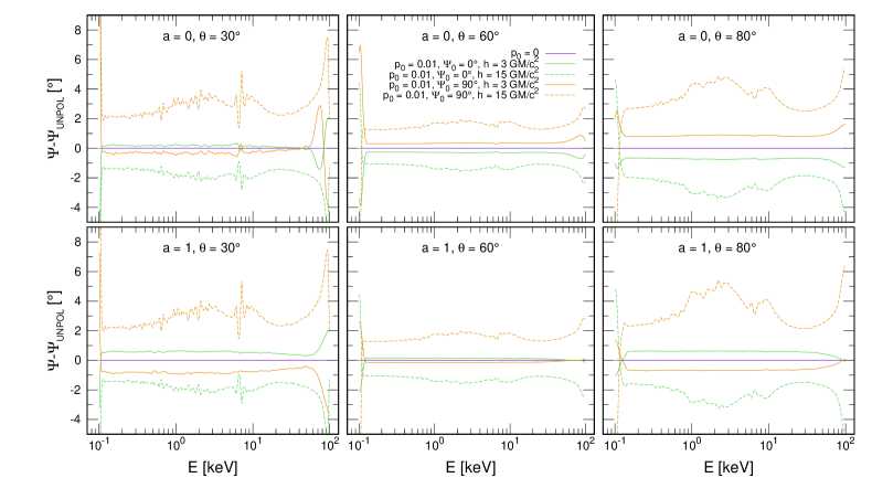
Figure A.12: The total polarisation angle, $\Psi-\Psi_{\mathrm{UNPOL}}$, versus energy for the same parametric setup as in Figure A.11, displayed in the same manner.

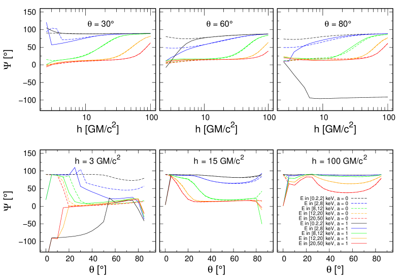
Figure A.13: The total average polarisation angle, $\Psi$, versus energy for primary polarisation of $p_{0}=0.01$ and $\Psi_{0}=90^{\circ}$, otherwise for the same parametric setup as in Figure A.4, displayed in the same manner.

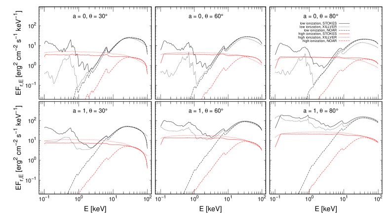
Figure A.14: The reflected-only spectra of the accretion disc for distant observer in the lamp-post scheme, $EF_{\textrm{r,E}}$, for black-hole spins $a=0$ (top) and $a=1$ (bottom), $\theta=30^{\circ}$ (left), $\theta=60^{\circ}$ (middle) and $\theta=80^{\circ}$ (right), $\Gamma=2$, height of the primary point-source above the disc $h=3\textrm{ }r_{\textrm{g}}$ and unpolarized primary radiation. We compare cases of KY disc integration with the STOKES local reflection tables (solid lines), XILLVER local reflection tables (dotted lines) and NOAR local reflection tables (dashed lines), and neutral disc ($M=1\times 10^{8}\,M_{\odot}$ and observed 2–10 keV flux $L_{\textrm{X}}/L_{\textrm{Edd}}=0.001$, black lines) and highly ionized disc ($M=1\times 10^{5}\,M_{\odot}$ and observed 2–10 keV flux $L_{\textrm{X}}/L_{\textrm{Edd}}=0.1$, red lines).

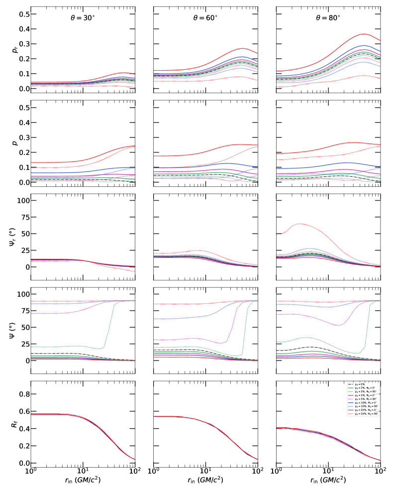
Figure A.15: The same as in Figure 3.11, but for $h=15\textrm{ }r_{\textrm{g}}$.

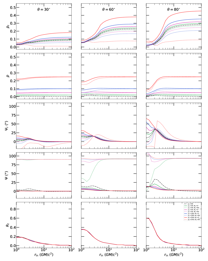
Figure A.16: The same as in Figure 3.11, but for neutral disc.

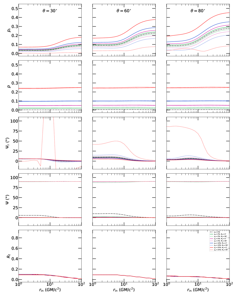
Figure A.17: The same as in Figure 3.11, but for $h=15\textrm{ }r_{\textrm{g}}$ and neutral disc.

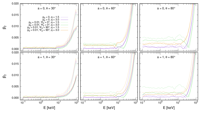
Figure A.18: The reflected-only polarisation degree, $p_{\mathrm{r}}$, versus energy of the accretion disc for a distant observer, obtained by KYNSTOKES for black-hole spins $a=0$ (top) and $a=1$ (bottom), disc inclinations $\theta=30^{\circ}$ (left), $\theta=60^{\circ}$ (midlle) and $\theta=80^{\circ}$ (right), $\Gamma=2$, $M=2\times 10^{6}\,M_{\odot}$, and highly ionized disc (observed 2–10 flux $L_{\textrm{X}}/L_{\textrm{Edd}}\approx 10^{2}$, see text for details), using the STOKES local reflection model in the extended coronal scheme. We show cases of two different radial illumination power-law indices $q=1.5$ (dotted lines) and $q=3.0$ (solid lines), and three different polarisation states of the primary source: $p_{0}=0$ (purple), $p_{0}=0.01$ and $\Psi_{0}=0^{\circ}$ (green), $p_{0}=0.01$ and $\Psi_{0}=90^{\circ}$ (orange).

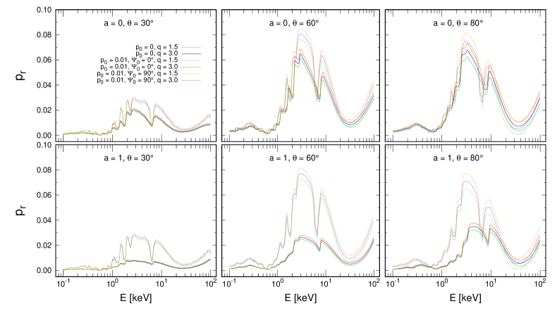
Figure A.19: The reflected-only polarisation degree, $p_{\mathrm{r}}$, versus energy for neutral disc (observed 2–10 flux $L_{\textrm{X}}/L_{\textrm{Edd}}\approx 10^{-5}$, see text for details), otherwise for the same parametric setup as in Figure A.18, displayed in the same manner.

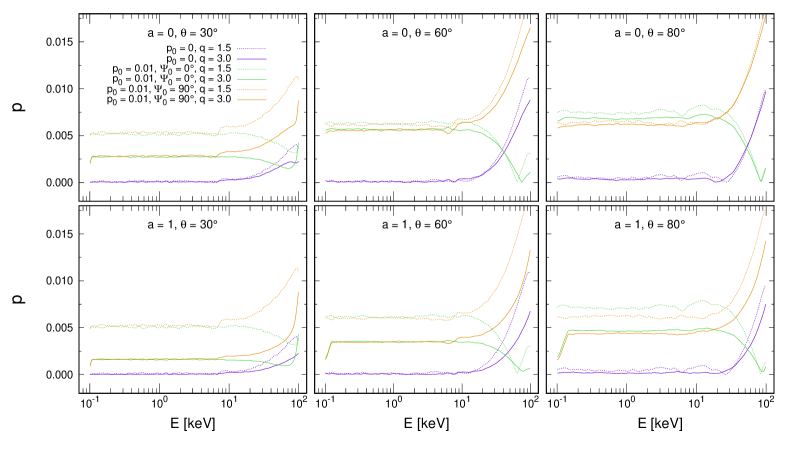
Figure A.20: The total polarisation degree, $p$, versus energy for the same parametric setup as in Figure A.18, displayed in the same manner.

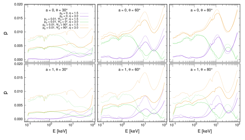
Figure A.21: The total polarisation degree, $p$, versus energy for the same parametric setup as in Figure A.19, displayed in the same manner.

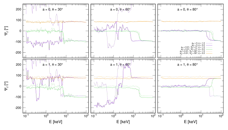
Figure A.22: The reflected-only polarisation angle, $\Psi_{\mathrm{r}}$, versus energy for the same parametric setup as in Figure A.18, displayed in the same manner.

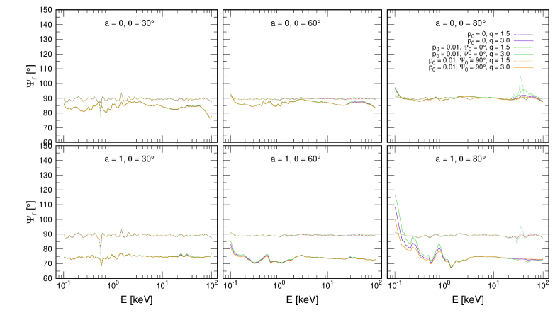
Figure A.23: The reflected-only polarisation angle, $\Psi_{\mathrm{r}}$, versus energy for neutral disc (observed 2–10 flux $L_{\textrm{X}}/L_{\textrm{Edd}}\approx 10^{-5}$, see text for details), otherwise for the same parametric setup as in Figure A.18, displayed in the same manner.

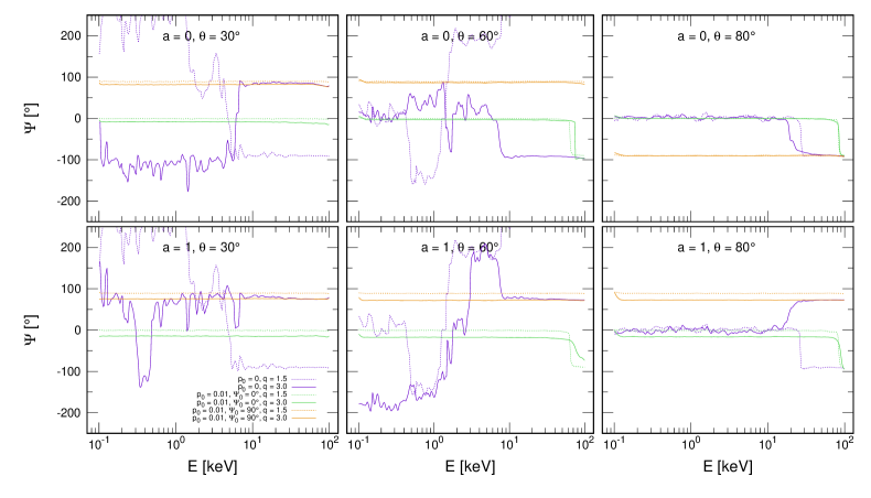
Figure A.24: The total polarisation angle, $\Psi$, versus energy for the same parametric setup as in Figure A.22, displayed in the same manner.

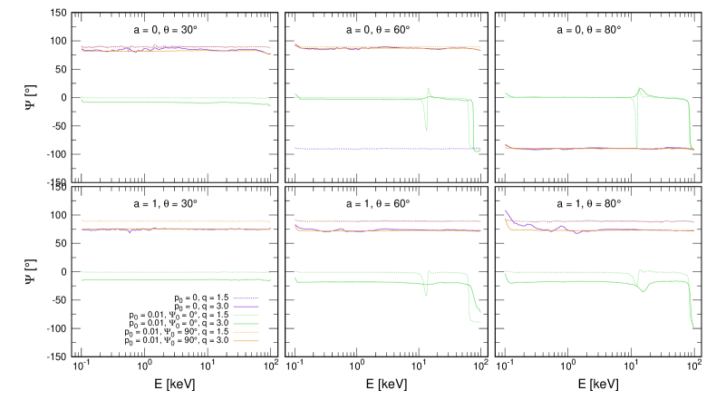
Figure A.25: The total polarisation angle, $\Psi$, versus energy for the same parametric setup as in Figure A.23, displayed in the same manner.

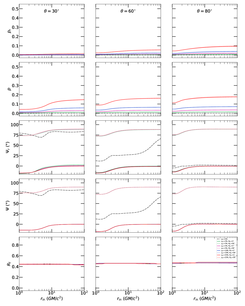
Figure A.26: The same as in Figure 3.11, but for the extended sandwich corona with $q=3$.

Supplementary figures to Chapter 4

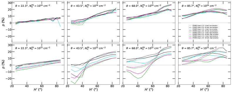
Figure A.27: The same as in Figure 4.5, but energy-averaged polarisation degree, $p$, versus half-opening angle $H^{\prime}$ is shown for $\theta=22.3\mbox{${}^{\circ}$}$, $\theta=43.5\mbox{${}^{\circ}$}$, $\theta=68.0\mbox{${}^{\circ}$}$, and $\theta=85.7\mbox{${}^{\circ}$}$ (left to right). Image adapted from Podgorný et al. [2023c].

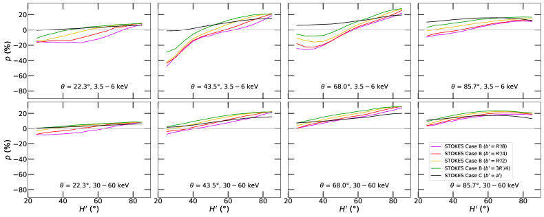
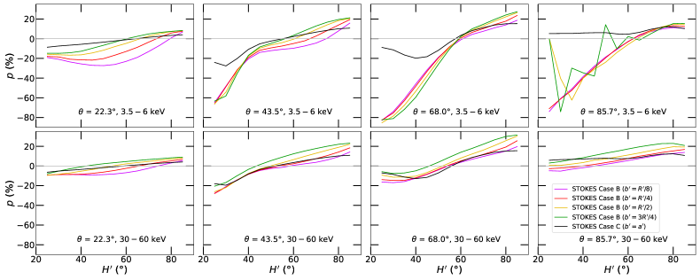
Figure A.28: The same as in Figure 4.6, but energy-averaged polarisation degree, $p$, versus half-opening angle $H^{\prime}$ is shown for $\theta=22.3\mbox{${}^{\circ}$}$, $\theta=43.5\mbox{${}^{\circ}$}$, $\theta=68.0\mbox{${}^{\circ}$}$, and $\theta=85.7\mbox{${}^{\circ}$}$ (left to right). Image adapted from Podgorný et al. [2023c].

Figure A.29: The same as in Figure A.28, but for $N_{\mathrm{H}}^{\textrm{eq}}=10^{25}\textrm{ cm}^{-2}$. Image adapted from Podgorný et al. [2023c].

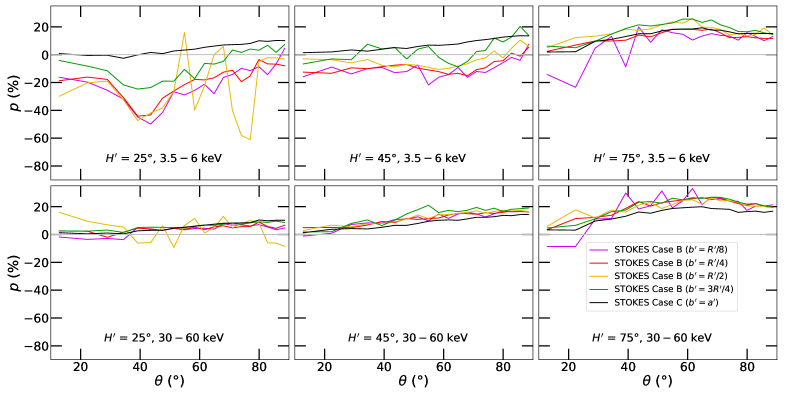
Figure A.30: The same as in Figure 4.6, but for low level of ionization, i.e. $\tau_{\textrm{e}}^{\textrm{eq}}=0.007$. Image adapted from Podgorný et al. [2023c].

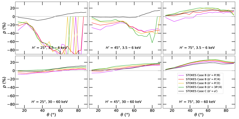
Figure A.31: The same as in Figure 4.7, but for low level of ionization, i.e. $\tau_{\textrm{e}}^{\textrm{eq}}=0.07$. Image adapted from Podgorný et al. [2023c].

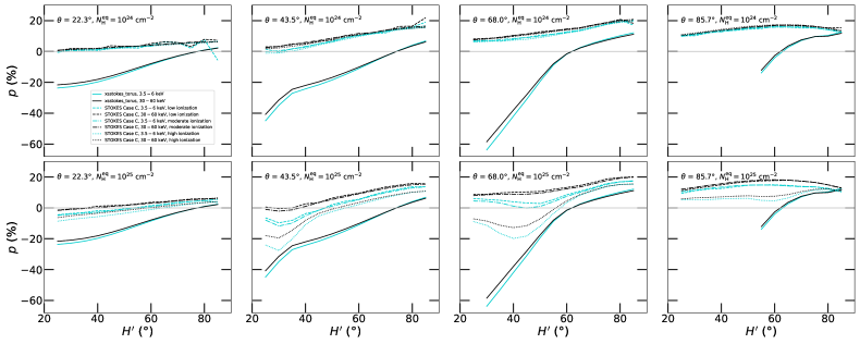
Figure A.32: The same as in Figure 4.11, but energy-averaged polarisation degree, $p$, versus half-opening angle $H^{\prime}$ is shown for $\theta=22.3\mbox{${}^{\circ}$}$, $\theta=43.5\mbox{${}^{\circ}$}$, $\theta=68.0\mbox{${}^{\circ}$}$, and $\theta=85.7\mbox{${}^{\circ}$}$ (left to right). Image adapted from Podgorný et al. [2023b].

Figure A.33: The incident radiation in the polar directions for AGNs modelled in Section 4.3: in the case of unpolarized coronal radiation (left) and $2\%$ parallelly polarized coronal radiation (middle) and $2\%$ perpendicularly polarized coronal radiation (right). We display from top to bottom the energy-dependent flux (in arbitrary units, corrected for the primary power-law slope) and the corresponding polarized flux, polarisation degree and polarisation angle. The computations from Marin et al. [2018a] are displayed in black and gray for $a=0$ and $a=1$, respectively. The new computations with KYNSTOKES for ionized disc are displayed in purple and pink for $a=0$ and $a=1$, respectively. Image adapted from Podgorný et al. [2024].

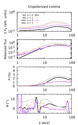
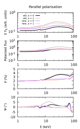
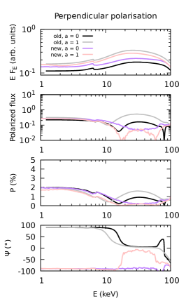
Figure A.34: The same as Figure A.33, but for neutral disc. Image adapted from Podgorný et al. [2024].

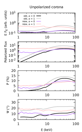
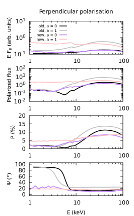
Figure A.35: The same as Figure A.33, but in the equatorial directions for AGNs modelled in Section 4.3. Image adapted from Podgorný et al. [2024].

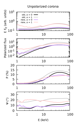
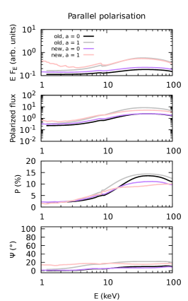
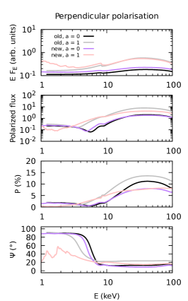
Figure A.36: The same as Figure A.35, but for neutral disc. Image adapted from Podgorný et al. [2024].

Supplementary figures to Chapter 5

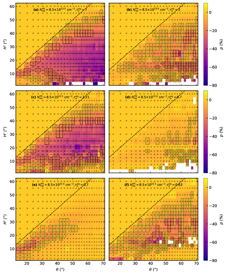
Figure A.37: The same as in Figure 5.3, but for a Case B elliptical obscurer with $b^{\prime}=R^{\prime}/8$. Image adapted from Podgorný et al. [2023c].

Figure A.38: The same as in Figure 5.3, but for a Case B elliptical obscurer with $b^{\prime}=3R^{\prime}/4$. Image adapted from Podgorný et al. [2023c].

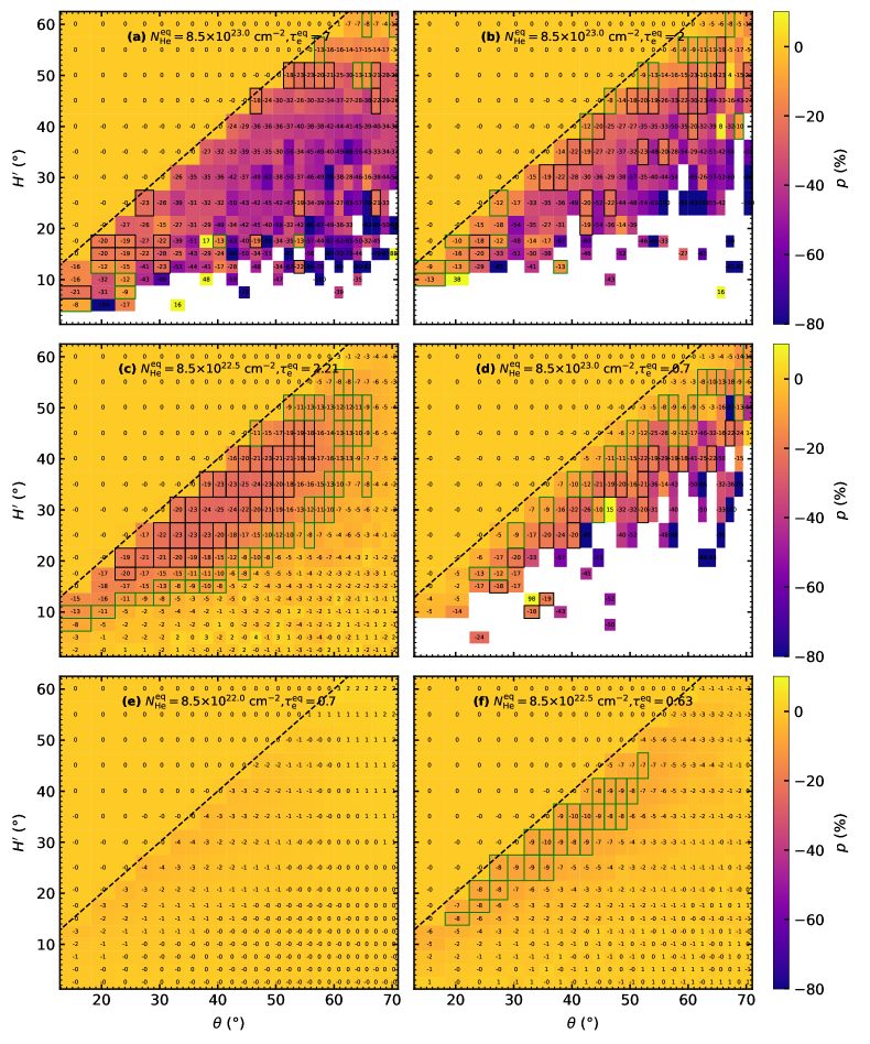
Figure A.39: The same as in Figure 5.3, but for a Case A wedge-shaped obscurer with $r_{\mathrm{out}}^{\textrm{torus}}=10$ and $r_{\textrm{in}}^{\textrm{torus}}=R^{\prime}-b^{\prime}$, where $b^{\prime}=a^{\prime}$ is consistently computed through (4.2) for any circular torus, depending on inclination $\theta$ and half-opening angle $H^{\prime}$. Image adapted from Podgorný et al. [2023c].

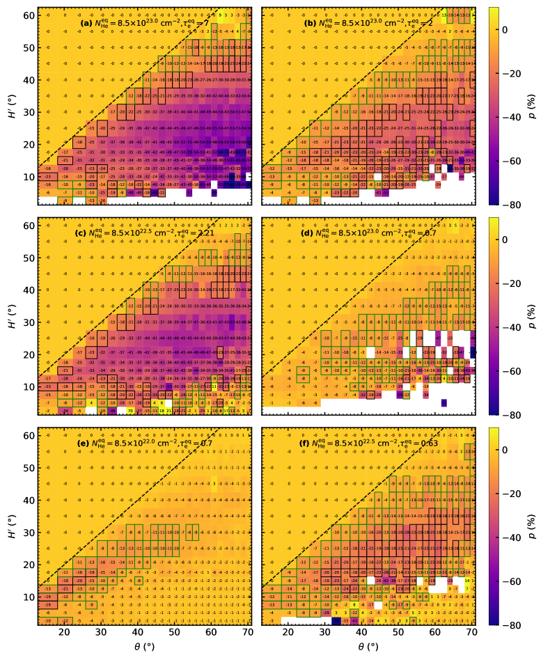
Figure A.40: The same as in Figure 5.3, but for $\Gamma=3$.

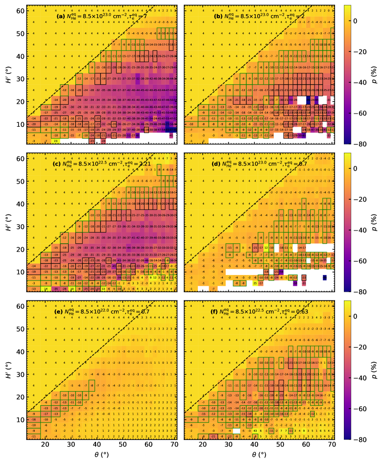
Figure A.41: The same as in Figure 5.3, but for $p_{0}=4\%$.

Figure A.42: The same as in Figure 5.3, but for $p_{0}=4\%$ and $\Gamma=3$.

Appendix B Singularities in general-relativistic surface integrals

The disc emission in equatorial plane can be two-dimensionally integrated in multiple ways: using the $\alpha$ and $\beta$ impact parameters, the related Carter’s constants of motion (see Appendix C), the Boyer-Lindquist coordinates $r$ and $\phi$, or using the $g$ factor instead of azimuthal $\phi$, and in forward or reversed integration order. Exact treatment of integrals of the kind (1.26) typically involves elliptical integrals of the first kind [Cunningham, 1975] and some simplifications, e.g. in radial emissivity profile, in directionality of the local emission, or in axial symmetry. On the contrary, numerical integration and tabular precomputation of geodesics, the transfer function, or other intermediate results, using discretization techniques, may lead to lack of precision and may not always be the most efficient option. In the latter approach, detailed computations of relativistic smearing of e.g. spectral lines tend to be in particular computationally expensive due to singularities in the integrand of various, but known kinds. Realizing quickly that an exploration and comparison of all possibilities would be of scope of another PhD thesis, we at least made an attempt of substituting the singularities in $g$ and $r$ coordinates with Gaussian quadratures [Gauss, 1814, Jacobi, 1826], as this is quickly possible, provided the expressions in Cunningham [1975] with singularity prescriptions. If the polynomial substitution proves to be significantly faster on a few examples, it may be worth of full implementation in the KY codes, where the current ide integrating subroutine works in the $r$ and $\phi$ coordinates and does not treat efficiently the singularities in $\phi$.

We will depart from Cunningham [1975], equation (7), which is basically (1.24) written with

$$g^{*}=\frac{g-g_{\textrm{min}}(r)}{g_{\textrm{max}}(r)-g_{\textrm{min}}(r)}\,,$$ (B.1)

which keeps $0\leq g^{*}\leq 1$. We will solve a few examples for undirectional Stokes parameter $I$ with the following emissivity profile

$$I\left(\frac{E_{\textrm{obs}}}{g},n_{\textrm{em}},r\right)=r^{-q}\bar{I}\left(\frac{E_{\textrm{obs}}}{g}\right)\,,$$ (B.2)

where $q=3$ is typically considered [Życki et al., 1998, Beckwith and Done, 2004, Dovčiak et al., 2014]. Then

$$N_{\textrm{E}} =\frac{\pi}{r_{0}^{2}}\int_{r_{\textrm{in}}}^{r_{\textrm{out}}}r^{1-q}\int_{0}^{1}\bar{I}\left(\frac{E_{\textrm{obs}}}{g^{*}[g_{\textrm{max}}-g_{\textrm{min}}]+g_{\textrm{min}}}\right)f(g^{*},r,\theta)$$ (B.3)

$$\,\,\,\,\,\,\,\,\,\,\,\,\,\,\,\,\,\,\,\,\,\,\,\,\,\,\,\,\,\,\,\,\,\,\,\,\,\,\,\,\,\,\,\,\,\,\cdot\frac{g^{*}[g_{\textrm{max}}-g_{\textrm{min}}]+g_{\textrm{min}}}{\sqrt{g^{*}}\sqrt{1-g^{*}}}\textrm{d}g^{*}\textrm{d}r$$

$$=\frac{\pi}{r_{0}^{2}}\int_{r_{\textrm{in}}}^{r_{\textrm{out}}}r^{1-q}\int_{-1}^{1}\bar{I}\left(\frac{E_{\textrm{obs}}}{\frac{1}{2}[\tilde{g}^{*}+1][g_{\textrm{max}}-g_{\textrm{min}}]+g_{\textrm{min}}}\right)$$

$$\,\,\,\,\,\,\,\,\,\,\,\,\,\,\,\,\,\,\,\,\,\,\,\,\,\,\,\,\,\,\,\,\,\,\,\,\,\,\,\,\,\,\,\,\,\,\cdot f\left(\frac{1}{2}[\tilde{g}^{*}+1],r,\theta\right)\Bigl{\{}\frac{1}{2}[\tilde{g}^{*}+1][g_{\textrm{max}}-g_{\textrm{min}}]+g_{\textrm{min}}\Bigr{\}}$$

$$\,\,\,\,\,\,\,\,\,\,\,\,\,\,\,\,\,\,\,\,\,\,\,\,\,\,\,\,\,\,\,\,\,\,\,\,\,\,\,\,\,\,\,\,\,\,\cdot\frac{1}{\sqrt{1-\tilde{g}^{*2}}}\textrm{d}\tilde{g}^{*}\textrm{d}r$$

$$=\frac{\pi}{r_{0}^{2}}\int_{r_{\textrm{in}}}^{r_{\textrm{out}}}r^{1-q}\int_{-1}^{1}\bar{F}(\tilde{g}^{*},r,\theta)\bar{S}(\tilde{g}^{*})\textrm{d}\tilde{g}^{*}\textrm{d}r\,\,,$$

where $\bar{S}(\tilde{g}^{*})=[1-\tilde{g}^{*2}]^{-\frac{1}{2}}$ is the diverging factor and $\bar{F}(\tilde{g}^{*},r,\theta)$ is an analytical function on $g^{*}\in[-1;1]$. This allows the usage of Chebyshev-Gauss quadrature formula [Ralston, 1965]

$$\int_{-1}^{1}\frac{1}{\sqrt{1-x^{2}}}\bar{F}(x)\textrm{d}x\approx\sum_{j=1}^{n}H_{j}\bar{F}(a_{j})\,,\,\,H_{j}=\frac{\pi}{n}\,,\,\,a_{j}=\cos\frac{[2j-1]\pi}{2n}\,.$$ (B.4)

We obtain

$$N_{\textrm{E}} =\frac{\pi^{2}}{nr_{0}^{2}}\int_{r_{\textrm{in}}}^{r_{\textrm{out}}}r^{1-q}\sum_{j=1}^{n}\bar{I}\left(\frac{E_{\textrm{obs}}}{\frac{1}{2}[\tilde{g}_{j}^{*}+1][g_{\textrm{max}}-g_{\textrm{min}}]+g_{\textrm{min}}}\right)$$ (B.5)

$$\,\,\,\,\,\,\,\,\,\,\,\,\,\,\,\,\,\,\,\,\,\,\,\,\,\,\,\,\,\,\,\cdot f\left(\frac{1}{2}[\tilde{g}_{j}^{*}+1],r,\theta\right)\Bigl{\{}\frac{1}{2}[\tilde{g}_{j}^{*}+1][g_{\textrm{max}}-g_{\textrm{min}}]+g_{\textrm{min}}\Bigr{\}}\textrm{d}r\,,$$

$$\,\,\,\,\,\,\,\,\,\,\,\,\,\,\,\,\,\,\,\,\,\,\,\,\,\,\,\,\,\,\,\,\,\tilde{g}_{j}=\cos\frac{[2j-1]\pi}{n}\,,$$

which can be compared to the more classical result in $g$ coordinate:

$$N_{\textrm{E}} =\frac{\pi}{r_{0}^{2}}\int_{r_{\textrm{in}}}^{r_{\textrm{out}}}r^{1-q}\int_{g_{\textrm{min}}}^{g_{\textrm{max}}}\bar{I}\left(\frac{E_{\textrm{obs}}}{g}\right)f\left(\frac{g-g_{\textrm{min}}}{g_{\textrm{max}}-g_{\textrm{min}}},r,\theta\right)$$ (B.6)

$$\,\,\,\,\,\,\,\,\,\,\,\,\,\,\,\,\,\,\,\,\,\,\,\,\,\,\,\,\,\,\,\cdot\frac{g}{\sqrt{g-g_{\textrm{min}}}\sqrt{g_{\textrm{max}}-g}}\textrm{d}g\textrm{d}r\,\,.$$

Figure B.1 provides examples of spectral line broadening for a distant observer for both, polynomial and classical integration in $g$ in the left and middle panels, respectively. Computational processing unit (CPU) time for a simple script on a laptop is provided, but only relative difference between the results of the two methods is important. A Gaussian line profile at $E_{\textrm{l}}=6.4$ keV was used

$$\bar{I}\left(\frac{E_{\textrm{obs}}}{g}\right)=\frac{1}{\omega\sqrt{2\pi}}e^{-\frac{\left[\frac{E_{\textrm{obs}}}{g}-E_{\textrm{l}}\right]^{2}}{2\omega^{2}}}\,,$$ (B.7)

where $g=\frac{1}{2}[\tilde{g}_{j}^{*}+1][g_{\textrm{max}}-g_{\textrm{min}}]+g_{\textrm{min}}$ for the case of (B.5). We used $\omega=0.005$ for the line width and 500 linearly spaced bins in energy between $E_{\textrm{min}}=1$ keV and $E_{\textrm{max}}=15$ keV. In the right panels, we provide referential results for intensity given by $\delta$ function, which automatically solves for the inner integral and is hence the fastest solution:

$$N_{\textrm{E}} =\frac{\pi}{E_{\textrm{obs}}r_{0}^{2}}\int_{r_{\textrm{in}}}^{r_{\textrm{out}}}r^{1-q}\int_{\frac{1}{g_{\textrm{min}}}}^{\frac{1}{g_{\textrm{max}}}}\delta\left(x^{\prime}-\frac{E_{\textrm{l}}}{E_{\textrm{obs}}}\right)f\left(\frac{\frac{1}{x^{\prime}}-g_{\textrm{min}}}{g_{\textrm{max}}-g_{\textrm{min}}},r,\theta\right)$$ (B.8)

$$\,\,\,\,\,\,\,\,\,\,\,\,\,\,\,\,\,\,\,\,\,\,\,\,\,\,\,\,\,\,\,\,\,\,\,\,\,\,\,\,\,\,\,\,\,\,\cdot\frac{1}{x^{\prime 2}\sqrt{1-g_{\textrm{min}}x^{\prime}}\sqrt{g_{\textrm{max}}x^{\prime}-1}}\textrm{d}x^{\prime}\textrm{d}r$$

$$=\begin{cases}\frac{E_{\textrm{obs}}\pi}{E_{\textrm{l}}^{2}r_{0}^{2}}\int_{r_{\textrm{in}}}^{r_{\textrm{out}}}r^{1-q}f\left(\frac{\frac{E_{\textrm{obs}}}{E_{\textrm{l}}}-g_{\textrm{min}}}{g_{\textrm{max}}-g_{\textrm{min}}},r,\theta\right)&\cdot\frac{1}{\sqrt{1-g_{\textrm{min}}\frac{E_{\textrm{l}}}{E_{\textrm{obs}}}}\sqrt{g_{\textrm{max}}\frac{E_{\textrm{l}}}{E_{\textrm{obs}}}-1}}\textrm{d}r\ ,\\ &\frac{E_{\textrm{l}}}{E_{0}}\in\left[\frac{1}{g_{\textrm{max}}};\frac{1}{g_{\textrm{min}}}\right]\ ,\\ 0\ ,&\textrm{else}\,\,,\end{cases}$$

where we used $x^{\prime}=1/g$. The results are provided for two linear binnings in $r$, given by $N_{\textrm{r}}$, and various binnings in $g$, given by $N_{\textrm{g}}$ (logarithmically compressed bins towards both integration edges starting from a mid-point), and various orders of $n$. For small $n$, we first observe $n$ nodes in the numerical defocusing, which gets smoothed to the exact result when $n$ approaches infinity. The unnatural features from realistic line profiles are given by the fact that we in addition imposed an approximation of the transfer function $\bar{f}_{\textrm{T}}$ [see Cunningham, 1975] given by empirical law representing the curve $\bar{f}_{\textrm{T}}(r)$ from figure 3a of Cunningham [1975] and the same for $g_{\textrm{min}}(r)$ and $g_{\textrm{max}}(r)$ from figure 1a of Cunningham [1975], all for $a=0$ and $\cos\theta=0.75$, as if these were constants in $\theta$. The remaining parameters were $q=3$, $r_{\textrm{in}}=2\,r_{\textrm{g}}$, $r_{\textrm{out}}=100\,r_{\textrm{g}}$. The integrations in $r$ and $g$ were performed using the Simpson rule [see e.g. Ralston, 1965].

Figure B.1: Comparison of a narrow Gaussian line that is relativistically smeared for a distant observer, using the proposed polynomial integration technique (left) and using the classical integration in $g$ (middle) for various precision. Each case is renormalized to arbitrary value for viewing clarity. The reference image of a smeared line profile given by $\delta$ function is also shown (right). The results are displayed for $N_{\textrm{r}}=500$ (top) and $N_{\textrm{r}}=10000$ (bottom). The results are approximate, given significant simplifications (see text), as the main purpose is to test a few examples of different integration methods.

Although some gain in efficiency is apparent, the polynomial approach did not seem to win dramatically over the integration in classical $g$ and $r$ coordinates, when also more detailed examples were tested than the above shown. We tried for interpolation of tabular emissivity profiles in discrete energy bins and precomputed transfer functions from Dovčiak [2004]. We tried the usage of quadratures in $g$-integration compared to splitting the classical inner integral in (B.6) in three parts: the edges with singularities to be analytically integrated for quadratic interpolation of the non-diverging part of the integrand, and the mid part to be numerically integrated, using the Simpson rule. Various binning types, resolutions and line profiles were also tested. The intermediate results are disfavoring continuation of this work, but perhaps a negative result of an experiment also deserves to be recorded.

Appendix C General-relativistic change of the polarisation angle

We will summarize the derivations of the change of the polarisation angle due to GR effects in Kerr spacetime in between the lamp-post and the observer and in between the lamp-post and the disc. The original calculations were carried by Michal Dovčiak and in the scope of this dissertation only revisited and verified. These are now implemented in the KYNSTOKES code [Podgorný et al., 2023a].

It is practical to use two Carter’s constants of motion that are related to the impact parameters $\alpha$ and $\beta$. These will have a reduced form $\bar{\lambda}=\alpha\sin{\theta}=0$, $\bar{q}=\sqrt{\beta^{2}+(\alpha^{2}-a^{2})\cos^{2}{\!\theta}}=\sqrt{\beta^{2}-a^{2}\cos^{2}{\!\theta}}$, because we track only the photons from the rotation axis. The expressions for $p_{\mu}$ components are taken from Carter [1968], Misner et al. [1973]: $|p_{\theta}|=\sqrt{\bar{q}^{2}+a^{2}\cos^{2}\!\theta}$, $|p_{r}|=\sqrt{(r^{2}+a^{2})^{2}-\Delta(\bar{q}^{2}+a^{2})}/\Delta$ with $\Delta=r^{2}-2r+a^{2}$; $p_{\phi}=0$ is trivial and we normalize the conserved energy as $p_{t}=-1$. We define the unit polarisation 3-vector $\vec{f}$ in the polarisation plane (perpendicular to the photon’s momentum) and a disc normal (or rotation axis) projected to that plane, which altogether set the polarisation angle $\Psi$ in any local frame of reference. We will first draft the general procedure and then solve for particular expressions of $\Delta\Psi$ between the lamp and the observer, denoted as $\chi_{\textrm{p}}$, and between the lamp and the disc, denoted as $\chi_{\textrm{d}}$.

We assume the initial polarisation angle $\Psi_{0}=0$ at the lamp location. For incident polarisation at the lamp in the local reference frame of the primary source (defined by the height, $h$, and constant of motion, $\bar{q}$) we write $\vec{f_{0}}$. This local frame is given by an orthonormal tetrade $e_{\rm(a)}^{\mu}$, which sets four components of a polarisation 4-vector $f_{0}^{\rm(a)}=(0,\vec{f_{0}})$, the corresponding polarisation 4-vector being $f_{0}^{\mu}=e_{\!\rm(a)}^{\mu}f_{0}^{\rm(a)}$. This 4-vector can be parallelly transported in Kerr spacetime, using (1.22), between the lamp and a distant observer at spatial infinity (defined by the observer inclination, $\theta$), or between the lamp and the disc (defined by the radius, $r$). At each receiving point, the polarisation 4-vector $f^{\mu}$ will, generally, have a non-zero time component in the local reference frame. We will thus subtract a multiple of a null vector after the parallel transport, so that the properties of a polarisation vector are kept, i.e. the time component is set to zero and the space part is not rotated. This means transforming

$$f^{\prime\textrm{(a)}}=f^{\textrm{(a)}}-\frac{f^{\textrm{(t)}}}{p^{\textrm{(t)}}}p^{\textrm{(a)}}\,.$$ (C.1)

Using the Walker-Penrose theorem and (1.27), we will express $\kappa_{1}$ and $\kappa_{2}$ by means of the initial $p^{\mu}$ and $f_{0}^{\mu}$ of each photon and the same for the three unknown components of the polarisation 4-vector $f^{\mu}$ in a given local reference frame at the receiving point, where we will construct the $\Psi$ with respect to the projected disc normal (or rotation axis).

Let us first solve the case of transfer from the lamp to a distant observer. At the lamp it holds that

$$\kappa_{1}=h\sqrt{\frac{\bar{q}^{2}+a^{2}}{h^{2}+a^{2}}}\,,$$ (C.2)

$$\kappa_{2}=-a\sqrt{\frac{\bar{q}^{2}+a^{2}}{h^{2}+a^{2}}}\,,$$ (C.3)

where we set $f_{0\,t}=f_{0\,\phi}=0$ and the other two components, $f_{0\,r}$ and $f_{0\,\theta}$ are obtained from general conditions of (i) polarisation vector being perpendicular to the momentum, $f^{\mu}p_{\mu}=0$, and (ii) polarisation vector being normalized to unity, $f_{\mu}f^{\mu}=1$. Using the conditions $f^{\mu}p_{\mu}=p^{\mu}p_{\mu}=0$, we perform the transformation (C.1) at spatial infinity

$$f^{\prime\textrm{(t)}}=0\,,$$ (C.4)

$$f^{\prime\textrm{(r)}}=r^{2}p^{\theta}(p^{\theta}f^{r}-p^{r}f^{\theta})\,,$$ (C.5)

$$f^{\prime(\theta)}=rp^{r}(p^{\theta}f^{r}-p^{r}f^{\theta})\,,$$ (C.6)

$$f^{\prime(\phi)}=r\sin{\theta}f^{\phi}\,,$$ (C.7)

where $f^{\mu}$ and $p^{\mu}$ were transformed into the local reference frame defined by the orthonormal tetrade $e^{\textrm{(t)}}_{\mu}=(-1,0,0,0)$, $e^{\textrm{(r)}}_{\mu}=(0,1,0,0)$, $e^{(\theta)}_{\mu}=-r\,(0,0,1,0)$, $e^{(\phi)}_{\mu}=r\sin{\theta}\,(0,0,0,1)$. Combining (C.4)–(C.7) with (1.27) gives $\kappa_{1}$ and $\kappa_{2}$ for each geodesic at spatial infinity

$$\kappa_{1}=\beta f^{\prime(\theta)}+a\sin{\theta}f^{\prime(\phi)}\,,$$ (C.8)

$$\kappa_{2}=-a\sin{\theta}f^{\prime(\theta)}+\beta f^{\prime(\phi)}\,.$$ (C.9)

In the end we put (C.8) equal to (C.2) and (C.9) equal to (C.3), which brings the expression for the change of the polarisation angle $\chi_{\rm p}$ at the local reference frame of the observer

$$\tan{\chi_{\rm p}}=-\frac{f^{\prime(\phi)}}{f^{\prime(\theta)}}=a\frac{\beta-h\sin{\theta}}{a^{2}\sin{\theta}+h\beta}\,.$$ (C.10)

The dependence of $\chi_{\rm p}(h)$ on height is shown in Figure C.2 for maximally rotating black hole and three observer inclinations.

Figure C.1: The GR change of polarisation angle, $\chi_{\rm p}$, between the lamp-post and the observer versus lamp-post height $h$ for black-hole spin $a=1$ and three different observer’s inclinations $\theta=30^{\circ},\,60^{\circ}$, and $85^{\circ}$. Image courtesy of Michal Dovčiak.

Figure C.2: The GR change of the polarisation angle, $\chi_{\rm d}$, between the lamp-post and the disc as a function of radius $r$ in the equatorial plane for black-hole spin $a=1$ and several lamp-post heights. Image courtesy of Michal Dovčiak.

Now we will solve for the change of polarisation angle between the lamp and the disc. In the equatorial plane, (1.27) yields

$$\kappa_{1}=\frac{r^{2}+a^{2}}{r}p_{r}f_{t}+\frac{r^{2}+a^{2}}{r}f_{r}+\frac{ap_{r}}{r}f_{\phi}\,,$$ (C.11)

$$\kappa_{2}=\frac{ap_{\theta}}{r}f_{t}+\frac{a}{r}f_{\theta}+\frac{p_{\theta}}{r}f_{\phi}\,.$$ (C.12)

A notable simplification of the computations comes from expressing $f_{t}$, $f_{\theta}$, $f_{\phi}$ as functions of $\kappa_{1}$, $\kappa_{2}$, $p^{\theta}$, $p^{r}$ and the metric coefficients, using the conditions $p_{\mu}p^{\mu}=0$, $f^{\mu}p_{\mu}=0$ and $f_{\mu}f^{\mu}=1$. Instead of performing transformation in the form of (C.1), we will subtract the $r$-component of $f_{\mu}$ in the equatorial plane

$$f^{\prime}_{\mu}=f_{\mu}-\frac{f_{r}}{p_{r}}p_{\mu}\,,$$ (C.13)

because this also largely simplifies expressions. Since the polarisation vector is orthogonal to the photon momentum and definition of the polarisation angle is in the plane orthogonal to the photon momentum, any transformation $f^{\prime}_{\mu}=f_{\mu}+Ap_{\mu}$ does not change its value (the tetrade vectors $e_{\rm(y)}^{\mu}$ and $e_{\rm(z)}^{\mu}$, defined below, into which we project the polarisation vector $f^{\prime\mu}$ in the polarisation angle definition at the disc, are perpendicular to the photon momentum). Hence, we obtain the reduced components of $f^{\prime}_{\mu}$ in the form of

$$f^{\prime}_{t}=-\frac{\Delta p^{\theta}}{ar(p^{r})^{2}}\kappa_{2}+\left[\frac{(r^{2}+a^{2})}{a}\frac{\Delta(p^{\theta})^{2}}{(p^{r})^{2}}+g_{t\phi}\right]\frac{f_{\phi}}{g_{\phi\phi}}\,,$$ (C.14)

$$f^{\prime}_{r}=0\,,$$ (C.15)

$$f^{\prime}_{\theta}=\frac{g_{\phi\phi}}{ar(p^{r})^{2}}\kappa_{2}-\frac{(r^{2}+a^{2})p^{\theta}}{a(p^{r})^{2}}f_{\phi}\,,$$ (C.16)

$$f^{\prime}_{\phi}=f_{\phi}=\frac{arp^{r}\kappa_{1}+r(r^{2}+a^{2})p^{\theta}\kappa_{2}}{q^{2}+a^{2}}\,,$$ (C.17)

where $g_{t\phi}=-2a/r$, $g_{\phi\phi}=[(r^{2}+a^{2})^{2}-\Delta a^{2}]/r^{2}$ are taken from the Kerr metric in the equatorial plane. The components of the 4-velocity are $U^{t}=(r^{2}+a\sqrt{r})/r/\sqrt{r^{2}-3r+2a\sqrt{r}}$, $U^{r}=U^{\theta}=0$ and $U^{\phi}=\Omega_{\rm K}U^{t}$ with relativistic Keplerian rotational velocity $\Omega_{\rm K}=(r^{3/2}+a)^{-1}$ [Novikov and Thorne, 1973]. We construct an orthonormal tetrade in the local comoving frame with the disc, in order to define the polarisation angle $\chi_{\textrm{d}}$. We choose the time-like tetrade vector to be given by the 4-velocity of the orbiting material, the first spatial tetrade vector to be directed in the direction of momentum of the incoming photon, the second spatial tetrade vector to be defined by the projection of the local disc normal into the plane orthogonal to the photon momentum, and the last spatial tetrade vector is constructed as the vector product of the others, so that the full orthonormal tetrade is formed. Thus, we set

$$e_{\rm(t)}^{\mu}=U^{\mu}\,,$$ (C.18)

$$e_{\rm(x)}^{\mu}=\frac{p^{\mu}+p^{\nu}U_{\nu}U^{\mu}}{-p_{\sigma}U^{\sigma}}\,,$$ (C.19)

$$e_{\rm(y)}^{\mu}=\frac{n^{\mu}-\frac{n_{\nu}p^{\nu}}{-p_{\sigma}U^{\sigma}}e_{\rm(x)}^{\mu}}{\sqrt{1-\left(\frac{n_{\rho}p^{\rho}}{p_{\iota}U^{\iota}}\right)^{2}}}\,,$$ (C.20)

$$e_{\rm(z)}^{\mu}=\frac{\varepsilon^{\alpha\beta\gamma\mu}U_{\alpha}p_{\beta}n_{\gamma}}{-p_{\sigma}U^{\sigma}\sqrt{1-\left(\frac{n_{\rho}p^{\rho}}{p_{\iota}U^{\iota}}\right)^{2}}}\,,$$ (C.21)

where $\varepsilon^{\alpha\beta\gamma\mu}=-\delta^{\alpha\beta\gamma\mu}/\sqrt{-\hat{g}}$ is the permutation tensor defined by the permutation symbol, $\delta^{\alpha\beta\gamma\mu}$, and the metric tensor determinant, $\sqrt{-\hat{g}}=r^{2}$, and $n^{\mu}=(0,0,-1/r,0)$ is the local disc’s normal. Using the relations $f^{\mu}p_{\mu}=0$, $U_{\theta}=0$, $p_{\phi}=0$, (C.15), (C.18)–(C.21) we obtain the expression for the change of polarisation angle $\chi_{\textrm{d}}$ at the local reference frame of the observer comoving with the disc

$$\tan{\chi_{\textrm{d}}}=\frac{e_{\rm(z)}^{\mu}f^{\prime}_{\mu}}{e_{\rm(y)}^{\mu}f^{\prime}_{\mu}}=\frac{U_{t}p_{r}f^{\prime}_{\phi}+U_{r}f^{\prime}_{\phi}-U_{\phi}p_{r}f^{\prime}_{t}}{p_{\nu}U^{\nu}f^{\prime}_{\theta}-qU^{\mu}f^{\prime}_{\mu}}\,,$$ (C.22)

where $U^{\mu}f^{\prime}_{\mu}=U^{t}f^{\prime}_{t}+U^{\phi}f^{\prime}_{\phi}$, $p_{\nu}U^{\nu}=-U^{t}$, $f^{\prime}_{t}$, $f^{\prime}_{\theta}$ and $f^{\prime}_{\phi}$ follow from (C.14), (C.16) and (C.17), respectively, where the constants $\kappa_{1}$ and $\kappa_{2}$ have to be taken from (C.2) and (C.3), respectively. The dependence of $\chi_{\rm d}(r)$ is shown in Figure C.2 for maximally rotating black hole and several lamp-post heights.

Appendix D Axially symmetric reflection models for XSPEC

Both variants of the xsstokes C routine that are presented in Section 4.2 operate on the same basis. We produce the Stokes parameters $I$, $Q$ and $U$ in particular reflection geometry for three independent primary polarisation states with unpolarized and $100\%$ horizontally ($\Psi_{0}=\frac{\pi}{2}$) and $100\%$ diagonally ($\Psi_{0}=\frac{\pi}{4}$) polarized irradiation, in order to use equation (4.3). These tables were first produced in the American Standard Code for Information Interchange (ASCII) text file format and then converted to FITS tables in the OGIP format, using XSPEC Table Model Generator. This simple conversion script in Python 3 was developed by Michal Bursa, but also verified with a similar routine independently developed in the scope of this dissertation. We stress the usefulness of the XSPEC Table Model Generator for obtaining any tabular models for XSPEC version 12.13.0 (and onwards) suitable for polarisation. A reduction of the code to a pure spectral FITS file generation (necessary for previous XSPEC versions) is straight forward within. The xsstokes code can be adapted to any precomputed non-relativistic static model of axially symmetric reflector, where the formula (4.3) would apply and where the three tabular dependencies could be converted to the right format using the XSPEC Table Model Generator.

In Section 4.2, we already explained how we obtained the tabular dependencies for xsstokes_disc. For xsstokes_torus the precomputations were only a bit more demanding, requiring development of a Python 3 routine, called torus_integrator. We provide here the details of the numerical implementation not only for the sake of reproducibility of the results presented in Section 4.2.1, but because we also believe that the routine may be useful for other purposes. The mechanisms of integration of precomputed spectropolarimetric reflection tables over the two-dimensional surface are wavelength independent and can be easily adapted to elliptical tori, for example. Different local reflection tables for different irradiation can be used, aiming at higher accuracy for the description of AGN tori, or reflecting media of completely different astrophysical origin.

Inside the torus_integrator routine, the user can define an isotropically emitting power-law point source located at the center of the coordinates (see Figure 4.10) with $1.2\leq\Gamma\leq 3.0$ and a state of incident polarisation, given by the primary polarisation degree $p_{0}$ and primary polarisation angle $\Psi_{0}$. These parameters should preserve the values given by the local reflection tables, as the interpolation is not performed for these parameters for efficiency reasons. Then the user selects any torus half-opening angle $1\mbox{${}^{\circ}$}<H^{\prime}<90\mbox{${}^{\circ}$}$ and any observer’s inclination $0\mbox{${}^{\circ}$}<\theta<90\mbox{${}^{\circ}$}$, both measured from the pole. In the current setup, the results are independent of the distance of the torus from the center $r_{\textrm{in}}^{\textrm{torus}}$ (see below). The user also selects integration resolution in the coordinates $u\in(0,2\pi]$ and $v\in[\pi-H^{\prime},\pi]$, where the grid is linearly divided in $N_{\textrm{v}}$ and $2N_{\textrm{u}}$ bins in the corresponding ranges (the number of bins in $u$ covers only the $[\frac{\pi}{2},\frac{3\pi}{2}]$ interval, because the other half is symmetrically added). The energy binning of the output is preserved from the local reflection tables and the output is stored in ASCII file format with lower and upper energy bin edges and the corresponding renormalized Stokes parameters $I$, $Q$ and $U$. If a list of model parameter values is given, multiple files will be stored in the output directory under names of all parameters and their values.

We utilize standard relations between the cartesian coordinate system {$x$, $y$, $z$} given by the base vectors $\vec{e}_{\textrm{x}}=(1,0,0)$, $\vec{e}_{\textrm{y}}=(0,1,0)$, $\vec{e}_{\textrm{z}}=(0,0,1)$ and the torus surface coordinates {$u$, $v$} given by the base vectors $\frac{\partial}{\partial u}=(-\sin{u},\cos{u},0)$, $\frac{\partial}{\partial v}=(-\sin{v}\cos{u},-\sin{v}\sin{u},\cos{v})$ (see Figure 4.10):

$$x =(R^{\prime}+r^{\prime}\cos{v})\cos{u}\textrm{ ,}$$ (D.1)

$$y =(R^{\prime}+r^{\prime}\cos{v})\sin{u}\textrm{ ,}$$

$$z =r^{\prime}\sin{v}\textrm{ ,}$$

where $R^{\prime}=r^{\prime}+r_{\textrm{in}}^{\textrm{torus}}$ is the distance between (0,0,0) and the center of the meridional section of the torus, and

$$r^{\prime}=r_{\textrm{in}}^{\textrm{torus}}\frac{\cos{H^{\prime}}}{1-\cos{H^{\prime}}}$$ (D.2)

is the radius of the toroidal section circles in the meridional plane, following equation (4.2). The surface is given by another well-known implicit formula

$$\Phi=(x^{2}+y^{2}+z^{2}+R^{\prime 2}-r^{\prime 2})^{2}-4R^{\prime 2}(x^{2}+y^{2})=0\textrm{ .}$$ (D.3)

The local reflection tables from Podgorný et al. [2022] are linearly interpolated at each at each point in the {$u$, $v$} grid in $\mu_{\textrm{i}}=\cos{\delta_{\textrm{i}}}$, $\mu_{\textrm{e}}=\cos{\delta_{\textrm{e}}}$, and $\Phi_{\textrm{e}}$, which are schematically shown in Figure D.1 (left). We first precompute all three angles at each grid point in the local frame, given by the local surface normal $\vec{n}=\frac{\nabla\Phi}{\lvert\nabla\Phi\rvert}$, the incident vector $\vec{I}=(x,y,z)$, the emission vector $\vec{K}=(0,\sin\theta,\cos\theta)$, and their respective projections $\vec{I}_{\textrm{p}}$ and $\vec{K}_{\textrm{p}}$ to the local tangent plane through scalar products.

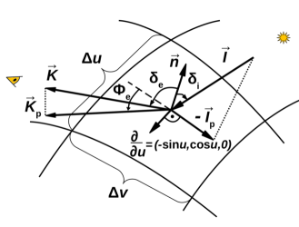
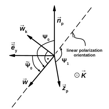
Figure D.1: Left: the definitions of angles and vectors in the locally reflecting plane, tangent to the torus surface. Right: the definitions of angles and vectors in the polarisation plane, perprendicular to the photon momentum direction. These are needed for the calculations of rotation of the polarisation angle by changing frame of reference. Image adapted from Podgorný et al. [2023b].

The code secures that the grid points with $\delta_{\textrm{i}}\notin[0,\frac{\pi}{2}]$ and $\delta_{\textrm{e}}\notin[0,\frac{\pi}{2}]$ are not accounted for. We limit $\pi-H^{\prime}\leq v\leq\pi$, i.e. we do not account for those regions that lie below the equatorial plane and for any $v$ smaller than the shadow boundary constrained by $H^{\prime}$. The region of reflection has to be also directly visible by the observer, which is for each $u$ and $\theta$ given by the boundary curve of the zero-transparency condition $0=\vec{n}\cdot\vec{K}$. Therefore, after a few simple steps we arrive at a prescription for this curve

$$v_{\textrm{limit}}(u,\theta)=-\arctan(2\sin u\tan\theta)+\pi\textrm{ .}$$ (D.4)

Next, we have to account for self-obscuration of the reflected rays by the opposite side of the torus, closer to the observer. This is the scenario for highly inclined observers. To select such region, we define a grazing vector $\vec{G}$ that begins at $\vec{X}_{1}=$ ($x_{1}$, $y_{1}$, $z_{1}$) at the opposite half-space from the observer given by $\pi\leq u\leq 2\pi$ and some $v_{\textrm{self-obs}}$ per each $u$. The grazing vector $\vec{G}$ points in the $\vec{K}$ direction towards the observer and ends at a point $\vec{X}_{2}=$ ($x_{2}$, $y_{2}$, $z_{2}$) tangential to the torus surface, i.e. defined by $v_{\textrm{limit}}$ for unknown $0\leq u_{\textrm{t}}\leq\pi$. Thus, parametrically for $\vec{X}_{1}+t\vec{K}=\vec{X}_{2}$ we write

$$(R^{\prime}+r^{\prime}\cos v_{\textrm{self-obs}})\cos u+tK_{1} =(R^{\prime}+r^{\prime}\cos v_{\textrm{limit}})\cos u_{\textrm{t}}\textrm{ ,}$$ (D.5)

$$(R^{\prime}+r^{\prime}\cos v_{\textrm{self-obs}})\sin u+tK_{2} =(R^{\prime}+r^{\prime}\cos v_{\textrm{limit}})\sin u_{\textrm{t}}\textrm{ ,}$$

$$r^{\prime}\sin v_{\textrm{self-obs}}+tK_{3} =r^{\prime}\sin v_{\textrm{limit}}\textrm{ .}$$

Then, the limiting curve $v_{\textrm{self-obs}}(u,\theta)$ is found as a solution {$v_{\textrm{self-obs}},t,u_{\textrm{t}}$} of a set of equations

$$0 =(R^{\prime}+r^{\prime}\cos v_{\textrm{self-obs}})\cos u-(R^{\prime}+r^{\prime}\cos v_{\textrm{limit}}(u_{\textrm{t}},\theta))\cos u_{\textrm{t}}\textrm{ ,}$$ (D.6)

$$0 =(R^{\prime}+r^{\prime}\cos v_{\textrm{self-obs}})\sin u+t\sin\theta-(R^{\prime}+r^{\prime}\cos v_{\textrm{limit}}(u_{\textrm{t}},\theta))\sin u_{\textrm{t}}\textrm{ ,}$$

$$0 =r^{\prime}\sin v_{\textrm{self-obs}}+t\cos\theta-r^{\prime}\sin v_{\textrm{limit}}(u_{\textrm{t}},\theta)\textrm{ .}$$

Each local scattering surface in the user-defined grid is given by boundaries $v_{1}(u,v)$, $v_{2}(u,v)$, $u_{1}(u,v)$, $u_{2}(u,v)$. Or the local surface is set to zero, if the central bin point {$u$, $v$} does not fall within the restricting boundary conditions above, which is valid for sufficiently high resolution. We then approximate the contributing local scattering surfaces by a tangent rectangle with area

$$\begin{split}A_{\textrm{u,v}}&=\int_{u_{1}}^{u_{2}}\int_{v_{1}}^{v_{2}}r^{\prime}(R^{\prime}+r^{\prime}\cos v)dvdu\\ &\approx r^{\prime}(R^{\prime}+r^{\prime}\cos v)(v_{2}-v_{1})(u_{2}-u_{1})\textrm{ .}\end{split}$$ (D.7)

At each {$u,v$} we perform the tri-linear interpolation in the local reflection angles $\mu_{\textrm{i}}$, $\mu_{\textrm{e}}$, and $\Phi_{\textrm{e}}$ of the tabulated Stokes parameters $I$, $Q$ and $U$, commonly denoted as $S(\mu_{\textrm{i}},\mu_{\textrm{e}},\Phi_{\textrm{e}};E,\Gamma,p_{0},\Psi_{0})$. The interpolated result, which we denote as $\bar{S}_{\textrm{u,v}}(\mu_{\textrm{i}}(u,v),\mu_{\textrm{e}}(u,v),\Phi_{\textrm{e}}(u,v);E,\Gamma,p_{0},\Psi_{0})$, is further transformed.

The polarisation vector of the interpolated reflected rays needs to be rotated from the local frame to conform to the photon momentum direction in the global system. In global coordinates, the Stokes parameters are defined with respect to the system axis of symmetry. The incident electric vector orientation does not have to be rotated to conform to the polarisation definition in the local frame due to the axial symmetry of the reflecting surface and due to the placement of the point-source in the central point. The polarisation fraction after the rotation $p_{1}$ is equal to the $p_{0}$ in the local reflection frame. Similarly for the intensity, $I_{1}=I_{0}$. Hence, for the remaining Stokes parameters we have $Q_{1}=\sqrt{Q_{0}^{2}+U_{0}^{2}}\cos{(2\Psi_{1})}$ and $U_{1}=\sqrt{Q_{0}^{2}+U_{0}^{2}}\sin{(2\Psi_{1})}$. In order to obtain the $\Psi_{1}(\Psi_{0})$ function, we will go back to the adopted definitions (1.10), which are illustrated in Figure D.1 (right) in the polarisation plane. We assume $\Psi_{0}$ with respect to the projected normal $\vec{n}_{\textrm{p}}=\vec{n}-(\vec{n}\cdot\vec{K})\vec{K}$ and $\Psi_{1}$ with respect to the projected global axis of symmetry $\vec{z}_{\textrm{p}}=\vec{e}_{\textrm{z}}-(\vec{e}_{\textrm{z}}\cdot\vec{K})\vec{K}$. Then $\vec{\tilde{e}}_{\textrm{y}}=\vec{K}\times\frac{\vec{n}_{\textrm{p}}}{\lvert\vec{n}_{\textrm{p}}\rvert}$, $\vec{\tilde{e}}_{\textrm{x}}=\frac{\vec{n}_{\textrm{p}}}{\lvert\vec{n}_{\textrm{p}}\rvert}$ and $\vec{\tilde{e}}_{\textrm{z}}=\vec{K}$ are the base vectors in the polarisation plane and the polarisation vector is locally $\vec{w}_{\textrm{loc}}=(\cos{\Psi_{0}},\sin{\Psi_{0}},0)$. The conditions $\cos{\Psi_{0}}=\vec{\tilde{e}}_{\textrm{x}}\cdot\vec{w}$, $\cos{\tilde{\Psi}_{0}}=\sin{\Psi_{0}}=\vec{\tilde{e}}_{\textrm{y}}\cdot\vec{w}$ and $\vec{w}\cdot\vec{K}=0$ provide

$$\vec{w}_{\textrm{loc}}=\begin{pmatrix}\vec{\tilde{e}}_{\textrm{x}},&\vec{\tilde{e}}_{\textrm{y}},&\vec{\tilde{e}}_{\textrm{z}}\end{pmatrix}\cdot\vec{w}=B\cdot\vec{w}\textrm{ .}$$ (D.8)

Therefore, we solve for this matrix equation to get $\vec{w}=B^{-1}\cdot\vec{w}_{\textrm{loc}}$, in order to obtain $\vec{w}_{\textrm{k}}=-\vec{K}\times\vec{w}$. In the end,

$$\Psi_{1}=\begin{cases}\arccos{\left(\dfrac{\vec{z}_{\textrm{p}}\cdot\vec{w}}{\lvert\vec{z}_{\textrm{p}}\rvert\lvert\vec{w}\rvert}\right)}\ ,&\textrm{if}\ \arccos{\left(\dfrac{\vec{z}_{\textrm{p}}\cdot\vec{w}_{\textrm{k}}}{\lvert\vec{z}_{\textrm{p}}\rvert\lvert\vec{w}_{\textrm{k}}\rvert}\right)}\leq\dfrac{\pi}{2}\textrm{ ,}\\ -\arccos{\left(\dfrac{\vec{z}_{\textrm{p}}\cdot\vec{w}}{\lvert\vec{z}_{\textrm{p}}\rvert\lvert\vec{w}\rvert}\right)}\ ,&\textrm{if}\ \arccos{\left(\dfrac{\vec{z}_{\textrm{p}}\cdot\vec{w}_{\textrm{k}}}{\lvert\vec{z}_{\textrm{p}}\rvert\lvert\vec{w}_{\textrm{k}}\rvert}\right)}>\dfrac{\pi}{2}\ .\end{cases}$$ (D.9)

The code results are then produced by numerically integrating the rotated Stokes parameters from locally tangent planes projected to the line of sight across all {$u,v$} that fulfill the aforementioned shadow and self-obscuration conditions:

$$S_{\textrm{tot}}(\theta,H^{\prime},p_{0},\Psi_{0},\Gamma,E)=K_{0}\sum_{\textrm{u,v}}A_{\textrm{u,v}}\mu_{\textrm{e}}(u,v)\mu_{\textrm{i}}(u,v)\frac{1}{\varrho(u,v)^{2}}\bar{S}_{\textrm{u,v}}\textrm{ ,}$$ (D.10)

with weighting according to the locally illuminating flux that is dependent on distance from the center $\varrho(u,v)$ as $\sim\frac{1}{\varrho(u,v)^{2}}$. Because of the weighting factor $\varrho(u,v)$ that scales linearly with $r_{\textrm{in}}^{\textrm{torus}}$, the results are independent of $r_{\textrm{in}}^{\textrm{torus}}$. Because we take for all surface points the most neutral version of the local reflection tables, the ionization parameter is not dependent on the local flux received in our approximation. The output $S_{\textrm{tot}}$ is renormalized via $K_{0}$ constant for storage convenience before being saved in a user-defined directory in the ASCII file format. Given the axial symmetry of our toroidal setup (the incident polarisation angle does not change with respect to the local reflection frame), neglect of the relativistic effects, and the linearity of Stokes parameters, we precompute only three tables in $S_{\textrm{tot}}$ for three independent incident states of polarisation. Such $S_{\textrm{tot}}$ tables converted to FITS format are then ready to be used inside xsstokes_torus, following the interpolation relation (4.3).

See back_cut_v2.pdf

References

- Abarr and Krawczynski [2020] Q. Abarr and H. Krawczynski. The Polarization of X-Rays from Warped Black Hole Accretion Disks. The Astrophysical Journal, 889(2):111, February 2020.
- Abarr et al. [2020] Q. Abarr, M. Baring, B. Beheshtipour, M. Beilicke, G. de Geronimo, P. Dowkontt, M. Errando, V. Guarino, N. Iyer, F. Kislat, M. Kiss, T. Kitaguchi, H. Krawczynski, J. Lanzi, S. Li, L. Lisalda, T. Okajima, M. Pearce, L. Press, B. Rauch, D. Stuchlik, H. Takahashi, J. Tang, N. Uchida, A. T. West, P. Jenke, H. Krimm, A. Lien, C. Malacaria, J. M. Miller, and C. Wilson-Hodge. Observations of a GX 301-2 Apastron Flare with the X-Calibur Hard X-Ray Polarimeter Supported by NICER, the Swift XRT and BAT, and Fermi GBM. The Astrophysical Journal, 891(1):70, March 2020.
- Abarr et al. [2021] Q. Abarr, H. Awaki, M. G. Baring, R. Bose, G. De Geronimo, P. Dowkontt, M. Errando, V. Guarino, K. Hattori, K. Hayashida, F. Imazato, M. Ishida, N. K. Iyer, F. Kislat, M. Kiss, T. Kitaguchi, H. Krawczynski, L. Lisalda, H. Matake, Y. Maeda, H. Matsumoto, T. Mineta, T. Miyazawa, T. Mizuno, T. Okajima, M. Pearce, B. F. Rauch, F. Ryde, C. Shreves, S. Spooner, T.-A. Stana, H. Takahashi, M. Takeo, T. Tamagawa, K. Tamura, H. Tsunemi, N. Uchida, Y. Uchida, A. T. West, E. A. Wulf, and R. Yamamoto. XL-Calibur – a second-generation balloon-borne hard X-ray polarimetry mission. Astroparticle Physics, 126:102529, March 2021.
- Abramowicz [2005] M. A. Abramowicz. Super-Eddington black hole accretion: Polish doughnuts and slim disks. In A. Merloni, S. Nayakshin, and R. A. Sunyaev, editors, Growing Black Holes: Accretion in a Cosmological Context, pages 257–273, January 2005.
- Abramowicz and Fragile [2013] M. A. Abramowicz and P. C. Fragile. Foundations of Black Hole Accretion Disk Theory. Living Reviews in Relativity, 16:1, January 2013.
- Abramowicz et al. [1988] M. A. Abramowicz, B. Czerny, J. P. Lasota, and E. Szuszkiewicz. Slim Accretion Disks. The Astrophysical Journal, 332:646, September 1988.
- Adhikari et al. [2015] T. P. Adhikari, A. Różańska, M. Sobolewska, and B. Czerny. Absorption Measure Distribution in Mrk 509. The Astrophysical Journal, 815(2):83, December 2015.
- Agol [1997] E. Agol. The Effects of Magnetic Fields, Absorption, and Relativity on the Polarization of Accretion Disks around Supermassive Black Holes. PhD thesis, University of California, Santa Barbara, January 1997.
- Agol and Blaes [1996] E. Agol and O. Blaes. Polarization from magnetized accretion discs in active galactic nuclei. Monthly Notices of the Royal Astronomical Society, 282(3):965–976, October 1996.
- Agol and Krolik [2000] E. Agol and J. H. Krolik. Magnetic Stress at the Marginally Stable Orbit: Altered Disk Structure, Radiation, and Black Hole Spin Evolution. The Astrophysical Journal, 528:161–170, January 2000.
- Agol et al. [1998] E. Agol, O. Blaes, and C. Ionescu-Zanetti. Polarization from magnetized accretion discs - II. The effects of absorption opacity on Faraday rotation. Monthly Notices of the Royal Astronomical Society, 293(1):1–17, January 1998.
- Agol et al. [2001] E. Agol, J. Krolik, N. J. Turner, and J. M. Stone. Two-dimensional Hydrodynamic Simulations of Convection in Radiation-dominated Accretion Disks. The Astrophysical Journal, 558(2):543–552, September 2001.
- Angel [1974] J. R. P. Angel. Mechanisms that Produce Linear and Circular Polarization. In T. Gehrels, editor, IAU Colloq. 23: Planets, Stars, and Nebulae: Studied with Photopolarimetry, page 54, January 1974.
- Angel et al. [1969] J. R. P. Angel, R. Novick, P. V. Bout, and R. Wolff. Search for X-Ray Polarization in Sco X-1. Physical Review Letters, 22:861–865, April 1969.
- Angel et al. [1976] J. R. P. Angel, H. S. Stockman, N. J. Woolf, E. A. Beaver, and P. G. Martin. The origin of optical polarization in NGC 1068. The Astrophysical Journal Letters, 206:L5–L9, May 1976.
- Antokhin et al. [2022] I. I. Antokhin, A. M. Cherepashchuk, E. A. Antokhina, and A. M. Tatarnikov. Near-IR and X-Ray Variability of Cyg X-3: Evidence for a Compact IR Source and Complex Wind Structures. The Astrophysical Journal, 926(2):123, February 2022.
- Antonucci [1982] R. R. J. Antonucci. Optical polarization position angle versus radio source axis in radio galaxies. Nature, 299(5884):605–606, October 1982.
- Antonucci [1984] R. R. J. Antonucci. Optical spectropolarimetry of radio galaxies. The Astrophysical Journal, 278:499–520, March 1984.
- Antonucci [1993] R. R. J. Antonucci. Unified models for active galactic nuclei and quasars. Annual Review of Astronomy and Astrophysics, 31:473–521, January 1993.
- Antonucci and Miller [1985] R. R. J. Antonucci and J. S. Miller. Spectropolarimetry and the nature of NGC 1068. The Astrophysical Journal, 297:621–632, October 1985.
- Arévalo et al. [2014] P. Arévalo, F. E. Bauer, S. Puccetti, D. J. Walton, M. Koss, S. E. Boggs, W. N. Brandt, M. Brightman, F. E. Christensen, A. Comastri, W. W. Craig, F. Fuerst, P. Gandhi, B. W. Grefenstette, C. J. Hailey, F. A. Harrison, B. Luo, G. Madejski, K. K. Madsen, A. Marinucci, G. Matt, C. Saez, D. Stern, M. Stuhlinger, E. Treister, C. M. Urry, and W. W. Zhang. The 2-79 keV X-Ray Spectrum of the Circinus Galaxy with NuSTAR, XMM-Newton, and Chandra: A Fully Compton-thick Active Galactic Nucleus. The Astrophysical Journal, 791(2):81, August 2014.
- Arnaud [1995] K. A. Arnaud. The File Format for XSPEC Table Models. In Office of Guest InvestigatorPrograms Memo OGIP/92-009. NASA Goddard Space Flight Center, Laboratory for High Energy Astrophysics, June 1995.
- Arnaud [1996] K. A. Arnaud. XSPEC: The First Ten Years. In G. H. Jacoby and J. Barnes, editors, Astronomical Data Analysis Software and Systems V, volume 101 of Astronomical Society of the Pacific Conference Series, page 17, January 1996.
- Asplund et al. [2005] M. Asplund, N. Grevesse, and A. J. Sauval. The Solar Chemical Composition. In T. G. Barnes III and F. N. Bash, editors, Cosmic Abundances as Records of Stellar Evolution and Nucleosynthesis, volume 336 of Astronomical Society of the Pacific Conference Series, page 25, September 2005.
- Asplund et al. [2009] M. Asplund, N. Grevesse, A. J. Sauval, and P. Scott. The Chemical Composition of the Sun. Annual Review of Astronomy and Astrophysics, 47(1):481–522, September 2009.
- Bachor and Ralph [2004] H. A. Bachor and T. C. Ralph. A Guide to Experiments in Quantum Optics. Wiley-VCH, Weinheim, 2 edition, 2004.
- Baes and Camps [2015] M. Baes and P. Camps. SKIRT: The design of a suite of input models for Monte Carlo radiative transfer simulations. Astronomy and Computing, 12:33–44, September 2015.
- Baes et al. [2011] M. Baes, J. Verstappen, I. D. Looze, J. Fritz, W. Saftly, E. V. Pérez, M. Stalevski, and S. Valcke. Efficient three-dimensional nlte dust radiative transfer with SKIRT. The Astrophysical Journal Supplement Series, 196(2):22, September 2011.
- Baldini et al. [2022] L. Baldini, N. Bucciantini, N. D. Lalla, S. Ehlert, A. Manfreda, M. Negro, N. Omodei, M. Pesce-Rollins, C. Sgró, and S. Silvestri. ixpeobssim: A simulation and analysis framework for the imaging X-ray polarimetry explorer. SoftwareX, 19:101194, July 2022.
- Ballantyne et al. [2001] D. R. Ballantyne, R. R. Ross, and A. C. Fabian. X-ray reflection by photoionized accretion discs. Monthly Notices of the Royal Astronomical Society, 327(1):10–22, October 2001.
- Bambic et al. [2024] C. J. Bambic, E. Quataert, and M. W. Kunz. Local models of two-temperature accretion disc coronae - I. Structure, outflows, and energetics. Monthly Notices of the Royal Astronomical Society, 527(2):2895–2918, January 2024.
- Bardeen and Petterson [1975] J. M. Bardeen and J. A. Petterson. The Lense-Thirring Effect and Accretion Disks around Kerr Black Holes. The Astrophysical Journal Letters, 195:L65, January 1975.
- Bardeen et al. [1972] J. M. Bardeen, W. H. Press, and S. A. Teukolsky. Rotating Black Holes: Locally Nonrotating Frames, Energy Extraction, and Scalar Synchrotron Radiation. The Astrophysical Journal, 178:347–370, December 1972.
- Barret et al. [2020] D. Barret, A. Decourchelle, A. Fabian, M. Guainazzi, K. Nandra, R. Smith, and J. den Herder. The Athena space X-ray observatory and the astrophysics of hot plasma. Astronomische Nachrichten, 341(2):224–235, February 2020.
- Bates et al. [2020] T. Bates, C. Cobo, O. Mariño, and S. Wheeler. Can artificial intelligence transform higher education? International Journal of Educational Technology in Higher Education, 17, December 2020.
- Beckmann and Shrader [2012] V. Beckmann and C. R. Shrader. Active Galactic Nuclei. Wiley-VCH Verlag GmbH, 2012.
- Beckmann et al. [2006] V. Beckmann, S. Soldi, C. R. Shrader, N. Gehrels, and N. Produit. The Hard X-Ray 20-40 keV AGN Luminosity Function. The Astrophysical Journal, 652(1):126–135, November 2006.
- Beckwith and Done [2004] K. Beckwith and C. Done. Iron line profiles in strong gravity. Monthly Notices of the Royal Astronomical Society, 352(2):353–362, August 2004.
- Begelman and McKee [1983] M. C. Begelman and C. F. McKee. Compton heated winds and coronae above accretion disks. II. Radiativetransfer and observable consequences. The Astrophysical Journal, 271:89–112, August 1983.
- Begelman and Sikora [1987] M. C. Begelman and M. Sikora. Inverse Compton Scattering of Ambient Radiation by a Cold Relativistic Jet: A Source of Beamed, Polarized X-Ray and Optical Observations of X-Ray–selected BL Lacertae Objects. The Astrophysical Journal, 322:650, November 1987.
- Begelman et al. [1983] M. C. Begelman, C. F. McKee, and G. A. Shields. Compton heated winds and coronae above accretion disks. I. Dynamics. The Astrophysical Journal, 271:70–88, August 1983.
- Beheshtipour [2018] B. Beheshtipour. Simulation of Black Hole Inner Accretion Disk-Corona and Optimization of the Hard X-ray Polarimeter, X-Calibur. PhD thesis, Washington University in St. Louis, 2018.
- Beheshtipour et al. [2017] B. Beheshtipour, H. Krawczynski, and J. Malzac. The X-Ray Polarization of the Accretion Disk Coronae of Active Galactic Nuclei. The Astrophysical Journal, 850:14, November 2017.
- Beilicke et al. [2014] M. Beilicke, F. Kislat, A. Zajczyk, Q. Guo, R. Endsley, M. Stork, R. Cowsik, P. Dowkontt, S. Barthelmy, T. Hams, T. Okajima, M. Sasaki, B. Zeiger, G. de Geronimo, M. G. Baring, and H. Krawczynski. Design and Performance of the X-ray Polarimeter X-Calibur. Journal of Astronomical Instrumentation, 3(2):1440008, December 2014.
- Bekenstein [1972] J. D. Bekenstein. Black holes and the second law. Nuovo Cimento Lettere, 4:737–740, January 1972.
- Bekenstein [1973] J. D. Bekenstein. Black Holes and Entropy. Physical Review D, 7(8):2333–2346, April 1973.
- Belczynski et al. [2021] K. Belczynski, C. Done, and J.-P. Lasota. All Apples: Comparing black holes in X-ray binaries and gravitational-wave sources. arXiv e-prints, art. arXiv:2111.09401, November 2021.
- Beloborodov [1998] A. M. Beloborodov. Polarization Change Due to Fast Winds from Accretion Disks. The Astrophysical Journal Letters, 496(2):L105–L108, April 1998.
- Beloborodov [1999] A. M. Beloborodov. Plasma Ejection from Magnetic Flares and the X-Ray Spectrum of Cygnus X-1. The Astrophysical Journal Letters, 510(2):L123–L126, January 1999.
- Beloborodov [2017] A. M. Beloborodov. Radiative Magnetic Reconnection Near Accreting Black Holes. The Astrophysical Journal, 850(2):141, December 2017.
- Beloborodov and Poutanen [1999] A. M. Beloborodov and J. Poutanen. On the Origin of Polarization near the Lyman Edge in Quasars. The Astrophysical Journal Letters, 517(2):L77–L80, June 1999.
- Bergemann and Serenelli [2014] M. Bergemann and A. Serenelli. Solar Abundance Problem. In Determination of Atmospheric Parameters of B, pages 245–258. Springer International Publishing (Cham), 2014.
- Bianchi et al. [2002] S. Bianchi, G. Matt, F. Fiore, A. C. Fabian, K. Iwasawa, and F. Nicastro. Flux and spectral variations in the Circinus Galaxy. Astronomy & Astrophysics, 396:793–799, December 2002.
- Bianchi et al. [2010] S. Bianchi, G. Matt, F. Tamborra, M. Chiaberge, M. Guainazzi, and A. Marinucci. The soft-X-ray polarization in obscured AGN. In X-ray Polarimetry: A New Window in Astrophysics by R. Bellazzini, E. Costa, G. Matt and G. Tagliaferri, page 130. Cambridge University Press, 2010.
- Bisnovatyi-Kogan and Blinnikov [1977] G. S. Bisnovatyi-Kogan and S. I. Blinnikov. Disk accretion onto a black hole at subcritical luminosity. Astronomy & Astrophysics, 59:111–125, July 1977.
- Blaes and Agol [1996] O. Blaes and E. Agol. Polarization near the Lyman Edge in Accretion Disk Atmophere Models of Quasars. The Astrophysical Journal Letters, 469:L41, September 1996.
- Blandford and Payne [1982] R. D. Blandford and D. G. Payne. Hydromagnetic flows from accretion disks and the production of radio jets. Monthly Notices of the Royal Astronomical Society, 199:883–903, June 1982.
- Blandford and Znajek [1977] R. D. Blandford and R. L. Znajek. Electromagnetic extraction of energy from Kerr black holes. Monthly Notices of the Royal Astronomical Society, 179:433–456, May 1977.
- Blandford et al. [2019] R. D. Blandford, D. Meier, and A. Readhead. Relativistic Jets from Active Galactic Nuclei. Annual Review of Astronomy and Astrophysics, 57:467–509, August 2019.
- Bochkarev et al. [1985] N. Bochkarev, E. A. Karitskaia, and N. A. Sakhibullin. Distribution of polarization and intensity of radiation across the stellar disk and numberical values of atmospheric characteristics governing this distribution. Astrophysics and Space Science, 108(1):15–29, January 1985.
- Boller et al. [1996] T. Boller, W. N. Brandt, and H. Fink. Soft X-ray properties of narrow-line Seyfert 1 galaxies. Astronomy & Astrophysics, 305:53, January 1996.
- Boltzmann [1884] L. Boltzmann. Ableitung des Stefan’schen Gesetzes, betreffend die Abhängigkeit der Wärmestrahlung von der Temperatur aus der electromagnetischen Lichttheorie. Annalen der Physik, 258(6):291–294, January 1884.
- Bombaci [1996] I. Bombaci. The maximum mass of a neutron star. Astronomy & Astrophysics, 305:871, January 1996.
- Bonometto et al. [1970] S. Bonometto, P. Cazzola, and A. Saggion. Polarization in Inverse Compton Effect. Astronomy & Astrophysics, 7:292, August 1970.
- Born [1956] M. Born. Physics and relativity. Helvetica Physica Acta, 29(4):244, 1956.
- Born et al. [1999] M. Born, E. Wolf, A. B. Bhatia, P. C. Clemmow, D. Gabor, A. R. Stokes, A. M. Taylor, P. A. Wayman, and W. L. Wilcock. Principles of Optics: Electromagnetic Theory of Propagation, Interference and Diffraction of Light. Cambridge University Press, 7 edition, 1999.
- Boroson and Green [1992] T. A. Boroson and R. F. Green. The Emission-Line Properties of Low-Redshift Quasi-stellar Objects. The Astrophysical Journal Supplement Series, 80:109, May 1992.
- Boyer and Lindquist [1967] R. H. Boyer and R. W. Lindquist. Maximal Analytic Extension of the Kerr Metric. Journal of Mathematical Physics, 8(2):265–281, February 1967.
- Branduardi-Raymont et al. [2001] G. Branduardi-Raymont, M. Sako, S. M. Kahn, A. C. Brinkman, J. S. Kaastra, and M. J. Page. Soft X-ray emission lines from a relativistic accretion disk in MCG-6-30-15 and Mrk 766. Astronomy & Astrophysics, 365:L140–L145, January 2001.
- Brightman et al. [2013] M. Brightman, J. D. Silverman, V. Mainieri, Y. Ueda, M. Schramm, K. Matsuoka, T. Nagao, C. Steinhardt, J. Kartaltepe, D. B. Sanders, E. Treister, O. Shemmer, W. N. Brandt, M. Brusa, A. Comastri, L. C. Ho, G. Lanzuisi, E. Lusso, K. Nandra, M. Salvato, G. Zamorani, M. Akiyama, D. M. Alexander, A. Bongiorno, P. Capak, F. Civano, A. Del Moro, A. Doi, M. Elvis, G. Hasinger, E. S. Laird, D. Masters, M. Mignoli, K. Ohta, K. Schawinski, and Y. Taniguchi. A statistical relation between the X-ray spectral index and Eddington ratio of active galactic nuclei in deep surveys. Monthly Notices of the Royal Astronomical Society, 433(3):2485–2496, August 2013.
- Brown and McLean [1977] J. C. Brown and I. S. McLean. Polarisation by Thomson Scattering in Optically Thin Stellar Envelopes. I. Source Star at Centre of Axisymmetric Envelope. Astronomy & Astrophysics, 57:141, May 1977.
- Bucciantini et al. [2023] N. Bucciantini, R. Ferrazzoli, M. Bachetti, J. Rankin, N. Di Lalla, C. Sgrò, N. Omodei, T. Kitaguchi, T. Mizuno, S. Gunji, E. Watanabe, L. Baldini, P. Slane, M. C. Weisskopf, R. W. Romani, A. Possenti, H. L. Marshall, S. Silvestri, L. Pacciani, M. Negro, F. Muleri, E. de Oña Wilhelmi, F. Xie, J. Heyl, M. Pesce-Rollins, J. Wong, M. Pilia, and the IXPE Collaboration. Simultaneous space and phase resolved X-ray polarimetry of the Crab pulsar and nebula. Nature Astronomy, 7:602–610, May 2023.
- Buchner et al. [2019] J. Buchner, M. Brightman, K. Nandra, R. Nikutta, and F. E. Bauer. X-ray spectral and eclipsing model of the clumpy obscurer in active galactic nuclei. Astronomy & Astrophysics, 629:A16, September 2019.
- Burn [1966] B. J. Burn. On the depolarization of discrete radio sources by Faraday dispersion. Monthly Notices of the Royal Astronomical Society, 133:67, January 1966.
- Caballero-García et al. [2017] M. D. Caballero-García, M. Bursa, M. Dovčiak, S. Fabrika, A. J. Castro-Tirado, and V. Karas. First results from the use of the relativistic and slim disc model SLIMULX in XSPEC. Contributions of the Astronomical Observatory Skalnate Pleso, 47(2):84–93, July 2017.
- Caiazzo and Heyl [2018] I. Caiazzo and J. Heyl. Vacuum birefringence and the x-ray polarization from black-hole accretion disks. Physical Review D, 97(8):083001, April 2018.
- Caiazzo et al. [2022] I. Caiazzo, D. González-Caniulef, J. Heyl, and R. Fernández. Probing magnetar emission mechanisms with X-ray spectropolarimetry. Monthly Notices of the Royal Astronomical Society, 514(4):5024–5034, August 2022.
- Camps and Baes [2015] P. Camps and M. Baes. SKIRT: An advanced dust radiative transfer code with a user-friendly architecture. Astronomy and Computing, 9:20–33, March 2015.
- Camps and Baes [2020] P. Camps and M. Baes. SKIRT 9: Redesigning an advanced dust radiative transfer code to allow kinematics, line transfer and polarization by aligned dust grains. Astronomy and Computing, 31:100381, April 2020.
- Cannon [1973] C. J. Cannon. Frequency-Quadrature Perturbations in Radiative-Transfer Theory. The Astrophysical Journal, 185:621–630, October 1973.
- Capitanio et al. [2023] F. Capitanio, S. Fabiani, A. Gnarini, F. Ursini, C. Ferrigno, G. Matt, J. Poutanen, M. Cocchi, R. Mikušincová, R. Farinelli, S. Bianchi, J. J. E. Kajava, F. Muleri, C. Sanchez-Fernandez, P. Soffitta, K. Wu, and the IXPE Collaboration. Polarization Properties of the Weakly Magnetized Neutron Star X-Ray Binary GS 1826-238 in the High Soft State. The Astrophysical Journal, 943(2):129, February 2023.
- Carroll [2004] S. M. Carroll. Spacetime and geometry. An introduction to general relativity. Cambridge University Press, 2004.
- Carter [1968] B. Carter. Global Structure of the Kerr Family of Gravitational Fields. Physical Review, 174(5):1559–1571, October 1968.
- Cashwell and Everett [1959] E. D. Cashwell and C. J. Everett. A practical manual on the Monte Carlo Method for random walk problems. International tracts in computer science and technology and their application. Pergamon Press, 1959.
- Castor [2004] J. I. Castor. Radiation Hydrodynamics. Cambridge University Press, 2004.
- Celotti and Matt [1994] A. Celotti and G. Matt. Polarization Properties of Synchrotron Self-Compton Emission. Monthly Notices of the Royal Astronomical Society, 268:451, May 1994.
- Chandrasekhar [1960] S. Chandrasekhar. Radiative Transfer. Dover Publications, New York, 1960.
- Chandrasekhar [1979] S. Chandrasekhar. Beauty and the quest for beauty in science. Physics Today, 32(7):25–30, July 1979.
- Chandrasekhar [1983] S. Chandrasekhar. The mathematical theory of black holes. Oxford: Clarendon Press, 1983.
- Chandrasekhar and Breen [1947] S. Chandrasekhar and F. H. Breen. On the Radiative Equilibrium of a Stellar Atmosphere. XVI. The Astrophysical Journal, 105:435, May 1947.
- Chandrasekhar and Fermi [1953] S. Chandrasekhar and E. Fermi. Magnetic Fields in Spiral Arms. The Astrophysical Journal, 118:113–115, July 1953.
- Chatterjee et al. [2020] K. Chatterjee, Z. Younsi, M. Liska, A. Tchekhovskoy, S. B. Markoff, D. Yoon, D. van Eijnatten, C. Hesp, A. Ingram, and M. B. M. van der Klis. Observational signatures of disc and jet misalignment in images of accreting black holes. Monthly Notices of the Royal Astronomical Society, 499(1):362–378, November 2020.
- Chatterjee et al. [2023] R. Chatterjee, V. K. Agrawal, K. M. Jayasurya, and T. Katoch. Spectro-polarimetric view of bright atoll source GX 9+9 using IXPE and AstroSat. Monthly Notices of the Royal Astronomical Society, 521(1):L74–L78, May 2023.
- Chattopadhyay [2021] T. Chattopadhyay. Hard X-ray polarimetry—an overview of the method, science drivers, and recent findings. Journal of Astrophysics and Astronomy, 42(2):106, October 2021.
- Cheng et al. [2016] Y. Cheng, D. Liu, S. Nampalliwar, and C. Bambi. X-ray spectropolarimetric signature of a warped disk around a stellar-mass black hole. Classical and Quantum Gravity, 33(12):125015, June 2016.
- Chiang et al. [2019] C. Chiang, T. Goto, T. Hashimoto, S. J. Kim, H. Matsuhara, and N. Oi. Does AGN fraction depend on redshift or luminosity? An extinction-free test by 18-band near- to mid-infrared SED fitting in the AKARI NEP wide field. Publications of the Astronomical Society of Japan, 71(2):31, April 2019.
- Chiu [1964] H. Chiu. Gravitational Collapse. Physics Today, 17(5):21, January 1964.
- Chuard et al. [2018] D. Chuard, R. Terrier, A. Goldwurm, M. Clavel, S. Soldi, M. R. Morris, G. Ponti, M. Walls, and M. Chernyakova. Glimpses of the past activity of Sgr A* inferred from X-ray echoes in Sgr C. Astronomy & Astrophysics, 610:A34, February 2018.
- Clausius [1870] R. Clausius. XVI. On a mechanical theorem applicable to heat. The London, Edinburgh, and Dublin Philosophical Magazine and Journal of Science, 40(265):122–127, 1870.
- Cocchi et al. [2023] M. Cocchi, A. Gnarini, S. Fabiani, F. Ursini, J. Poutanen, F. Capitanio, A. Bobrikova, R. Farinelli, A. Paizis, L. Sidoli, A. Veledina, S. Bianchi, A. Di Marco, A. Ingram, J. J. E. Kajava, F. La Monaca, G. Matt, C. Malacaria, R. Mikušincová, J. Rankin, S. Zane, and the IXPE Collaboration. Discovery of strongly variable X-ray polarization in the neutron star low-mass X-ray binary transient XTE J1701462. Astronomy & Astrophysics, 674:L10, June 2023.
- Coleman and Shields [1990] H. H. Coleman and G. A. Shields. The Polarization of Thermal Radiation from Supermassive Accretion Disks. The Astrophysical Journal, 363:415, November 1990.
- Coleman and Shields [1991] H. H. Coleman and G. A. Shields. Polarization of Radiation From AGN Accretion Disks. Publications of the Astronomical Society of the Pacific, 103:881, August 1991.
- Collin and Zahn [1999] S. Collin and J. Zahn. Star formation and evolution in accretion disks around massive black holes. Astronomy & Astrophysics, 344:433–449, April 1999.
- Collin and Zahn [2008] S. Collin and J.-P. Zahn. Star formation in accretion discs: from the Galactic center to active galactic nuclei. Astronomy & Astrophysics, 477(2):419–435, January 2008.
- Collins [1978] I. Collins. The virial theorem in stellar astrophysics. Tucson: Pachart Publication, 1978.
- Compton [1923] A. H. Compton. A Quantum Theory of the Scattering of X-rays by Light Elements. Physical Review, 21(5):483–502, May 1923.
- Compère and Oliveri [2017] G. Compère and R. Oliveri. Self-similar accretion in thin discs around near-extremal black holes. Monthly Notices of the Royal Astronomical Society, 468:4351–4361, March 2017.
- Connors and Stark [1977] P. A. Connors and R. F. Stark. Observable gravitational effects on polarised radiation coming from near a black hole. Nature, 269(5624):128–129, September 1977.
- Connors et al. [1980] P. A. Connors, T. Piran, and R. F. Stark. Polarization features of X-ray radiation emitted near black holes. The Astrophysical Journal, 235:224–244, January 1980.
- Connors et al. [2021] R. M. T. Connors, J. A. García, J. Tomsick, J. Hare, T. Dauser, V. Grinberg, J. F. Steiner, G. Mastroserio, N. Sridhar, A. C. Fabian, J. Jiang, M. L. Parker, F. Harrison, and T. R. Kallman. Reflection Modeling of the Black Hole Binary 4U 1630-47: The Disk Density and Returning Radiation. The Astrophysical Journal, 909(2):146, March 2021.
- Cooke et al. [2008] R. Cooke, J. Bland-Hawthorn, R. Sharp, and Z. Kuncic. Ionization Cone in the X-Ray Binary LMC X-1. The Astrophysical Journal Letters, 687(1):L29, November 2008.
- Coppi [1999] P. S. Coppi. The Physics of Hybrid Thermal/Non-Thermal Plasmas. In J. Poutanen and R. Svensson, editors, High Energy Processes in Accreting Black Holes, volume 161 of Astronomical Society of the Pacific Conference Series, page 375, January 1999.
- Coppi and Blandford [1990] P. S. Coppi and R. D. Blandford. Reaction rates and energy distributions for elementary processes in relativistic pair plasmas. Monthly Notices of the Royal Astronomical Society, 245(3):453–453, August 1990.
- Cunningham [1975] C. T. Cunningham. The effects of redshifts and focusing on the spectrum of an accretion disk around a Kerr black hole. The Astrophysical Journal, 202:788–802, December 1975.
- Cunningham and Bardeen [1973] C. T. Cunningham and J. M. Bardeen. The Optical Appearance of a Star Orbiting an Extreme Kerr Black Hole. The Astrophysical Journal, 183:237–264, July 1973.
- Curran et al. [2008] S. J. Curran, B. S. Koribalski, and I. Bains. The large-scale atomic and molecular gas in the Circinus galaxy. Monthly Notices of the Royal Astronomical Society, 389(1):63–74, September 2008.
- Czerny [2019] B. Czerny. Modelling broad emission lines in active galactic nuclei. Open Astronomy, 28(1):200–212, December 2019.
- Czerny and Elvis [1987] B. Czerny and M. Elvis. Constraints on Quasar Accretion Disks from the Optical/Ultraviolet/Soft X-Ray Big Bump. The Astrophysical Journal, 321:305, October 1987.
- Dabrowski and Lasenby [2001] Y. Dabrowski and A. N. Lasenby. Reflected iron line from a source above a Kerr black hole accretion disc. Monthly Notices of the Royal Astronomical Society, 321:605–614, March 2001.
- Daly [2019] R. A. Daly. Black Hole Spin and Accretion Disk Magnetic Field Strength Estimates for More Than 750 Active Galactic Nuclei and Multiple Galactic Black Holes. The Astrophysical Journal, 886(1):37, November 2019.
- Dauser et al. [2014] T. Dauser, J. García, M. L. Parker, A. C. Fabian, and J. Wilms. The role of the reflection fraction in constraining black hole spin. Monthly Notices of the Royal Astronomical Society, 444:L100–L104, October 2014.
- Dauser et al. [2022] T. Dauser, J. A. García, A. Joyce, S. Licklederer, R. M. T. Connors, A. Ingram, C. S. Reynolds, and J. Wilms. The effect of returning radiation on relativistic reflection. Monthly Notices of the Royal Astronomical Society, 514(3):3965–3983, August 2022.
- Davies [1975] P. C. W. Davies. Scalar production in Schwarzschild and Rindler metrics. Journal of Physics A: Mathematical and General, 8(4):609–616, April 1975.
- Davis and El-Abd [2019] S. W. Davis and S. El-Abd. Spectral Hardening in Black Hole Accretion: Giving Spectral Modelers an f. The Astrophysical Journal, 874(1):23, March 2019.
- Davis and Hubeny [2006] S. W. Davis and I. Hubeny. A Grid of Relativistic, Non-LTE Accretion Disk Models for Spectral Fitting of Black Hole Binaries. The Astrophysical Journal Supplement Series, 164(2):530–535, June 2006.
- Davis and Laor [2011] S. W. Davis and A. Laor. The Radiative Efficiency of Accretion Flows in Individual Active Galactic Nuclei. The Astrophysical Journal, 728(2):98, February 2011.
- Davis et al. [2005] S. W. Davis, O. M. Blaes, I. Hubeny, and N. J. Turner. Relativistic Accretion Disk Models of High-State Black Hole X-Ray Binary Spectra. The Astrophysical Journal, 621(1):372–387, March 2005.
- Davis et al. [2006] S. W. Davis, C. Done, and O. M. Blaes. Testing Accretion Disk Theory in Black Hole X-Ray Binaries. The Astrophysical Journal, 647(1):525–538, August 2006.
- Davis et al. [2009] S. W. Davis, O. M. Blaes, S. Hirose, and J. H. Krolik. The Effects of Magnetic Fields and Inhomogeneities on Accretion Disk Spectra and Polarization. The Astrophysical Journal, 703(1):569–584, September 2009.
- Day and Krippendorf [2018] F. Day and S. Krippendorf. Searching for Axion-Like Particles with X-ray Polarimeters. Galaxies, 6(2):45, April 2018.
- de Jong et al. [1996] J. A. de Jong, J. van Paradijs, and T. Augusteijn. Reprocessing of X rays in low-mass X-ray binaries. Astronomy & Astrophysics, 314:484–490, October 1996.
- Dexter and Begelman [2024] J. Dexter and M. C. Begelman. A relativistic outflow model of the X-ray polarization in Cyg X-1. Monthly Notices of the Royal Astronomical Society, 528(1):L157–L160, February 2024.
- Di Gesu et al. [2022] L. Di Gesu, I. Donnarumma, F. Tavecchio, I. Agudo, T. Barnounin, N. Cibrario, N. Di Lalla, A. Di Marco, J. Escudero, M. Errando, S. G. Jorstad, D. E. Kim, P. M. Kouch, I. Liodakis, E. Lindfors, G. Madejski, H. L. Marshall, A. P. Marscher, R. Middei, F. Muleri, I. Myserlis, M. Negro, N. Omodei, L. Pacciani, A. Paggi, M. Perri, S. Puccetti, and the IXPE Collaboration. The X-Ray Polarization View of Mrk 421 in an Average Flux State as Observed by the Imaging X-Ray Polarimetry Explorer. The Astrophysical Journal Letters, 938(1):L7, October 2022.
- Di Gesu et al. [2023] L. Di Gesu, H. L. Marshall, S. R. Ehlert, D. E. Kim, I. Donnarumma, F. Tavecchio, I. Liodakis, S. Kiehlmann, I. Agudo, S. G. Jorstad, F. Muleri, A. P. Marscher, S. Puccetti, R. Middei, M. Perri, L. Pacciani, M. Negro, R. W. Romani, A. Di Marco, D. Blinov, I. G. Bourbah, E. Kontopodis, N. Mandarakas, S. Romanopoulos, R. Skalidis, A. Vervelaki, C. Casadio, J. Escudero, I. Myserlis, M. A. Gurwell, R. Rao, G. K. Keating, P. M. Kouch, E. Lindfors, F. J. Aceituno, M. I. Bernardos, G. Bonnoli, V. Casanova, M. García-Comas, B. Agís-González, C. Husillos, A. Marchini, A. Sota, R. Imazawa, M. Sasada, Y. Fukazawa, K. S. Kawabata, M. Uemura, T. Mizuno, T. Nakaoka, H. Akitaya, S. S. Savchenko, A. A. Vasilyev, J. L. Gómez, L. A. Antonelli, T. Barnouin, R. Bonino, E. Cavazzuti, L. Costamante, C. Chen, N. Cibrario, A. De Rosa, F. Di Pierro, M. Errando, P. Kaaret, V. Karas, H. Krawczynski, L. Lisalda, G. Madejski, C. Malacaria, F. Marin, A. Marinucci, F. Massaro, G. Matt, I. Mitsuishi, S. L. O’Dell, A. Paggi, A. L. Peirson, P.-O. Petrucci, B. D. Ramsey, A. F. Tennant, K. Wu, and the IXPE Collaboration. Discovery of X-ray polarization angle rotation in the jet from blazar Mrk 421. Nature Astronomy, July 2023.
- Di Lalla [2019] N. Di Lalla. Study and optimization of the IXPE polarization-sensitive detectors. PhD thesis, Department of Physics, University of Pisa, 2019.
- Di Marco et al. [2022] A. Di Marco, E. Costa, F. Muleri, P. Soffitta, S. Fabiani, F. La Monaca, J. Rankin, F. Xie, M. Bachetti, L. Baldini, W. Baumgartner, R. Bellazzini, A. Brez, S. Castellano, E. Del Monte, N. Di Lalla, R. Ferrazzoli, L. Latronico, S. Maldera, A. Manfreda, S. L. O’Dell, M. Perri, M. Pesce-Rollins, S. Puccetti, B. D. Ramsey, A. Ratheesh, C. Sgrò, G. Spandre, A. F. Tennant, A. Tobia, A. Trois, and M. C. Weisskopf. A Weighted Analysis to Improve the X-Ray Polarization Sensitivity of the Imaging X-ray Polarimetry Explorer. Astronomical Journal, 163(4):170, April 2022.
- Di Matteo [1998] T. Di Matteo. Magnetic reconnection: flares and coronal heating in active galactic nuclei. Monthly Notices of the Royal Astronomical Society, 299(1):L15–l20, August 1998.
- Dibai and Shakhovskoi [1966] E. A. Dibai and N. M. Shakhovskoi. Astronomicheskij Tsirkulyar, 375:1, January 1966.
- Dolginov et al. [1970] A. Z. Dolginov, Yu. N. Gnedin, and N. A. Silant’ev. Photon polarization and frequency change in multiple scattering. Journal of Quantitative Spectroscopy and Radiative Transfer, 10(7):707–754, January 1970.
- Done [2010] C. Done. Observational characteristics of accretion onto black holes. arXiv e-prints, art. arXiv:1008.2287, August 2010.
- Done and Nayakshin [2007] C. Done and S. Nayakshin. Can the soft excess in AGN originate from disc reflection? Monthly Notices of the Royal Astronomical Society, 377(1):L59–L63, May 2007.
- Done et al. [1992] C. Done, J. S. Mulchaey, R. F. Mushotzky, and K. A. Arnaud. An Ionized Accretion Disk in Cygnus X-1. The Astrophysical Journal, 395:275–288, August 1992.
- Done et al. [2007] C. Done, M. Gierliński, and A. Kubota. Modelling the behaviour of accretion flows in X-ray binaries. Everything you always wanted to know about accretion but were afraid to ask. Astronomy & Astrophysics Reviews, 15(1):1–66, December 2007.
- Done et al. [2012] C. Done, S. W. Davis, C. Jin, O. Blaes, and M. Ward. Intrinsic disc emission and the soft X-ray excess in active galactic nuclei. Monthly Notices of the Royal Astronomical Society, 420(3):1848–1860, March 2012.
- Dorodnitsyn and Kallman [2010] A. Dorodnitsyn and T. Kallman. Active Galaxy Unification in the Era of X-Ray Polarimetry. The Astrophysical Journal Letters, 711(2):L112–L116, March 2010.
- Dorodnitsyn and Kallman [2011] A. Dorodnitsyn and T. Kallman. X-ray polarization signature of warm absorber winds in AGN. Astrophysics and Space Science, 336(1):245–250, November 2011.
- Doroshenko et al. [2022] V. Doroshenko, J. Poutanen, S. S. Tsygankov, V. F. Suleimanov, M. Bachetti, I. Caiazzo, E. Costa, A. Di Marco, J. Heyl, F. La Monaca, F. Muleri, A. A. Mushtukov, G. G. Pavlov, B. D. Ramsey, J. Rankin, A. Santangelo, P. Soffitta, R. Staubert, M. C. Weisskopf, S. Zane, and the IXPE Collaboration. Determination of X-ray pulsar geometry with IXPE polarimetry. Nature Astronomy, 6:1433–1443, December 2022.
- Doroshenko et al. [2023] V. Doroshenko, J. Poutanen, J. Heyl, S. S. Tsygankov, A. V. Berdyugin, I. Caiazzo, S. V. Forsblom, D. González-Caniulef, V. Kravtsov, V. V. Loktev, A. A. Lutovinov, C. Malacaria, I. A. Mereminskiy, S. V. Molkov, A. Mushtukov, A. P. Nitindala, A. Salganik, A. Santangelo, V. F. Suleimanov, R. Turolla, A. Veledina, and the IXPE Collaboration. Complex variations in X-ray polarization in the X-ray pulsar LS V +44 17/RX J0440.9+4431. Astronomy & Astrophysics, 677:A57, September 2023.
- Dovčiak [2004] M. Dovčiak. Radiation of accretion discs in strong gravity. PhD thesis, Faculty of Mathematics and Physics, Charles University in Prague, 2004.
- Dovčiak et al. [2004a] M. Dovčiak, V. Karas, and G. Matt. Polarization signatures of strong gravity in active galactic nuclei accretion discs. Monthly Notices of the Royal Astronomical Society, 355:1005–1009, December 2004a.
- Dovčiak et al. [2004b] M. Dovčiak, V. Karas, and T. Yaqoob. An Extended Scheme for Fitting X-Ray Data with Accretion Disk Spectra in the Strong Gravity Regime. The Astrophysical Journal Supplement Series, 153(1):205–221, July 2004b.
- Dovčiak et al. [2008] M. Dovčiak, F. Muleri, R. W. Goosmann, V. Karas, and G. Matt. Thermal disc emission from a rotating black hole: X-ray polarization signatures. Monthly Notices of the Royal Astronomical Society, 391:32–38, November 2008.
- Dovčiak et al. [2011] M. Dovčiak, F. Muleri, R. W. Goosmann, V. Karas, and G. Matt. Light-bending scenario for accreting black holes in X-ray polarimetry. The Astrophysical Journal, 731(1):75, March 2011.
- Dove et al. [1997] J. B. Dove, J. Wilms, M. Maisack, and M. C. Begelman. Self-consistent Thermal Accretion Disk Corona Models for Compact Objects. II. Application to Cygnus X-1. The Astrophysical Journal, 487:759, October 1997.
- Dovčiak and Done [2016] M. Dovčiak and C. Done. Minimum X-ray source size of the on-axis corona in AGN. Astronomische Nachrichten, 337(4-5):441, May 2016.
- Dovčiak et al. [2014] M. Dovčiak, J. Svoboda, R. W. Goosmann, V. Karas, G. Matt, and V. Sochora. An XSPEC model to explore spectral features from black-hole sources - II. The relativistic iron line in the lamp-post geometry. In Proceedings of RAGtime 14-16, pages 51–82, December 2014.
- Dovčiak et al. [2022] M. Dovčiak, I. E. Papadakis, E. S. Kammoun, and W. Zhang. Physical model for the broadband energy spectrum of X-ray illuminated accretion discs: Fitting the spectral energy distribution of NGC 5548. Astronomy & Astrophysics, 661:A135, May 2022.
- Dovčiak et al. [2023a] M. Dovčiak, A. Ratheesh, A. Tennant, and G. Ma. IXPE Detects X-ray Polarization from Swift J1727.8-1613 in the 2-8keV Energy Range. The Astronomer’s Telegram, 16242:1, September 2023a.
- Dovčiak et al. [2023b] M. Dovčiak, A. Ratheesh, A. Tennant, and G. Ma. IXPE X-ray polarization observational campaign of Swift J1727.8-1613. The Astronomer’s Telegram, 16237:1, September 2023b.
- Dovčiak et al. [2023c] M. Dovčiak, J. F. Steiner, H. Krawczynski, and J. Svoboda. First Results of IXPE X-ray Polarization Measurements of Cyg X-1 in its Soft State. The Astronomer’s Telegram, 16084:1, June 2023c.
- Draine [2003] B. T. Draine. Interstellar Dust Grains. Annual Review of Astronomy and Astrophysics, 41:241–289, January 2003.
- Duchêne and Kraus [2013] G. Duchêne and A. Kraus. Stellar Multiplicity. Annual Review of Astronomy and Astrophysics, 51(1):269–310, August 2013.
- Dumont et al. [2002] A.-M. Dumont, B. Czerny, S. Collin, and P. T. Życki. Reprocessing of X-rays in AGN - i. Plane parallel geometry - test of pressure equilibrium. Astronomy & Astrophysics, 387(1):63–75, May 2002.
- Dumont et al. [2003] A.-M. Dumont, S. Collin, F. Paletou, S. Coupé, O. Godet, and D. Pelat. Escape probability methods versus “exact” transfer for modelling the X-ray spectrum of Active Galactic Nuclei and X-ray binaries. Astronomy & Astrophysics, 407:13–30, August 2003.
- Ebisuzaki et al. [1984] T. Ebisuzaki, T. Hanawa, and D. Sugimoto. Are X-ray bursts really of super-Eddington luminosities ? Publications of the Astronomical Society of Japan, 36:551–566, January 1984.
- Ehlert et al. [2022] S. R. Ehlert, R. Ferrazzoli, A. Marinucci, H. L. Marshall, R. Middei, L. Pacciani, M. Perri, P.-O. Petrucci, S. Puccetti, T. Barnouin, S. Bianchi, I. Liodakis, G. Madejski, F. Marin, A. P. Marscher, G. Matt, J. Poutanen, K. Wu, the IXPE Collaboration, J. Rodi, E. Jourdain, and J. Roques. Limits on X-Ray Polarization at the Core of Centaurus A as Observed with the Imaging X-Ray Polarimetry Explorer. The Astrophysical Journal, 935(2):116, August 2022.
- Ehlert et al. [2023] S. R. Ehlert, I. Liodakis, R. Middei, A. P. Marscher, F. Tavecchio, I. Agudo, P. M. Kouch, E. Lindfors, K. Nilsson, I. Myserlis, M. Gurwell, R. Rao, F. J. Aceituno, G. Bonnoli, V. Casanova, B. Agiz-Gonzalez, J. Escudero, J. O. Santos, A. Sota, E. Angelakis, A. Kraus, G. K. Keating, and the IXPE Collaboration. X-Ray Polarization of the BL Lacertae Type Blazar 1ES 0229+200. The Astrophysical Journal, 959(1):61, December 2023.
- Einstein [1915] A. Einstein. Die Feldgleichungen der Gravitation. Sitzungsberichte der Königlich Preußischen Akademie der Wißenschaften, pages 844–847, January 1915.
- Einstein [1916a] A. Einstein. Die Grundlage der allgemeinen Relativitätstheorie. Annalen der Physik, 354(7):769–822, January 1916a.
- Einstein [1916b] A. Einstein. Näherungsweise Integration der Feldgleichungen der Gravitation. Sitzungsberichte der Königlich Preußischen Akademie der Wißenschaften, pages 688–696, January 1916b.
- Einstein [1918] A. Einstein. Über Gravitationswellen. Sitzungsberichte der Königlich Preußischen Akademie der Wißenschaften, pages 154–167, January 1918.
- Einstein [1936] A. Einstein. Physics and reality. Journal of The Franklin Institute, 221:349–382, March 1936.
- El Mellah et al. [2022] I. El Mellah, B. Cerutti, B. Crinquand, and K. Parfrey. Spinning black holes magnetically connected to a Keplerian disk. Magnetosphere, reconnection sheet, particle acceleration, and coronal heating. Astronomy & Astrophysics, 663:A169, July 2022.
- Elitzur [2002] M. Elitzur. Astronomical masers and their polarization. In J. Trujillo-Bueno, F. Moreno-Insertis, and F. Sánchez, editors, Astrophysical Spectropolarimetry. Proceedings of the XII Canary Islands Winter School of Astrophysics, Puerto de la Cruz, Tenerife, Spain, November 13 - 24, 2000., pages 225–264, January 2002.
- Elmouttie et al. [1998] M. Elmouttie, R. F. Haynes, K. L. Jones, E. M. Sadler, and M. Ehle. Radio continuum evidence for nuclear outflow in the Circinus galaxy. Monthly Notices of the Royal Astronomical Society, 297(4):1202–1218, July 1998.
- Elsner et al. [2012] R. F. Elsner, S. L. O’Dell, and M. C. Weisskopf. Measuring x-ray polarization in the presence of systematic effects: known background. In T. Takahashi, S. S. Murray, and J.-W. A. den Herder, editors, Space Telescopes and Instrumentation 2012: Ultraviolet to Gamma Ray, volume 8443 of Society of Photo-Optical Instrumentation Engineers (SPIE) Conference Series, page 4, September 2012.
- Esin et al. [1997] A. A. Esin, J. E. McClintock, and R. Narayan. Advection-Dominated Accretion and the Spectral States of Black Hole X-Ray Binaries: Application to Nova Muscae 1991. The Astrophysical Journal, 489(2):865–889, November 1997.
- Esin et al. [1998] A. A. Esin, R. Narayan, W. Cui, J. E. Grove, and S. Zhang. Spectral Transitions in Cygnus X-1 and Other Black Hole X-Ray Binaries. The Astrophysical Journal, 505(2):854–868, October 1998.
- Event Horizon Telescope Collaboration [2019] Event Horizon Telescope Collaboration. First M87 Event Horizon Telescope Results. I. The Shadow of the Supermassive Black Hole. The Astrophysical Journal Letters, 875(1):L1, April 2019.
- Event Horizon Telescope Collaboration [2021] Event Horizon Telescope Collaboration. First M87 Event Horizon Telescope Results. VII. Polarization of the Ring. The Astrophysical Journal Letters, 910(1):L12, March 2021.
- Event Horizon Telescope Collaboration [2022] Event Horizon Telescope Collaboration. First Sagittarius A* Event Horizon Telescope Results. VI. Testing the Black Hole Metric. The Astrophysical Journal Letters, 930(2):L17, May 2022.
- Fabian et al. [1989] A. C. Fabian, M. J. Rees, L. Stella, and N. E. White. X-ray fluorescence from the inner disc in Cygnus X-1. Monthly Notices of the Royal Astronomical Society, 238:729–736, May 1989.
- Fabian et al. [2000] A. C. Fabian, K. Iwasawa, C. S. Reynolds, and A. J. Young. Broad Iron Lines in Active Galactic Nuclei. Publications of the Astronomical Society of the Pacific, 112:1145–1161, September 2000.
- Fabian et al. [2017] A. C. Fabian, A. Lohfink, R. Belmont, J. Malzac, and P. Coppi. Properties of AGN coronae in the NuSTAR era - II. Hybrid plasma. Monthly Notices of the Royal Astronomical Society, 467(3):2566–2570, May 2017.
- Fabiani [2018] S. Fabiani. Instrumentation and Future Missions in the Upcoming Era of X-ray Polarimetry. Galaxies, 6(2):54, May 2018.
- Fabiani and Muleri [2014] S. Fabiani and F. Muleri. Astronomical X-Ray Polarimetry. Aracne, Roma, 2014.
- Fabiani et al. [2023] S. Fabiani, F. Capitanio, R. Iaria, J. Poutanen, A. Gnarini, F. Ursini, R. Farinelli, A. Bobrikova, J. F. Steiner, J. Svoboda, A. Anitra, M. C. Baglio, F. Carotenuto, M. Del Santo, C. Ferrigno, F. Lewis, D. M. Russell, T. D. Russell, J. van den Eijnden, M. Cocchi, A. Di Marco, F. La Monaca, K. Liu, J. Rankin, M. C. Weisskopf, F. Xie, S. Bianchi, L. Burderi, T. Di Salvo, E. Egron, G. Illiano, P. Kaaret, G. Matt, R. Mikušincová, F. Muleri, A. Papitto, and the IXPE Collaboration. Discovery of a variable energy-dependent X-ray polarization in the accreting neutron star GX 5-1. Accepted for publication in Astronomy & Astrophysics. arXiv e-prints, art. arXiv:2310.06788, October 2023.
- Farinelli et al. [2023] R. Farinelli, S. Fabiani, J. Poutanen, F. Ursini, C. Ferrigno, S. Bianchi, M. Cocchi, F. Capitanio, A. De Rosa, A. Gnarini, F. Kislat, G. Matt, R. Mikušincová, F. Muleri, and the IXPE Collaboration. Accretion geometry of the neutron star low mass X-ray binary Cyg X-2 from X-ray polarization measurements. Monthly Notices of the Royal Astronomical Society, 519(3):3681–3690, March 2023.
- Fender and Belloni [2012] R. P. Fender and T. Belloni. Stellar-Mass Black Holes and Ultraluminous X-ray Sources. Science, 337(6094):540, August 2012.
- Fender et al. [1999] R. P. Fender, M. M. Hanson, and G. G. Pooley. Infrared spectroscopic variability of Cygnus X-3 in outburst and quiescence. Monthly Notices of the Royal Astronomical Society, 308(2):473–484, September 1999.
- Fender et al. [2004] R. P. Fender, T. M. Belloni, and E. Gallo. Towards a unified model for black hole X-ray binary jets. Monthly Notices of the Royal Astronomical Society, 355(4):1105–1118, December 2004.
- Ferland et al. [2013] G. J. Ferland, R. L. Porter, P. A. M. van Hoof, R. J. R. Williams, N. P. Abel, M. L. Lykins, G. Shaw, W. J. Henney, and P. C. Stancil. The 2013 Release of Cloudy. Revista Mexicana de Astronomía y Astrofísica, 49:137–163, April 2013.
- Ferland et al. [2017] G. J. Ferland, M. Chatzikos, F. Guzmán, M. L. Lykins, P. A. M. van Hoof, R. J. R. Williams, N. P. Abel, N. R. Badnell, F. P. Keenan, R. L. Porter, and P. C. Stancil. The 2017 Release Cloudy. Revista Mexicana de Astronomía y Astrofísica, 53:385–438, October 2017.
- Fernández et al. [1993] J. E. Fernández, J. H. Hubbell, A. L. Hanson, and L. V. Spencer. Polarization effects on multiple scattering gamma transport. Radiation Physics and Chemistry, 41(4-5):579–630, April 1993.
- Fernández-Ontiveros and Muñoz-Darias [2021] J. A. Fernández-Ontiveros and T. Muñoz-Darias. X-ray binary accretion states in active galactic nuclei? Sensing the accretion disc of supermassive black holes with mid-infrared nebular lines. Monthly Notices of the Royal Astronomical Society, 504(4):5726–5740, July 2021.
- Ferrazzoli et al. [2023] R. Ferrazzoli, P. Slane, D. Prokhorov, P. Zhou, J. Vink, N. Bucciantini, E. Costa, N. Di Lalla, A. Di Marco, P. Soffitta, M. C. Weisskopf, K. Asakura, L. Baldini, J. Heyl, P. E. Kaaret, F. Marin, T. Mizuno, C.-Y. Ng, M. Pesce-Rollins, S. Silvestri, C. Sgrò, D. A. Swartz, T. Tamagawa, Y. Yang, and the IXPE Collaboration. X-Ray Polarimetry Reveals the Magnetic-field Topology on Sub-parsec Scales in Tycho’s Supernova Remnant. The Astrophysical Journal, 945(1):52, March 2023.
- Ferreira et al. [2006] J. Ferreira, P.-O. Petrucci, G. Henri, L. Saugé, and G. Pelletier. A unified accretion-ejection paradigm for black hole X-ray binaries. I. The dynamical constituents. Astronomy & Astrophysics, 447(3):813–825, March 2006.
- Fishbach and Kalogera [2022] M. Fishbach and V. Kalogera. Apples and Oranges: Comparing Black Holes in X-Ray Binaries and Gravitational-wave Sources. The Astrophysical Journal Letters, 929(2):L26, April 2022.
- Forot et al. [2008] M. Forot, P. Laurent, I. A. Grenier, C. Gouiffès, and F. Lebrun. Polarization of the Crab Pulsar and Nebula as Observed by the INTEGRAL/IBIS Telescope. The Astrophysical Journal Letters, 688(1):L29, November 2008.
- Forsblom et al. [2023] S. V. Forsblom, J. Poutanen, S. S. Tsygankov, M. Bachetti, A. Di Marco, V. Doroshenko, J. Heyl, F. La Monaca, C. Malacaria, H. L. Marshall, F. Muleri, A. A. Mushtukov, M. Pilia, D. Rogantini, V. F. Suleimanov, R. Taverna, F. Xie, and the IXPE Collaboration. IXPE Observations of the Quintessential Wind-accreting X-Ray Pulsar Vela X-1. The Astrophysical Journal Letters, 947(2):L20, April 2023.
- Fowles [1989] G. R. Fowles. Introduction to Modern Optics. Dover Books on Physics Series. Dover Publications, 1989.
- Fragile et al. [2007] P. C. Fragile, O. M. Blaes, P. Anninos, and J. D. Salmonson. Global General Relativistic Magnetohydrodynamic Simulation of a Tilted Black Hole Accretion Disk. The Astrophysical Journal, 668(1):417–429, October 2007.
- Fritz et al. [2006] J. Fritz, A. Franceschini, and E. Hatziminaoglou. Revisiting the infrared spectra of active galactic nuclei with a new torus emission model. Monthly Notices of the Royal Astronomical Society, 366(3):767–786, March 2006.
- Fulling [1973] S. A. Fulling. Nonuniqueness of Canonical Field Quantization in Riemannian Space-Time. Physical Review D, 7(10):2850–2862, May 1973.
- Fürst et al. [2015] F. Fürst, M. A. Nowak, J. A. Tomsick, J. M. Miller, S. Corbel, M. Bachetti, S. E. Boggs, F. E. Christensen, W. W. Craig, A. C. Fabian, P. Gandhi, V. Grinberg, C. J. Hailey, F. A. Harrison, E. Kara, J. A. Kennea, K. K. Madsen, K. Pottschmidt, D. Stern, D. J. Walton, J. Wilms, and W. W. Zhang. The Complex Accretion Geometry of GX 339-4 as Seen by NuSTAR and Swift. The Astrophysical Journal, 808(2):122, August 2015.
- Furui et al. [2016] S. Furui, Y. Fukazawa, H. Odaka, T. Kawaguchi, M. Ohno, and K. Hayashi. X-Ray Spectral Model of Reprocess by Smooth and Clumpy Molecular Tori in Active Galactic Nuclei with the Framework MONACO. The Astrophysical Journal, 818(2):164, February 2016.
- García and Kallman [2010] J. A. García and T. R. Kallman. X-ray reflected spectra from accretion disk models. I. Constant density atmospheres. The Astrophysical Journal, 718:695–706, July 2010.
- García et al. [2011] J. A. García, T. R. Kallman, and R. F. Mushotzky. X-ray reflected spectra from accretion disk models. II. Diagnostic tools for X-ray observations. The Astrophysical Journal, 731:131, April 2011.
- García et al. [2013] J. A. García, T. Dauser, C. S. Reynolds, T. R. Kallman, J. E. McClintock, J. Wilms, and W. Eikmann. X-ray reflected spectra from accretion disk models. III. A complete grid of ionized reflection calculations. The Astrophysical Journal, 768(2):146, April 2013.
- García et al. [2014] J. A. García, T. Dauser, A. Lohfink, T. R. Kallman, J. F. Steiner, J. E. McClintock, L. Brenneman, J. Wilms, W. Eikmann, C. S. Reynolds, and F. Tombesi. Improved Reflection Models of Black Hole Accretion Disks: Treating the Angular Distribution of X-Rays. The Astrophysical Journal, 782:76, February 2014.
- García et al. [2016] J. A. García, A. C. Fabian, T. R. Kallman, T. Dauser, M. L. Parker, J. E. McClintock, J. F. Steiner, and J. Wilms. The effects of high density on the X-ray spectrum reflected from accretion discs around black holes. Monthly Notices of the Royal Astronomical Society, 462(1):751–760, October 2016.
- García et al. [2020] J. A. García, E. Sokolova-Lapa, T. Dauser, J. Madej, A. Różańska, A. Majczyna, F. A. Harrison, and J. Wilms. Accurate Treatment of Comptonization in X-Ray Illuminated Accretion Disks. The Astrophysical Journal, 897(1):67, July 2020.
- Garg et al. [2023] A. Garg, D. Rawat, and M. Méndez. Unveiling the X-ray polarimetric properties of LMC X-3 with IXPE, NICER, and Swift/XRT. arXiv e-prints, art. arXiv:2309.06830, September 2023.
- Gaskell et al. [2012] C. M. Gaskell, R. W. Goosmann, N. I. Merkulova, N. M. Shakhovskoy, and M. Shoji. Discovery of Polarization Reverberation in NGC 4151. The Astrophysical Journal, 749(2):148, April 2012.
- Gauss [1814] C. F. Gauss. Methodus nova integralium valores per approximationem. H. Dieterich, 1814.
- Gendreau et al. [2012] K. C. Gendreau, Z. Arzoumanian, and T. Okajima. The Neutron star Interior Composition ExploreR (NICER): an Explorer mission of opportunity for soft x-ray timing spectroscopy. In T. Takahashi, S. S. Murray, and J.-W. A. den Herder, editors, Space Telescopes and Instrumentation 2012: Ultraviolet to Gamma Ray, volume 8443 of Proc. SPIE, page 13, September 2012.
- Ghisellini [2013] G. Ghisellini. Synchrotron Self-Compton, pages 89–93. Springer International Publishing, Heidelberg, 2013.
- Ghisellini et al. [1994] G. Ghisellini, F. Haardt, and G. Matt. The contribution of the obscuring torus to the X-ray spectrum of Seyfert galaxies: a test for the unification model. Monthly Notices of the Royal Astronomical Society, 267(3):743–754, April 1994.
- Ghisellini et al. [2004] G. Ghisellini, F. Haardt, and G. Matt. Aborted jets and the X-ray emission of radio-quiet AGNs. Astronomy & Astrophysics, 413:535–545, January 2004.
- Giacconi et al. [1962] R. Giacconi, H. Gursky, F. R. Paolini, and B. B. Rossi. Evidence for x Rays From Sources Outside the Solar System. Physical Review Letters, 9(11):439–443, December 1962.
- Gianolli et al. [2023] V. E. Gianolli, D. E. Kim, S. Bianchi, B. Agís-González, G. Madejski, A. Marinucci, G. Matt, R. Middei, P-O. Petrucci, P. Soffitta, D. Tagliacozzo, F. Tombesi, F. Ursini, T. Barnouin, A. De Rosa, L. Di Gesu, A. Ingram, V. Loktev, C. Panagiotou, J. Podgorný, J. Poutanen, S. Puccetti, A. Ratheesh, A. Veledina, W. Zhang, and the IXPE Collaboration. Uncovering the geometry of the hot X-ray corona in the Seyfert galaxy NGC 4151 with IXPE. Monthly Notices of the Royal Astronomical Society, 523(3):4468–4476, August 2023.
- Gierliński and Done [2004] M. Gierliński and C. Done. Is the soft excess in active galactic nuclei real? Monthly Notices of the Royal Astronomical Society, 349(1):L7–L11, March 2004.
- Gierliński et al. [1999] M. Gierliński, A. A. Zdziarski, J. Poutanen, P. S. Coppi, K. Ebisawa, and W. N. Johnson. Radiation mechanisms and geometry of Cygnus X-1 in the soft state. Monthly Notices of the Royal Astronomical Society, 309(2):496–512, October 1999.
- Giles et al. [1995] C. Giles, C. Vettier, F. Bergevin, C. Malgrange, G. Grübel, and F. Grossi. X-ray polarimetry with phase plates. Review of Scientific Instruments, 66(2):1518–1521, February 1995.
- Ginzburg and Syrovatskii [1965] V. L. Ginzburg and S. I. Syrovatskii. Cosmic Magnetobremsstrahlung (synchrotron Radiation). Annual Review of Astronomy and Astrophysics, 3:297, January 1965.
- Gluckstern and Hull [1953] R. L. Gluckstern and M. H. Hull. Polarization Dependence of the Integrated Bremsstrahlung Cross Section. Physical Review, 90(6):1030–1035, June 1953.
- Gnedin and Silant’ev [1978] Yu. N. Gnedin and N. A. Silant’ev. Polarization effects in the emission of a disk of accreting matter. Soviet Astronomy, 22:325, June 1978.
- Gnedin et al. [2006] Yu. N. Gnedin, N. A. Silant’ev, and P. S. Shternin. Polarization of radiation from a strongly magnetized accretion disk: The asymptotic spectral distribution. Astronomy Letters, 32(1):39–44, January 2006.
- Goldreich and Kylafis [1981] P. Goldreich and N. D. Kylafis. On mapping the magnetic field direction in molecular clouds by polarization measurements. The Astrophysical Journal Letters, 243:L75–L78, January 1981.
- Goldreich and Kylafis [1982] P. Goldreich and N. D. Kylafis. Linear polarization of radio frequency lines in molecular clouds and circumstellar envelopes. The Astrophysical Journal, 253:606–621, February 1982.
- Goosmann and Gaskell [2007] R. W. Goosmann and C. M. Gaskell. Modeling optical and UV polarization of AGNs. I. Imprints of individual scattering regions. Astronomy & Astrophysics, 465(1):129–145, April 2007.
- Goosmann and Matt [2011] R. W. Goosmann and G. Matt. Spotting the misaligned outflows in NGC 1068 using X-ray polarimetry. Monthly Notices of the Royal Astronomical Society, 415(4):3119–3128, August 2011.
- Goosmann et al. [2016] R. W. Goosmann, T. Holczer, M. Mouchet, A.-M. Dumont, E. Behar, O. Godet, A. C. Gonçalves, and S. Kaspi. The thermal instability of the warm absorber in NGC 3783. Astronomy & Astrophysics, 589:A76, May 2016.
- Gottwald et al. [1995] M. Gottwald, A. N. Parmar, A. P. Reynolds, N. E. White, A. Peacock, and B. G. Taylor. The EXOSAT GSPC iron line catalog. Astronomy and Astrophysics Supplement Series, 109:9–28, January 1995.
- Grevesse and Sauval [1998] N. Grevesse and A. J. Sauval. Standard Solar Composition. Space Science Reviews, 85:161–174, May 1998.
- Grevesse et al. [2007] N. Grevesse, M. Asplund, and A. J. Sauval. The Solar Chemical Composition. Space Science Reviews, 130(1-4):105–114, June 2007.
- Grizolli et al. [2016] W. Grizolli, J. Laksman, F. Hennies, B. N. Jensen, R. Nyholm, and R. Sankari. Multilayer based soft-x-ray polarimeter at MAX IV Laboratory. Review of Scientific Instruments, 87(2):025102, February 2016.
- Gronkiewicz et al. [2023] D. Gronkiewicz, A. Różańska, P.-O. Petrucci, and R. Belmont. Thermal instability as a constraint for warm X-ray coronas in active galactic nuclei. Astronomy & Astrophysics, 675:A198, July 2023.
- Guilbert and Rees [1988] P. W. Guilbert and M. J. Rees. ‘Cold’ material in non-thermal sources. Monthly Notices of the Royal Astronomical Society, 233:475–484, July 1988.
- Guo et al. [2013] Q. Guo, M. Beilicke, A. Garson, F. Kislat, D. Fleming, and H. Krawczynski. Optimization of the design of the hard X-ray polarimeter X-Calibur. Astroparticle Physics, 41:63–72, January 2013.
- Haardt [1993] F. Haardt. Anisotropic Comptonization in Thermal Plasmas: Spectral Distribution in Plane-Parallel Geometry. The Astrophysical Journal, 413:680, August 1993.
- Haardt and Maraschi [1991] F. Haardt and L. Maraschi. A Two-Phase Model for the X-Ray Emission from Seyfert Galaxies. The Astrophysical Journal Letters, 380:L51, October 1991.
- Haardt and Maraschi [1993] F. Haardt and L. Maraschi. X-Ray Spectra from Two-Phase Accretion Disks. The Astrophysical Journal, 413:507, August 1993.
- Haardt and Matt [1993] F. Haardt and G. Matt. X-ray polarization in the two-phase model for AGN and X-ray binaries. Monthly Notices of the Royal Astronomical Society, 261(2):346–352, March 1993.
- Halpern [1984] J. P. Halpern. Variable X-ray absorption in the QSO MR 2251-178. The Astrophysical Journal, 281:90–94, June 1984.
- Hamaker and Bregman [1996] J. P. Hamaker and J. D. Bregman. Understanding radio polarimetry. III. Interpreting the IAU/IEEE definitions of the Stokes parameters. Astronomy & Astrophysics, 117:161–165, May 1996.
- Hanisch et al. [2001] R. Hanisch, A. Farris, E. Greisen, W. Pence, B. Schlesinger, P. Teuben, R. Thompson, and A. Warnock. Definition of the Flexible Image Transport System (FITS). Astronomy & Astrophysics, 376, September 2001.
- Hanle [1924] W. Hanle. Über magnetische Beeinflussung der Polarisation der Resonanzfluoreszenz. Zeitschrift fur Physik, 30(1):93–105, December 1924.
- Harrington [1969] J. P. Harrington. The Intrinsic Polarization of Mira Variables. Astrophysics Letters, 3:165, January 1969.
- Harrison et al. [1986] B. Harrison, A. Pedlar, S. W. Unger, P. Burgess, D. A. Graham, and E. Preuss. The parsec-scale structure of the radio nucleus of NGC 4151. Monthly Notices of the Royal Astronomical Society, 218:775–784, February 1986.
- Harrison et al. [2013] F. A. Harrison, W. W. Craig, F. E. Christensen, C. J. Hailey, W. W. Zhang, S. E. Boggs, D. Stern, W. R. Cook, K. Forster, P. Giommi, B. W. Grefenstette, Y. Kim, T. Kitaguchi, J. E. Koglin, K. K. Madsen, P. H. Mao, H. Miyasaka, K. Mori, M. Perri, M. J. Pivovaroff, S. Puccetti, V. R. Rana, N. J. Westergaard, J. Willis, A. Zoglauer, H. An, M. Bachetti, N. M. Barrière, E. C. Bellm, V. Bhalerao, N. F. Brejnholt, F. Fuerst, C. C. Liebe, C. B. Markwardt, M. Nynka, J. K. Vogel, D. J. Walton, D. R. Wik, D. M. Alexander, L. R. Cominsky, A. E. Hornschemeier, A. Hornstrup, V. M. Kaspi, G. M. Madejski, G. Matt, S. Molendi, D. M. Smith, J. A. Tomsick, M. Ajello, D. R. Ballantyne, M. Baloković, D. Barret, F. E. Bauer, R. D. Blandford, W. Niel Brandt, L. W. Brenneman, J. Chiang, D. Chakrabarty, J. Chenevez, A. Comastri, F. Dufour, M. Elvis, A. C. Fabian, D. Farrah, C. L. Fryer, E. V. Gotthelf, J. E. Grindlay, D. J. Helfand, R. Krivonos, D. L. Meier, J. M. Miller, L. Natalucci, P. Ogle, E. O. Ofek, A. Ptak, S. P. Reynolds, J. R. Rigby, G. Tagliaferri, S. E. Thorsett, E. Treister, and C. M. Urry. The Nuclear Spectroscopic Telescope Array (NuSTAR) High-energy X-Ray Mission. The Astrophysical Journal, 770:103, June 2013.
- Haug [1972] E. Haug. Polarization of Hard X-Rays from Solar Flares. Solar Physics, 25(2):425–434, August 1972.
- Hawking [1974] S. W. Hawking. Black hole explosions? Nature, 248(5443):30–31, March 1974.
- Hawking [1975] S. W. Hawking. Particle creation by black holes. Communications in Mathematical Physics, 43(3):199–220, August 1975.
- Hebbar and Heinke [2023] P. R. Hebbar and C. O. Heinke. Machine Learning Applied to X-Ray Spectra: Separating Stars in Orion Nebula Cluster from Active Galactic Nuclei in CDFS. The Astrophysical Journal, 949(1):12, May 2023.
- Heinzel et al. [2020] P. Heinzel, J. Štěpán, A. Bemporad, S. Fineschi, S. Jejčič, N. Labrosse, and R. Susino. On the Possibility of Detecting Helium D3 Line Polarization with Metis. The Astrophysical Journal, 900(1):8, September 2020.
- Heisenberg and Euler [1936] W. Heisenberg and H. Euler. Folgerungen aus der Diracschen Theorie des Positrons. Zeitschrift fur Physik, 98(11-12):714–732, November 1936.
- Hellings and Downs [1983] R. W. Hellings and G. S. Downs. Upper limits on the isotropic gravitational radiation background from pulsar timing analysis. The Astrophysical Journal Letters, 265:L39–L42, February 1983.
- Henri and Petrucci [1997] G. Henri and P.-O. Petrucci. Anisotropic illumination of AGN’s accretion disk by a non thermal source. I. General theory and application to the Newtonian geometry. Astronomy & Astrophysics, 326:87–98, October 1997.
- Heyl and Shaviv [2000] J. S. Heyl and N. J. Shaviv. Polarization evolution in strong magnetic fields. Monthly Notices of the Royal Astronomical Society, 311(3):555–564, January 2000.
- Heyl and Shaviv [2002] J. S. Heyl and N. J. Shaviv. QED and the high polarization of the thermal radiation from neutron stars. Physical Review D, 66(2):023002, July 2002.
- Hobbs et al. [2010] G. Hobbs, A. Archibald, Z. Arzoumanian, D. Backer, M. Bailes, N. D. R. Bhat, M. Burgay, S. Burke-Spolaor, D. Champion, I. Cognard, W. Coles, J. Cordes, P. Demorest, G. Desvignes, R. D. Ferdman, L. Finn, P. Freire, M. Gonzalez, J. Hessels, A. Hotan, G. Janssen, F. Jenet, A. Jessner, C. Jordan, V. Kaspi, M. Kramer, V. Kondratiev, J. Lazio, K. Lazaridis, K. J. Lee, Y. Levin, A. Lommen, D. Lorimer, R. Lynch, A. Lyne, R. Manchester, M. McLaughlin, D. Nice, S. Oslowski, M. Pilia, A. Possenti, M. Purver, S. Ransom, J. Reynolds, S. Sanidas, J. Sarkissian, A. Sesana, R. Shannon, X. Siemens, I. Stairs, B. Stappers, D. Stinebring, G. Theureau, R. van Haasteren, W. van Straten, J. P. W. Verbiest, D. R. B. Yardley, and X. P. You. The International Pulsar Timing Array project: using pulsars as a gravitational wave detector. Classical and Quantum Gravity, 27(8):084013, April 2010.
- Hopkins et al. [2012a] P. F. Hopkins, C. C. Hayward, D. Narayanan, and L. Hernquist. The origins of active galactic nuclei obscuration: the ‘torus’ as a dynamical, unstable driver of accretion. Monthly Notices of the Royal Astronomical Society, 420(1):320–339, February 2012a.
- Hopkins et al. [2012b] P. F. Hopkins, L. Hernquist, C. C. Hayward, and D. Narayanan. Why are active galactic nuclei and host galaxies misaligned? Monthly Notices of the Royal Astronomical Society, 425(2):1121–1128, September 2012b.
- Hrubeš [2022] J. Hrubeš. Thin accretion disk structure equation in a general metric. Bachelor’s thesis, Faculty of Mathematics and Physics, Charles University in Prague, 2022.
- Hsu and Blaes [1998] C. Hsu and O. Blaes. Compton Scattering of Polarized Radiation in Two-Phase Accretion Disks in Active Galactic Nuclei. The Astrophysical Journal, 506(2):658–672, October 1998.
- Huang et al. [2020] J. Huang, B. Luo, P. Du, C. Hu, J. Wang, and Y. Li. On the Relation between the Hard X-Ray Photon Index and Accretion Rate for Super-Eddington Accreting Quasars. The Astrophysical Journal, 895(2):114, June 2020.
- Huard [1997] S. Huard. Polarization of Light. Wiley-VCH, 1997.
- Hubeny [2003] I. Hubeny. Accelerated Lambda Iteration: An Overview. In I. Hubeny, D. Mihalas, and K. Werner, editors, Stellar Atmosphere Modeling, volume 288 of Astronomical Society of the Pacific Conference Series, page 17, January 2003.
- Hubeny and Hubeny [1997] I. Hubeny and V. Hubeny. Non-LTE Models and Theoretical Spectra of Accretion Disks in Active Galactic Nuclei. The Astrophysical Journal Letters, 484(1):L37–L40, July 1997.
- Hubeny and Hubeny [1998] I. Hubeny and V. Hubeny. Non-LTE Models and Theoretical Spectra of Accretion Disks in Active Galactic Nuclei. II. Vertical Structure of the Disk. The Astrophysical Journal, 505(2):558–576, October 1998.
- Hudson [1968] J. G. Hudson. Polarization of Compton-Scattered Gamma Rays. In Honors Theses. PhD thesis, Western Michigan University, 1968.
- Hulse and Taylor [1975] R. A. Hulse and J. H. Taylor. Discovery of a pulsar in a binary system. The Astrophysical Journal Letters, 195:L51–L53, January 1975.
- Hutsemékers et al. [2019] D. Hutsemékers, B. Agís González, F. Marin, D. Sluse, C. Ramos Almeida, and J.-A. Acosta Pulido. Polarization of changing-look quasars. Astronomy & Astrophysics, 625:A54, May 2019.
- Ingram et al. [2009] A. Ingram, C. Done, and P. C. Fragile. Low-frequency quasi-periodic oscillations spectra and Lense-Thirring precession. Monthly Notices of the Royal Astronomical Society, 397(1):L101–L105, July 2009.
- Ingram et al. [2023a] A. Ingram, N. Bollemeijer, A. Veledina, M. Dovčiak, J. Poutanen, E. Egron, T. D. Russell, S. A. Trushkin, M. Negro, A. Ratheesh, F. Capitanio, R. Connors, J. Neilsen, A. Kraus, M. Noemi Iacolina, A. Pellizzoni, M. Pilia, F. Carotenuto, G. Matt, G. Mastroserio, P. Kaaret, S. Bianchi, J. A. Garcia, M. Bachetti, K. Wu, E. Costa, M. Ewing, V. Kravtsov, H. Krawczynski, V. Loktev, A. Marinucci, L. Marra, R. Mikusincova, E. Nathan, M. Parra, P.-O. Petrucci, S. Righini, P. Soffitta, J. F. Steiner, J. Svoboda, F. Tombesi, S. Tugliani, F. Ursini, Y.-J. Yang, S. Zane, W. Zhang, and the IXPE Collaboration. Tracking the X-ray Polarization of the Black Hole Transient Swift J1727.8-1613 during a State Transition. arXiv e-prints, art. arXiv:2311.05497, November 2023a.
- Ingram et al. [2023b] A. Ingram, M. Ewing, A. Marinucci, D. Tagliacozzo, D. J. Rosario, A. Veledina, D. E. Kim, F. Marin, S. Bianchi, J. Poutanen, G. Matt, H. L. Marshall, F. Ursini, A. De Rosa, P.-O. Petrucci, G. Madejski, T. Barnouin, L. Di Gesu, M. Dovčiak, V. E. Gianolli, H. Krawczynski, V. Loktev, R. Middei, J. Podgorný, S. Puccetti, A. Ratheesh, P. Soffitta, F. Tombesi, S. R. Ehlert, F. Massaro, and the IXPE Collaboration. The X-ray polarization of the Seyfert 1 galaxy IC 4329A. Monthly Notices of the Royal Astronomical Society, 525(4):5437–5449, November 2023b.
- Jacobi [1826] C. G. J. Jacobi. Ueber gauss neue methode, die werthe der integrale näherungsweise zu finden. Journal für Reine und Angewandte Mathematik, 1826(1):301–308, 1826.
- Jahoda et al. [2019] K. Jahoda, H. Krawczynski, F. Kislat, H. Marshall, and T. Okajima. The X-ray Polarization Probe mission concept. In Astro2020: Decadal Survey on Astronomy and Astrophysics, APC white papers, Bulletin of the American Astronomical Society, volume 51, September 2019.
- Jana and Chang [2024] A. Jana and H. Chang. X-ray polarization changes with the state transition in Cygnus X-1. Monthly Notices of the Royal Astronomical Society, 527(4):10837–10843, February 2024.
- Jansen et al. [2001] F. Jansen, D. Lumb, B. Altieri, J. Clavel, M. Ehle, C. Erd, C. Gabriel, M. Guainazzi, P. Gondoin, R. Much, R. Munoz, M. Santos, N. Schartel, D. Texier, and G. Vacanti. XMM-Newton observatory. I. The spacecraft and operations. Astronomy & Astrophysics, 365:L1–L6, January 2001.
- Jaroszynski et al. [1980] M. Jaroszynski, M. A. Abramowicz, and B. Paczynski. Supercritical accretion disks around black holes. Acta Astronomica, 30(1):1–34, January 1980.
- Jeffery [1921] G. B. Jeffery. The Field of an Electron on Einstein’s Theory of Gravitation. Proceedings of the Royal Society of London Series A, 99(697):123–134, May 1921.
- Jiang et al. [2019a] J. Jiang, A. C. Fabian, T. Dauser, L. Gallo, J. A. García, E. Kara, M. L. Parker, J. A. Tomsick, D. J. Walton, and C. S. Reynolds. High Density Reflection Spectroscopy - II. The density of the inner black hole accretion disc in AGN. Monthly Notices of the Royal Astronomical Society, 489(3):3436–3455, November 2019a.
- Jiang et al. [2019b] J. Jiang, A. C. Fabian, J. Wang, D. J. Walton, J. A. García, M. L. Parker, J. F. Steiner, and J. A. Tomsick. High-density reflection spectroscopy: I. A case study of GX 339-4. Monthly Notices of the Royal Astronomical Society, 484(2):1972–1982, April 2019b.
- Jiang et al. [2020] J. Jiang, F. Fürst, D. J. Walton, M. L. Parker, and A. C. Fabian. A NuSTAR view of GRS 1716-249 in the hard and intermediate states. Monthly Notices of the Royal Astronomical Society, 492(2):1947–1956, February 2020.
- Jin et al. [2012a] C. Jin, M. Ward, and C. Done. A combined optical and X-ray study of unobscured type 1 active galactic nuclei - II. Relation between X-ray emission and optical spectra. Monthly Notices of the Royal Astronomical Society, 422(4):3268–3284, June 2012a.
- Jin et al. [2012b] C. Jin, M. Ward, C. Done, and J. Gelbord. A combined optical and X-ray study of unobscured type 1 active galactic nuclei - I. Optical spectra and spectral energy distribution modelling. Monthly Notices of the Royal Astronomical Society, 420(3):1825–1847, March 2012b.
- Jones [1941] R. C. Jones. A New Calculus for the Treatment of Optical Systems. I. Description and Discussion of the Calculus. Journal of the Optical Society of America, 31(7):488–493, July 1941.
- Jones et al. [1994] T. J. Jones, R. D. Gehrz, H. A. Kobulnicky, L. A. Molnar, and E. M. Howard. Infrared Photometry and Polarimetry of Cygnus X-3. Astronomical Journal, 108:605, August 1994.
- Jourdain et al. [2012] E. Jourdain, J. P. Roques, M. Chauvin, and D. J. Clark. Separation of Two Contributions to the High Energy Emission of Cygnus X-1: Polarization Measurements with INTEGRAL SPI. The Astrophysical Journal, 761(1):27, December 2012.
- Kaaret et al. [2024] P. Kaaret, R. Ferrazzoli, S. Silvestri, M. Negro, A. Manfreda, K. Wu, E. Costa, P. Soffitta, S. Safi-Harb, J. Poutanen, A. Veledina, A. Di Marco, P. Slane, S. Bianchi, A. Ingram, R. W. Romani, N. Cibrario, B. Mac Intyre, R. Mikusincova, A. Ratheesh, J. F. Steiner, J. Svoboda, S. Tugliani, and the IXPE Collaboration. X-Ray Polarization of the Eastern Lobe of SS 433. The Astrophysical Journal Letters, 961(1):L12, January 2024.
- Kallman and Bautista [2001] T. Kallman and M. Bautista. Photoionization and High-Density Gas. The Astrophysical Journal Supplement Series, 133:221–253, March 2001.
- Kallman et al. [2019] T. Kallman, M. McCollough, K. Koljonen, D. Liedahl, J. Miller, F. Paerels, G. Pooley, M. Sako, N. Schulz, S. Trushkin, and L. Corrales. Photoionization Emission Models for the Cyg X-3 X-Ray Spectrum. The Astrophysical Journal, 874(1):51, March 2019.
- Kalogera and Baym [1996] V. Kalogera and G. Baym. The Maximum Mass of a Neutron Star. The Astrophysical Journal Letters, 470:L61, October 1996.
- Kammoun et al. [2019] E. S. Kammoun, I. E. Papadakis, and M. Dovčiak. A Hard Look at Thermal Reverberation and Optical/Ultraviolet Lags in NGC 5548. The Astrophysical Journal Letters, 879(2):L24, July 2019.
- Kara et al. [2016] E. Kara, W. N. Alston, A. C. Fabian, E. M. Cackett, P. Uttley, C. S. Reynolds, and A. Zoghbi. A global look at X-ray time lags in Seyfert galaxies. Monthly Notices of the Royal Astronomical Society, 462(1):511–531, October 2016.
- Kara et al. [2017] E. Kara, J. A. García, A. Lohfink, A. C. Fabian, C. S. Reynolds, F. Tombesi, and D. R. Wilkins. The high-Eddington NLS1 Ark 564 has the coolest corona. Monthly Notices of the Royal Astronomical Society, 468(3):3489–3498, July 2017.
- Karas et al. [2004] V. Karas, J.-M. Huré, and O. Semerák. Topical review: Gravitating discs around black holes. Classical and Quantum Gravity, 21(7):R1–R51, April 2004.
- Karas et al. [2021] V. Karas, J. Svoboda, and M. Zajaček. Selected Chapters on Active Galactic Nuclei as Relativistic Systems. In RAGtime: Workshops on black holes and netron stars, November 2021.
- Kartje [1995] J. F. Kartje. Models of the Optical/Ultraviolet Continuum Polarization in Active Galactic Nuclei: Implications for Unification Schemes. The Astrophysical Journal, 452:565, October 1995.
- Kawaguchi [2003] T. Kawaguchi. Comptonization in Super-Eddington Accretion Flow and Growth Timescale of Supermassive Black Holes. The Astrophysical Journal, 593(1):69–84, August 2003.
- Kayal et al. [2023] A. Kayal, V. Singh, C. Ricci, N. P. S. Mithun, S. Vadawale, G. Dewangan, and P. Gandhi. Multi-epoch hard X-ray view of Compton-thick AGN Circinus Galaxy. Monthly Notices of the Royal Astronomical Society, 522(3):4098–4115, July 2023.
- Keel [1980] W. C. Keel. Inclination effects on the recognition of Seyfert galaxies. Astronomical Journal, 85:198–203, March 1980.
- Kellermann et al. [1989] K. I. Kellermann, R. Sramek, M. Schmidt, D. B. Shaffer, and R. Green. VLA Observations of Objects in the Palomar Bright Quasar Survey. Astronomical Journal, 98:1195, October 1989.
- Kennea and Swift Team [2023] J. A. Kennea and Swift Team. GRB 230824A is likely a Galactic Transient: Swift J1727.8-1613. GRB Coordinates Network, 34540:1, August 2023.
- Kepler [1619] J. Kepler. De cometis libelli tres I. astronomicus, theoremata continens de novam … II. physicus, continens physiologiam cometarum 1607 et 1618 … III. astrologicus, de significationibus cometarum annorum motu cometarum. Augustae Vindelicorum [Augsburg]: typis Andrae Apergeri, sumptibus Sebastiani Mylii, 1619.
- Kerr [1963] R. P. Kerr. Gravitational Field of a Spinning Mass as an Example of Algebraically Special Metrics. Physical Review Letters, 11(5):237–238, September 1963.
- Kim et al. [2024] D. E. Kim, L. Di Gesu, I. Liodakis, A. P. Marscher, S. G. Jorstad, R. Midde, H. L. Marshall, L. Pacciani, I. Agudo, F. Tavecchio, N. Cibrario, S. Tugliani, R. Bonino, M. Negro, S. Puccetti, F. Tombesi, E. Costa, I. Donnarumma, P. Soffitta, T. Mizuno, Y. Fukazawa, K. S. Kawabata, T. Nakaoka, M. Uemura, R. Imazawa, M. Sasada, H. Akitaya, F. Josè Aceituno, G. Bonnoli, V. Casanova, I. Myserlis, A. Sievers, E. Angelakis, A. Kraus, W. Y. Cheong, H.-W. Jeong, S. Kang, S.-H. Kim, S.-S. Lee, B. Agìs-Gonzàlez, A. Sota, J. Escudero, M. Gurwell, G. K. Keating, R. Rao, P. M. Kouch, E. Lindfors, I. G. Bourbah, S. Kiehlmann, E. Kontopodis, N. Mandarakas, S. Romanopoulos, R. Skalidis, A. Vervelaki, S. S. Savchenko, and the IXPE Collaboration. Magnetic field properties inside the jet of Mrk 421. Multiwavelength polarimetry, including the Imaging X-ray Polarimetry Explorer. Astronomy & Astrophysics, 681:A12, January 2024.
- Kirsch et al. [2005] M. G. Kirsch, U. G. Briel, D. Burrows, S. Campana, G. Cusumano, K. Ebisawa, M. J. Freyberg, M. Guainazzi, F. Haberl, K. Jahoda, J. Kaastra, P. Kretschmar, S. Larsson, P. Lubiński, K. Mori, P. Plucinsky, A. M. Pollock, R. Rothschild, S. Sembay, J. Wilms, and M. Yamamoto. Crab: the standard X-ray candle with all (modern) X-ray satellites. In O. H. W. Siegmund, editor, UV, X-Ray, and Gamma-Ray Space Instrumentation for Astronomy XIV, volume 5898 of Society of Photo-Optical Instrumentation Engineers (SPIE) Conference Series, pages 22–33, August 2005.
- Kislat et al. [2015] F. Kislat, B. Clark, M. Beilicke, and H. Krawczynski. Analyzing the data from X-ray polarimeters with Stokes parameters. Astroparticle Physics, 68:45–51, September 2015.
- Kislat et al. [2017] F. Kislat, B. Beheshtipour, P. Dowkontt, V. Guarino, R. J. Lanzi, T. Okajima, D. Braun, S. Cannon, G. de Geronimo, S. Heatwole, J. Hoorman, S. Li, H. Mori, C. M. Shreves, D. Stuchlik, and H. Krawczynski. Design of the Telescope Truss and Gondola for the Balloon-Borne X-ray Polarimeter X-Calibur. Journal of Astronomical Instrumentation, 6(2):1740003, June 2017.
- Klein and Nishina [1929] O. Klein and T. Nishina. Über die Streuung von Strahlung durch freie Elektronen nach der neuen relativistischen Quantendynamik von Dirac. Zeitschrift fur Physik, 52(11-12):853–868, November 1929.
- Klutka et al. [2018] J. Klutka, N. Ackerly, and A. Magda. Artificial intelligence in higher education: Current uses and future applications. Learning House, Louisville, 2018.
- Knights et al. [2018] P. Knights, F. Ryburn, G. Tungate, and K. Nikolopoulos. Studying the effect of polarisation in Compton scattering in the undergraduate laboratory. European Journal of Physics, 39(2):025203, February 2018.
- Kocherlakota et al. [2021] P. Kocherlakota, L. Rezzolla, H. Falcke, C. M. Fromm, M. Kramer, Y. Mizuno, A. Nathanail, H. Olivares, Z. Younsi, and the Event Horizon Telescope Collaboration. Constraints on black-hole charges with the 2017 EHT observations of M87*. Physical Review D, 103(10):104047, May 2021.
- Koljonen and Tomsick [2020] K. I. I. Koljonen and J. A. Tomsick. The obscured X-ray binaries V404 Cyg, Cyg X-3, V4641 Sgr, and GRS 1915+105. Astronomy & Astrophysics, 639:A13, July 2020.
- Komarov et al. [2016] S. V. Komarov, I. I. Khabibullin, E. M. Churazov, and A. A. Schekochihin. Polarization of thermal bremsstrahlung emission due to electron pressure anisotropy. Monthly Notices of the Royal Astronomical Society, 461(2):2162–2173, September 2016.
- Körding et al. [2006] E. G. Körding, S. Jester, and R. Fender. Accretion states and radio loudness in active galactic nuclei: analogies with X-ray binaries. Monthly Notices of the Royal Astronomical Society, 372(3):1366–1378, November 2006.
- Kravtsov et al. [2023] V. Kravtsov, A. Veledina, A. V. Berdyugin, A. A. Zdziarski, G. D. Henson, V. Piirola, T. Sakanoi, M. Kagitani, S. V. Berdyugina, and J. Poutanen. Peering into the tilted heart of Cyg X-1 with high-precision optical polarimetry. Astronomy & Astrophysics, 678:A58, October 2023.
- Krawczynski [2012] H. Krawczynski. Tests of General Relativity in the Strong-gravity Regime Based on X-Ray Spectropolarimetric Observations of Black Holes in X-Ray Binaries. The Astrophysical Journal, 754(2):133, August 2012.
- Krawczynski [2018] H. Krawczynski. Difficulties of quantitative tests of the Kerr-hypothesis with X-ray observations of mass accreting black holes. General Relativity and Gravitation, 50(8):100, August 2018.
- Krawczynski and Beheshtipour [2022] H. Krawczynski and B. Beheshtipour. New Constraints on the Spin of the Black Hole Cygnus X-1 and the Physical Properties of its Accretion Disk Corona. The Astrophysical Journal, 934(1):4, July 2022.
- Krawczynski et al. [2011] H. Krawczynski, A. Garson, Q. Guo, M. G. Baring, P. Ghosh, M. Beilicke, and K. Lee. Scientific prospects for hard X-ray polarimetry. Astroparticle Physics, 34(7):550–567, February 2011.
- Krawczynski et al. [2021] H. Krawczynski, L. Lisalda, and C. F. Gammie. The Relative Importance of Faraday Rotation and QED Birefringence for the Linear Polarization of X-Rays from Mass-accreting Black Holes. The Astrophysical Journal, 914(1):51, June 2021.
- Krawczynski et al. [2022] H. Krawczynski, F. Muleri, M. Dovčiak, A. Veledina, N. Rodriguez Cavero, J. Svoboda, A. Ingram, G. Matt, J. A. García, V. Loktev, M. Negro, J. Poutanen, T. Kitaguchi, J. Podgorný, J. Rankin, W. Zhang, A. Berdyugin, S. V. Berdyugina, S. Bianchi, D. Blinov, F. Capitanio, N. Di Lalla, P. Draghis, S. Fabiani, M. Kagitani, V. Kravtsov, S. Kiehlmann, L. Latronico, A. A. Lutovinov, N. Mandarakas, F. Marin, A. Marinucci, J. M. Miller, T. Mizuno, S. V. Molkov, N. Omodei, P.-O. Petrucci, A. Ratheesh, T. Sakanoi, A. N. Semena, R. Skalidis, P. Soffitta, A. F. Tennant, P. Thalhammer, F. Tombesi, M. C. Weisskopf, J. Wilms, S. Zhang, and the IXPE Collaboration. Polarized x-rays constrain the disk-jet geometry in the black hole x-ray binary Cygnus X-1. Science, 378(6620):650–654, November 2022.
- Krawczynski et al. [2023] H. Krawczynski, Y. Yuan, A. Y. Chen, N. Rodriguez Cavero, K. Hu, E. Gau, J. F. Steiner, and M. Dovčiak. The impact of electron anisotropy on the polarization of the X-ray emission from black hole accretion disks and implications for the black hole X-ray binary 4U 1630-47. arXiv e-prints, art. arXiv:2307.13141, July 2023.
- Krimm et al. [2013] H. A. Krimm, S. T. Holland, R. H. D. Corbet, A. B. Pearlman, P. Romano, J. A. Kennea, J. S. Bloom, S. D. Barthelmy, W. H. Baumgartner, J. R. Cummings, N. Gehrels, A. Y. Lien, C. B. Markwardt, D. M. Palmer, T. Sakamoto, M. Stamatikos, and T. N. Ukwatta. The Swift/BAT Hard X-Ray Transient Monitor. The Astrophysical Journal Supplement Series, 209(1):14, November 2013.
- Krolik [1999] J. H. Krolik. Active galactic nuclei : from the central black hole to the galactic environment. Princeton University Press, Princeton, NJ, 1999.
- Krolik and Hawley [2002] J. H. Krolik and J. F. Hawley. Where Is the Inner Edge of an Accretion Disk around a Black Hole? The Astrophysical Journal, 573(2):754–763, July 2002.
- Kubota and Done [2018] A. Kubota and C. Done. A physical model of the broad-band continuum of AGN and its implications for the UV/X relation and optical variability. Monthly Notices of the Royal Astronomical Society, 480(1):1247–1262, July 2018.
- Kumar [2024] N. Kumar. Plane polarisation in Comptonization process: A Monte Carlo study. Publications of the Astronomical Society of Australia, 41:e013, February 2024.
- Kushwaha et al. [2023a] A. Kushwaha, K. M. Jayasurya, V. K. Agrawal, and A. Nandi. IXPE and NICER view of black hole X-ray binary 4U 1630-47: First significant detection of polarized emission in thermal state. Monthly Notices of the Royal Astronomical Society, 524(1):L15–L20, September 2023a.
- Kushwaha et al. [2023b] A. Kushwaha, K. M. Jayasurya, and A. Nandi. Spectro-polarimetry of 4U 1957+115 with IXPE: Effects of spin and returning radiation on polarised emission of black hole in thermal state. arXiv e-prints, art. arXiv:2310.02222, October 2023b.
- Kříž and Hubený [1986] S. Kříž and I. Hubený. Models and theoretical spectra of accretion discs in dwarf novae. Bulletin of the Astronomical Institutes of Czechoslovakia, 37:129–142, May 1986.
- Landi Degl’Innocenti and Landolfi [2004] E. Landi Degl’Innocenti and M. Landolfi. Polarization in Spectral Lines, volume 307. Kluwer Academic Publishers, 2004.
- Lančová et al. [2019] D. Lančová, D. Abarca, W. Kluźniak, M. Wielgus, A. Sądowski, R. Narayan, J. Schee, G. Török, and M. Abramowicz. Puffy Accretion Disks: Sub-Eddington, Optically Thick, and Stable. The Astrophysical Journal Letters, 884(2):L37, October 2019.
- Laor [1991] A. Laor. Line Profiles from a Disk around a Rotating Black Hole. The Astrophysical Journal, 376:90, July 1991.
- Laor and Netzer [1989] A. Laor and H. Netzer. Massive thin accretion discs. - I. Calculated spectra. Monthly Notices of the Royal Astronomical Society, 238:897–916, June 1989.
- Laor et al. [1990] A. Laor, H. Netzer, and T. Piran. Massive thin accretion discs. II - Polarization. Monthly Notices of the Royal Astronomical Society, 242:560–569, February 1990.
- Lee [1994] H.-W. Lee. On the Polarization of Resonantly Scattered Emission Lines - Part Two - Polarized Emission from Anisotropically Expanding Clouds. Monthly Notices of the Royal Astronomical Society, 268:49, May 1994.
- Lee [1999] H.-W. Lee. Polarization Structures in the Thomson-scattered Emission Lines in Active Galactic Nuclei. The Astrophysical Journal Letters, 511(1):L13–L16, January 1999.
- Lee and Blandford [1997] H.-W. Lee and R. D. Blandford. On the polarization of resonantly scattered emission lines - III. Polarization of quasar broad emission lines and broad absorption line troughs. Monthly Notices of the Royal Astronomical Society, 288(1):19–42, June 1997.
- Lee et al. [1994] H.-W. Lee, R. D. Blandford, and L. Western. On the polarization of resonantly scattered emission lines - 1. Emission and absorption coefficients in an anisotropic radiation field. Monthly Notices of the Royal Astronomical Society, 267(2):303–311, March 1994.
- Lee et al. [2002] J. C. Lee, K. Iwasawa, J. C. Houck, A. C. Fabian, H. L. Marshall, and C. R. Canizares. The Shape of the Relativistic Iron K Line from MCG–6-30-15 Measured with the Chandra High Energy Transmission Grating Spectrometer and the Rossi X-Ray Timing Explorer. The Astrophysical Journal Letters, 570(2):L47–L50, May 2002.
- Lense and Thirring [1918] J. Lense and H. Thirring. Über den Einfluß der Eigenrotation der Zentralkörper auf die Bewegung der Planeten und Monde nach der Einsteinschen Gravitationstheorie. Physikalische Zeitschrift, 19:156, January 1918.
- Leung et al. [2011] P. K. Leung, C. F. Gammie, and S. C. Noble. Numerical Calculation of Magnetobremsstrahlung Emission and Absorption Coefficients. The Astrophysical Journal, 737(1):21, August 2011.
- Li et al. [2005] L. Li, E. R. Zimmerman, R. Narayan, and J. E. McClintock. Multitemperature Blackbody Spectrum of a Thin Accretion Disk around a Kerr Black Hole: Model Computations and Comparison with Observations. The Astrophysical Journal Supplement Series, 157(2):335–370, April 2005.
- Li et al. [2009] L. Li, R. Narayan, and J. E. McClintock. Inferring the inclination of a black hole accretion disk from observations of its polarized continuum radiation. The Astrophysical Journal, 691(1):847–865, January 2009.
- Liang and Price [1977] E. P. T. Liang and R. H. Price. Accretion disk coronae and Cygnus X-1. The Astrophysical Journal, 218:247–252, November 1977.
- Lightman and Rybicki [1979] A. P. Lightman and G. B. Rybicki. X-rays from active galactic nuclei: inverse Compton reflection. The Astrophysical Journal, 229:L15–L18, April 1979.
- Lightman and White [1988] A. P. Lightman and T. R. White. Effects of Cold Matter in Active Galactic Nuclei: A Broad Hump in the X-Ray Spectra. The Astrophysical Journal, 335:57, December 1988.
- LIGO Scientific Collaboration and Virgo Collaboration [2016] LIGO Scientific Collaboration and Virgo Collaboration. Observation of Gravitational Waves from a Binary Black Hole Merger. Physical Review Letters, 116(6):061102, February 2016.
- Liodakis et al. [2022] I. Liodakis, A. P. Marscher, I. Agudo, A. V. Berdyugin, M. I. Bernardos, G. Bonnoli, G. A. Borman, C. Casadio, V. Casanova, E. Cavazzuti, N. Rodriguez Cavero, L. Di Gesu, N. Di Lalla, I. Donnarumma, S. R. Ehlert, M. Errando, J. Escudero, M. García-Comas, B. Agís-González, C. Husillos, J. Jormanainen, S. G. Jorstad, M. Kagitani, E. N. Kopatskaya, V. Kravtsov, H. Krawczynski, E. Lindfors, E. G. Larionova, G. M. Madejski, F. Marin, A. Marchini, H. L. Marshall, D. A. Morozova, F. Massaro, J. R. Masiero, D. Mawet, R. Middei, M. A. Millar-Blanchaer, I. Myserlis, M. Negro, K. Nilsson, S. L. O’Dell, N. Omodei, L. Pacciani, A. Paggi, G. V. Panopoulou, A. L. Peirson, M. Perri, P.-O. Petrucci, J. Poutanen, S. Puccetti, R. W. Romani, T. Sakanoi, S. S. Savchenko, A. Sota, F. Tavecchio, S. Tinyanont, A. A. Vasilyev, Z. R. Weaver, A. V. Zhovtan, and the IXPE Collaboration. Polarized blazar X-rays imply particle acceleration in shocks. Nature, 611(7937):677–681, November 2022.
- LISA Consortium [2017] LISA Consortium. Laser Interferometer Space Antenna. arXiv e-prints, art. arXiv:1702.00786, February 2017.
- Liska et al. [2022] M. T. P. Liska, G. Musoke, A. Tchekhovskoy, O. Porth, and A. M. Beloborodov. Formation of Magnetically Truncated Accretion Disks in 3D Radiation-transport Two-temperature GRMHD Simulations. The Astrophysical Journal Letters, 935(1):L1, August 2022.
- Liska et al. [2023] M. T. P. Liska, N. Kaaz, G. Musoke, A. Tchekhovskoy, and O. Porth. Radiation Transport Two-temperature GRMHD Simulations of Warped Accretion Disks. The Astrophysical Journal Letters, 944(2):L48, February 2023.
- Liu et al. [2007] B. F. Liu, R. E. Taam, E. Meyer-Hofmeister, and F. Meyer. The Existence of Inner Cool Disks in the Low/Hard State of Accreting Black Holes. The Astrophysical Journal, 671(1):695–705, December 2007.
- Liu et al. [2023] H. Liu, J. Jiang, Z. Zhang, C. Bambi, A. C. Fabian, J. A. García, A. Ingram, E. Kara, J. F. Steiner, J. A. Tomsick, D. J. Walton, and A. J. Young. High-density Reflection Spectroscopy of Black Hole X-Ray Binaries in the Hard State. The Astrophysical Journal, 951(2):145, July 2023.
- Liu and Li [2014] Y. Liu and X. Li. An X-Ray Spectral Model for Clumpy Tori in Active Galactic Nuclei. The Astrophysical Journal, 787(1):52, May 2014.
- Loktev et al. [2022] V. Loktev, A. Veledina, and J. Poutanen. Analytical techniques for polarimetric imaging of accretion flows in the Schwarzschild metric. Astronomy & Astrophysics, 660:A25, April 2022.
- Loktev et al. [2023] V. Loktev, A. Veledina, J. Poutanen, J. Nättilä, and V. F. Suleimanov. artpol: Analytical ray-tracing method for spectro-polarimetric properties of accretion disks around Kerr black holes. Accepted for publication in Astronomy & Astrophysics. arXiv e-prints, art. arXiv:2308.15159, August 2023.
- Loskutov and Sobolev [1979] V. M. Loskutov and V. V. Sobolev. Polarization of scattered light in atmospheres with embedded sources. Astrofizika, 15:241–252, April 1979.
- Loskutov and Sobolev [1981] V. M. Loskutov and V. V. Sobolev. Polarization of radiation scattered by an inhomogeneous atmosphere. Astrofizika, 17:97–108, January 1981.
- Lu and Yu [1999] Y. Lu and Q. Yu. Two Different Accretion Classes in Seyfert 1 Galaxies and QSOS. The Astrophysical Journal Letters, 526(1):L5–L8, November 1999.
- Magdziarz and Zdziarski [1995] P. Magdziarz and A. A. Zdziarski. Angle-dependent Compton reflection of X-rays and gamma-rays. Monthly Notices of the Royal Astronomical Society, 273(3):837–848, April 1995.
- Majumder et al. [2023] S. Majumder, A. Kushwaha, S. Das, and A. Nandi. First detection of X-ray polarization in thermal state of LMC X-3: spectro-polarimetric study with IXPE. Monthly Notices of the Royal Astronomical Society Letters, 527(1):L76–L81, October 2023.
- Malacaria et al. [2023] C. Malacaria, J. Heyl, V. Doroshenko, S. S. Tsygankov, J. Poutanen, S. V. Forsblom, F. Capitanio, A. Di Marco, Y. Du, L. Ducci, F. La Monaca, A. A. Lutovinov, H. L. Marshall, I. A. Mereminskiy, S. V. Molkov, A. A. Mushtukov, M. Ng, P.-O. Petrucci, A. Santangelo, A. E. Shtykovsky, V. F. Suleimanov, and the IXPE Collaboration. A polarimetrically oriented X-ray stare at the accreting pulsar EXO 2030+375. Astronomy & Astrophysics, 675:A29, July 2023.
- Malkan [1983] M. A. Malkan. The ultraviolet excess of luminous quasars. II. Evidence for massive accretion disks. The Astrophysical Journal, 268:582–590, May 1983.
- Malzac et al. [2001] J. Malzac, A. M. Beloborodov, and J. Poutanen. X-ray spectra of accretion discs with dynamic coronae. Monthly Notices of the Royal Astronomical Society, 326(2):417–427, September 2001.
- Malzac et al. [2005] J. Malzac, A. M. Dumont, and M. Mouchet. Full radiative coupling in two-phase models for accreting black holes. Astronomy & Astrophysics, 430:761–769, February 2005.
- Marin [2014] F. Marin. A compendium of AGN inclinations with corresponding UV/optical continuum polarization measurements. Monthly Notices of the Royal Astronomical Society, 441(1):551–564, June 2014.
- Marin [2016] F. Marin. Are there reliable methods to estimate the nuclear orientation of Seyfert galaxies? Monthly Notices of the Royal Astronomical Society, 460(4):3679–3705, August 2016.
- Marin [2018] F. Marin. Modeling optical and UV polarization of AGNs. V. Dilution by interstellar polarization and the host galaxy. Astronomy & Astrophysics, 615:A171, August 2018.
- Marin and Goosmann [2014] F. Marin and R. W. Goosmann. 2004 – 2014: Ten years of radiative transfer with STOKES. In J. Ballet, F. Martins, F. Bournaud, R. Monier, and C. Reylé, editors, SF2A-2014: Proceedings of the Annual meeting of the French Society of Astronomy and Astrophysics, pages 103–108, December 2014.
- Marin and Grosso [2017] F. Marin and N. Grosso. Computation of the Transmitted and Polarized Scattered Fluxes by the Exoplanet HD 189733b in X-Rays. The Astrophysical Journal, 835(2):283, February 2017.
- Marin and Tamborra [2014] F. Marin and F. Tamborra. Probing the origin of the iron K line around stellar and supermassive black holes using X-ray polarimetry. Advances in Space Research, 54(7):1458–1466, October 2014.
- Marin et al. [2012] F. Marin, R. W. Goosmann, M. Dovčiak, F. Muleri, D. Porquet, N. Grosso, V. Karas, and G. Matt. X-ray polarimetry as a new tool to discriminate reflection from absorption scenarios - predictions for MCG-6-30-15. Monthly Notices of the Royal Astronomical Society, 426(1):L101–L105, October 2012.
- Marin et al. [2012] F. Marin, R. W. Goosmann, C. M. Gaskell, D. Porquet, and M. Dovčiak. Modeling optical and UV polarization of AGNs. II. Polarization imaging and complex reprocessing. Astronomy & Astrophysics, 548:A121, December 2012.
- Marin et al. [2013] F. Marin, D. Porquet, R. W. Goosmann, M. Dovčiak, F. Muleri, N. Grosso, and V. Karas. Modelling the X-ray polarimetric signatures of complex geometry: the case study of the ‘changing look’ active galactic nucleus NGC 1365. Monthly Notices of the Royal Astronomical Society, 436(2):1615–1620, December 2013.
- Marin et al. [2015] F. Marin, R. W. Goosmann, and C. M. Gaskell. Modeling optical and UV polarization of AGNs. III. From uniform-density to clumpy regions. Astronomy & Astrophysics, 577:A66, May 2015.
- Marin et al. [2015] F. Marin, F. Muleri, P. Soffitta, V. Karas, and D. Kunneriath. Reflection nebulae in the Galactic center: soft X-ray imaging polarimetry. Astronomy & Astrophysics, 576:A19, April 2015.
- Marin et al. [2016] F. Marin, R. W. Goosmann, and P.-O. Petrucci. X-ray polarimetric signatures induced by spectral variability in the framework of the receding torus model. Astronomy & Astrophysics, 591:A23, June 2016.
- Marin et al. [2018a] F. Marin, M. Dovčiak, and E. S. Kammoun. Contribution of parsec-scale material on to the polarized X-ray spectrum of type 1 Seyfert galaxies. Monthly Notices of the Royal Astronomical Society, 478(1):950–960, July 2018a.
- Marin et al. [2018b] F. Marin, M. Dovčiak, F. Muleri, F. F. Kislat, and H. S. Krawczynski. Predicting the X-ray polarization of type 2 Seyfert galaxies. Monthly Notices of the Royal Astronomical Society, 473(1):1286–1316, January 2018b.
- Marin et al. [2018c] F. Marin, P. A. Rojas Lobos, J. M. Hameury, and R. W. Goosmann. A near-infrared, optical, and ultraviolet polarimetric and timing investigation of complex equatorial dusty structures. Astronomy & Astrophysics, 613:A30, May 2018c.
- Marin et al. [2020] F. Marin, J. Le Cam, E. Lopez-Rodriguez, M. Kolehmainen, B. L. Babler, and M. R. Meade. The polarized spectral energy distribution of NGC 4151. Monthly Notices of the Royal Astronomical Society, 496(1):215–222, July 2020.
- Marin et al. [2023] F. Marin, E. Churazov, I. Khabibullin, R. Ferrazzoli, L. Di Gesu, T. Barnouin, A. Di Marco, R. Middei, A. Vikhlinin, E. Costa, P. Soffitta, F. Muleri, R. Sunyaev, W. Forman, R. Kraft, S. Bianchi, I. Donnarumma, P.-O. Petrucci, T. Enoto, and the IXPE Collaboration. X-ray polarization evidence for a 200 years-old flare of Sgr A*. Nature, 619(7968):41–45, July 2023.
- Marinucci et al. [2013] A. Marinucci, G. Miniutti, S. Bianchi, G. Matt, and G. Risaliti. A Chandra view of the clumpy reflector at the heart of the Circinus galaxy. Monthly Notices of the Royal Astronomical Society, 436(3):2500–2504, December 2013.
- Marinucci et al. [2018] A. Marinucci, F. Tamborra, S. Bianchi, M. Dovčiak, G. Matt, R. Middei, and A. Tortosa. Hot Coronae in Local AGN: Present Status and Future Perspectives. Galaxies, 6(2), April 2018.
- Marinucci et al. [2022] A. Marinucci, F. Muleri, M. Dovčiak, S. Bianchi, F. Marin, G. Matt, F. Ursini, R. Middei, H. L. Marshall, L. Baldini, T. Barnouin, N. C. Rodriguez, A. De Rosa, L. Di Gesu, D. Harper, A. Ingram, V. Karas, H. Krawczynski, G. Madejski, C. Panagiotou, P.-O. Petrucci, J. Podgorný, S. Puccetti, F. Tombesi, A. Veledina, W. Zhang, and the IXPE Collaboration. Polarization constraints on the X-ray corona in Seyfert Galaxies: MCG-05-23-16. Monthly Notices of the Royal Astronomical Society, 516(4):5907–5913, November 2022.
- Markoff et al. [2005] S. Markoff, M. A. Nowak, and J. Wilms. Going with the Flow: Can the Base of Jets Subsume the Role of Compact Accretion Disk Coronae? The Astrophysical Journal, 635(2):1203–1216, December 2005.
- Marra et al. [2023] L. Marra, M. Brigitte, N. Rodriguez Cavero, S. Chun, J. F. Steiner, M. Dovčiak, M. Nowak, S. Bianchi, F. Capitanio, A. Ingram, G. Matt, F. Muleri, J. Podgorný, J. Poutanen, J. Svoboda, R. Taverna, F. Ursini, A. Veledina, A. De Rosa, J. A. Garcia, A. A. Lutovinov, I. A. Mereminskiy, R. Farinelli, S. Gunji, P. Kaaret, T. Kallman, H. Krawczynski, Y. Kan, K. Hu, A. Marinucci, G. Mastroserio, R. Mikušincová, M. Parra, P.-O. Petrucci, A. Ratheesh, P. Soffitta, F. Tombesi, S. Zane, and the IXPE Collaboration. IXPE observation confirms a high spin value in the accreting black hole 4U 1957+115. Accepted for publication in Astronomy & Astrophysics. arXiv e-prints, art. arXiv:2310.11125, October 2023.
- Marshall et al. [2018] H. L. Marshall, H. M. Günther, R. K. Heilmann, N. S. Schulz, M. Egan, T. Hellickson, S. N. T. Heine, D. L. Windt, E. M. Gullikson, B. Ramsey, G. Tagliaferri, and G. Pareschi. Design of a broadband soft x-ray polarimeter. Journal of Astronomical Telescopes, Instruments, and Systems, 4:011005, January 2018.
- Marshall et al. [2022] H. L. Marshall, M. Ng, D. Rogantini, J. Heyl, S. S. Tsygankov, J. Poutanen, E. Costa, S. Zane, C. Malacaria, and the IXPE Collaboration. Observations of 4U 1626-67 with the Imaging X-Ray Polarimetry Explorer. The Astrophysical Journal, 940(1):70, November 2022.
- Marshall et al. [2023] H. L. Marshall, I. Liodakis, A. P. Marscher, N. Di Lalla, S. G. Jorstad, D. E. Kim, R. Middei, M. Negro, N. Omodei, A. L. Peirson, M. Perri, S. Puccetti, I. Agudo, G. Bonnoli, A. V. Berdyugin, E. Cavazzuti, N. Rodriguez Cavero, I. Donnarumma, L. Di Gesu, J. Jormanainen, H. Krawczynski, E. Lindfors, F. Marin, F. Massaro, L. Pacciani, J. Poutanen, F. Tavecchio, P. M. Kouch, F. J. Aceituno, M. I. Bernardos, G. Bonnoli, V. Casanova, M. Garcia-Comas, B. Agis-Gonzalez, C. Husillos, A. Marchini, A. Sota, D. Blinov, I. G. Bourbah, S. Kielhmann, E. Kontopodis, N. Mandarakas, S. Romanopoulos, R. Skalidis, A. Vervelaki, G. A. Borman, E. N. Kopatskaya, E. G. Larionova, D. A. Morozova, S. S. Savchenko, A. A. Vasilyev, A. V. Zhovtan, C. Casadio, J. Escudero, J. Kramer, I. Myserlis, E. Trainou, R. Imazawa, M. Sasada, Y. Fukazawa, K. S. Kawabata, M. Uemura, T. Mizuno, T. Nakaoka, H. Akitaya, J. R. Masiero, D. Mawet, M. A. Millar-Blanchaer, G. V. Panopoulou, S. Tinyanont, A. V. Berdyugin, M. Kagitani, V. Kravtsov, T. Sakanoi, and the IXPE Collaboration. Observations of Low and Intermediate Spectral Peak Blazars with the Imaging X-ray Polarimetry Explorer. arXiv e-prints, art. arXiv:2310.11510, October 2023.
- Martí et al. [2000] J. Martí, J. M. Paredes, and M. Peracaula. The Cygnus X-3 Radio Jets at Arcsecond Scales. The Astrophysical Journal, 545(2):939–944, December 2000.
- Martocchia and Matt [1996] A. Martocchia and G. Matt. Iron Kalpha line intensity from accretion discs around rotating black holes. Monthly Notices of the Royal Astronomical Society, 282:L53–L57, October 1996.
- Martocchia et al. [2000] A. Martocchia, V. Karas, and G. Matt. Effects of Kerr space-time on spectral features from X-ray illuminated accretion discs. Monthly Notices of the Royal Astronomical Society, 312:817–826, March 2000.
- Matsuoka et al. [2009] M. Matsuoka, K. Kawasaki, S. Ueno, H. Tomida, M. Kohama, M. Suzuki, Y. Adachi, M. Ishikawa, T. Mihara, M. Sugizaki, N. Isobe, Y. Nakagawa, H. Tsunemi, E. Miyata, N. Kawai, J. Kataoka, M. Morii, A. Yoshida, H. Negoro, M. Nakajima, Y. Ueda, H. Chujo, K. Yamaoka, O. Yamazaki, S. Nakahira, T. You, R. Ishiwata, S. Miyoshi, S. Eguchi, K. Hiroi, H. Katayama, and K. Ebisawa. The MAXI Mission on the ISS: Science and Instruments for Monitoring All-Sky X-Ray Images. Publications of the Astronomical Society of Japan, 61:999, October 2009.
- Matt [1993] G. Matt. X-ray polarization properties of a centrally illuminated accretion disc. Monthly Notices of the Royal Astronomical Society, 260:663–674, February 1993.
- Matt and Perola [1992] G. Matt and G. C. Perola. The iron K-alpha response in an X-ray illuminated relativistic disc and a black hole mass estimate. Monthly Notices of the Royal Astronomical Society, 259:433–436, December 1992.
- Matt et al. [1989] G. Matt, G. C. Perola, E. Costa, and L. Piro. X-ray polarization of the reprocessed emission from accretion disk in Seyfert galaxies. In J. Hunt and B. Battrick, editors, Two Topics in X-Ray Astronomy, Volume 1: X Ray Binaries. Volume 2: AGN and the X Ray Background, volume 296 of ESA Special Publication, pages 991–993, November 1989.
- Matt et al. [1991] G. Matt, G. C. Perola, and L. Piro. The iron line and high energy bump as X-ray signatures of cold matter in Seyfert 1 galaxies. Astronomy & Astrophysics, 247:25–34, July 1991.
- Matt et al. [1992] G. Matt, G. C. Perola, L. Piro, and L. Stella. Iron K-alpha line from X-ray illuminated relativistic disks. Astronomy & Astrophysics, 257:63–68, April 1992.
- Matt et al. [1993] G. Matt, A. C. Fabian, and R. R. Ross. X-ray photoionized accretion discs : UV and X-ray continuum spectra and polarization. Monthly Notices of the Royal Astronomical Society, 264:839–852, October 1993.
- Matt et al. [1993a] G. Matt, A. C. Fabian, and R. R. Ross. Iron K-alpha lines from X-ray photoionized accretion discs. Monthly Notices of the Royal Astronomical Society, 262:179–186, May 1993a.
- Matt et al. [1993b] G. Matt, G. C. Perola, and L. Stella. Multiple-peaked line profiles from relativistic disks at high inclination angles. Astronomy & Astrophysics, 267:643–650, January 1993b.
- Matt et al. [1996a] G. Matt, W. N. Brandt, and A. C. Fabian. The iron Kalpha line complex in Compton-thick Seyfert 2 galaxies. Monthly Notices of the Royal Astronomical Society, 280(3):823–834, June 1996a.
- Matt et al. [1996b] G. Matt, A. C. Fabian, and R. R. Ross. Iron K fluorescent lines from relativistic, ionized discs. Monthly Notices of the Royal Astronomical Society, 278(4):1111–1120, February 1996b.
- Matt et al. [1996c] G. Matt, M. Feroci, M. Rapisarda, and E. Costa. Treatment of Compton scattering of linearly polarized photons in Monte Carlo codes. Radiation Physics and Chemistry, 48(4):403–411, October 1996c.
- Matt et al. [2003] G. Matt, M. Guainazzi, and R. Maiolino. Changing look: from Compton-thick to Compton-thin, or the rebirth of fossil active galactic nuclei. Monthly Notices of the Royal Astronomical Society, 342(2):422–426, June 2003.
- Matteucci [2001] F. Matteucci. The chemical evolution of the Galaxy, volume 253. Dordrecht: Kluwer Academic Publishers, 2001.
- Matzeu et al. [2022] G. A. Matzeu, M. Lieu, M. T. Costa, J. N. Reeves, V. Braito, M. Dadina, E. Nardini, P. G. Boorman, M. L. Parker, S. A. Sim, D. Barret, E. Kammoun, R. Middei, M. Giustini, M. Brusa, J. P. Cabrera, and S. Marchesi. A new emulated Monte Carlo radiative transfer disc-wind model: X-Ray Accretion Disc-wind Emulator - XRADE. Monthly Notices of the Royal Astronomical Society, 515(4):6172–6190, October 2022.
- McMaster [1961] W. H. McMaster. Matrix Representation of Polarization. Reviews of Modern Physics, 33(1):8–27, January 1961.
- Mehdipour et al. [2011] M. Mehdipour, G. Branduardi-Raymont, J. S. Kaastra, P.-O. Petrucci, G. A. Kriss, G. Ponti, A. J. Blustin, S. Paltani, M. Cappi, R. G. Detmers, and K. C. Steenbrugge. Multiwavelength campaign on Mrk 509. IV. Optical-UV-X-ray variability and the nature of the soft X-ray excess. Astronomy & Astrophysics, 534:A39, October 2011.
- Mehdipour et al. [2015] M. Mehdipour, J. S. Kaastra, G. A. Kriss, M. Cappi, P.-O. Petrucci, K. C. Steenbrugge, N. Arav, E. Behar, S. Bianchi, R. Boissay, G. Branduardi-Raymont, E. Costantini, J. Ebrero, L. Di Gesu, F. A. Harrison, S. Kaspi, B. De Marco, G. Matt, S. Paltani, B. M. Peterson, G. Ponti, F. Pozo Nuñez, A. De Rosa, F. Ursini, C. P. de Vries, D. J. Walton, and M. Whewell. Anatomy of the AGN in NGC 5548. I. A global model for the broadband spectral energy distribution. Astronomy & Astrophysics, 575:A22, March 2015.
- Mehta et al. [2021] V. M. Mehta, M. Demirtas, C. Long, D. J. E. Marsh, L. McAllister, and M. J. Stott. Superradiance in string theory. Journal of Cosmology and Astroparticle Physics, 2021(7):033, July 2021.
- Merloni et al. [2000] A. Merloni, A. C. Fabian, and R. R. Ross. On the interpretation of the multicolour disc model for black hole candidates. Monthly Notices of the Royal Astronomical Society, 313(1):193–197, March 2000.
- Meyrink [1903] G. Meyrink. Die schwarze kugel. In Simplicissimus, volume 5 of series 8, April 1903.
- Michell [1784] J. Michell. On the Means of Discovering the Distance, Magnitude, &c. of the Fixed Stars, in Consequence of the Diminution of the Velocity of Their Light, in Case Such a Diminution Should be Found to Take Place in any of Them, and Such Other Data Should be Procured from Observations, as Would be Farther Necessary for That Purpose. By the Rev. John Michell, B. D. F. R. S. In a Letter to Henry Cavendish, Esq. F. R. S. and A. S. Philosophical Transactions of the Royal Society of London Series I, 74:35–57, January 1784.
- Middei et al. [2023] R. Middei, M. Perri, S. Puccetti, I. Liodakis, L. Di Gesu, A. P. Marscher, N. Rodriguez Cavero, F. Tavecchio, I. Donnarumma, M. Laurenti, S. G. Jorstad, I. Agudo, H. L. Marshall, L. Pacciani, D. E. Kim, F. J. Aceituno, G. Bonnoli, V. Casanova, B. Agís-González, A. Sota, C. Casadio, J. Escudero, I. Myserlis, A. Sievers, P. M. Kouch, E. Lindfors, M. Gurwell, G. K. Keating, R. Rao, S. Kang, S. Lee, S. Kim, W. Y. Cheong, H. Jeong, E. Angelakis, A. Kraus, and the IXPE Collaboration. IXPE and Multiwavelength Observations of Blazar PG 1553+113 Reveal an Orphan Optical Polarization Swing. The Astrophysical Journal Letters, 953(2):L28, August 2023.
- Mihalas [1978] D. Mihalas. Stellar Atmospheres. 2 edition, San Francisco: W. H. Freeman, 1978.
- Mikušincová et al. [2023] R. Mikušincová, M. Dovčiak, M. Bursa, N. D. Lalla, G. Matt, J. Svoboda, R. Taverna, and W. Zhang. X-ray polarimetry as a tool to measure the black hole spin in microquasars: simulations of IXPE capabilities. Monthly Notices of the Royal Astronomical Society, 519(4):6138–6148, March 2023.
- Miller et al. [2015] J. M. Miller, J. A. Tomsick, M. Bachetti, D. Wilkins, S. E. Boggs, F. E. Christensen, W. W. Craig, A. C. Fabian, B. W. Grefenstette, C. J. Hailey, F. A. Harrison, E. Kara, A. L. King, D. K. Stern, and W. W. Zhang. New Constraints on the Black Hole Low/Hard State Inner Accretion Flow with NuSTAR. The Astrophysical Journal Letters, 799(1):L6, January 2015.
- Miller et al. [2020] J. M. Miller, A. Zoghbi, J. Raymond, M. Balakrishnan, L. Brenneman, E. Cackett, P. Draghis, A. C. Fabian, E. Gallo, J. Kaastra, T. Kallman, E. Kammoun, S. E. Motta, D. Proga, M. T. Reynolds, and N. Trueba. An Obscured, Seyfert 2-like State of the Stellar-mass Black Hole GRS 1915+105 Caused by Failed Disk Winds. The Astrophysical Journal, 904(1):30, November 2020.
- Miller-Jones et al. [2004] J. C. A. Miller-Jones, K. M. Blundell, M. P. Rupen, A. J. Mioduszewski, P. Duffy, and A. J. Beasley. Time-sequenced Multi-Radio Frequency Observations of Cygnus X-3 in Flare. The Astrophysical Journal, 600(1):368–389, January 2004.
- Miller-Jones et al. [2021] J. C. A. Miller-Jones, A. Bahramian, J. A. Orosz, I. Mandel, L. Gou, T. J. Maccarone, C. J. Neijssel, X. Zhao, J. Ziółkowski, M. J. Reid, P. Uttley, X. Zheng, D. Byun, R. Dodson, V. Grinberg, T. Jung, J. Kim, B. Marcote, S. Markoff, M. J. Rioja, A. P. Rushton, D. M. Russell, G. R. Sivakoff, A. J. Tetarenko, V. Tudose, and J. Wilms. Cygnus X-1 contains a 21-solar mass black hole—Implications for massive star winds. Science, 371(6533):1046–1049, March 2021.
- Milne [1921] E. A. Milne. Radiative equilibrium in the outer layers of a star. Monthly Notices of the Royal Astronomical Society, 81:361–375, March 1921.
- Miniutti and Fabian [2004] G. Miniutti and A. C. Fabian. A light bending model for the X-ray temporal and spectral properties of accreting black holes. Monthly Notices of the Royal Astronomical Society, 349(4):1435–1448, April 2004.
- Mirabel et al. [1992] I. F. Mirabel, L. F. Rodriguez, B. Cordier, J. Paul, and F. Lebrun. A double-sided radio jet from the compact Galactic Centre annihilator 1E1740.7-2942. Nature, 358(6383):215–217, July 1992.
- Mishra et al. [2017] B. Mishra, F. H. Vincent, A. Manousakis, P. C. Fragile, T. Paumard, and W. Kluźniak. Quasi-periodic oscillations from relativistic ray-traced hydrodynamical tori. Monthly Notices of the Royal Astronomical Society, 467(4):4036–4049, June 2017.
- Misner et al. [1973] C. W. Misner, K. S. Thorne, and J. A. Wheeler. Gravitation. W. H. Freeman and Company, 1973.
- Mitsuda et al. [1984] K. Mitsuda, H. Inoue, K. Koyama, K. Makishima, M. Matsuoka, Y. Ogawara, N. Shibazaki, K. Suzuki, Y. Tanaka, and T. Hirano. Energy spectra of low-mass binary X-ray sources observed from Tenma. Publications of the Astronomical Society of Japan, 36:741–759, January 1984.
- Moravec et al. [2022] E. Moravec, J. Svoboda, A. Borkar, P. Boorman, D. Kynoch, F. Panessa, B. Mingo, and M. Guainazzi. Do radio active galactic nuclei reflect X-ray binary spectral states? Astronomy & Astrophysics, 662:A28, June 2022.
- Morrison and McCammon [1983] R. Morrison and D. McCammon. Interstellar photoelectric absorption cross sections, 0.03-10 keV. The Astrophysical Journal, 270:119–122, July 1983.
- Moscibrodzka [2023] M. Moscibrodzka. What is the hard spectral state in X-ray binaries? Insights from GRRMHD accretion flows simulations and polarization of their X-ray emission. arXiv e-prints, art. arXiv:2309.09087, September 2023.
- Muleri [2022] F. Muleri. Analysis of the Data from Photoelectric Gas Polarimeters. In Handbook of X-ray and Gamma-ray Astrophysics, page 6. Springer Living Reference Work, 2022.
- Mushtukov et al. [2023] A. A. Mushtukov, S. S. Tsygankov, J. Poutanen, V. Doroshenko, A. Salganik, E. Costa, A. Di Marco, J. Heyl, F. La Monaca, A. A. Lutovinov, I. A. Mereminsky, A. Papitto, A. N. Semena, A. E. Shtykovsky, V. F. Suleimanov, S. V. Forsblom, D. González-Caniulef, C. Malacaria, R. A. Sunyaev, and the IXPE Collaboration. X-ray polarimetry of X-ray pulsar X Persei: another orthogonal rotator? Monthly Notices of the Royal Astronomical Society, 524(2):2004–2014, September 2023.
- Müller [1948] H. Müller. The Foundations of Optics (abstract of conference paper). Proceedings of the Winter Meeting of the Optical Society of America, J. Opt. Soc. Am., 38(7):657–670, July 1948.
- Nagendra and Peraiah [1987] K. N. Nagendra and A. Peraiah. Some physical processes influencing the polarization of continuum and line radiation. Astronomy & Astrophysics, 181(1):71–76, July 1987.
- Nagirner [1962] D. I. Nagirner. Notes of the Astronomical Observatory of the Leningrad State University, 36:79, 1962.
- Nagirner and Grachev [2022] D. I. Nagirner and S. I. Grachev. Compton Scattering in Plane Media: Polarization of Radiation and Azimuthal Independence. II. Results of Calculations. Astrophysics, 65(2):228–246, June 2022.
- Nagirner and Poutanen [1993] D. I. Nagirner and J. Poutanen. Compton scattering of polarized light: scattering matrix for isotropic electron gas. Astronomy & Astrophysics, 275:325, August 1993.
- Nagirner and Poutanen [2001] D. I. Nagirner and J. Poutanen. Relativistic kinetic equation for induced Compton scattering of polarized radiation. Astronomy & Astrophysics, 379:664–682, November 2001.
- Nagirner et al. [2022] D. I. Nagirner, Yu. V. Milanova, A. V. Dementyev, and E. V. Volkov. Escape Probability and Mean Numbers of Photon Scatterings. I. Exact and Asymptotic Formulas. Astrophysics, 65(4):560–578, December 2022.
- Namekata et al. [2014] D. Namekata, M. Umemura, and K. Hasegawa. On the evolution of gas clouds exposed to AGN radiation - I. Three-dimensional radiation hydrodynamic simulations. Monthly Notices of the Royal Astronomical Society, 443(3):2018–2048, September 2014.
- Nandra and Pounds [1994] K. Nandra and K. A. Pounds. GINGA observations of the X-ray spectra of Seyfert galaxies. Monthly Notices of the Royal Astronomical Society, 268:405–429, May 1994.
- NANOGrav Collaboration [2018] NANOGrav Collaboration. The NANOGrav 11 Year Data Set: Pulsar-timing Constraints on the Stochastic Gravitationalasplund2005-wave Background. The Astrophysical Journal, 859(1):47, May 2018.
- Narayan and Yi [1994] R. Narayan and I. Yi. Advection-dominated Accretion: A Self-similar Solution. The Astrophysical Journal Letters, 428:L13, June 1994.
- Narayan et al. [2017] R. Narayan, A. Sądowski, and R. Soria. Spectra of black hole accretion models of ultraluminous X-ray sources. Monthly Notices of the Royal Astronomical Society, 469(3):2997–3014, August 2017.
- Nättilä and Beloborodov [2022] J. Nättilä and A. M. Beloborodov. Heating of Magnetically Dominated Plasma by Alfvén-Wave Turbulence. Physical Review Letters, 128(7):075101, February 2022.
- Nauenberg [2008] M. Nauenberg. Edmund C. Stoner and the Discovery of the Maximum Mass of White Dwarfs. Journal for the History of Astronomy, 39:297–312, August 2008.
- Nayakshin and Kallman [2001] S. Nayakshin and T. R. Kallman. Accretion Disk Models and Their X-Ray Reflection Signatures. i. Local Spectra. The Astrophysical Journal, 546(1):406–418, January 2001.
- Nayakshin et al. [2000] S. Nayakshin, D. Kazanas, and T. R. Kallman. Thermal Instability and Photoionized X-Ray Reflection in Accretion Disks. The Astrophysical Journal, 537(2):833–852, July 2000.
- Negoro et al. [2023] H. Negoro, M. Serino, M. Nakajima, K. Kobayashi, M. Tanaka, Y. Soejima, Y. Kudo, T. Mihara, T. Kawamuro, S. Yamada, T. Tamagawa, N. Kawai, M. Matsuoka, T. Sakamoto, S. Sugita, H. Hiramatsu, H. Nishikawa, A. Yoshida, Y. Tsuboi, S. Urabe, S. Nawa, N. Nemoto, M. Shidatsu, I. Takahashi, M. Niwano, S. Sato, N. Higuchi, Y. Yatsu, S. Nakahira, S. Ueno, H. Tomida, M. Ishikawa, S. Ogawa, T. Kurihara, Y. Ueda, K. Setoguchi, T. Yoshitake, Y. Nakatani, M. Yamauchi, Y. Hagiwara, Y. Umeki, Y. Otsuki, K. Yamaoka, Y. Kawakubo, M. Sugizaki, and W. Iwakiri. MAXI/GSC detection of a new hard X-ray transient Swift J1727.8-1613 (GRB 230824A). The Astronomer’s Telegram, 16205:1, August 2023.
- Negro et al. [2023] M. Negro, N. Di Lalla, N. Omodei, P. Veres, S. Silvestri, A. Manfreda, E. Burns, L. Baldini, E. Costa, S. R. Ehlert, J. A. Kennea, I. Liodakis, H. L. Marshall, S. Mereghetti, R. Middei, F. Muleri, S. L. O’Dell, O. J. Roberts, R. W. Romani, C. Sgró, M. Terashima, A. Tiengo, D. Viscolo, A. Di Marco, F. La Monaca, L. Latronico, G. Matt, M. Perri, S. Puccetti, J. Poutanen, A. Ratheesh, D. Rogantini, P. Slane, P. Soffitta, E. Lindfors, K. Nilsson, A. Kasikov, A. P. Marscher, F. Tavecchio, N. Cibrario, S. Gunji, C. Malacaria, A. Paggi, Y. Yang, S. Zane, M. C. Weisskopf, and the IXPE Collaboration. The IXPE View of GRB 221009A. The Astrophysical Journal Letters, 946(1):L21, March 2023.
- Neilsen et al. [2020] J. Neilsen, J. Homan, J. F. Steiner, G. Marcel, E. Cackett, R. A. Remillard, and K. Gendreau. A NICER View of a Highly Absorbed Flare in GRS 1915+105. The Astrophysical Journal, 902(2):152, October 2020.
- Nenkova et al. [2002] M. Nenkova, Ž. Ivezić, and M. Elitzur. Dust Emission from Active Galactic Nuclei. The Astrophysical Journal Letters, 570(1):L9–L12, May 2002.
- Netzer [2015] H. Netzer. Revisiting the Unified Model of Active Galactic Nuclei. Annual Review of Astronomy and Astrophysics, 53:365–408, August 2015.
- Newman and Janis [1965] E. T. Newman and A. I. Janis. Note on the Kerr Spinning-Particle Metric. Journal of Mathematical Physics, 6(6):915–917, June 1965.
- Newman and Penrose [1962] E. T. Newman and R. Penrose. An Approach to Gravitational Radiation by a Method of Spin Coefficients. Journal of Mathematical Physics, 3(3):566–578, May 1962.
- Newman and Penrose [1963] E. T. Newman and R. Penrose. Errata: An Approach to Gravitational Radiation by a Method of Spin Coefficients. Journal of Mathematical Physics, 4(7):998–998, July 1963.
- Newman et al. [1965] E. T. Newman, E. Couch, K. Chinnapared, A. Exton, A. Prakash, and R. Torrence. Metric of a Rotating, Charged Mass. Journal of Mathematical Physics, 6(6):918–919, June 1965.
- Ng et al. [2010] C. Ng, M. Díaz Trigo, M. Cadolle Bel, and S. Migliari. A systematic analysis of the broad iron K line in neutron-star LMXBs with XMM-Newton. Astronomy & Astrophysics, 522:A96, November 2010.
- Niedźwiecki and Zdziarski [2018] A. Niedźwiecki and A. A. Zdziarski. The lamppost model: effects of photon trapping, the bottom lamp, and disc truncation. Monthly Notices of the Royal Astronomical Society, 477(3):4269–4273, July 2018.
- Niedźwiecki et al. [2016] A. Niedźwiecki, A. A. Zdziarski, and M. Szanecki. On the Lamppost Model of Accreting Black Holes. The Astrophysical Journal Letters, 821(1):L1, April 2016.
- Niedźwiecki et al. [2019] A. Niedźwiecki, M. Szanecki, and A. A. Zdziarski. Improved spectral models for relativistic reflection. Monthly Notices of the Royal Astronomical Society, 485(2):2942–2955, May 2019.
- Niedźwiecki and Życki [2008] A. Niedźwiecki and P. T. Życki. On the variability and spectral distortion of fluorescent iron lines from black hole accretion discs. Monthly Notices of the Royal Astronomical Society, 386(2):759–780, April 2008.
- Nixon [2012] C. J. Nixon. Stable counteralignment of a circumbinary disc. Monthly Notices of the Royal Astronomical Society, 423(3):2597–2600, July 2012.
- Nixon et al. [2012] C. J. Nixon, A. R. King, and D. J. Price. Rapid AGN accretion from counter-rotating discs. Monthly Notices of the Royal Astronomical Society, 422(3):2547–2552, May 2012.
- Nobukawa et al. [2011] M. Nobukawa, S. G. Ryu, T. G. Tsuru, and K. Koyama. New Evidence for High Activity of the Supermassive Black Hole in our Galaxy. The Astrophysical Journal Letters, 739(2):L52, October 2011.
- Nordström [1918] G. Nordström. On the Energy of the Gravitation field in Einstein’s Theory. Koninklijke Nederlandse Akademie van Wetenschappen Proceedings Series B Physical Sciences, 20:1238–1245, January 1918.
- Novick [1975] R. Novick. Stellar and Solar X-Ray Polarimetry. Space Science Reviews, 18(3):389–408, December 1975.
- Novikov and Thorne [1973] I. D. Novikov and K. S. Thorne. Astrophysics of black holes. In C. DeWitt and B. S. DeWitt, editors, Black Holes (Les Astres Occlus), pages 343–450, January 1973.
- Odaka et al. [2011] H. Odaka, F. Aharonian, S. Watanabe, Y. Tanaka, D. Khangulyan, and T. Takahashi. X-Ray Diagnostics of Giant Molecular Clouds in the Galactic Center Region and Past Activity of Sgr A*. The Astrophysical Journal, 740(2):103, October 2011.
- Oliva et al. [1998] E. Oliva, A. Marconi, A. Cimatti, and S. di Serego Alighieri. Spectropolarimetry of the Circinus galaxy. Astronomy & Astrophysics, 329:L21–L24, January 1998.
- Olson et al. [1986] G. L. Olson, L. H. Auer, and J. R. Buchler. A rapidly convergent iterative solution of the non-LTE radiation transfer problem. Journal of Quantitative Spectroscopy and Radiative Transfer, 35:431–442, June 1986.
- Oppenheimer and Volkoff [1939] J. R. Oppenheimer and G. M. Volkoff. On Massive Neutron Cores. Physical Review, 55(4):374–381, February 1939.
- Pacholczyk [1970] A. G. Pacholczyk. Radio Astrophysics: Nonthermal Proccesses in Galactic and Extragalactic Sources. W. H. Freeman and Co., San Francisco, 1970.
- Pacholczyk and Swihart [1970] A. G. Pacholczyk and T. L. Swihart. Polarization of Radio Sources. II. Faraday Effect in the Case of Quasi-Transverse Propagation. The Astrophysical Journal, 161:415, August 1970.
- Page and Thorne [1974] D. N. Page and K. S. Thorne. Disk-Accretion onto a Black Hole. I. Time-Averaged Structure of Accretion Disk. The Astrophysical Journal, 191:499–506, July 1974.
- Pal et al. [2023] I. Pal, C. S. Stalin, R. Chatterjee, and V. K. Agrawal. X-ray polarization observations of IC 4329A with IXPE: Constraining the geometry of X-ray corona. Journal of Astrophysics and Astronomy, 44(2):87, December 2023.
- Pariev and Bromley [1998] V. I. Pariev and B. C. Bromley. Line Emission from an Accretion Disk Around a Black Hole: Effects of Disk Structure. The Astrophysical Journal, 508:590–600, December 1998.
- Parker et al. [2015] M. L. Parker, J. A. Tomsick, J. M. Miller, K. Yamaoka, A. Lohfink, M. Nowak, A. C. Fabian, W. N. Alston, S. E. Boggs, F. E. Christensen, W. W. Craig, F. Fürst, P. Gandhi, B. W. Grefenstette, V. Grinberg, C. J. Hailey, F. A. Harrison, E. Kara, A. L. King, D. Stern, D. J. Walton, J. Wilms, and W. W. Zhang. NuSTAR and Suzaku Observations of the Hard State in Cygnus X-1: Locating the Inner Accretion Disk. The Astrophysical Journal, 808(1):9, July 2015.
- Parker et al. [2022a] M. L. Parker, M. Lieu, and G. A. Matzeu. AGN X-ray spectroscopy with neural networks. Monthly Notices of the Royal Astronomical Society, 514(3):4061–4068, August 2022a.
- Parker et al. [2022b] M. L. Parker, G. A. Matzeu, J. H. Matthews, M. J. Middleton, T. Dauser, J. Jiang, and A. M. Joyce. The X-ray disc/wind degeneracy in AGN. Monthly Notices of the Royal Astronomical Society, 513(1):551–572, June 2022b.
- Paul [2022] B. Paul. The X-ray Polarimetry Satellite XPoSat. In 44th COSPAR Scientific Assembly, volume 44, page 1853, July 2022.
- Pavlov and Zavlin [2000] G. G. Pavlov and V. E. Zavlin. Polarization of Thermal X-Rays from Isolated Neutron Stars. The Astrophysical Journal, 529(2):1011–1018, February 2000.
- Pavlov et al. [2000] G. G. Pavlov, V. E. Zavlin, B. Aschenbach, J. Trümper, and D. Sanwal. The Compact Central Object in Cassiopeia A: A Neutron Star with Hot Polar Caps or a Black Hole? The Astrophysical Journal Letters, 531(1):L53–L56, March 2000.
- Peacock [1999] J. A. Peacock. Cosmological Physics. Cambridge University Press, January 1999.
- Peirson et al. [2023] A. L. Peirson, M. Negro, I. Liodakis, R. Middei, D. E. Kim, A. P. Marscher, H. L. Marshall, L. Pacciani, R. W. Romani, K. Wu, A. Di Marco, N. Di Lalla, N. Omodei, S. G. Jorstad, I. Agudo, P. M. Kouch, E. Lindfors, F. J. Aceituno, M. I. Bernardos, G. Bonnoli, V. Casanova, M. García-Comas, B. Agís-González, C. Husillos, A. Marchini, A. Sota, C. Casadio, J. Escudero, I. Myserlis, A. Sievers, M. Gurwell, R. Rao, R. Imazawa, M. Sasada, Y. Fukazawa, K. S. Kawabata, M. Uemura, T. Mizuno, T. Nakaoka, H. Akitaya, Y. Cheong, H.-W. Jeong, S. Kang, S.-H. Kim, S.-S. Lee, E. Angelakis, A. Kraus, N. Cibrario, I. Donnarumma, J. Poutanen, F. Tavecchio, and the IXPE Collaboration. X-Ray Polarization of BL Lacertae in Outburst. The Astrophysical Journal Letters, 948(2):L25, May 2023.
- Penrose [1969] R. Penrose. Gravitational Collapse: the Role of General Relativity. Nuovo Cimento Rivista Serie, 1:252, January 1969.
- Péquignot et al. [2001] D. Péquignot, G. Ferland, H. Netzer, T. Kallman, D. R. Ballantyne, A. Dumont, B. Ercolano, P. Harrington, S. Kraemer, C. Morisset, S. Nayakshin, R. H. Rubin, and R. Sutherland. Photoionization Model Nebulae. In G. Ferland and D. W. Savin, editors, Spectroscopic Challenges of Photoionized Plasmas, volume 247 of Astronomical Society of the Pacific Conference Series, page 533, January 2001.
- Peterson [1997] B. M. Peterson. An Introduction to Active Galactic Nuclei. Cambridge University Press, February 1997.
- Petrucci and Henri [1997] P.-O. Petrucci and G. Henri. Anisotropic illumination of AGN’s accretion disk by a non thermal source. II. General relativistic effects. Astronomy & Astrophysics, 326:99–107, October 1997.
- Petrucci et al. [2020] P.-O. Petrucci, D. Gronkiewicz, A. Różańska, R. Belmont, S. Bianchi, B. Czerny, G. Matt, J. Malzac, R. Middei, A. De Rosa, F. Ursini, and M. Cappi. Radiation spectra of warm and optically thick coronae in AGNs. Astronomy & Astrophysics, 634:A85, February 2020.
- Pfeffermann et al. [1987] E. Pfeffermann, U. G. Briel, H. Hippmann, G. Kettenring, G. Metzner, P. Predehl, G. Reger, K.-H. Stephan, M. Zombeck, J. Chappell, and S. S. Murray. The focal plane instrumentation of the ROSAT Telescope. In Soft X-ray optics and technology, volume 733 of Society of Photo-Optical Instrumentation Engineers (SPIE) Conference Series, page 519, January 1987.
- Phillips and Meszaros [1986] K. C. Phillips and P. Meszaros. Polarization and Beaming of Accretion Disk Radiation. The Astrophysical Journal, 310:284, November 1986.
- Planck [1901] M. Planck. Ueber das Gesetz der Energieverteilung im Normalspectrum. Annalen der Physik, 309(3):553–563, January 1901.
- Podgorný [2020] J. Podgorný. Polarisation of X-ray emission from accretion discs in active galactic nuclei. Master’s thesis, Faculty of Mathematics and Physics, Charles University in Prague, 2020.
- Podgorný et al. [2022] J. Podgorný, M. Dovčiak, F. Marin, R. W. Goosmann, and A. Różańska. Spectral and polarization properties of reflected X-ray emission from black hole accretion discs. Monthly Notices of the Royal Astronomical Society, 510(4):4723–4735, March 2022.
- Podgorný et al. [2023a] J. Podgorný, M. Dovčiak, R. Goosmann, F. Marin, G. Matt, A. Różańska, and V. Karas. Spectral and polarization properties of reflected X-ray emission from black-hole accretion discs for a distant observer: the lamp-post model. Monthly Notices of the Royal Astronomical Society, 524(3):3853–3876, September 2023a.
- Podgorný et al. [2023b] J. Podgorný, M. Dovčiak, and F. Marin. Simple numerical X-ray polarization models of reflecting axially symmetric structures around accreting compact objects. arXiv e-prints, art. arXiv:2310.15647, October 2023b.
- Podgorný et al. [2023c] J. Podgorný, F. Marin, and M. Dovčiak. X-ray polarization properties of partially ionized equatorial obscurers around accreting compact objects. Monthly Notices of the Royal Astronomical Society, 526(4):4929–4951, December 2023c.
- Podgorný et al. [2023d] J. Podgorný, L. Marra, F. Muleri, N. Rodriguez Cavero, A. Ratheesh, M. Dovčiak, R. Mikušincová, M. Brigitte, J. F. Steiner, A. Veledina, S. Bianchi, H. Krawczynski, J. Svoboda, P. Kaaret, G. Matt, J. A. García, P.-O. Petrucci, A. A. Lutovinov, A. N. Semena, A. Di Marco, M. Negro, M. C. Weisskopf, A. Ingram, J. Poutanen, B. Beheshtipour, S. Chun, K. Hu, T. Mizuno, Z. Sixuan, F. Tombesi, S. Zane, and the IXPE Collaboration. The first X-ray polarimetric observation of the black hole binary LMC X-1. Monthly Notices of the Royal Astronomical Society, 526(4):5964–5975, December 2023d.
- Podgorný et al. [2024] J. Podgorný, F. Marin, and M. Dovčiak. X-ray polarization from parsec-scale components of active galactic nuclei: observational prospects. Monthly Notices of the Royal Astronomical Society, 527(1):1114–1134, January 2024.
- Popper and Weiss [1959] K. R. Popper and G. Weiss. The Logic of Scientific Discovery. Physics Today, 12(11):53, January 1959.
- Porquet and Dubau [2000] D. Porquet and J. Dubau. X-ray photoionized plasma diagnostics with helium-like ions. Application to warm absorber-emitter in active galactic nuclei. Astronomy and Astrophysics Supplement Series, 143:495–514, May 2000.
- Porquet et al. [2004] D. Porquet, J. N. Reeves, P. O’Brien, and W. Brinkmann. XMM-Newton EPIC observations of 21 low-redshift PG quasars. Astronomy & Astrophysics, 422:85–95, July 2004.
- Porth et al. [2019] O. Porth, K. Chatterjee, R. Narayan, C. F. Gammie, Y. Mizuno, P. Anninos, J. G. Baker, M. Bugli, C. Chan, J. Davelaar, L. Del Zanna, Z. B. Etienne, P. C. Fragile, B. J. Kelly, M. Liska, S. Markoff, J. C. McKinney, B. Mishra, S. C. Noble, H. Olivares, B. Prather, L. Rezzolla, B. R. Ryan, J. M. Stone, N. Tomei, C. J. White, Z. Younsi, and the Event Horizon Telescope Collaboration. The Event Horizon General Relativistic Magnetohydrodynamic Code Comparison Project. The Astrophysical Journal Supplement Series, 243(2):26, August 2019.
- Poutanen and Svensson [1996] J. Poutanen and R. Svensson. The Two-Phase Pair Corona Model for Active Galactic Nuclei and X-Ray Binaries: How to Obtain Exact Solutions. The Astrophysical Journal, 470:249, October 1996.
- Poutanen and Vilhu [1993] J. Poutanen and O. Vilhu. Compton scattering of polarized light in two-phase accretion discs. Astronomy & Astrophysics, 275:337, August 1993.
- Poutanen and Vurm [2009] J. Poutanen and I. Vurm. On the Origin of Spectral States in Accreting Black Holes. The Astrophysical Journal Letters, 690(2):L97–L100, January 2009.
- Poutanen and Vurm [2010] J. Poutanen and I. Vurm. Theory of Compton Scattering by Anisotropic Electrons. The Astrophysical Journal Supplement Series, 189(2):286–308, August 2010.
- Poutanen et al. [1996] J. Poutanen, K. N. Nagendra, and R. Svensson. Green’s matrix for Compton reflection of polarized radiation from cold matter. Monthly Notices of the Royal Astronomical Society, 283(3):892–904, December 1996.
- Poutanen et al. [2007] J. Poutanen, G. Lipunova, S. Fabrika, A. G. Butkevich, and P. Abolmasov. Supercritically accreting stellar mass black holes as ultraluminous X-ray sources. Monthly Notices of the Royal Astronomical Society, 377(3):1187–1194, May 2007.
- Poutanen et al. [2018] J. Poutanen, A. Veledina, and A. A. Zdziarski. Doughnut strikes sandwich: the geometry of hot medium in accreting black hole X-ray binaries. Astronomy & Astrophysics, 614:A79, June 2018.
- Poutanen et al. [2023] J. Poutanen, A. Veledina, and A. M. Beloborodov. Polarized X-Rays from Windy Accretion in Cygnus X-1. The Astrophysical Journal Letters, 949(1):L10, May 2023.
- Preston [1898] T. Preston. On the Modifications of the Spectra of Iron and other Substances Radiating in a Strong Magnetic Field. Proceedings of the Royal Society of London Series I, 63:26–31, January 1898.
- Preston [1899] T. Preston. Radiation Phenomena in the Magnetic Field. Nature, 59(1523):224–229, January 1899.
- Prince [2004] E. Prince. X-ray scattering and absorption cross-sections for carbon. Available at \urlhttps://i.stack.imgur.com/Thyce.png on the day of submission. International Tables for Crystallography. Springer Netherlands, 2004.
- Pringle and Rees [1972] J. E. Pringle and M. J. Rees. Accretion Disc Models for Compact X-Ray Sources. Astronomy & Astrophysics, 21:1, October 1972.
- Proga [2007] D. Proga. Theory of Winds in AGNs. In L. C. Ho and J.-W. Wang, editors, The Central Engine of Active Galactic Nuclei, volume 373 of Astronomical Society of the Pacific Conference Series, page 267, October 2007.
- Qin et al. [2019] Y. Qin, P. Marchant, T. Fragos, G. Meynet, and V. Kalogera. On the Origin of Black Hole Spin in High-mass X-Ray Binaries. The Astrophysical Journal Letters, 870(2):L18, January 2019.
- Ralston [1965] A. Ralston. A First Course in Numerical Analysis. International series in pure and applied mathematics. McGraw-Hill Book Company, New York, 1965.
- Ratheesh et al. [2021] A. Ratheesh, G. Matt, F. Tombesi, P. Soffitta, M. Pesce-Rollins, and A. Di Marco. Exploring the accretion-ejection geometry of GRS 1915+105 in the obscured state with future X-ray spectro-polarimetry. Astronomy & Astrophysics, 655:A96, November 2021.
- Ratheesh et al. [2024] A. Ratheesh, M. Dovčiak, H. Krawczynski, J. Podgorný, L. Marra, A. Veledina, V. Suleimanov, N. Rodriguez Cavero, J. Steiner, J. Svoboda, A. Marinucci, S. Bianchi, M. Negro, G. Matt, F. Tombesi, J. Poutanen, A. Ingram, R. Taverna, A. T. West, V. Karas, F. Ursini, P. Soffitta, F. Capitanio, D. Viscolo, A. Manfreda, F. Muleri, M. Parra, B. Beheshtipour, S. Chun, N. Cibrario, N. Di Lalla, S. Fabiani, K. Hu, P. Kaaret, V. Loktev, R. Mikušincová, T. Mizuno, N. Omodei, P.-O. Petrucci, S. Puccetti, J. Rankin, S. Zane, S. Zhang, and the IXPE Collaboration. X-ray Polarization of the Black Hole X-ray Binary 4U 1630–47 Challenges the Standard Thin Accretion Disk Scenario. The Astrophysical Journal, 964(1):77, March 2024.
- Rawat et al. [2023] D. Rawat, A. Garg, and M. Méndez. Spectropolarimetric study of 4U 1630-47 in steep power-law state with IXPE and NICER. Monthly Notices of the Royal Astronomical Society, 525(1):661–666, October 2023.
- Rees [1975] M. J. Rees. Expected polarization properties of binary X-ray sources. Monthly Notices of the Royal Astronomical Society, 171:457–465, June 1975.
- Rees [1998] M. J. Rees. Astrophysical Evidence for Black Holes. In R. M. Wald, editor, Black Holes and Relativistic Stars, page 79, January 1998.
- Rees et al. [1982] M. J. Rees, M. C. Begelman, R. D. Blandford, and E. S. Phinney. Ion-supported tori and the origin of radio jets. Nature, 295(5844):17–21, January 1982.
- Reissner [1916] H. Reissner. Über die Eigengravitation des elektrischen Feldes nach der Einsteinschen Theorie. Annalen der Physik, 355(9):106–120, January 1916.
- Remillard and McClintock [2006] R. A. Remillard and J. E. McClintock. X-Ray Properties of Black-Hole Binaries. Annual Review of Astronomy and Astrophysics, 44(1):49–92, September 2006.
- Revnivtsev et al. [2004] M. G. Revnivtsev, E. M. Churazov, S. Yu. Sazonov, R. A. Sunyaev, A. A. Lutovinov, M. R. Gilfanov, A. A. Vikhlinin, P. E. Shtykovsky, and M. N. Pavlinsky. Hard X-ray view of the past activity of Sgr A* in a natural Compton mirror. Astronomy & Astrophysics, 425:L49–L52, October 2004.
- Reynolds [2019] C. S. Reynolds. Observing black holes spin. Nature Astronomy, 3:41–47, January 2019.
- Reynolds and Nowak [2003] C. S. Reynolds and M. A. Nowak. Fluorescent iron lines as a probe of astrophysical black hole systems. Physics Reports, 377(6):389–466, April 2003.
- Ricci and Paltani [2023] C. Ricci and S. Paltani. Ray-tracing Simulations and Spectral Models of X-Ray Radiation in Dusty Media. The Astrophysical Journal, 945(1):55, March 2023.
- Risaliti et al. [2002] G. Risaliti, M. Elvis, and F. Nicastro. Ubiquitous Variability of X-Ray-absorbing Column Densities in Seyfert 2 Galaxies. The Astrophysical Journal, 571(1):234–246, May 2002.
- Risaliti et al. [2009] G. Risaliti, V. Braito, V. Laparola, S. Bianchi, M. Elvis, G. Fabbiano, R. Maiolino, G. Matt, J. Reeves, M. Salvati, and J. Wang. A strong excess in the 20-100 keV emission of NGC 1365. The Astrophysical Journal, 705:L1–L5, October 2009.
- Rodriguez Cavero et al. [2023] N. Rodriguez Cavero, L. Marra, H. Krawczynski, M. Dovčiak, S. Bianchi, J. F. Steiner, J. Svoboda, F. Capitanio, G. Matt, M. Negro, A. Ingram, A. Veledina, R. Taverna, V. Karas, F. Ursini, J. Podgorný, A. Ratheesh, V. Suleimanov, R. Mikušincová, S. Zane, P. Kaaret, F. Muleri, J. Poutanen, C. Malacaria, P.-O. Petrucci, E. Gau, K. Hu, S. Chun, and the IXPE Collaboration. The First X-Ray Polarization Observation of the Black Hole X-Ray Binary 4U 1630-47 in the Steep Power-law State. The Astrophysical Journal Letters, 958(1):L8, November 2023.
- Romani et al. [2023] R. W. Romani, J. Wong, N. Di Lalla, N. Omodei, F. Xie, C.-Y. Ng, R. Ferrazzoli, A. Di Marco, N. Bucciantini, M. Pilia, P. Slane, M. C. Weisskopf, S. Johnston, M. Burgay, D. Wei, Y.-J. Yang, S. Zhang, and the IXPE Collaboration. The Polarized Cosmic Hand: IXPE Observations of PSR B1509-58/MSH 15-52. The Astrophysical Journal, 957(1):23, November 2023.
- Roques et al. [2003] J. P. Roques, S. Schanne, A. von Kienlin, J. Knödlseder, R. Briet, L. Bouchet, Ph. Paul, S. Boggs, P. Caraveo, M. Cassé, B. Cordier, R. Diehl, P. Durouchoux, P. Jean, P. Leleux, G. Lichti, P. Mandrou, J. Matteson, F. Sanchez, V. Schönfelder, G. Skinner, A. Strong, B. Teegarden, G. Vedrenne, P. von Ballmoos, and C. Wunderer. SPI/INTEGRAL in-flight performance. Astronomy & Astrophysics, 411:L91–L100, November 2003.
- Ross [1979] R. R. Ross. Spectral formation in compact X-ray sources. The Astrophysical Journal, 233:334–343, October 1979.
- Ross and Fabian [1993] R. R. Ross and A. C. Fabian. The effects of photoionization on X-ray reflection spectra in active galactic nuclei. Monthly Notices of the Royal Astronomical Society, 261:74–82, March 1993.
- Ross and Fabian [2005] R. R. Ross and A. C. Fabian. A comprehensive range of X-ray ionized-reflection models. Monthly Notices of the Royal Astronomical Society, 358:211–216, March 2005.
- Ross and Fabian [2007] R. R. Ross and A. C. Fabian. X-ray reflection in accreting stellar-mass black hole systems. Monthly Notices of the Royal Astronomical Society, 381(4):1697–1701, October 2007.
- Ross et al. [1978] R. R. Ross, R. Weaver, and R. McCray. The Comptonization of iron X-ray features in compact X-ray sources. The Astrophysical Journal, 219:292–299, January 1978.
- Ross et al. [1999] R. R. Ross, A. C. Fabian, and A. J. Young. X-ray reflection spectra from ionized slabs. Monthly Notices of the Royal Astronomical Society, 306(2):461–466, June 1999.
- Rowan-Robinson [1977] M. Rowan-Robinson. On the unity of activity in galaxies. The Astrophysical Journal, 213:635–647, May 1977.
- Różańska and Czerny [1996] A. Różańska and B. Czerny. The Structure of the Boundary Layer Between an Accretion Disk and a Corona. Acta Astronomica, 46:233–252, April 1996.
- Różańska and Madej [2008] A. Różańska and J. Madej. Models of the iron K fluorescent line and the Compton Shoulder in irradiated accretion disc spectra. Monthly Notices of the Royal Astronomical Society, 386(4):1872–1880, June 2008.
- Różańska et al. [2002] A. Różańska, A.-M. Dumont, B. Czerny, and S. Collin. The structure and radiation spectra of illuminated accretion discs in active galactic nuclei - I. Moderate illumination. Monthly Notices of the Royal Astronomical Society, 332(4):799–813, June 2002.
- Różańska et al. [2011] A. Różańska, J. Madej, P. Konorski, and A. Sądowski. Iron lines in model disk spectra of Galactic black hole binaries. Astronomy & Astrophysics, 527:A47, March 2011.
- Różańska et al. [2015] A. Różańska, J. Malzac, R. Belmont, B. Czerny, and P.-O. Petrucci. Warm and optically thick dissipative coronae above accretion disks. Astronomy & Astrophysics, 580:A77, August 2015.
- Rybicki and Lightman [1979] G. B. Rybicki and A. P. Lightman. Radiative processes in astrophysics. A Wiley-Interscience Publication, 1979.
- Schaffer [1979] S. Schaffer. John Michell and Black Holes. Journal for the History of Astronomy, 10:42, January 1979.
- Scharmer [1981] G. B. Scharmer. Solutions to radiative transfer problems using approximate lambda operators. The Astrophysical Journal, 249:720–730, October 1981.
- Schawinski et al. [2015] K. Schawinski, M. Koss, S. Berney, and L. F. Sartori. Active galactic nuclei flicker: an observational estimate of the duration of black hole growth phases of 105 yr. Monthly Notices of the Royal Astronomical Society, 451(3):2517–2523, August 2015.
- Schnittman and Krolik [2009] J. D. Schnittman and J. H. Krolik. X-ray Polarization from Accreting Black Holes: The Thermal State. The Astrophysical Journal, 701:1175–1187, August 2009.
- Schnittman and Krolik [2010] J. D. Schnittman and J. H. Krolik. X-ray Polarization from Accreting Black Holes: Coronal Emission. The Astrophysical Journal, 712:908–924, April 2010.
- Schnittman et al. [2016] J. D. Schnittman, J. H. Krolik, and S. C. Noble. Disk Emission from Magnetohydrodynamic Simulations of Spinning Black Holes. The Astrophysical Journal, 819(1):48, March 2016.
- Schwarzschild [1916] K. Schwarzschild. Über das Gravitationsfeld eines Massenpunktes nach der Einsteinschen Theorie. Sitzungsberichte der Königlich Preußischen Akademie der Wißenschaften, pages 189–196, January 1916.
- Serkowski et al. [1975] K. Serkowski, D. S. Mathewson, and V. L. Ford. Wavelength dependence of interstellar polarization and ratio of total to selective extinction. The Astrophysical Journal, 196:261–290, February 1975.
- Seward and Charles [2010] F. D. Seward and P. A. Charles. Exploring the X-ray Universe. Cambridge University Press, New York, August 2010.
- Seyfert [1943] C. K. Seyfert. Nuclear Emission in Spiral Nebulae. The Astrophysical Journal, 97:28, January 1943.
- Shah et al. [2016] C. Shah, P. Amaro, R. Steinbrügge, C. Beilmann, S. Bernitt, S. Fritzsche, A. Surzhykov, J. R. Crespo López-Urrutia, and S. Tashenov. Strong higher-order resonant contributions to x-ray line polarization in hot plasmas. Physical Review E, 93(6):061201, June 2016.
- Shakura and Sunyaev [1973] N. I. Shakura and R. A. Sunyaev. Black holes in binary systems. Observational appearance. Astronomy & Astrophysics, 24:337–355, 1973.
- Shakura and Sunyaev [1976] N. I. Shakura and R. A. Sunyaev. A theory of the instability of disk accretion on to black holes and the variability of binary X-ray sources, galactic nuclei and quasars. Monthly Notices of the Royal Astronomical Society, 175:613–632, June 1976.
- Shao and Li [2022] Y. Shao and X. Li. Stable Mass Transfer Can Explain Massive Binary Black Hole Mergers with a High-spin Component. The Astrophysical Journal, 930(1):26, May 2022.
- Shapiro et al. [1976] S. L. Shapiro, A. P. Lightman, and D. M. Eardley. A two-temperature accretion disk model for Cygnus X-1: structure and spectrum. The Astrophysical Journal, 204:187–199, February 1976.
- Shimura and Takahara [1993] T. Shimura and F. Takahara. Vertical Structure and Emission Spectrum of an Accretion Disk around a Massive Black Hole. The Astrophysical Journal, 419:78, December 1993.
- Shimura and Takahara [1995a] T. Shimura and F. Takahara. On the Spectral Hardening Factor of the X-Ray Emission from Accretion Disks in Black Hole Candidates. The Astrophysical Journal, 445:780, June 1995a.
- Shimura and Takahara [1995b] T. Shimura and F. Takahara. Emission Spectrum Integrated over an Accretion Disk: Comparison with Observations of Active Galactic Nuclei. The Astrophysical Journal, 440:610, February 1995b.
- Siebenmorgen et al. [2015] R. Siebenmorgen, F. Heymann, and A. Efstathiou. Self-consistent two-phase AGN torus models. SED library for observers. Astronomy & Astrophysics, 583:A120, November 2015.
- Silant’ev [1979] N. A. Silant’ev. Transfer of polarized radiation through rarefied magnetoactive plasma. Soviet Astronomy, 23:21–28, February 1979.
- Silant’ev [2002] N. A. Silant’ev. Polarization from magnetized optically thick accretion disks. Astronomy & Astrophysics, 383:326–337, January 2002.
- Silant’ev and Alexeeva [2007] N. A. Silant’ev and G. A. Alexeeva. Radiative transfer in a semi-infinite plane parallel atmosphere with an inhomogeneous source function. Astrophysics and Space Science, 312(3-4):239–260, December 2007.
- Silant’ev and Gnedin [2008] N. A. Silant’ev and Yu. N. Gnedin. Polarization of radiation of point-like source reflected from turbulent magnetized atmosphere. Astronomy & Astrophysics, 481(1):217–228, April 2008.
- Silant’ev et al. [2018] N. A. Silant’ev, G. A. Alekseeva, and V. V. Novikov. Intensity and polarization of radiation reflected from accretion disc. Astrophysics and Space Science, 363(7):155, July 2018.
- Silant’ev et al. [2019a] N. A. Silant’ev, G. A. Alekseeva, and Y. K. Ananjevskaja. Reflection of radiation from an atmosphere with a chaotic magnetic field. Monthly Notices of the Royal Astronomical Society, 486(1):885–893, June 2019a.
- Silant’ev et al. [2019b] N. A. Silant’ev, G. A. Alekseeva, and Y. K. Ananjevskaja. Radiation intensity and polarization in an atmosphere with a chaotic magnetic field. Monthly Notices of the Royal Astronomical Society, 484(2):2786–2792, April 2019b.
- Silant’ev et al. [2020] N. A. Silant’ev, G. A. Alekseeva, and Y. K. Ananjevskaja. Chaotically magnetized atmosphere with dust. Monthly Notices of the Royal Astronomical Society, 496(4):4108–4114, August 2020.
- Silant’ev et al. [2021] N. A. Silant’ev, G. A. Alekseeva, and Y. K. Ananjevskaja. Radiative transfer in atmospheres with a large chaotic magnetic field. Monthly Notices of the Royal Astronomical Society, 506(4):4805–4818, October 2021.
- Silant’ev et al. [2022] N. A. Silant’ev, G. A. Alekseeva, and Y. K. Ananjevskaja. The Milne problem with chaotic magnetic field. Monthly Notices of the Royal Astronomical Society, 512(2):2707–2715, May 2022.
- Silant’ev et al. [2023] N. A. Silant’ev, G. A. Alekseeva, and Y. K. Ananjevskaja. Scattering of light in thin magnetized envelopes - II. Monthly Notices of the Royal Astronomical Society, 521(3):3962–3971, May 2023.
- Sądowski [2016] A. Sądowski. Thin accretion discs are stabilized by a strong magnetic field. Monthly Notices of the Royal Astronomical Society, 459(4):4397–4407, July 2016.
- Smith et al. [2004] J. E. Smith, A. Robinson, D. M. Alexander, S. Young, D. J. Axon, and E. A. Corbett. Seyferts on the edge: polar scattering and orientation-dependent polarization in Seyfert 1 nuclei. Monthly Notices of the Royal Astronomical Society, 350(1):140–160, May 2004.
- Sobolev [1949] V. V. Sobolev. On the polarization of scattered light. Uchenye zapiski, Leningrad State University, 16, April 1949.
- Sobolev [1963] V. V. Sobolev. A treatise on radiative transfer. Van Nostrand, Princeton, 1963.
- Soffitta [2017] P. Soffitta. IXPE the Imaging X-ray Polarimetry Explorer. In O. H. Siegmund, editor, Society of Photo-Optical Instrumentation Engineers (SPIE) Conference Series, volume 10397 of Society of Photo-Optical Instrumentation Engineers (SPIE) Conference Series, August 2017.
- Sokolova-Lapa et al. [2021] E. Sokolova-Lapa, M. Gornostaev, J. Wilms, R. Ballhausen, S. Falkner, K. Postnov, P. Thalhammer, F. Fürst, J. A. García, N. Shakura, P. A. Becker, M. T. Wolff, K. Pottschmidt, L. Härer, and C. Malacaria. X-ray emission from magnetized neutron star atmospheres at low mass-accretion rates. I. Phase-averaged spectrum. Astronomy & Astrophysics, 651:A12, July 2021.
- Sokolova-Lapa et al. [2023] E. Sokolova-Lapa, J. Stierhof, T. Dauser, and J. Wilms. Vacuum polarization alters the spectra of accreting X-ray pulsars. Astronomy & Astrophysics, 674:L2, June 2023.
- Stalevski et al. [2017] M. Stalevski, D. Asmus, and K. R. W. Tristram. Dissecting the active galactic nucleus in Circinus - I. Peculiar mid-IR morphology explained by a dusty hollow cone. Monthly Notices of the Royal Astronomical Society, 472(4):3854–3870, December 2017.
- Stalevski et al. [2023] M. Stalevski, S. González-Gaitán, Đ. Savić, M. Kishimoto, A. Mourão, E. Lopez-Rodriguez, and D. Asmus. Dissecting the active galactic nucleus in Circinus - III. VLT/FORS2 polarimetry confirms dusty cone illuminated by a tilted accretion disc. Monthly Notices of the Royal Astronomical Society, 519(3):3237–3256, March 2023.
- Stark [1981] R. F. Stark. The radiative polarization transfer equations in hot Comptonizing electron scattering atmospheres including induced scattering. Monthly Notices of the Royal Astronomical Society, 195:115–126, April 1981.
- Stark and Connors [1977] R. F. Stark and P. A. Connors. Observational test for the existence of a rotating black hole in Cyg X-1. Nature, 266(5601):429–430, March 1977.
- Stefan [1879] J. Stefan. Über die Beziehung zwischen der Wärmestrahlung und der Temperatur. In Sitzungsberichte der Kaiserlichen Akademie der Wißenschaften: Mathematisch-Naturwißenschaftliche Classe, 1879.
- Stella and Vietri [1998] L. Stella and M. Vietri. Lense-Thirring Precession and Quasi-periodic Oscillations in Low-Mass X-Ray Binaries. The Astrophysical Journal Letters, 492(1):L59–L62, January 1998.
- Stenflo [1982] J. O. Stenflo. The Hanle Effect and the Diagnostics of Turbulent Magnetic Fields in the Solar Atmosphere. Solar Physics, 80(2):209–226, October 1982.
- Stenflo [1994] J. O. Stenflo. Solar Magnetic Fields: Polarized Radiation Diagnostics, volume 189. Springer, March 1994.
- Stirling et al. [2001] A. M. Stirling, R. E. Spencer, C. J. de la Force, M. A. Garrett, R. P. Fender, and R. N. Ogley. A relativistic jet from Cygnus X-1 in the low/hard X-ray state. Monthly Notices of the Royal Astronomical Society, 327(4):1273–1278, November 2001.
- Stirling et al. [2004] A. M. Stirling, R. E. Spencer, T. V. Cawthorne, and Z. Paragi. Polarization and kinematic studies of SS 433 indicate a continuous and decelerating jet. Monthly Notices of the Royal Astronomical Society, 354(4):1239–1254, November 2004.
- Stöhr [2023] J. Stöhr. The Nature of X-Rays and Their Interactions with Matter. Springer Tracts in Modern Physics. Springer International Publishing, 2023.
- Stöhr and Siegmann [2006] J. Stöhr and H. C. Siegmann. Magnetism: From Fundamentals to Nanoscale Dynamics, volume 152. Springer, 2006.
- Stokes [1851] G. G. Stokes. On the Composition and Resolution of Streams of Polarized Light from different Sources. Transactions of the Cambridge Philosophical Society, 9:399, January 1851.
- Straub et al. [2011] O. Straub, M. Bursa, A. Sądowski, J. F. Steiner, M. A. Abramowicz, W. Kluźniak, J. E. McClintock, R. Narayan, and R. A. Remillard. Testing slim-disk models on the thermal spectra of LMC X-3. Astronomy & Astrophysics, 533:A67, September 2011.
- Suganuma et al. [2006] M. Suganuma, Y. Yoshii, Y. Kobayashi, T. Minezaki, K. Enya, H. Tomita, T. Aoki, S. Koshida, and B. A. Peterson. Reverberation Measurements of the Inner Radius of the Dust Torus in Nearby Seyfert 1 Galaxies. The Astrophysical Journal, 639(1):46–63, March 2006.
- Suleimanov [1992] V. F. Suleimanov. Modeling of accretion disks and spectra of radiation in cataclysmic variable stars. I. V603 Aql. Soviet Astronomy Letters, 18:104, March 1992.
- Suleimanov et al. [2002] V. F. Suleimanov, K. K. Ghosh, R. A. Austin, and B. D. Ramsey. X-ray Emission from Accretion Disks in Active Galactic Nuclei. Astronomy Letters, 28(11):745–754, November 2002.
- Suleimanov et al. [2007] V. F. Suleimanov, G. V. Lipunova, and N. I. Shakura. The thickness of accretion -disks: Theory and observations. Astronomy Reports, 51(7):549–562, July 2007.
- Suleimanov et al. [2023a] V. F. Suleimanov, S. V. Forsblom, S. S. Tsygankov, J. Poutanen, V. Doroshenko, R. Doroshenko, F. Capitanio, A. Di Marco, D. González-Caniulef, J. Heyl, F. La Monaca, A. A. Lutovinov, S. V. Molkov, C. Malacaria, A. A. Mushtukov, A. E. Shtykovsky, and the IXPE Collaboration. X-ray polarimetry of the accreting pulsar GX 301-2. Astronomy & Astrophysics, 678:A119, October 2023a.
- Suleimanov et al. [2023b] V. F. Suleimanov, J. Poutanen, V. Doroshenko, and K. Werner. Expected polarization properties of nonmagnetized CCOs. Astronomy & Astrophysics, 673:A15, May 2023b.
- Sunyaev and Titarchuk [1980] R. A. Sunyaev and L. G. Titarchuk. Comptonization of X-rays in plasma clouds - Typical radiation spectra. Astronomy & Astrophysics, 86:121–138, June 1980.
- Sunyaev and Titarchuk [1985] R. A. Sunyaev and L. G. Titarchuk. Comptonization of low-frequency radiation in accretion disks Angular distribution and polarization of hard radiation. Astronomy & Astrophysics, 143(2):374–388, February 1985.
- Svoboda et al. [2017] J. Svoboda, M. Guainazzi, and A. Merloni. AGN spectral states from simultaneous UV and X-ray observations by XMM-Newton. Astronomy & Astrophysics, 603:A127, July 2017.
- Svoboda et al. [2024] J. Svoboda, M. Dovčiak, J. F. Steiner, F. Muleri, A. Ingram, A. Yilmaz, N. Rodriguez Cavero, L. Marra, J. Poutanen, A. Veledina, M. Rahbardar Mojaver, S. Bianchi, J. García, P. Kaaret, H. Krawczynski, G. Matt, J. Podgorný, M. C. Weisskopf, F. Kislat, P.-O. Petrucci, M. Brigitte, M. Bursa, S. Fabiani, K. Hu, S. Chun, G. Mastroserio, R. Mikušincová, A. Ratheesh, R. W. Romani, P. Soffitta, F. Ursini, S. Zane, and the IXPE Collaboration. First X-Ray Polarization Measurement Confirms the Low Black Hole Spin in LMC X-3. The Astrophysical Journal, 960(1):3, January 2024.
- Tagliacozzo et al. [2023] D. Tagliacozzo, A. Marinucci, F. Ursini, G. Matt, S. Bianchi, L. Baldini, T. Barnouin, N. Rodriguez Cavero, A. De Rosa, L. Di Gesu, M. Dovčiak, D. Harper, A. Ingram, V. Karas, D. E. Kim, H. Krawczynski, G. Madejski, F. Marin, R. Middei, H. L. Marshall, F. Muleri, C. Panagiotou, P.-O. Petrucci, J. Podgorný, J. Poutanen, S. Puccetti, P. Soffitta, F. Tombesi, A. Veledina, W. Zhang, and the IXPE Collaboration. The geometry of the hot corona in MCG-05-23-16 constrained by X-ray polarimetry. Monthly Notices of the Royal Astronomical Society, 525(3):4735–4743, November 2023.
- Tamborra et al. [2018] F. Tamborra, G. Matt, S. Bianchi, and M. Dovčiak. MoCA: A Monte Carlo code for Comptonisation in Astrophysics. I. Description of the code and first results. Astronomy & Astrophysics, 619:A105, November 2018.
- Tanimoto et al. [2022] A. Tanimoto, Y. Ueda, H. Odaka, S. Yamada, and C. Ricci. NuSTAR Observations of 52 Compton-thick Active Galactic Nuclei Selected by the Swift/Burst Alert Telescope All-sky Hard X-Ray Survey. The Astrophysical Journal Supplement Series, 260(2):30, June 2022.
- Tanimoto et al. [2023] A. Tanimoto, K. Wada, Y. Kudoh, H. Odaka, R. Uematsu, and S. Ogawa. Circumnuclear Multiphase Gas in the Circinus Galaxy. V. The Origin of the X-Ray Polarization in the Circinus Galaxy. The Astrophysical Journal, 958(2):150, December 2023.
- Tarter et al. [1969] C. B. Tarter, W. H. Tucker, and E. E. Salpeter. The Interaction of X-Ray Sources with Optically Thin Environments. The Astrophysical Journal, 156:943, June 1969.
- Tauris and van den Heuvel [2006] T. M. Tauris and E. P. J. van den Heuvel. Formation and evolution of compact stellar X-ray sources. In Compact stellar X-ray sources, volume 39, pages 623–665. Cambridge University Press, June 2006.
- Taverna et al. [2020] R. Taverna, W. Zhang, M. Dovčiak, S. Bianchi, M. Bursa, V. Karas, and G. Matt. Towards a complete description of spectra and polarization of black hole accretion discs: albedo profiles and returning radiation. Monthly Notices of the Royal Astronomical Society, 493(4):4960–4977, February 2020.
- Taverna et al. [2021] R. Taverna, L. Marra, S. Bianchi, M. Dovčiak, R. W. Goosmann, F. Marin, G. Matt, and W. Zhang. Spectral and polarization properties of black hole accretion disc emission: including absorption effects. Monthly Notices of the Royal Astronomical Society, 501(3):3393–3405, March 2021.
- Taverna et al. [2022] R. Taverna, R. Turolla, F. Muleri, J. Heyl, S. Zane, L. Baldini, D. González-Caniulef, M. Bachetti, J. Rankin, I. Caiazzo, N. Di Lalla, V. Doroshenko, M. Errando, E. Gau, D. Kırmızıbayrak, H. Krawczynski, M. Negro, M. Ng, N. Omodei, A. Possenti, T. Tamagawa, K. Uchiyama, M. C. Weisskopf, and the IXPE Collaboration. Polarized x-rays from a magnetar. Science, 378(6620):646–650, November 2022.
- Taylor and Weisberg [1982] J. H. Taylor and J. M. Weisberg. A new test of general relativity - Gravitational radiation and the binary pulsar PSR 1913+16. The Astrophysical Journal, 253:908–920, February 1982.
- Taylor and Weisberg [1989] J. H. Taylor and J. M. Weisberg. Further Experimental Tests of Relativistic Gravity Using the Binary Pulsar PSR 1913+16. The Astrophysical Journal, 345:434, October 1989.
- Taylor et al. [1979] J. H. Taylor, L. A. Fowler, and P. M. McCulloch. Measurements of general relativistic effects in the binary pulsar PSR 1913+16. Nature, 277(5696):437–440, February 1979.
- Thorne [1974] K. S. Thorne. Disk-Accretion onto a Black Hole. II. Evolution of the Hole. The Astrophysical Journal, 191:507–520, July 1974.
- Tolman [1939] R. C. Tolman. Static Solutions of Einstein’s Field Equations for Spheres of Fluid. Physical Review, 55(4):364–373, February 1939.
- Toma et al. [2012] K. Toma, S. Mukohyama, D. Yonetoku, T. Murakami, S. Gunji, T. Mihara, Y. Morihara, T. Sakashita, T. Takahashi, Y. Wakashima, H. Yonemochi, and N. Toukairin. Strict Limit on CPT Violation from Polarization of -Ray Bursts. Physical Review Letters, 109(24):241104, December 2012.
- Tomaru et al. [2024] R. Tomaru, C. Done, and H. Odaka. X-ray polarization properties of thermal-radiative disc winds in binary systems. Monthly Notices of the Royal Astronomical Society, 527(3):7047–7054, January 2024.
- Tomsick et al. [2018] J. A. Tomsick, M. L. Parker, J. A. García, K. Yamaoka, D. Barret, J. Chiu, M. Clavel, A. Fabian, F. Fürst, P. Gandhi, V. Grinberg, J. M. Miller, K. Pottschmidt, and D. J. Walton. Alternative Explanations for Extreme Supersolar Iron Abundances Inferred from the Energy Spectrum of Cygnus X-1. The Astrophysical Journal, 855(1):3, March 2018.
- Trakhtenbrot et al. [2017] B. Trakhtenbrot, C. Ricci, M. J. Koss, K. Schawinski, R. Mushotzky, Y. Ueda, S. Veilleux, I. Lamperti, K. Oh, E. Treister, D. Stern, F. Harrison, M. Baloković, and N. Gehrels. BAT AGN Spectroscopic Survey (BASS) - VI. The -L/L relation. Monthly Notices of the Royal Astronomical Society, 470(1):800–814, September 2017.
- Tremaine and Davis [2014] S. Tremaine and S. W. Davis. Dynamics of warped accretion discs. Monthly Notices of the Royal Astronomical Society, 441(2):1408–1434, June 2014.
- Tribble [1991] P. C. Tribble. Depolarization of extended radio sources by a foreground Faraday screen. Monthly Notices of the Royal Astronomical Society, 250:726, June 1991.
- Tripathi et al. [2020] A. Tripathi, M. Zhou, A. B. Abdikamalov, D. Ayzenberg, C. Bambi, L. Gou, V. Grinberg, H. Liu, and J. F. Steiner. Testing General Relativity with the Stellar-mass Black Hole in LMC X-1 Using the Continuum-fitting Method. The Astrophysical Journal, 897(1):84, July 2020.
- Trippe [2014] S. Trippe. Polarization and Polarimetry: A Review. Journal of The Korean Astronomical Society, 47:15–39, February 2014.
- Tristram et al. [2007] K. R. W. Tristram, K. Meisenheimer, W. Jaffe, M. Schartmann, H.-W. Rix, Ch. Leinert, S. Morel, M. Wittkowski, H. Röttgering, G. Perrin, B. Lopez, D. Raban, W. D. Cotton, U. Graser, F. Paresce, and Th. Henning. Resolving the complex structure of the dust torus in the active nucleus of the Circinus galaxy. Astronomy & Astrophysics, 474(3):837–850, November 2007.
- Trümper and Hasinger [2008] J. E. Trümper and G. Hasinger. The Universe in X-Rays. Springer-Verlag Berlin Heidelberg, 2008.
- Tsygankov et al. [2022] S. S. Tsygankov, V. Doroshenko, J. Poutanen, J. Heyl, A. A. Mushtukov, I. Caiazzo, A. Di Marco, S. V. Forsblom, D. González-Caniulef, M. Klawin, F. La Monaca, C. Malacaria, H. L. Marshall, F. Muleri, M. Ng, V. F. Suleimanov, R. A. Sunyaev, R. Turolla, and the IXPE Collaboration. The X-Ray Polarimetry View of the Accreting Pulsar Cen X-3. The Astrophysical Journal Letters, 941(1):L14, December 2022.
- Tsygankov et al. [2023] S. S. Tsygankov, V. Doroshenko, A. A. Mushtukov, J. Poutanen, A. Di Marco, J. Heyl, F. La Monaca, S. V. Forsblom, C. Malacaria, H. L. Marshall, V. F. Suleimanov, J. Svoboda, R. Taverna, F. Ursini, and the IXPE Collaboration. X-ray pulsar GRO J100857 as an orthogonal rotator. Astronomy & Astrophysics, 675:A48, July 2023.
- Turner [2004] N. J. Turner. On the Vertical Structure of Radiation-dominated Accretion Disks. The Astrophysical Journal Letters, 605(1):L45–L48, April 2004.
- Turolla et al. [2023] R. Turolla, R. Taverna, G. L. Israel, F. Muleri, S. Zane, M. Bachetti, J. Heyl, A. Di Marco, E. Gau, H. Krawczynski, M. Ng, A. Possenti, J. Poutanen, L. Baldini, G. Matt, M. Negro, and the IXPE Collaboration. IXPE and XMM-Newton Observations of the Soft Gamma Repeater SGR 1806-20. The Astrophysical Journal, 954(1):88, September 2023.
- Ulvestad et al. [1998] J. S. Ulvestad, A. L. Roy, E. J. M. Colbert, and A. S. Wilson. A Subparsec Radio Jet or Disk in NGC 4151. The Astrophysical Journal, 496(1):196–202, March 1998.
- Unger et al. [1987] S. W. Unger, A. Lawrence, A. S. Wilson, M. Elvis, and A. E. Wright. Radio observations of a hard X-ray selected sample of active galaxies. Monthly Notices of the Royal Astronomical Society, 228:521–531, September 1987.
- Unruh [1976] W. G. Unruh. Notes on black-hole evaporation. Physical Review D, 14(4):870–892, August 1976.
- Urry and Padovani [1995] C. M. Urry and P. Padovani. Unified Schemes for Radio-Loud Active Galactic Nuclei. Publications of the Astronomical Society of the Pacific, 107:803, September 1995.
- Ursini et al. [2020] F. Ursini, M. Dovčiak, W. Zhang, G. Matt, P.-O. Petrucci, and C. Done. Estimating the size of X-ray lamp-post coronae in active galactic nuclei. Astronomy & Astrophysics, 644, October 2020.
- Ursini et al. [2022] F. Ursini, G. Matt, S. Bianchi, A. Marinucci, M. Dovčiak, and W. Zhang. Prospects for differentiating extended coronal geometries in AGNs with the IXPE mission. Monthly Notices of the Royal Astronomical Society, 510(3):3674–3687, March 2022.
- Ursini et al. [2023a] F. Ursini, R. Farinelli, A. Gnarini, J. Poutanen, S. Bianchi, F. Capitanio, A. Di Marco, S. Fabiani, F. La Monaca, C. Malacaria, G. Matt, R. Mikušincová, M. Cocchi, P. Kaaret, J. J. E. Kajava, M. Pilia, W. Zhang, and the IXPE Collaboration. X-ray polarimetry and spectroscopy of the neutron star low-mass X-ray binary GX 9+9: An in-depth study with IXPE and NuSTAR. Astronomy & Astrophysics, 676:A20, August 2023a.
- Ursini et al. [2023b] F. Ursini, A. Marinucci, G. Matt, S. Bianchi, F. Marin, H. L. Marshall, R. Middei, J. Poutanen, D. Rogantini, A. De Rosa, L. Di Gesu, J. A. García, A. Ingram, D. E. Kim, H. Krawczynski, S. Puccetti, P. Soffitta, J. Svoboda, F. Tombesi, M. C. Weisskopf, T. Barnouin, M. Perri, J. Podgorný, A. Ratheesh, A. Zaino, and the IXPE Collaboration. Mapping the circumnuclear regions of the Circinus galaxy with the Imaging X-ray Polarimetry Explorer. Monthly Notices of the Royal Astronomical Society, 519(1):50–58, February 2023b.
- Vainshtein et al. [1998] L. A. Vainshtein, R. A. Syunyaev, and E. M. Churazov. Scattering of X-ray emission lines by atomic helium. Astronomy Letters, 24:271–276, May 1998.
- Vamvacas [2009] C. J. Vamvacas. The Founders of Western Thought - The Presocratics. Boston Studies in the Philosophy of Science. Springer Netherlands, Dordrecht, 1 edition, January 2009.
- Vander Meulen et al. [2023] B. Vander Meulen, P. Camps, M. Stalevski, and M. Baes. X-ray radiative transfer in full 3D with SKIRT. Astronomy & Astrophysics, 674:A123, June 2023.
- Vedrenne et al. [2003] G. Vedrenne, J.-P. Roques, V. Schönfelder, P. Mandrou, G. G. Lichti, A. von Kienlin, B. Cordier, S. Schanne, J. Knödlseder, G. Skinner, P. Jean, F. Sanchez, P. Caraveo, B. Teegarden, P. von Ballmoos, L. Bouchet, P. Paul, J. Matteson, S. Boggs, C. Wunderer, P. Leleux, G. Weidenspointner, Ph. Durouchoux, R. Diehl, A. Strong, M. Cassé, M. A. Clair, and Y. André. SPI: The spectrometer aboard INTEGRAL. Astronomy & Astrophysics, 411:L63–L70, November 2003.
- Veledina and Poutanen [2022] A. Veledina and J. Poutanen. Polarization of Comptonized emission in slab geometry. Available at \urlhttps://zenodo.org/records/7116125 on the day of submission. Zenodo, September 2022.
- Veledina et al. [2013a] A. Veledina, J. Poutanen, and A. Ingram. A Unified Lense-Thirring Precession Model for Optical and X-Ray Quasi-periodic Oscillations in Black Hole Binaries. The Astrophysical Journal, 778(2):165, December 2013a.
- Veledina et al. [2013b] A. Veledina, J. Poutanen, and I. Vurm. Hot accretion flow in black hole binaries: a link connecting X-rays to the infrared. Monthly Notices of the Royal Astronomical Society, 430(4):3196–3212, April 2013b.
- Veledina et al. [2023a] A. Veledina, F. Muleri, M. Dovčiak, J. Poutanen, A. Ratheesh, F. Capitanio, G. Matt, P. Soffitta, A. F. Tennant, M. Negro, P. Kaaret, E. Costa, A. Ingram, J. Svoboda, H. Krawczynski, S. Bianchi, J. F. Steiner, J. A. García, V. Kravtsov, A. P. Nitindala, M. Ewing, G. Mastroserio, A. Marinucci, F. Ursini, F. Tombesi, S. S. Tsygankov, Y. Yang, M. C. Weisskopf, S. A. Trushkin, E. Egron, M. Noemi Iacolina, M. Pilia, L. Marra, R. Mikušincová, E. Nathan, M. Parra, P.-O. Petrucci, J. Podgorný, S. Tugliani, S. Zane, W. Zhang, and the IXPE Collaboration. Discovery of X-Ray Polarization from the Black Hole Transient Swift J1727.8-1613. The Astrophysical Journal Letters, 958(1):L16, November 2023a.
- Veledina et al. [2023b] A. Veledina, F. Muleri, J. Poutanen, J. Podgorný, M. Dovčiak, F. Capitanio, E. Churazov, A. De Rosa, A. Di Marco, S. Forsblom, P. Kaaret, H. Krawczynski, F. La Monaca, V. Loktev, A. A. Lutovinov, S. V. Molkov, A. A. Mushtukov, A. Ratheesh, N. Rodriguez Cavero, J. F. Steiner, R. A. Sunyaev, S. S. Tsygankov, A. A. Zdziarski, S. Bianchi, J. S. Bright, N. Bursov, E. Costa, E. Egron, J. A. García, D. A. Green, M. Gurwell, A. Ingram, J. J. E. Kajava, R. Kale, A. Kraus, D. Malyshev, F. Marin, G. Matt, M. McCollough, I. A. Mereminskiy, N. Nizhelsky, G. Piano, M. Pilia, C. Pittori, R. Rao, S. Righini, P. Soffitta, A. Shevchenko, J. Svoboda, F. Tombesi, S. Trushkin, P. Tsybulev, F. Ursini, M. C. Weisskopf, K. Wu, and the IXPE Collaboration. Astronomical puzzle Cyg X-3 is a hidden Galactic ultraluminous X-ray source. Accepted for publication in Nature Astronomy. arXiv e-prints, art. arXiv:2303.01174, March 2023b.
- Vierdayanti et al. [2013] K. Vierdayanti, A. Sądowski, S. Mineshige, and M. Bursa. Inner disc obscuration in GRS 1915+105 based on relativistic slim disc model. Monthly Notices of the Royal Astronomical Society, 436(1):71–81, November 2013.
- Viironen and Poutanen [2004] K. Viironen and J. Poutanen. Light curves and polarization of accretion- and nuclear-powered millisecond pulsars. Astronomy & Astrophysics, 426:985–997, November 2004.
- Vilhu et al. [2009] O. Vilhu, P. Hakala, D. C. Hannikainen, M. McCollough, and K. Koljonen. Orbital modulation of X-ray emission lines in Cygnus X-3. Astronomy & Astrophysics, 501(2):679–686, July 2009.
- Vincent et al. [2016] F. H. Vincent, A. Różańska, A. A. Zdziarski, and J. Madej. X-ray-binary spectra in the lamp post model. Astronomy & Astrophysics, 590:A132, May 2016.
- Vink et al. [2022] J. Vink, D. Prokhorov, R. Ferrazzoli, P. Slane, P. Zhou, K. Asakura, L. Baldini, N. Bucciantini, E. Costa, A. Di Marco, J. Heyl, F. Marin, T. Mizuno, C.-Y. Ng, M. Pesce-Rollins, B. D. Ramsey, J. Rankin, A. Ratheesh, C. Sgró, P. Soffitta, D. A. Swartz, T. Tamagawa, M. C. Weisskopf, Y. Yang, R. Bellazzini, R. Bonino, E. Cavazzuti, L. Costamante, N. Di Lalla, L. Latronico, S. Maldera, A. Manfreda, F. Massaro, I. Mitsuishi, N. Omodei, C. Oppedisano, S. Zane, and the IXPE Collaboration. X-Ray Polarization Detection of Cassiopeia A with IXPE. The Astrophysical Journal, 938(1):40, October 2022.
- Visser [2007] M. Visser. The Kerr spacetime: A brief introduction. arXiv e-prints, art. arXiv:0706.0622, June 2007.
- Vrtilek et al. [2023] S. D. Vrtilek, M. Gurwell, M. McCollough, and R. Rao. Swift J1727.8-1613 absolute flux density and polarization measured with Submillimeter Array at 1.3mm. The Astronomer’s Telegram, 16230:1, September 2023.
- Walker and Penrose [1970] M. Walker and R. Penrose. On quadratic first integrals of the geodesic equations for type {22} spacetimes. Communications in Mathematical Physics, 18(4):265–274, December 1970.
- Walker [1966] M. F. Walker. Motions in the Seyfert Galaxy NGC 1068. Astronomical Journal, 71:184, February 1966.
- Walton et al. [2017] D. J. Walton, K. Mooley, A. L. King, J. A. Tomsick, J. M. Miller, T. Dauser, J. A. García, M. Bachetti, M. Brightman, A. C. Fabian, K. Forster, F. Fürst, P. Gandhi, B. W. Grefenstette, F. A. Harrison, K. K. Madsen, D. L. Meier, M. J. Middleton, L. Natalucci, F. Rahoui, V. Rana, and D. Stern. Living on a Flare: Relativistic Reflection in V404 Cyg Observed by NuSTAR during Its Summer 2015 Outburst. The Astrophysical Journal, 839(2):110, April 2017.
- Wang et al. [2021] F. Wang, J. Yang, X. Fan, J. F. Hennawi, A. J. Barth, E. Banados, F. Bian, K. Boutsia, T. Connor, F. B. Davies, R. Decarli, A. Eilers, E. P. Farina, R. Green, L. Jiang, J. Li, C. Mazzucchelli, R. Nanni, J. Schindler, B. Venemans, F. Walter, X. Wu, and M. Yue. A Luminous Quasar at Redshift 7.642. The Astrophysical Journal Letters, 907(1):L1, January 2021.
- Wang et al. [2004] J. Wang, K. Watarai, and S. Mineshige. The Hot Disk Corona and Magnetic Turbulence in Radio-quiet Active Galactic Nuclei: Observational Constraints. The Astrophysical Journal Letters, 607(2):L107–L110, June 2004.
- Wang et al. [2014] J. Wang, J. Qiu, P. Du, and L. C. Ho. Self-shadowing Effects of Slim Accretion Disks in Active Galactic Nuclei: The Diverse Appearance of the Broad-line Region. The Astrophysical Journal, 797(1):65, December 2014.
- Weisberg et al. [2010] J. M. Weisberg, D. J. Nice, and J. H. Taylor. Timing Measurements of the Relativistic Binary Pulsar PSR B1913+16. The Astrophysical Journal, 722(2):1030–1034, October 2010.
- Weisskopf [2018] M. C. Weisskopf. An Overview of X-Ray Polarimetry of Astronomical Sources. Galaxies, 6(1):33, March 2018.
- Weisskopf et al. [1976] M. C. Weisskopf, G. G. Cohen, H. L. Kestenbaum, K. S. Long, R. Novick, and R. S. Wolff. Measurement of the X-ray polarization of the Crab nebula. The Astrophysical Journal Letters, 208:L125–L128, September 1976.
- Weisskopf et al. [1978] M. C. Weisskopf, E. H. Silver, H. L. Kestenbaum, K. S. Long, and R. Novick. A precision measurement of the X-ray polarization of the Crab Nebula without pulsar contamination. The Astrophysical Journal, 220:L117–L121, March 1978.
- Weisskopf et al. [2022] M. C. Weisskopf, P. Soffitta, L. Baldini, B. D. Ramsey, S. L. O’Dell, R. W. Romani, G. Matt, W. D. Deininger, W. H. Baumgartner, R. Bellazzini, E. Costa, J. J. Kolodziejczak, L. Latronico, H. L. Marshall, F. Muleri, S. D. Bongiorno, A. Tennant, N. Bucciantini, M. Dovčiak, F. Marin, A. Marscher, J. Poutanen, P. Slane, R. Turolla, W. Kalinowski, A. D. Marco, S. Fabiani, M. Minuti, F. L. Monaca, M. Pinchera, J. Rankin, C. Sgró, A. Trois, F. Xie, and the IXPE Collaboration. Imaging X-ray Polarimetry Explorer: prelaunch. Journal of Astronomical Telescopes, Instruments, and Systems, 8(2):1–28, April 2022.
- West and Krawczynski [2023] A. T. West and H. Krawczynski. Impact of the accretion disk thickness on the polarization of the thermal emission from stellar mass black holes. The Astrophysical Journal, 957:9, October 2023.
- Weyl [1917] H. Weyl. Zur Gravitationstheorie. Annalen der Physik, 359(18):117–145, January 1917.
- Weyl [1952] H. Weyl. Symmetry. Princeton University Press, 1952.
- Wielgus et al. [2016] M. Wielgus, W. Yan, J.-P. Lasota, and M. A. Abramowicz. Limits on thickness and efficiency of Polish doughnuts in application to the ULX sources. Astronomy & Astrophysics, 587:A38, March 2016.
- Wielgus et al. [2022] M. Wielgus, D. Lančová, O. Straub, W. Kluźniak, R. Narayan, D. Abarca, A. Różańska, F. Vincent, G. Török, and M. Abramowicz. Observational properties of puffy discs: radiative GRMHD spectra of mildly sub-Eddington accretion. Monthly Notices of the Royal Astronomical Society, 514(1):780–789, July 2022.
- Wilkins and Fabian [2012] D. R. Wilkins and A. C. Fabian. Understanding X-ray reflection emissivity profiles in AGN: locating the X-ray source. Monthly Notices of the Royal Astronomical Society, 424(2):1284–1296, August 2012.
- Williams [1984] A. C. Williams. Polarization of Comptonized photons. The Astrophysical Journal, 279:401–412, April 1984.
- Williams et al. [1984] A. C. Williams, R. F. Elsner, M. C. Weisskopf, and W. Darbro. Photon escape probabilities in a semi-infinite plane-parallel medium. The Astrophysical Journal, 276:691–705, January 1984.
- Wilms et al. [2000] J. Wilms, A. Allen, and R. McCray. On the Absorption of X-Rays in the Interstellar Medium. The Astrophysical Journal, 542(2):914–924, October 2000.
- Winter et al. [2009] L. M. Winter, R. F. Mushotzky, C. S. Reynolds, and J. Tueller. X-Ray Spectral Properties of the BAT AGN Sample. The Astrophysical Journal, 690(2):1322–1349, January 2009.
- Wolstencroft [1974] R. D. Wolstencroft. The Circular Polarization of Light Reflected from Certain Optically Active Surfaces. In T. Gehrels, editor, IAU Colloq. 23: Planets, Stars, and Nebulae: Studied with Photopolarimetry, page 495, January 1974.
- Xie et al. [2022] F. Xie, A. Di Marco, F. La Monaca, K. Liu, F. Muleri, N. Bucciantini, R. W. Romani, E. Costa, J. Rankin, P. Soffitta, M. Bachetti, N. Di Lalla, S. Fabiani, R. Ferrazzoli, S. Gunji, L. Latronico, M. Negro, N. Omodei, M. Pilia, A. Trois, E. Watanabe, and the IXPE Collaboration. Vela pulsar wind nebula X-rays are polarized to near the synchrotron limit. Nature, 612(7941):658–660, December 2022.
- XRISM Science Team [2020] XRISM Science Team. Science with the X-ray Imaging and Spectroscopy Mission (XRISM). arXiv e-prints, art. arXiv:2003.04962, March 2020.
- Yang et al. [2015] Q. Yang, F. Xie, F. Yuan, A. A. Zdziarski, M. Gierliński, L. C. Ho, and Z. Yu. Correlation between the photon index and X-ray luminosity of black hole X-ray binaries and active galactic nuclei: observations and interpretation. Monthly Notices of the Royal Astronomical Society, 447(2):1692–1704, February 2015.
- Yang et al. [2021] Z. Yang, J. Gao, W. Yan, K. Yao, J. Yang, Z. Wu, and Z. Hu. Anisotropy and polarization of x-ray line emissions in the dielectronic recombination of hydrogenlike Fe25+ ions. Physical Review A, 104(2):022809, August 2021.
- Yavuz [2011] M. Yavuz. Linear, Circular and Elliptical Polarization Animation in a Single Shot. Available at \urlhttps://www.youtube.com/watch?v=Q0qrU4nprB0&list=UUeuAWxMDU2FHWsy-Pr52UYQ on the day of submission. Youtube, March 2011.
- Zane et al. [2023] S. Zane, R. Taverna, D. González-Caniulef, F. Muleri, R. Turolla, J. Heyl, K. Uchiyama, M. Ng, T. Tamagawa, I. Caiazzo, N. Di Lalla, H. L. Marshall, M. Bachetti, F. La Monaca, E. Gau, A. Di Marco, L. Baldini, M. Negro, N. Omodei, J. Rankin, G. Matt, G. G. Pavlov, T. Kitaguchi, H. Krawczynski, F. Kislat, R. Kelly, and the IXPE Collaboration. A Strong X-Ray Polarization Signal from the Magnetar 1RXS J170849.0-400910. The Astrophysical Journal Letters, 944(2):L27, February 2023.
- Zdziarski and Gierliński [2004] A. A. Zdziarski and M. Gierliński. Radiative Processes, Spectral States and Variability of Black-Hole Binaries. Progress of Theoretical Physics Supplement, 155:99–119, January 2004.
- Zdziarski et al. [1990] A. A. Zdziarski, G. Ghisellini, I. M. George, R. Svensson, A. C. Fabian, and C. Done. Electron-Positron Pairs, Compton Reflection, and the X-Ray Spectra of Active Galactic Nuclei. The Astrophysical Journal Letters, 363:L1, November 1990.
- Zdziarski et al. [1996] A. A. Zdziarski, W. N. Johnson, and P. Magdziarz. Broad-band -ray and X-ray spectra of NGC 4151 and their implications for physical processes and geometry. Monthly Notices of the Royal Astronomical Society, 283(1):193–206, November 1996.
- Zdziarski et al. [1998] A. A. Zdziarski, J. Poutanen, J. Mikolajewska, M. Gierliński, K. Ebisawa, and W. N. Johnson. Broad-band X-ray/gamma-ray spectra and binary parameters of GX 339-4 and their astrophysical implications. Monthly Notices of the Royal Astronomical Society, 301(2):435–450, December 1998.
- Zdziarski et al. [1999] A. A. Zdziarski, P. Lubiński, and D. A. Smith. Correlation between Compton reflection and X-ray slope in Seyferts and X-ray binaries. Monthly Notices of the Royal Astronomical Society, 303(1):L11–L15, February 1999.
- Zdziarski et al. [2022] A. A. Zdziarski, B. You, and M. Szanecki. Corrections to Estimated Accretion Disk Size due to Color Correction, Disk Truncation, and Disk Wind. The Astrophysical Journal Letters, 939(1):L2, November 2022.
- Zdziarski et al. [2023] A. A. Zdziarski, A. Veledina, M. Szanecki, D. A. Green, J. S. Bright, and D. R. A. Williams. Evidence for a Black Hole Spin-Orbit Misalignment in the X-Ray Binary Cyg X-1. The Astrophysical Journal Letters, 951(2):L45, July 2023.
- Zdziarski et al. [2024] A. A. Zdziarski, S. Banerjee, S. Chand, G. Dewangan, R. Misra, M. Szanecki, and A. Niedźwiecki. Black Hole Spin Measurements in LMC X-1 and Cyg X-1 Are Highly Model Dependent. The Astrophysical Journal, 962(2):101, February 2024.
- Zeeman [1897] P. Zeeman. On the Influence of Magnetism on the Nature of the Light Emitted by a Substance. The Astrophysical Journal, 5:332, May 1897.
- Zhang et al. [2019a] S. N. Zhang, A. Santangelo, M. Feroci, Y. Xu, F. Lu, Y. Chen, H. Feng, S. Zhang, S. Brandt, M. Hernanz, L. Baldini, E. Bozzo, R. Campana, A. De Rosa, Y. Dong, Y. Evangelista, V. Karas, N. Meidinger, A. Meuris, K. Nandra, T. Pan, G. Pareschi, P. Orleanski, Q. Huang, S. Schanne, G. Sironi, D. Spiga, J. Svoboda, G. Tagliaferri, C. Tenzer, A. Vacchi, S. Zane, D. Walton, Z. Wang, B. Winter, X. Wu, J. J. M. in’t Zand, M. Ahangarianabhari, G. Ambrosi, F. Ambrosino, M. Barbera, S. Basso, J. Bayer, R. Bellazzini, P. Bellutti, B. Bertucci, G. Bertuccio, G. Borghi, X. Cao, F. Cadoux, R. Campana, F. Ceraudo, T. Chen, Y. Chen, J. Chevenez, M. Civitani, W. Cui, W. Cui, T. Dauser, E. Del Monte, S. Di Cosimo, S. Diebold, V. Doroshenko, M. Dovciak, Y. Du, L. Ducci, Q. Fan, Y. Favre, F. Fuschino, J. L. Gálvez, M. Gao, M. Ge, O. Gevin, M. Grassi, Q. Gu, Y. Gu, D. Han, B. Hong, W. Hu, L. Ji, S. Jia, W. Jiang, T. Kennedy, I. Kreykenbohm, I. Kuvvetli, C. Labanti, L. Latronico, G. Li, M. Li, X. Li, W. Li, Z. Li, O. Limousin, H. Liu, X. Liu, B. Lu, T. Luo, D. Macera, P. Malcovati, A. Martindale, M. Michalska, B. Meng, M. Minuti, A. Morbidini, F. Muleri, S. Paltani, E. Perinati, A. Picciotto, C. Piemonte, J. Qu, A. Rachevski, I. Rashevskaya, J. Rodriguez, T. Schanz, Z. Shen, L. Sheng, J. Song, L. Song, C. Sgro, L. Sun, Y. Tan, P. Uttley, B. Wang, D. Wang, G. Wang, J. Wang, L. Wang, Y. Wang, A. L. Watts, X. Wen, J. Wilms, S. Xiong, J. Yang, S. Yang, Y. Yang, N. Yu, W. Zhang, G. Zampa, N. Zampa, A. A. Zdziarski, A. Zhang, C. Zhang, F. Zhang, L. Zhang, T. Zhang, Y. Zhang, X. Zhang, Z. Zhang, B. Zhao, S. Zheng, Y. Zhou, N. Zorzi, and J. F. Zwart. The enhanced X-ray Timing and Polarimetry mission—eXTP. Science China Physics, Mechanics, and Astronomy, 62(2):29502, February 2019a.
- Zhang et al. [2019b] W. Zhang, M. Dovčiak, and M. Bursa. Constraining the Size of the Corona with Fully Relativistic Calculations of Spectra of Extended Coronae. I. The Monte Carlo Radiative Transfer Code. The Astrophysical Journal, 875(2):148, April 2019b.
- Zhang et al. [2022] W. Zhang, M. Dovčiak, M. Bursa, V. Karas, G. Matt, and F. Ursini. Investigating the X-ray polarization of lamp-post coronae in BHXRBs. Monthly Notices of the Royal Astronomical Society, 515(2):2882–2889, September 2022.
- Zhang et al. [2023] W. Zhang, I. E. Papadakis, M. Dovčiak, M. Bursa, and V. Karas. A theoretical study of the time lags due to Comptonization and the constraints on the X-ray corona in AGNs. Monthly Notices of the Royal Astronomical Society, 519(4):4951–4965, March 2023.
- Zhou et al. [2023] P. Zhou, D. Prokhorov, R. Ferrazzoli, Y.-J. Yang, P. Slane, J. Vink, S. Silvestri, N. Bucciantini, E. Reynoso, D. Moffett, P. Soffitta, D. Swartz, P. Kaaret, L. Baldini, E. Costa, C.-Y. Ng, D. E. Kim, V. Doroshenko, S. R. Ehlert, J. Heyl, F. Marin, T. Mizuno, M. Pesce-Rollins, C. Sgrò, T. Tamagawa, M. C. Weisskopf, F. Xie, and the IXPE Collaboration. Magnetic Structures and Turbulence in SN 1006 Revealed with Imaging X-Ray Polarimetry. The Astrophysical Journal, 957(1):55, November 2023.
- Zhu and Narayan [2013] Y. Zhu and R. Narayan. Thermal stability in turbulent accretion discs. Monthly Notices of the Royal Astronomical Society, 434(3):2262–2274, September 2013.
- Życki et al. [1998] P. T. Życki, C. Done, and D. A. Smith. Evolution of the Accretion Flow in Nova MUSCAE 1991. The Astrophysical Journal Letters, 496(1):L25–L28, March 1998.
- Życki et al. [1999] P. T. Życki, C. Done, and D. A. Smith. The 1989 May outburst of the soft X-ray transient GS 2023+338 (V404 Cyg). Monthly Notices of the Royal Astronomical Society, 309(3):561–575, November 1999.