Multilevel Modeling as a Methodology for the Simulation of Human Mobility

Abstract

Multilevel modeling is increasingly relevant in the context of modelling and simulation since it leads to several potential benefits, such as software reuse and integration, the split of semantically separated levels into sub-models, the possibility to employ different levels of detail, and the potential for parallel execution. The coupling that inevitably exists between the sub-models, however, implies the need for maintaining consistency between the various components, more so when different simulation paradigms are employed (e.g., sequential vs parallel, discrete vs continuous). In this paper we argue that multilevel modelling is well suited for the simulation of human mobility, since it naturally leads to the decomposition of the model into two layers, the ”micro” and ”macro” layer, where individual entities (micro) and long-range interactions (macro) are described. In this paper we investigate the challenges of multilevel modeling, and describe some preliminary results using prototype implementations of multilayer simulators in the context of epidemic diffusion and vehicle pollution.

I Introduction

Multilevel modeling is a methodology that refers to the hierarchical decomposition of a system into multiple, cooperating models. This approach received increasing interest in recent years, due to the need to create scalable modeling and simulation solutions devoted to the study of complex systems, that in many situations require a high level of detail and are composed of a large number of entities [1]. Multilevel modeling is often referred to as multilayer modeling or simply hierarchical modeling. Due to the lack of formal definitions, through this paper we will use the terms multilevel or multilayer modelling interchangeably, to denote hierarchical models where:

• sub-models can be of different types (e.g., continuous, discrete and/or hybrid models);

• sub-models may have a different level of detail, e.g., in terms of spatial or temporal resolution; sub-models are allowed to change the level of detail at run time.

The advantages and limitations of hierarchical modeling and simulation have already been studied in the past [2], mainly in the context of sequential models (more details will be provided shortly). Hierarchical modeling is based on one of the cornerstones of computer science, that is, the principle of decomposition. Breaking complex entities into smaller pieces makes the system easier to build and understand.

Decomposition of a complex model also brings another, less obvious advantage: the different sub-models can be executed by independent simulators. Different paradigms (e.g., continuous, event-driven discrete, time-stepped discrete, and so on) can coexist both on different layers and/or on different models of the same layer. Additionally, some of the models might be executable in parallel, allowing the application of  Parallel and Distributed Simulation (PADS) techniques [3].

Multilevel  Modeling and Simulation (MS) involves more than just decomposition: in fact, the possibility of employing different levels of detail plays an even more important role. The concept of  Level of Detail (LoD) is model-specific, but typically refers to spatial or temporal resolution, and/or the amount of state variables that are used to encode the state of a (sub-)model. Spatial and temporal resolution are the density of (simulated) space and time subdivisions, respectively; the idea of tuning the spatial or temporal resolution is widely used in physics and engineering to study continuous systems such as weather patterns, air flow around vehicles, or the diffusion of heat inside a combustion engine, just to name a few [4]. Continuous phenomena must be discretized in order to be solved numerically, and a finer subdivision in space and/or time usually (but not necessarily) leads to more accurate results. The amount of state variables is another factor impacting the accuracy of a model. For example, when studying the diffusion of an epidemic we might take into account either the number of susceptible, infected and recovered individuals, or we might model each person as an autonomous agent with a complex behavior that depends on age, occupation, residence, and so forth. In the former case, we get a coarse but very compact representation of the system using just a handful of scalar values; in the latter case, we get a more detailed model requiring a considerably larger state space.

It is obvious that always using the maximum LoD can be computationally impractical. It is also evident that choosing the ”right” LoD can be difficult or even impossible. For example, models that involve human interactions, such as those studying the diffusion of a contagious disease, tend to be highly sensitive to the population density within an area [5]. Therefore, it seems appropriate to use a finer spatial subdivision in densely populated areas, and a coarser subdivision in sparsely populated ones. Unfortunately, in some scenarios the population density may change over time, so that it is impossible to predict exactly where a finer subdivision is required. In these situations, the possibility of dynamically changing the LoD as the simulation evolves is highly desirable.

Multiscale models naturally allow the use of different LoDs at the different levels; sub-models can also dynamically tune their LoD to effectively focus on interesting local phenomena, with no or minimal impact on the rest of the simulator.

Despite the advantages discussed above, decomposition brings with it some issues that need to be addressed. First of all, one needs to decide how the system should be split into modules, and how the modules interact. Interactions are particularly problematic as they may impose a significant overhead: if a system is split into $N$ modules, and each module needs to talk to each other, the number of interactions is $O(N^{2})$ so that doubling the number of modules will increase the number of interactions four-fold.

Also, the use of a multilevel methodology requires extra effort for achieving consistency among models. A first problem arises when continuous and discrete simulators need to interact. One of the problems is the conversion between continuous and discrete variables, which can lead to known issues. An example is when discrete variables describing a population are provided as input for a continuous model that manipulates such values and then retrieves again a discrete output. During the cast operations, a loss could occur due to the discretization of the variables, leading to a population loss that can be more or less significant depending on the size of the population.

In this paper we assess whether multilevel models are suitable for analyzing scenarios involving human mobility. This application area has been selected due to its increasing relevance for studying such diverse scenarios as the propagation of contagious diseases, quantifying the environmental impact of different policies encouraging smart mobility, better planning of transportation systems to improve efficiency, reduce costs and reduce pollution, and so on. To this aim, in Section II we review some related scientific literature. In Section III we describe in detail a multilevel modeling paradigm that will be applied to two simple case studies: the study of epidemics (Section IV-A) and smart transportation systems (Section IV-B). The case studies are proof-of-concepts, intended to test the feasibility of the proposed approach. Finally, conclusions and future research directions will be illustrated in Section V.

II Background and Related Works

Multilevel modeling has been largely used in the field of modelling and simulation. The SHARPE tool [6] is an early – and still widely used – software package that enables multiple modeling notations to be used to describe a complex system. SHARPE mainly deals with formal notations such as block diagrams, reliability graphs, queueing networks, Markov chains, Petri nets and so forth. It allows the users to choose the number of levels, the type of model at each level, and how information is exchanged between levels, to perform analyses about the reliability and availability of large systems [7].

The areas of application for multilevel modelling are very wide, ranging from chemical and biological investigations to scenarios linked with mobility and human activities. In recent years, due to the unfortunate COVID-19 outbreak, a lot of studies were carried out in the epidemiological field. In [8] within-host and between-host models are coupled, with the former describing the evolution of the disease at the cell level and the latter depicting contagion dynamics. Other works employ one level to model human mobility, while another one is in charge of describing the evolution of the outbreak in the local areas. These models enable to simulate the diffusion of pathogens outside of the source place. For example, in [9] a model represents the bidirectional recurrent commuting flows that couple two populations, while SIR (i.e., compartmental model where people are either susceptible, infected or recovered) describes the local evolution of the epidemic. In the proposed approach, each individual was characterized by a contact rate typical of the belonging subpopulation, thus enabling to take into account the heterogeneity of the characteristic contact rates in different subpopulations. Similarly, in [10] dynamics of COVID-19 spread are investigated by using a bipartite graph, composed of census block groups (CBG, i.e., geographical units typically containing some thousands of individuals) and points of interests (POI), where the weights of the edges indicate the number of visitors from a CBG to a POI based on real anonymized data. Again regarding epidemiological scenarios, in [11] one layer is employed to model the spread of opinion regarding social distancing rules, with individuals either being (i) in favour of restrictions, (ii) averse to social distancing limitation or (iii) uninformed. Uninformed individuals according to the model are potentially influenced by both factions, and choose their opinion depending on their social connectivity. This level is directly coupled with the epidemic level, because the number of people actually respecting restrictions strongly affects the infection rate.

Another area where a multiscale approach is frequently used is human mobility, with typical investigations being linked with urban traffic, pedestrian mobility or people’s access to public events. In these scenarios, micro models describe the movements of single individuals, while macro models consider the distribution of people or vehicles over a larger space [12]. A common methodology is to describe the macro and the micro behaviour with partial differential equations and Ordinary Differential Equations, respectively. However, agent-based models might be used to depict the behaviour of single individuals, characterizing them with specific features. For instance, in a traffic simulation, a micro model would be in charge of representing how a car reacts to preceding vehicles, with actions like accelerating, braking or steering influencing the behaviour of the other actors [13]. A macro model, on the other hand, would deal with the traffic flow, employing measures such as density (number of vehicles per unit road length at any instant of time), space mean speed (the average speed of the vehicles in a certain road section), and flow (number of vehicles passing through a point in a certain amount of time). Such frameworks could either be used to study solutions for improving traffic circulation, or for investigating smart city and smart transportation services such as car sharing applications. In [14] the microscale is represented by a car-following model flanked by a model representing driver’s lateral control, while the macroscale traffic flow is defined by a system of partial differential equations. In between, there is an additional scale (i.e., mesoscale) describing with a distribution function the probability of having a vehicle within certain space ranges and speed ranges at a given time. Another example is [15], where the intersections between trains tracks and pedestrian spaces are simulated following a discrete-continuous simulation approach. In this work, continuous models were employed to mimic the train travel, its transition between zones and the related scanning operations, while a discrete approach was used to simulate the movements of pedestrians. considers behavioural rules of both trains and pedestrians, simulating the strategy applied by the train to avoid incidents and the behaviour of the people in response of the arrival of the train.

III Multilevel Modeling

Multilevel modelling is a methodology that allows complex models to be built hierarchically. Each node of the hierarchy has some form of control over the nodes at lower level, that may range from simple orchestration to more complex scenarios where each level has a different ”view” of the system based on a different level of detail (some actual examples will be given in Section IV).

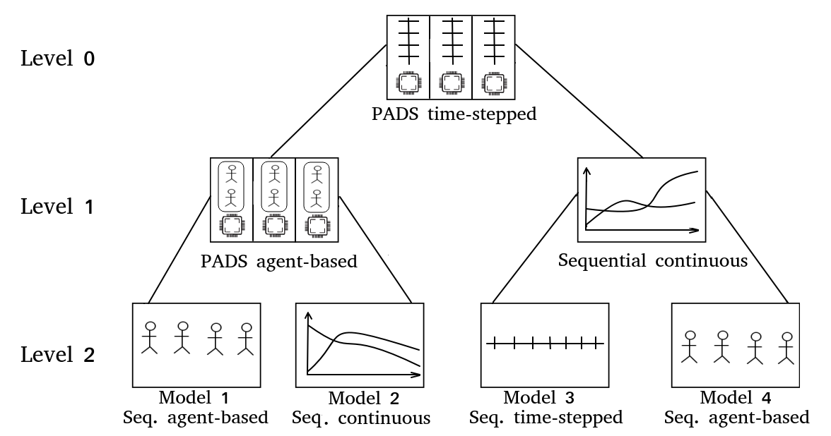
Figure 1: Multilayer model using different types of sub-models and execution policies.

Figure 1 shows a schematic representation of a multilevel model. Different types of models can coexist in the hierarchy (e.g., time-stepped, agent-based, continuous), as well as different execution policies (sequential or parallel/distributed). The role and type of each component of the hierarchy, and the structure of the whole hierarchy, are model-specific. In general, we expect that sub-models that are lower in the hierarchy (i.e., towards the leaves) are more detailed than those at the top (towards the root). It may also be possible that intermediate nodes act as pure coordinators of their children, for example executing them in parallel if possible. The hierarchy does not need to be static, either: a node might spawn sub-models when needed, for example to ”focus” on some interesting emerging pattern that requires detailed study.

We can therefore classify each sub-model across the following three dimensions:

• Type of model (continuous, discrete, mixed): this attribute refers to the representation of time.

• Execution policy (sequential or parallel): this attribute tells how a sub-model is executed.

• Level of detail (low, high, adaptive): this attribute refers to the amount of state variables that are used to represent the state of a sub-model.

Advantages

Multilevel models provide various benefits. A complex model built upon independent and reusable blocks might be faster to develop. From the software engineering point of view, each building block can be developed independently, or taken from a library of existing models that have already been validated, therefore saving considerable time (however, integration tests still need to be performed).

A multilevel structuring favors the parallel execution of sub-models that have no inter-dependencies. Simulation of spatially-located entities (situated agents) naturally leads to some form of spatial decomposition, where the simulated space is partitioned across different simulators. If the partitions are independent, some ”cheap” parallelism can be achieved by simply running the sub-models on different execution units (processors or cores). Problems arise if entities, e.g., those situated along the border of different partitions, need to interact. In these cases, it is sometimes possible to let the higher-level model take care of these interactions. Individual sub-models might also be natively capable of parallel execution, e.g., because they have been built upon a parallel/distributed framework [16].

Challenges

Multilevel modeling poses several challenges, some of which are still being investigated by the M&S research community. First and foremost, identifying an ”optimal” partitioning – for some suitable definition of ”optimal” – can be difficult. As already said, models that exhibit a spatial structure naturally lead to partitioning the simulated space into connected, non-overlapping regions handled by different sub-models. Even in those simple scenarios, the partitioning problem remains nontrivial [17].

The interaction among different models is a major issue. Although standard interfaces for interoperation across simulators have been proposed [18], they are quite large and cumbersome to implement. A more lightweight approach is to use wrappers file to (i) schedule the execution of the various components, (ii) manage the I/O operations and the exchange of information among the various tools and (iii) ensure consistency of data and state variables.

During the execution of a model, it is often necessary to use one or more streams of (pseudo-)random values. It is common practice to generate pseudo-random numbers from one initial seed to ensure the repeatability of the results. In a parallel or distributed setting, each model has its own random stream. It is therefore necessary to ensure that (i) the random streams do not overlap, i.e., the initial seeds (or the pseudo-random generator) are chosen so that the random streams are independent, and (ii) the result of the multilevel model is not affected by the order in which the sub-models are executed.

Implementation

We now describe a possible realization of multilevel MS, focusing our attention on human mobility. The choice of this application area is motivated by its increasing relevance, e.g., to study the propagation of infectious diseases, to investigate better and ”smarter” transportation systems, or to fight pollution by reorganizing the way people commute to work or study.

Traditionally, human mobility has been studied using either agent-based or continuous models based on ODEs [19]. Agent-based models allow developers to accurately describe the behaviour of the actors involved. ODE-based models describe the aggregate behavior of a possibly large number of agents by taking into consideration ”average” behaviors. ODE-based models are simpler (and possibly less accurate, particularly when there is a non-negligible probability that agents deviate from the average behavior), and can be evaluated much more efficiently because their performance is independent from the number of individuals.

The easiest way to implement an agent-based simulation is to manage the time discretely, in order to facilitate the coordination and the interactions among the agents, which occur in certain time-steps. On the other hand, ODE models are continuous. Coupling discrete and continuous models can be problematic; we employ the standard solution of considering the execution of the continuous sub-models as time intervals that stretch inside the sorted list of events of the discrete models. If a discrete model $D$ has a continuous model $C$ as a sub-model, then $D$ starts the execution of $C$ when needed (say, at simulated time $T_{n}$). $C$ is configured to compute its state up to a simulated time that does not exceed the instant $T_{n+1}$ of the next event scheduled for $D$. Therefore, the result of the sub-model $C$ is made available to $D$ at its next time step. A similar mechanism is used if $C$ has $D$ as sub-model: the caller executes the callee up to a future time that does not exceed the minimum of the duration of the continuous phenomena and the time instant of the next discrete event.

To demonstrate the feasibility of a multilevel approach in the context of human mobility, we have developed a prototype framework based on LUNES [20], NetLogo [21] and custom-built compartmental models based on ODEs. In our prototype implementations, we use JSON-formatted data stored in temporary files to exchange information between models.

The  Large Unstructured NEtwork Simulator (LUNES) is a time-stepped agent-based simulator developed by Parallel and Distributed Simulation Research Group of the University of Bologna [22]. The tool provides a scalable and customizable simulation environment where users can define the behavior of the simulated entities and the data that is exchanged between agents. The software relies on the GAIA/ARTÌS middleware [17], which manages communication between logical processes, supporting parallel and distributed execution, migration of simulated entities, and load balancing both for computation and communication.

NetLogo is a multi-agent modelling environment based on the Logo programming language. NetLogo provides an integrated graphical environment to develop, execute and debug agent-based simulations. NetLogo models are built around turtles (i.e., situated agents) that can move around 2D or 3D space, and patches representing portions of space that do not move but can hold location-specific state data. NetLogo supports real-time plotting and graphing facilities to display metrics of interest in real time. NetLogo also supports a form of multilevel modelling through the LevelSpace extension that allows modelers to construct multilevel agent-based models within the NetLogo modeling environment [23]. LevelSpace allows the execution and management of multiple models in parallel. However, execution of models of different types (e.g., a continuous model within NetLogo) is not supported natively, since the language does not provide a native way to call external applications. This problem can be solved by launching NetLogo through pyNetLogo [24], a Python interface to NetLogo, allowing the developers to start a NetLogo model and to call its functions from a python script; execution of sub-models is then delegated to pyNetLogo rather than NetLogo itself.

Finally, the custom-built continuous models are based on the classic compartmental models, where the population is labelled with a unique feature, and where usually a set of ordinary differential equations defines the transition rule between compartments. This approach is widely used in epidemiology [25]. In our use cases, we developed the compartmental models in Python, employing the scipy library [26] to manage the differential equations.

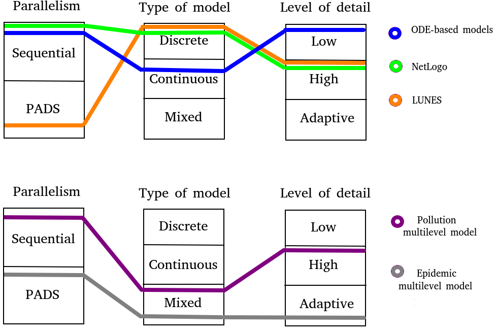
Figure 2: Top: Classification of the simulators used in the case studies. Bottom: classification of the models used in the case studies.

The top of Figure 2 classifies the building blocks above (NetLogo, LUNES and the scipy continuous model) with respect to the taxonomy introduced at the beginning of this section. NetLogo is a sequential, discrete simulator that is suitable for implementing detailed models, since the behavior of each agent (turtle, in NetLogo terminology) can be accurately programmed. LUNES is a parallel discrete simulator that, like NetLogo, allows very detailed system specifications by programming the behavior of agents using the C language. Finally, our custom continuous model provides coarse systems specifications using a set of Ordinary Differential Equations.

The bottom of Figure 2 classifies the two case studies that will be described in the next Section. The case studies implement simple multilevel models to analyze pollution due to different urban transportation strategies, and the diffusion of an epidemic. Both are mixed models since continuous and discrete simulators are used at different levels. The pollution case study is slightly more detailed and uses a sequential execution policy for all levels, while the epidemic model makes use of PADS techniques with the ability to dynamically tune the LoD at run-time.

IV Case Studies

In this section we describe two case studies that demonstrate the multilevel methodology described above and whose structuring is schematized in Figure 3. The case studies are not intended to be accurate or realistic; they are intended only to demonstrate that multilevel models can be ”natural” description of scenarios involving human mobility, and how multilevel models can be implemented in practice. To foster the reproducibility, all the source code used in this performance evaluation is freely available on https://github.com/luca-Serena/Multilevel-use-cases with a Free Software license.

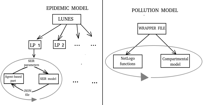
Figure 3: Rationale of the multilevel models for our use cases.

IV-A Epidemic Modeling

The first case study is the simulation of an epidemiological scenario. The model employs two levels, one based on LUNES and in charge of describing the mobility of individuals, and the other based on a continuous SEIR model describing the diffusion of the epidemic through time. A model like this could be used to evaluate the effectiveness of mobility restrictions to limit the diffusion of an epidemic. For example, we might compare no-lockdown, full lock-down, or restrictions based on the job of the individuals where only essential workers (e.g., healthcare personnel, food chain employees, bus drivers) were allowed to leave their homes.

We consider a non-fatal contagious disease for which permanent immunity is gained after contagion or immunization. The  Susceptible, Exposed, Infected, Recovered (SEIR) model [27] is a compartmental model where individuals are partitioned into four categories:

• Susceptible: individuals that may contract the disease. This is the initial state for all the individuals except for a single infected individual, the ”patient zero”.

• Exposed: individuals that contracted the disease but are not yet experiencing symptoms.

• Infected: individuals that contracted the disease and are experiencing symptoms.

• Recovered: individuals that developed immunity.

The dynamics of the SEIR model is governed by the following set of differential equations:

$$\left\{\begin{aligned} \frac{dS}{dt}&=-{\beta IS},\\[6.0pt] \frac{dE}{dt}&=\beta IS-\sigma E,\\[6.0pt] \frac{dI}{dt}&={\sigma E}-\gamma I,\\[6.0pt] \frac{dR}{dt}&=\gamma I\end{aligned}\right.$$ (1)

where $S$, $E$, $I$ and $R$ are the number of Susceptible, Exposed, Infected and Recovered individuals, respectively, $\beta$ is the infection rate, $\gamma$ is the recovery rate and $\sigma$ is related to the probability of transmission of the disease.

We entrust LUNES to model the mobility of agents, where each agent has a position and an epidemiological status; it should be noted that, for more realistic results, more information such as age, known health problems, mobility habits or vaccination status can be attached to agents. We assume that the model consists of several cities; the population density is higher inside a city, and agents also tend to move within their own city. Model parameters are the number of cities and their population, the mobility rates describing how often people move between cities, and the lockdown policies employed in each city. For each city, we create a software entity called the ”local coordinator”, which is a special simulated entity that has the task of aggregating the state of all individuals in the city and executing the continuous model.

The simulation starts with the launch of LUNES, which deals with the initialization of the virtual environment. In the setup phase, all the simulated entities are labelled as susceptible, with a single random individual chosen as the ”patient zero”. Each agent has a home location (the city where the associated individual resides), and an occupation that reflects the frequency of movement and whether the individual can be classified as an ”essential worker”.

After the setup phase, the following tasks are performed:

• The agents send their epidemiological status to the local coordinator associated with their location (city).

• The coordinators aggregate the data and compute the number of individuals in each epidemiological state (susceptible, infected, …).

• The coordinators check if the number of infected individuals is above the threshold for triggering lockdown policies, possibly restricting the mobility; thereafter, the SEIR model is executed using the aggregate values computed above. The various continuous models are executed in parallel.

• The coordinators, based on the results of the SEIR model, give instructions to the simulated entities on how to update their epidemiological status.

• Finally, some individuals are moved to a different city with a certain probability $p$.

Mobility restrictions have two effects in our model: constraining the flow of people moving between different areas, and reducing the contagion rate inside the cities. The model can be made adaptive, for example changing the parameters of the continuous model such as the accuracy of the ODE solver by reducing the integration time-steps. Indeed, we may want to increase the accuracy during the critical phases of the outbreak when the number of infected individuals rapidly grows. Also the infection rate could change over time, e.g., because once the infection is detected, mobility restrictions could lead to a lower pathogen diffusion rate.

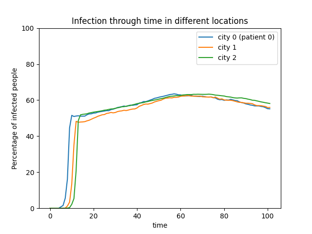
(a) Number of infected people vs
time in different cities.

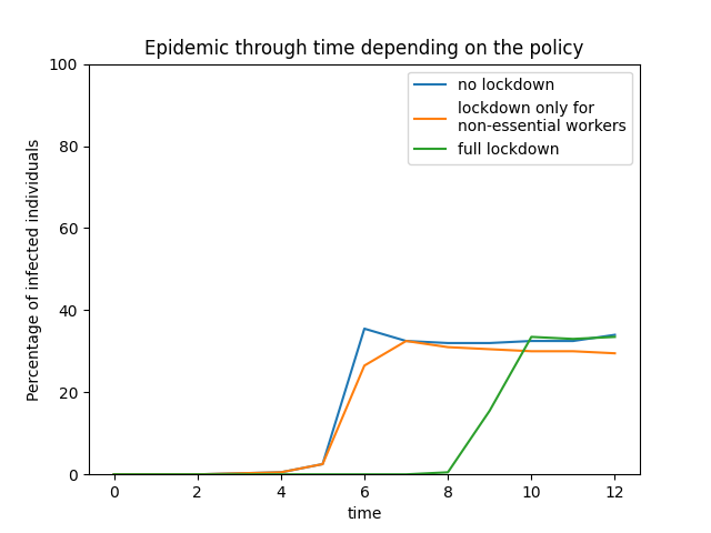
(b) Diffusion of the epidemic in a
location depending on restrictions.

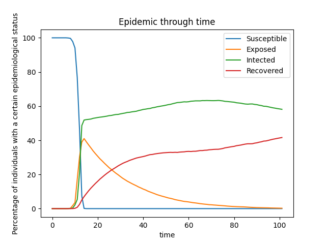
(c) Number of individuals in each state
as a function of time.

Figure 4:

Figure 4(a) shows that the disease propagates rapidly outside the city of origin. In fact, even assuming that infected people are not allowed to move outside their home city, exposed individuals still have no constraints in mobility, and therefore they will unknowingly diffuse the disease. Figure 4(b) shows that limiting the mobility introduces a delay in the propagation of the epidemic, but the global impact of the epidemic does not change. Finally, Figure 4(c) displays the progress of the epidemic inside a single location.

	3 Locations	6 Locations
1000 SEs	50.1 sec	75.7 sec
10000 SEs	49.9 sec	76.3 sec

TABLE I: Execution time depending on the number of simulated entities and locations. Tests performed on a PC with an 11th gen. Intel Core i5 processor with 16 GBs of RAM running GNU/Linux Ubuntu 20.04.4

From a performance point of view, as shown in Table I, the population size has a small impact in terms of execution time, since it depends mostly on the solution of the differential equations. On the other hand, the number of locations has a direct influence on the performance, since despite the greater parallelization level (under the assumption of using a logical process for each location) more SEIR models need to be executed, leading to higher time and memory consumption.

IV-B Green Mobility to Reduce Pollution

The second use case is a model that aims at estimating the amount of pollutants released into the atmosphere under different vehicular mobility policies. Vehicles are classified depending on the type of fuel: gasoline (the most pollutant), electricity (the less pollutant, although not completely pollution-free since part of the electricity is still produced using fossil fuels), and LPG (i.e., Liquefied Petroleum Gas) that lies somewhere in between.

We use NetLogo to represent the vehicles. When a vehicle (NetLogo turtle) moves on a patch (a cell of the discrete simulation space), the amount of pollution associated with that patch increases by a quantity that depends on the type of fuel used by the vehicle. Also, every patch propagates parts of its pollution to the neighboring patches, to simulate the diffusion of pollutants in the atmosphere. Periodically, a continuous model is executed to update the type of vehicles. The continuous model describes the effect of (dis-)incentives that might be put in place in order to favor some types of fuel over the others. We defined an ad-hoc compartmental model based on the following set of differential equations:

$$\left\{\displaystyle{\begin{aligned} \frac{dP}{dt}&=-\beta P-\sigma P,\\[6.0pt] \frac{dL}{dt}&={\beta P-\gamma L},\\[6.0pt] \frac{dE}{dt}&=\sigma P+\gamma L\end{aligned}}\right.$$ (2)

where $P$, $L$ and $E$ are the number of petrol, LGP and electric vehicles, respectively, and $\beta$, $\sigma$ and $\gamma$ are the transition rates from petrol to LGP, from petrol to electric and from LGP to electric. For the sake of simplicity, we do not allow other types of transitions, although they could easily be included by extending the equations appropriately.

We assume that electric vehicles do not emit pollutants locally but do contribute slightly to global pollution, since production of energy may have environmental costs. To model this phenomenon, we periodically increase the pollution of all patches (even those without any vehicle) by some small quantity that depends on the number of electric vehicles in the model.

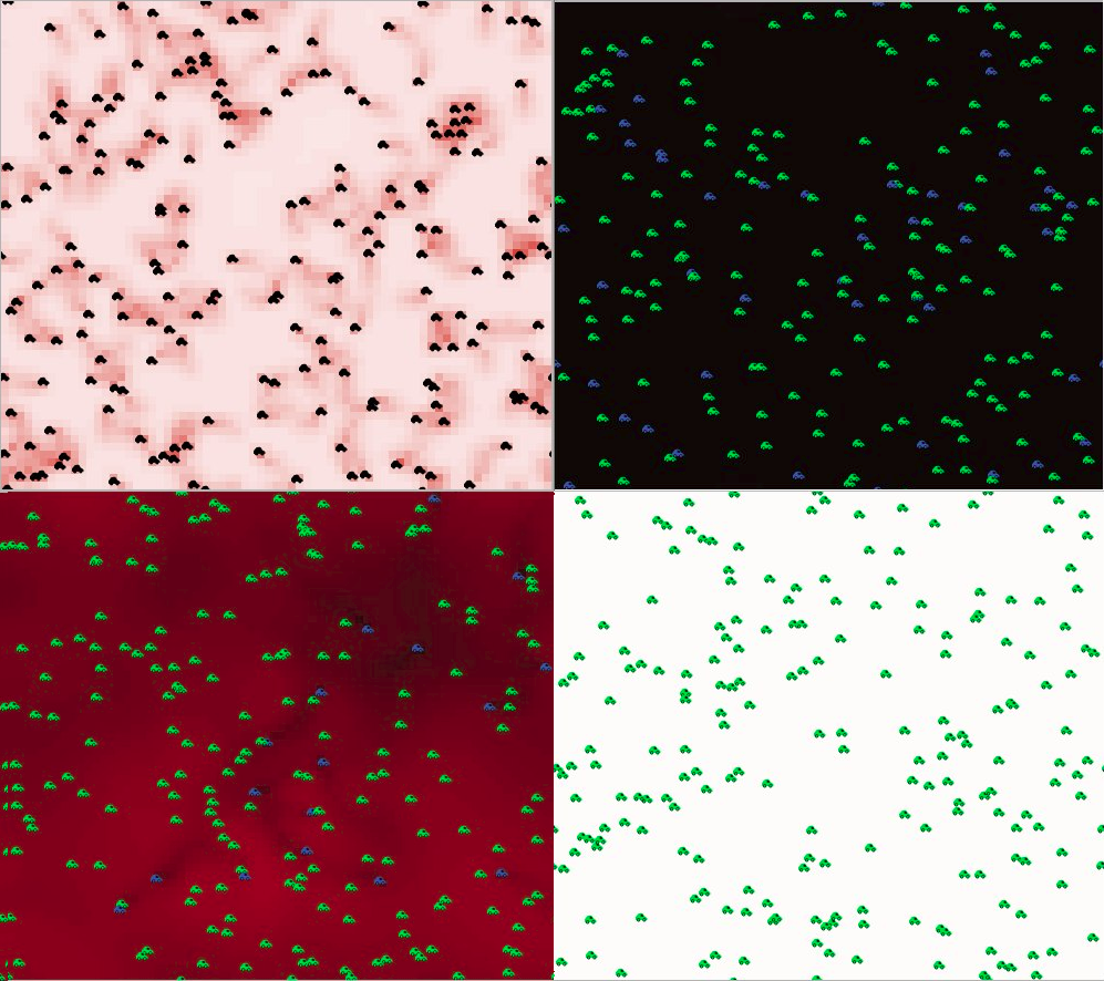
Figure 5: Four snapshots of the NetLogo model at different times. Green turtles = electric vehicles. Blue turtles = LGP-based vehicles. Black turtles = gasoline vehicles. White patches = no pollution. Red patch = medium pollution. Black patches = maximum pollution (best viewed in color).

Other important model parameters are (i) the pollution produced locally by the vehicles (higher for petrol, lower for LGP; electric vehicles produce no local pollution but do contribute to global pollution), (ii) the ”evaporation rate”, which is the amount of pollutants that vanish at each time-step, e.g., because it decays to inert stuff or is somewhat captured, and (iii) the initial number of vehicles of each type. Figure 5 shows a screenshot of the NetLogo model, where colors represent the type of vehicles and the amount of pollution in each patch.

To manage the execution of the simulation, we use a wrapper file that launches NetLogo through the pyNetLogo library and then runs both NetLogo and the continuous model with the correct parameters. After the setup phase, the execution proceeds as follows:

• each vehicle moves in a random direction, spreading pollutants over the visited cells;

• pollutants diffuse in the atmosphere according to the model parameters;

• every $n$ steps, where $n$ is a model parameter, the continuous model is called to update the types of vehicles that are moving in the simulation.

According to the chosen parameters, where we assume that vehicles running petrol emit as twice pollutants with respect to LPG-based vehicles and where electricity is produced using zero-emission technologies, then the model converges towards a zero pollution situation, meaning that the pollution produced at each time-step is lower than the evaporation-rate. In fact, in our scenarios, the pollution level initially grows, but the curve is gradually reverted with the switch towards ”greener” means of transport. If we assume that the production of electricity is not exactly zero-emission, the model converges towards zero pollution more slowly, as long as $\mathit{NumOfVehicles}\times\mathit{electricityProductionPollution}<\mathit{EvaporationRate}$.

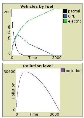
Figure 6: NetLogo real-time plots showing the evolution of the level of pollution and the types of vehicles through time.

The time required to converge towards a low pollution state is dependent on the incentives to purchase less polluting vehicles, as shown in Figure 6. Under the reasonable assumption that the vast majority of vehicles are initially petrol-based, pollution grows rapidly at the beginning of the simulation, but then starts decreasing as more vehicles are replaced with better ones. Figure 5 shows how the model progresses over simulated time. Initially (upper left) petrol-based vehicles start to release pollutants. At simulation step $1000$ (upper right) pollution peak is reached, and all patches are at their maximum contamination level. At simulation step $2000$ (lower left) most of the vehicles have been replaced with electric ones, and the environment is getting cleaner. Finally, at simulation step $3000$ (lower right) all the patches reached their minimum pollution level as the green transition is completed.

V Conclusions

In this paper we provided some preliminary evidence that multilevel modelling can be proficiently employed in different simulation scenarios, in particular those involving human mobility. Despite some issues regarding the consistency across different models and the need to coordinate the execution of the various sub-components, there are indications that the benefits of a multilevel approach outweigh the cons. First of all, multilevel modeling simplifies the development phase (i.e., different developers implementing separately a different component of the model) and allows faster execution (i.e., certain sub-models might be launched in parallel). Second, it enables the integration of existing tools, exploiting already-tested and task-specific code allowing for faster and more accurate software development. Finally, describing a complex system at different levels of detail might bring advantages both computationally (representing a whole system at a micro level could lead to undue computational effort) and semantically (having different descriptions of a system).

To support the above points, we provided two simple prototype models describing the diffusion of a contagious disease, and the diffusion of pollutants caused by vehicular traffic. In both instances, agent-based simulators and continuous models have been combined, exchanging information through JSON files. Our prototyping efforts show that a multilevel methodology has a great potential for allowing faster development of complex models that can be easily extended to carry out more thorough and complex investigations.

References

- [1] G. D’Angelo, S. Ferretti, and V. Ghini, “Multi-level simulation of internet of things on smart territories,” Simulation Modelling Practice and Theory (SIMPAT), vol. 73, 2017.
- [2] R. Sargent, J. Mize, D. Withers, and B. Zeigler, “Hierarchical modeling for discrete event simulation (panel),” in Proceedings of 1993 Winter Simulation Conference - (WSC ’93), 1993, pp. 569–572.
- [3] G. D’Angelo and M. Marzolla, “New trends in parallel and distributed simulation: From many-cores to cloud computing,” Simul. Model. Pract. Theory, vol. 49, pp. 320–335, 2014.
- [4] W. E, Principles of Multiscale Modeling. Cambridge University Press, 2011.
- [5] P. M. Tarwater and C. F. Martin, “Effects of population density on the spread of disease,” Complexity, vol. 6, no. 6, pp. 29–36, 2001.
- [6] R. A. Sahner, K. S. Trivedi, and A. Puliafito, Performance and Reliability Analysis of Computer Systems An Example-Based Approach Using the SHARPE Software Package. Springer Science & Business Media, 2022.
- [7] R. A. Sahner and K. S. Trivedi, “Reliability modeling using sharpe,” IEEE Transactions on Reliability, vol. 36, no. 2, pp. 186–193, 1987.
- [8] M. Martcheva, N. Tuncer, and C. St Mary, “Coupling within-host and between-host infectious diseases models,” Biomath, vol. 4, no. 2, p. 1510091, 2015.
- [9] L. Wang, Y. Zhang, Z. Wang, and X. Li, “The impact of human location-specific contact pattern on the sir epidemic transmission between populations,” International Journal of Bifurcation and Chaos, 2013.
- [10] S. Chang, E. Pierson, P. W. Koh, J. Gerardin, B. Redbird, D. Grusky, and J. Leskovec, “Mobility network models of covid-19 explain inequities and inform reopening,” Nature, vol. 589, no. 7840, pp. 82–87, 2021.
- [11] K. Peng, Z. Lu, V. Lin, M. R. Lindstrom, C. Parkinson, C. Wang, A. L. Bertozzi, and M. A. Porter, “A multilayer network model of the coevolution of the spread of a disease and competing opinions,” Mathematical Models and Methods in Applied Sciences, 2021.
- [12] E. Cristiani, B. Piccoli, and A. Tosin, “Multiscale modeling of granular flows with application to crowd dynamics,” Multiscale Modeling & Simulation, vol. 9, no. 1, pp. 155–182, 2011.
- [13] J. J. Olstam and A. Tapani, Comparison of Car-following models. Swedish National Road and Transport Research Institute Linköping, 2004, vol. 960.
- [14] D. Ni, “Multiscale modeling of traffic flow,” Mathematica Aeterna, vol. 1, no. 1, pp. 27–54, 2011.
- [15] R. Ekyalimpa, M. Werner, S. Hague, S. AbouRizk, and N. Porter, “A combined discrete-continuous simulation model for analyzing train-pedestrian interactions,” in 2016 Winter Simulation Conference (WSC). IEEE, 2016, pp. 1583–1594.
- [16] R. M. Fujimoto, Parallel and Distributed Simulation Systems. Wiley-Interscience, 2000.
- [17] G. D’Angelo, “The simulation model partitioning problem: an adaptive solution based on self-clustering,” Simulation Modelling Practice and Theory (SIMPAT), vol. 70, pp. 1 – 20, 2017.
- [18] “IEEE Standard for Modeling and Simulation (M&S) High Level Architecture (HLA)–Framework and Rules,” IEEE Std 1516-2010 (Rev. of IEEE Std 1516-2000), pp. 1–38, 2010.
- [19] H. Barbosa, M. Barthelemy, G. Ghoshal, C. R. James, M. Lenormand, T. Louail, R. Menezes, J. J. Ramasco, F. Simini, and M. Tomasini, “Human mobility: Models and applications,” Physics Reports, vol. 734, pp. 1–74, 2018, human mobility: Models and applications.
- [20] G. D’Angelo and S. Ferretti, “Adaptive parallel and distributed simulation of complex networks,” Journal of Parallel and Distributed Computing, vol. 163, pp. 30–44, 2022.
- [21] S. Tisue and U. Wilensky, “Netlogo: A simple environment for modeling complexity,” in International conference on complex systems, vol. 21. Boston, MA, 2004, pp. 16–21.
- [22] G. D’Angelo, S. Ferretti, and L. Serena, “Parallel And Distributed Simulation (PADS) Research Group,” http://pads.cs.unibo.it, 2022.
- [23] A. Hjorth, B. Head, C. Brady, and U. Wilensky, “Levelspace: A netlogo extension for multi-level agent-based modeling,” Journal of Artificial Societies and Social Simulation, vol. 23, no. 1, 2020.
- [24] M. Jaxa-Rozen and J. H. Kwakkel, “Pynetlogo: Linking netlogo with python,” Jasss, vol. 21, no. 2, 2018.
- [25] F. Brauer, “Compartmental models in epidemiology,” in Mathematical epidemiology. Springer, 2008, pp. 19–79.
- [26] T. E. Oliphant, “Scipy tutorial,” 2004.
- [27] M. Y. Li and J. S. Muldowney, “Global stability for the seir model in epidemiology,” Mathematical biosciences, vol. 125, no. 2, pp. 155–164, 1995.