Endogenous Fragility in
Opaque Supply Chains

Abstract

This paper investigates the role of supply chain unobservability in generating endogenously fragile production networks. In a simple production game, in which firms with imperfect information need to multisource to hedge against suppliers’ risk, firms underdiversify vis-à-vis the social optimum. The unobservability of suppliers’ relations is the driver behind this. In production networks where upstream risk is highly correlated and supplier relationships are not observable, the marginal risk reduction of adding an additional supplier is low, because this additional supplier’s risk is likely to be correlated to that of existing suppliers. This channel reduces firm incentives to diversify, which gives rise to inefficiently fragile production networks.

By solving the social planner problem, I show that, if the risk reduction experienced downstream resulting from upstream diversification were to be internalised by upstream firms, endogenous production networks would be resilient to most levels of risk. Furthermore, I show that the opaqueness of the supply chain yields less fragile but more inefficient production networks. Despite its stylised form, the model identifies the trade-off firms face when diversifying risk and isolates the mechanism that aggregates these decisions into a production network. Furthermore, it maps the conditions of the trade-off, such as expected profits of the firm or the pairing costs, to the properties of the production network.

In August 2020, hurricane Laura hit one of the world’s largest petrochemical districts, in the U.S. states of Louisiana and Texas. As polymer producers in the area were forced to halt production, up to 15% of the country’s polypropene (PE) and polypropene (PP) producers were unable to source polymer inputs, which in turn caused shortages across the economy ([22]). Such a widespread disruption raised awareness on the role suppliers’ correlation has in destabilising production networks and its importance in firms’ sourcing decisions. Yet, the structure of the supply chain is often opaque: firms do not observe sourcing relations beyond their immediate suppliers ([10]). In face of this opacity, how do producers make sourcing decisions? And, should we expect these sourcing decisions to yield resilient production networks?

In this paper, I study the role of supply chain opacity in determining firms’ sourcing decisions and, in turn, the consequences on the resilience of the production network. A widespread approach to mitigate risk is to diversify it by multisourcing. This practice consists of procuring the same inputs from multiple suppliers, sometimes redundantly ([18]). Yet, when deciding how many suppliers from which to source, a firm faces decreasing marginal benefits in risk reduction, because each additional supplier’s failure to deliver is increasingly likely to be correlated with that of the firm’s current suppliers. In the presence of marginal costs of sourcing, for example contractual costs or higher prices, the uncertainty behind the correlation of a firm’s potential suppliers might induce it to diversify risk less than socially optimal. The wedge between endogenous firm decisions and social optimality arises because downstream firms would be willing to compensate their suppliers for increased diversification of inputs. This underdiversification can generate aggregate fragility in production networks. To understand the relationship between the opacity of the supply chain, firms’ diversification decisions, and production network fragility, I study the properties of a stylised production game. In the equilibrium of the game, unobserved correlation among suppliers generates fragility via two channels. First, it directly introduces endogenous correlation in downstream firms’ risk, which amplifies through the production network. This increases the probability of cascading failures, in which the entire production network is unable to produce. Second, it indirectly affects firms’ decisions by reducing the expected marginal gain from adding a source of input goods. The latter channel leads to firms diversifying increasingly less, such that small shocks in the production of basal goods can generate cascading failures downstream.

The role that production networks play in determining economic outcomes has been long recognised. As far back as [1] (1), economists have studied how networks in production can act as aggregators of firm level activity. Following a foundational paper by 2 (2), which showed that the first order impact of a productivity shock to an industry is independent of the production network structure, macroeconomics has since de-emphasised this role ((16, p. 2)). However, more recently, 16 (16) illustrated how the structure of the production network can aggregate micro shocks via second order effects. Furthermore, the degree of competition in an industry also interacts with the production network to aggregate shocks, which can lead to cascading failures (15). Once established that production networks play a central role in aggregating shocks, two natural questions arise. First, which networks can we expect to observe, given that firm endogenously and strategically choose suppliers? Second, are these endogenous network formations responsible for the growth or fragility that large economies display? These questions fuelled a number of recent papers studying endogenous production network formation. Focusing on growth, 19 (19) show that endogenous production networks can be a channel through which firms’ increased productivity lowers costs throughout the supply chain and allows for sustained economic growth. In parallel, a vast literature dealt with studying the role of endogenous production networks and firm incentives in determining fragile or resilient economies. 11 (11) showed that in networks with strategic link formation, systemic endogenous fragility arises if the shocks experienced by firms are correlated. Later work, by 20 (20), shows that uncertainty in the time of production is crucial in determining whether production networks in equilibrium are sparse, hence fragile. Finally, 23 (23) illustrate how complexity in the production process can also be a key driver of endogenous fragility in production networks.

A less understood link is that between the opacity of the supply chain, how firms deal with it, and which consequences this has on the economy. 21 (21) studied the effect of uncertainty in endogenous production network formation on firms’ productivity and business cycles. They find that higher uncertainty can lead to lower economic growth. In contrast, this paper focuses on the role of uncertainty in generating endogenous fragility to cascading failures using a more stylised production network model, akin to that studied by 23 (23). In line with the existing literature, in the model small idiosyncratic shocks can be massively amplified. The degree of amplification depends on the equilibrium behaviour of firms. This phenomenon holds true in vertical economies producing simple goods. The novel theoretical contribution of this paper is to extend the analysis of production network formation to an opaque environment in which firms aim to minimise risk while accounting for correlation between suppliers. To do so, I develop a tractable analytical framework that describes the propagation of idiosyncratic shocks through the supply chain when firms take sourcing decisions endogenously in an imperfect information environment. The model describes the evolution of risk through the supply chain as a dynamical system over the depth of the production network. The social planner solution shows that endogenous fragility can impose large welfare losses. Importantly, these losses might be discontinuous: an arbitrary small increase in the correlation of risk among basal firms, can generate large welfare losses. Finally, I study a benchmark case without opacity, in which firms have full information. In this case, despite each individual firm being able to achieve smaller disruption risk, the production network is maximally fragile and there is a high probability of large disruptions.

The remainder of the paper is structured as follows. Section 1 discusses the assumptions on the supply chain disruptions, the problem of the firm, and establishes the results that allow the firm to make sourcing decisions. Section 2 derives the law of propagation of the disruption events through the production network. Section 3 establishes the firm’s optimal sourcing strategy and how this endogenously determines the fragility of the production network. These results are then compared, in Section 4, to the social planner solution to determine the welfare losses induced by the firm’s endogenous decisions. Finally, in Section 5, the role of opacity is isolated by solving the model under perfect information.

1 Model

1.1 Production Technology and the Firm Objective

Consider a vertical economy producing $K+1$ goods, indexed by $k\in\{0,1,\ldots K\}$. Each firm produces a single good and each good is produced by $m_{k}$ firms. Production of the basal good $k=0$ does not require any input, yet, it is at risk of random exogenous disruptions in the production process. A disrupted basal firm is unable to deliver its good as input to downstream producers. Each downstream good $k>0$ requires only good $k-1$ as input. If a firm producing good $k$ is unable to source its input good $k-1$, the firm is itself disrupted and hence unable to deliver downstream. In other words, the $i$-th firm producing good $k$, indexed by $(k,i)$, is able to produce if at least one of its suppliers is able to deliver, namely, not all of its suppliers are disrupted. To avoid being disrupted, the firm chooses which firms to source from, among the producers of its input good. Letting $\mathcal{D}_{k}$ be the random set of disrupted firms in layer $k$ and $\mathcal{S}_{k,i}$ the set of suppliers of firm $(k,i)$, we can say that $(k,i)\in\mathcal{D}_{k}$ if and only if all of its suppliers $(k-1,j)\in\mathcal{S}_{k,i}$ are in $\mathcal{D}_{k-1}$. I refer to the set of the firm’s suppliers $\mathcal{S}_{k,i}$ as its sourcing strategy. The disruption events are random and the probability that a firm is disrupted can be written as

$$P_{k,i}\coloneqq\mathbb{P}\big{(}(k,i)\in\mathcal{D}_{k}\big{)}=\mathbb{P}\big{(}\mathcal{S}_{k,i}\subset\mathcal{D}_{k-1}\big{)}.$$ (1)

Figure 1 illustrates this mechanism.

Figure 1: The supply chain is depicted in the left panel. The left firm is sourcing its input good from all three suppliers, $\mathcal{S}_{1}$, while the right firm only from the latter two, $\mathcal{S}_{2}$. As a disruption occurs, some upstream firms are unable to supply the input good (white box). Unlike the left firm, the right firm is unable to source its inputs and is hence disrupted.

If a firm is not disrupted, it obtains a profit $\pi$. Implementing a given sourcing strategy costs the firm $C\big{(}\left\lvert\mathcal{S}_{k,i}\right\rvert\big{)}$. The cost $C$ is assumed to be increasing in the number $\left\lvert\mathcal{S}_{k,i}\right\rvert$ of suppliers. The problem of firm $(k,i)$ is then to maximise the expected profit

$$\Pi_{k,i}(\mathcal{S}_{k,i})=\Big{(}1-\mathbb{P}\big{(}\mathcal{S}_{k,i}\subseteq\mathcal{D}_{k-1}\big{)}\Big{)}\;\pi-C\big{(}\left\lvert\mathcal{S}_{k,i}\right\rvert\big{)}$$ (2)

by picking a sourcing strategy $\mathcal{S}_{k,i}$. Before moving on with the solution of the model, it is useful to discuss the assumptions presented in this section. The production game is highly stylised: first, firms do not adjust prices but only quantities, such that failure to produce only arises in the case that no input is sourced; second, they are able to obtain profits by simply producing; third, contracting with new suppliers has a cost. There are both theoretical and empirical reasons behind these choices. Theoretically, a simpler model allows us to isolate the interplay between the variables of interest: correlation in the risk of suppliers, supply chain opacity, and the endogenous production network fragility. Empirically, these assumption capture well the rationale behind firms’ multisourcing. There is strong evidence that firms, first, when faced with supply chain shocks, adjust quantities rather than prices in the short run ([24, 25, 7, 13]), second, that production shutdowns can be extremely costly ([12, 3]), and third, that fostering relationships with suppliers is costly, but important in guaranteeing operational performance ([5]). The model establishes a link between these issues faced by firms when choosing a sourcing strategy and the fragility of the production network.

1.2 Opacity of the Supply Chain

The supply chain is opaque: firms cannot observe the sourcing decisions of their potential suppliers before making their own. Furthermore, firms do not know how risky individual basal producers are, nor how their risk is correlated. Yet, firms know the distribution from which the probabilities of disruption in the basal layer are drawn. To motivate this definition of opacity, recall the introductory example of hurricane Laura. A downstream firm producing PP, might not be able to trace back the production steps from its input to individual polymer producers in Louisiana or Texas, and, hence, the exact exposure of its production process to hurricanes. Yet, it can estimate the aggregate risk the polymer industry faces in the region. Given this information about the basal layer and their own depth $k$ in the production network, firms can derive the distribution of risk among their suppliers and make sourcing decisions based on it. By symmetry, the risk of two firms downstream sourcing from the same number of suppliers is ex-ante identical, albeit possibly correlated. The following two assumptions formalise this idea. Introduce

$$X_{k,j}\coloneqq\begin{cases}1&\text{ if }(k,j)\text{ is disrupted and}\\ 0&\text{ otherwise, }\end{cases}$$ (3)

and $\mathcal{P}_{0}$ the space of probability distributions over the basal disruption events.

Assumption 1.

Fix an arbitrary symmetric measure $\nu$ over $\mathcal{P}_{0}$, that is, $\nu$ is invariant under relabelling of basal firms. The probability distribution $\mathbb{P}_{0}$ of disruptions in the basal layer is sampled from $\nu$. I assume $\nu$ is observed by all firms, while $\mathbb{P}_{0}$ is hidden.

Going back to the example of polymer producers, under this assumption, downstream PP producers understand how hurricane risk can impact the production of their input good, via $\nu$, yet, they cannot estimate the risk that individual polymer producers face, nor how this risk is correlated, since they do not observe $\mathbb{P}_{0}$.

Assumption 2.

If there are multiple sourcing strategies that yield the same expected profit, the firm chooses one with equal probability.

Proposition 1.

Under these assumptions, in each downstream layer $k\geq 1$, disruption events

$$X_{k,1},X_{k,2},X_{k,3}\ldots X_{k,m_{k}},$$

are exchangeable, that is, their distribution is invariant under permutation.

Proposition 1, proven in Appendix B.1, asserts that, from the point of view of the firm, all suppliers are ex-ante equal, yet their risk might be correlated. Hence, the profit of the firm depends exclusively on how many suppliers it chooses, rather than which suppliers it chooses. Hence, a firm producing good $k$ can first infer the distribution of the number $D_{k-1}\coloneqq\left\lvert\mathcal{D}_{k-1}\right\rvert$ of disrupted firms among its potential suppliers and then choose the optimal number $s_{k,i}\coloneqq\left\lvert\mathcal{S}_{k-1,i}\right\rvert$ of firms from which to source its input good. Furthermore, by symmetry, all firms in layer $k$ choose the same number $s_{k}$ of sources, that is,

$$s_{k,i}=s_{k}\text{ for all }i.$$ (4)

As a result, the sourcing strategies $\mathcal{S}_{k,i}$ and $\mathcal{S}_{k,j}$ of any two firms $i$ and $j$ are such that their disruption probabilities $P_{k,i}$ and $P_{k,j}$ are identically distributed ([4, 6]).

2 Disruptions Propagation

Building on the mechanisms behind firms’ disruptions introduced above, this section studies how these disruptions propagate through the supply chain. To do so, I consider the case in which the number $m_{k}$ of firms in each layer $k$ grows large. To study the limit, it is first necessary to characterise how the sourcing relations $\mathcal{S}_{k,j}$ form as the number of firms in each layer increases.

Assumption 3.

As a new firm is introduced in layer $k$, it starts establishing relations with its $s_{k}$ suppliers. As soon as it pairs with a supplier, a new firm is introduced among the producers of its input good $k-1$, which, in turn, selects its sources. This procedure continues recursively until all firms realised their sourcing strategy $s_{k}$.

Indexing by $n$ the $n$-th step of this procedure, this section focuses on the limit as $n\to\infty$. Every new firm introduced in the basal layer has a disruption probability that is $\nu$-distributed, hence, the new firm is ex-ante identical to existing firms. This ensures that, as $n\to\infty$, Assumption 1 is satisfied and the downstream sourcing decisions $s_{1},s_{2}\ldots$ are unaffected. This, allows us to simply consider the problem of the representative firm in layer $k$.

To analytically characterise the disruption propagation through the production network, the only missing piece is the distribution $\nu$ of the disruption probabilities in the basal layer. As mentioned in the previous section, I assume that basal firms fail with a not necessarily independent probability $P_{0}$. We can model this by assuming that $P_{0}$ follows a Beta distribution.

Assumption 4.

The probability of a disruption in the basal layer follows

$$P_{0}\sim\nu_{0}\equiv\text{Beta}\text{ for all }j.$$ (5)

The Beta distribution allows to flexibly model shocks that might happen due to spacial or technological proximity of basal producers, which cannot be diversified. Consider, for example, how oil extraction plants must be located nearby oil reserves and are hence all subject to correlated weather shocks that might force them to shut down. In this case, despite the small expected probability that an individual firm is disrupted, as a hurricane is a rare occurrence, disruptions are highly correlated, as when a hurricane occurs most of them are disrupted. To keep track of the expected disruption probability and the correlation of risk through the layers, I introduce the following alternative parametrisation of the Beta distribution.

Definition 1.

Let $\mu$ and $\rho$ be respectively the mean and the overdispersion of a Beta distribution with shape parameters $\alpha$ and $\beta$, defined by

$$\mu\coloneqq\frac{\beta}{\alpha+\beta}\text{ and }\rho\coloneqq\frac{1}{1+\alpha+\beta}.$$ (6)

I write $Y\sim\text{Beta}(\mu,\rho)$.

Given Assumption 4, the following result links the probabilities of experiencing a disruption from upstream suppliers of $k$ to downstream producers $k+1$.

Definition 2.

A random variable $Y$ follows a BetaPower distribution, with mean $\mu$, overdispersion $\rho$, and power $s$ if it can be written as $Y=X^{s}$ where $X$ follows a Beta distribution with mean $\mu$ and overdispersion $\rho$.

Proposition 2.

If the disruption probability $P_{k}$ among suppliers of good $k$ follows a BetaPower distribution, so does the downstream probability $P_{k+1}$.

The proof is provided in Appendix B.2. Proposition 2 guarantees that the distribution of disrupted firms will remain in the same distribution family as risk amplifies through the production network. This result allows us to describe disruption propagation in the supply chain by mapping the evolution of the parameters $\mu_{k}$ and $\rho_{k}$ through the layers. Furthermore, it allows firms to estimate $\mu_{k}$ and $\rho_{k}$ and use this to determine the optimal sourcing strategy $s_{k+1}$. It is useful at this point to give an interpretation of $\mu_{k}$ and $\rho_{k}$ in the context of our model. The parameter $\mu_{k}$ is the average number of disrupted firms. The parameter $\rho_{k}$ tracks the degree of correlation in the disruption of firms operating in layer $k$. I illustrate this in Figure 2. This figure shows the distribution of the disruption probability $P_{k+1}$ among downstream firms in the case the firm has a single supplier (dotted lines) or two suppliers (solid line). For low overdispersion, $\rho_{k}=0.01$, the suppliers’ disruptions are weakly correlated and the downstream disruption probability is concentrated around the average $\mu_{k}$. If firms contract an additional supplier, the distribution of failures decreases and remains concentrated around the average. As $\rho_{k}$ increases, the suppliers’ disruption events become more correlated and the downstream disruption probabilities become fat-tailed, that is, a significant fraction of firms is likely to be disrupted and, as a consequence, diversification is ineffective. If firms contract an additional supplier, risk decreases, but a large probability of disruptions remains.

Figure 2: Distribution of disruption probabilities of downstream firms for different levels of upstream correlation $\rho_{k}$, in the cases of single sourcing (dotted) and multisourcing (solid). In both cases $\mu_{k}=\frac{1}{2}$.

Having established the link between the disruptions of layer $k$ to layer $k+1$, I now turn to the analysis of how these propagate through the whole supply chain, before studying how firms make decisions endogenously. The following result recursively connects downstream distributions with upstream sourcing decisions and initial conditions.

Proposition 3.

The average number of disrupted firms between one layer $k$ and the next $k+1$ depends on the sourcing strategy $s_{k+1}$ via

$$\mu_{k+1}=\eta(s_{k+1},S_{k})\;\mu_{k},$$ (7)

where $S_{k}\coloneqq\prod^{k}_{j=1}s_{j}$ is the diversification level up to layer $k$ and $\eta$ is the risk reduction factor, which is given by

$$\begin{split}\eta(s_{k+1},S_{k})&=\left(\mu_{0}\frac{1-\rho_{0}}{\rho_{0}}+S_{k}\right)^{\overline{S_{k}s_{k+1}}}\Bigg{/}\left(\frac{1-\rho_{0}}{\rho_{0}}+S_{k}\right)^{\overline{S_{k}s_{k+1}}}\\ &=\left(\frac{\mu_{0}\;\frac{\rho_{0}}{1-\rho_{0}}+S_{k}}{\frac{\rho_{0}}{1-\rho_{0}}+S_{k}}\right)\left(\frac{\mu_{0}\;\frac{\rho_{0}}{1-\rho_{0}}+S_{k}+1}{\frac{\rho_{0}}{1-\rho_{0}}+S_{k}+1}\right)\dots\left(\frac{\mu_{0}\;\frac{\rho_{0}}{1-\rho_{0}}+S_{k}s_{k+1}-1}{\frac{\rho_{0}}{1-\rho_{0}}+S_{k}s_{k+1}-1}\right).\end{split}$$ (8)

This is proven in Appendix B.3. The risk reduction factor $\eta(s_{k+1},S_{k})$ governs how the firms’ choice $s_{k+1}$, the choices along the firms’ production chain $S_{k}$, and the basal conditions $\mu_{0},\rho_{0}$ affect the expected number of disruptions downstream. This interplay is illustrated in the following figures.

Figure 3 shows how the risk reduction factor varies with basal correlation $\rho_{0}$ for different sourcing strategies $s_{k}$, fixing the upstream diversification of $S_{k}=2$. If correlation $\rho_{0}$ in the basal layer grows, to obtain a given level of risk reduction $\eta$, firms producing good $k$ needs to source more suppliers. If $\rho_{0}\to 1$, diversification becomes impossible, as $\eta\to 1$ and $\mu_{k+1}\to\mu_{k}$ for any sourcing strategy $s_{k+1}$.

Figure 3: Risk reduction factor $\mu_{k+1}/\mu_{k}$ at different basal overdispersion levels $\rho_{0}$ and for different sourcing strategies $s_{k+1}$. $S_{k}=2$.

As the above, Figure 4 shows the response of the risk reduction factors to different levels of basal correlation, but instead of varying the strategy $s_{k}$ of the firm, it varies the level of upstream diversification $S_{k}$. For low levels of basal correlation $\rho_{0}$, more upstream diversification $S_{k}$ allows downstream producers to achieve lower risk with fewer suppliers. Yet, there is a level of basal correlation after which more diversification is detrimental for the downstream firm, as this high upstream diversification simply exacerbates tail-risk. This represents a crucial externality the upstream suppliers impose on downstream producers. For low level of correlation, sourcing downstream represents a positive externality downstream. This externality shrinks as correlation increases, until it becomes a negative externality. Section 4 explores the welfare consequences of this mechanism.

Figure 4: Risk reduction factor $\mu_{k+1}/\mu_{k}$ at different basal overdispersion levels $\rho_{0}$ and for different upstream diversification levels strategies $S_{k}$. $s_{k+1}=2.$

3 Firm Optimal Diversification and Competitive Equilibrium

The mechanics of disruption propagation, derived in the previous section, determine the firms’ risk diversification incentives and, as a consequence, their optimal sourcing strategy. This section derives such optimal strategies. Importantly, due to Proposition 1, all firms in a given layer are ex-ante identical and so is their optimisation problem. We can hence focus of the representative firm in layer $k+1$, choosing how many suppliers in layer $k$ to source from, based on the inferred distribution of their probability of experiencing a disruption event. This, in turn, is fully determined by the expected fraction of firms disrupted in the basal layer $\mu_{0}$, the correlation of such disruptions $\rho_{0}$, and the sourcing strategies of the representative firm upstream $\{s_{k},s_{k-1}\ldots s_{0}\}$. For illustration purposes in the next section, I assume firms face quadratic costs from contracting suppliers, with a fixed marginal cost $c$, such that expected profits can be written as

$$\Pi_{k}(s_{k})=\Big{(}1-\mathbb{E}\big{[}P_{k}\;|\;s_{k}\big{]}\Big{)}\pi-\frac{c}{2}s_{k}^{2},$$ (9)

The optimisation problem of the firm is to then choose the optimal sourcing strategy

$$s_{k}=\arg\max_{s\in\{0,1,2,\ldots\}}\Pi_{k}(s).$$ (10)

3.1 Limit Case: Uncorrelated Disruptions

Before turning towards the general framework, I first analyse a limit case in which suppliers’ risk is not correlated, $\rho_{0}\to 0$. This limit case allows to derive more results analytically, gives a useful interpretation of the incentives behind multisourcing, and allows to establish a benchmark against which to study the introduction of correlated shocks.

Proposition 4.

If risk among basal firms becomes uncorrelated $\rho_{0}\to 0$, disruption events in layer $k$ become independent and happen with probability

$$\mu_{k}=\mu_{k-1}^{s_{k}}=(\mu_{k-2}^{s_{k-1}})^{s_{k}}=\ldots=\mu_{0}^{S_{k}}.$$ (11)

Proof.

Follows immediately from $P_{k}\to\mu_{k}$ as $\rho_{0}\to 0$. ∎

Using the law of motion (11), we can rewrite profits (9) as

$$\Pi_{k+1}(s)=\big{(}1-\mu_{k}^{s}\big{)}\pi-\frac{c}{2}s^{2}.$$ (12)

Consider the marginal profits attained by adding an additional source of input goods,

$$\Delta\Pi_{k+1}(s)\coloneqq\Pi_{k+1}(s+1)-\Pi_{k+1}(s)=\mu_{k}^{s}(1-\mu_{k})\pi-c\left(s+\frac{1}{2}\right).$$ (13)

A firm with a given number of suppliers, contracts an extra supplier if doing so yields a positive expected marginal profit. Hence, the optimal number of suppliers $s_{k+1}$ is the smallest $s$ for which the expected marginal profit is negative $\Delta\Pi_{k+1}(s)<0$.

Definition 3.

Let $\tilde{s}_{k+1}$ be the unique root of $\Delta\Pi_{k+1}(s)$ over $[-1/2,\infty)$. I refer to this quantity as the “diversification incentive”.

Proposition 5.

The optimal sourcing strategy is given by $s_{k+1}=\left\lceil\tilde{s}_{k+1}\right\rceil$.

The proof of the uniqueness of $\tilde{s}_{k+1}$ and of Proposition 5 is given in Appendix B.4.1.

Corollary 5.1.

The firm does not source any input $s_{k+1}=0$ if the suppliers’ risk $\mu_{k}$ is greater than the threshold $\mu^{0}$,

$$\mu_{k}\geq\mu^{0}\coloneqq 1-\frac{c/2}{\pi}.$$ (14)

I refer to all levels of risk $\mu_{k}>\mu^{0}$ as “collapse regime”.

Proof.

Suppose firms do not source any inputs $s_{k+1}=0$. This implies that the marginal benefit of adding the first supplier is negative, namely $\Delta\Pi_{k+1}(0)\leq 0$, which yields the desired inequality. ∎

As expected, the diversification incentive $\tilde{s}_{k+1}$ and the optimal sourcing strategy $s_{k+1}$ are implicitly determined by the suppliers’ risk $\mu_{k}$ and the relative marginal cost of contracting a new supplier $\frac{c/2}{\pi}$. Figure 5 shows the optimal diversification incentive $\tilde{s}_{k+1}$ (solid line) and sourcing strategy $s_{k+1}$ (dotted line), given a suppliers’ level of risk $\mu_{k}$, for three different marginal costs ratios $\frac{c/2}{\pi}$. First, as the marginal pairing costs increase, the firm’s diversification incentives decrease. Second, higher levels of risk increase the diversification incentives of firms until a threshold is reached, after which, diversification incentives and, in turn, optimal diversification start decreasing. The concavity of the optimal sourcing strategy $s_{k+1}$ in the suppliers’ risk $\mu_{k}$, highlights a vicious cycle which is introduced in production networks when firm decisions are endogenised: after a certain level of risk, firms have less incentives to diversify, which, in turn, “flattens” the marginal expected profits downstream. This mechanisms can lead to endogenous fragilities in production networks.

Figure 5: $\tilde{s}_{k+1}$ (solid) and $s_{k+1}$ (dotted)

To illustrate the mechanism behind the endogenous fragility, we can combine the law of risk propagation (4) and the optimal firm sourcing (5) to obtain the risk dynamics in the production network,

$$\mu_{k+1}=\mu_{k}^{s_{k+1}(\mu_{k})}.$$ (15)

The recursive relation (15) maps risk from suppliers to firms throughout the production network, hence studying its properties allows to describe how risk propagates through the supply chain. Two natural questions arise: first, which levels of risk remain stable through the supply chain, that is, they are neither amplified nor dampened as one moves from suppliers to firms? Second, how are initial levels of risk mapped to these stable risk levels? The former can be answered by determining levels of risk $\bar{\mu}$ which are fixed points of equation (15). The latter by looking at the basin of attraction of such points.

Proposition 6.

The stable levels of risk $\bar{\mu}$ are all points satisfying

$$\frac{\bar{\mu}(1-\bar{\mu})}{3}\leq\frac{c/2}{\pi}.$$ (16)

Proof.

A steady state is attained if $\tilde{s}_{k+1}\leq 1$. This implies that the marginal benefit of multisourcing is not positive $\Delta\Pi_{k+1}(1)\leq 0$. This yields the desired inequality. ∎

Corollary 6.1.

For all basal risk levels $\mu_{0}$ larger than the critical threshold

$$\mu^{c}\coloneqq\frac{1}{2}+\sqrt{\frac{1}{4}-3\frac{c/2}{\pi}},$$ (17)

the endogenous supply chain is unable to diversify risk $\overline{\mu}=\mu_{0}$. I refer to this situation as “endogenous fragility”.

Figure 6:

Propositions 6 and 6.1 (proven in Appendix B.4.2) link the firms’ relative costs $\frac{c/2}{\pi}$ and the aggregate outcomes in term of production network risk. As relative marginal costs increase, the capacity of the production network to endogenously diversify basal risk $\mu_{0}$ decreases and firms’ underdiversification yields endogenous fragility. It is interesting to notice that, comparing the aggregate threshold $\mu^{c}$ with the firm shutdown threshold $\mu^{0}$ (Figure 6), for some levels of basal risk $\mu_{0}$, despite no firm shutting down production $\mu_{0}<\mu^{0}$, the production network as a whole is still unable to endogenously diversify risk $\mu_{0}>\mu^{c}$. This is true even in this special case, where firms’ risk is uncorrelated. In the next section, I introduce correlation risk $\rho>0$ and investigate how doing so changes the dynamics illustrated here.

3.2 Optimal Sourcing with Correlated Distributions

If disruption events are not independent, $\rho_{0}>0$, risk among suppliers throughout the production network is correlated, and firms’ optimisation incentives change. The firm problem (9) in layer $k+1$ is to choose the number of suppliers $s_{k+1}\in\{0,1,2\ldots\}$ that maximises the profits $\Pi$ given an upstream diversification $S_{k}$. The firm’s expected disruption probability is given by the expected probability of disruption among its suppliers $\mu_{k}$, scaled by a factor $\eta(s_{k+1},S_{k})$ (Proposition 3) which depends on the firm sourcing strategy. As in the limit case analysed in the previous section, the firm will increase diversification as long as the expected reduction in profits obtained by adding an additional supplier outweighs the costs of contracting that additional supplier. The expected marginal profits are given by

$$\Delta\Pi_{k+1}(s_{k+1})=\Big{(}\eta(s_{k+1},S_{k})-\eta(s_{k+1}+1,S_{k})\Big{)}\;\mu_{k}\pi-c\left(s_{k+1}+\frac{1}{2}\right).$$ (18)

As above, let $\tilde{s}_{k+1}$ be the “diversification incentive”, that is, the level of $s$ such that the marginal benefits and marginal costs of diversification are equal $\Delta\Pi_{k+1}(s)=0$. Since the marginal profits are strictly decreasing in the number of suppliers (see Appendix B.5), the firm will choose its optimal sourcing strategy as $s_{k+1}=\left\lceil\tilde{s}_{k+1}\right\rceil$ (Proposition 5). The correlation of risk among producers of its input good changes the firm’s incentives, as illustrated in Figure 7. In particular, as correlation increases, the firm needs to increase its sources to diversify risk. Yet, for large levels of correlation, the disruption of an additional source of the input good is likely correlated to a disruption among the firm’s existing suppliers, which reduces the firm’s multisourcing incentives. As disruptions among suppliers become perfectly correlated, $\rho_{k}\to 1$, the firm has no reason to multisource $\tilde{s}_{k+1}\to 0$.

Figure 7: Sourcing incentive (i.e. $s$ such that $\Delta\Pi_{k+1}(s)=0$) as suppliers’ risk correlation $\rho_{k}$ increases, for different values of suppliers’ risk, $\mu_{k}$

This result, proven in Appendix B.5, can be summarised as follows.

Proposition 7.

The sourcing incentive $\tilde{s}_{k+1}$ is concave in the overdispersion among suppliers $\rho_{k}$.

Corollary 7.1.

The optimal sourcing strategy is weakly concave in the overdispersion among suppliers $\rho_{k}$.

Proof.

If $\tilde{s}_{k+1}$ is concave in $\rho_{0}$ (Proposition 7), then taking the next largest integer $\left\lceil\cdot\right\rceil$ yields weak concavity. ∎

This result (7.1) introduces a channel through which the correlation of disruptions in the production networks, can generate externalities in the firms’ choices and yield an endogenously fragile production network. To analyse these ramifications, consider the recursive relation of risk $\mu_{k}$, when firms optimally source $s_{k+1}$ (parallel to equation 15),

$$\mu_{k+1}=\eta(s_{k+1},S_{k})\;\mu_{k}=\ldots=\prod^{k}_{j=0}\eta(s_{k+1-j},S_{k-j})\mu_{0}.$$ (19)

From the definition of $\eta$, it follows that downstream there exists a layer $\overline{k}$, such that, the distribution of disruptions is constant, or more formally, $s_{l}=1$ for all $l\geq\overline{k}$. Let $\overline{\mu}\coloneqq\mu_{K}$ be the stable downstream fraction of firms expected to fail downstream. Figure 8 illustrates this fraction for different levels of basal risk $\mu_{0}$ and overdispersion $\rho_{0}$ in a low (left) and a high (right) relative pairing cost regime. First, in both cases if $\rho_{0}\to 1$ there is no possible diversification since all firms are either disrupted or not, hence the disruption risk is constant across the production network $\overline{\mu}=\mu_{0}$, regardless of the sourcing strategy. Likewise, if risk among basal producers becomes independent, $\rho_{0}\to 0$, the problem converges to the limit case discussed in the previous section. Second, for a given level of basal correlation $\rho_{0}$, there is a critical threshold $\mu^{c}$ such that an arbitrary small increase in the initial risk level $\mu_{0}$ has a discontinuous effect in the fraction of downstream firms $\overline{\mu}$. As discussed in the previous section, this discontinuity is induced on the production network by the firms’ endogenous diversification incentives. As correlation increases, the maximum “diversifiable” level of basal risk, $\mu^{c}$, becomes smaller. This lowering critical threshold suggests that, when allowed to form endogenously, production networks display a tendency towards endogenous fragility. Importantly, the model suggests that cascading failures can be triggered not only by increases in basal risk $\mu_{0}$ but also by increases in basal correlation $\rho_{0}$, even as basal risk remains constant. This fragility, unlike the one studied by elliott_supply_2022 (elliott_supply_2022), is not induced by the structure of the production function, but rather arises endogenously due to the decreasing diversification motives of firms.

Figure 8: Surface of the downstream fraction of non functioning firms $\overline{\mu}$, given the initial condition $\mu_{0}$ and $\rho_{0}$ in a low (left) and a high (right) relative pairing costs regime.

4 Social Planner Problem

To establish a benchmark to which one can compare the competitive equilibrium analysed above, in this section I solve the model from the perspective of a social planner. The social planner attempts to, on the one hand, minimise the number of firms expected to fail, and, on the other, minimise the number of costly sourcing relations. To develop a useful benchmark, it is important to define a social planner problem that can be meaningfully compared to the decentralised firm’s problem. To do so, I make the following two assumptions.

Assumption 5.

The social planner knows the distribution of failure in the basal layer $P_{0}\sim\text{Beta}(\mu_{0},\rho_{0})$ and makes decision before $P_{0}$ is realised.

Assumption 6.

As in the firm problem, I consider the case $n\to\infty$. This allows the social planner to recursively, from the last layer $K$ upwards, assign suppliers $\mathcal{S}_{k,i}$ such that there are sufficiently many firms so that no two firms share suppliers $\mathcal{S}_{k,i}\cap\mathcal{S}_{k,j}=\emptyset$.

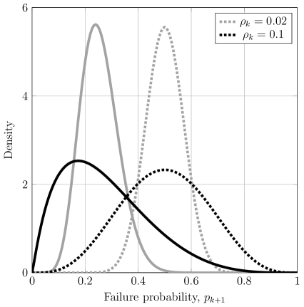
Figure 9:

To understand the intuition behind Assumption 6, consider the possible supplier overlap illustrate in Figure 9: if a supplier has multiple downstream clients (dashed box), the social planner can always rewire a link towards a supplier without downstream clients (solid box). By doing so, the social planner can “diversify away” all the correlation that arises due to the network structure. Hence, the only source of risk in the model is represented by the shutdowns experienced by firms in the basal layer, which happen with non-idiosyncratic probabilities $P_{0}$ (Assumption 5). Combining Assumptions 5 and 6, the social planner problem is then to maximise average expected payoffs

$$W(\{\mathcal{S}_{k,i}\})\coloneqq\frac{1}{K}\sum^{K}_{k=0}\lim_{n\to\infty}\frac{1}{m_{k}(n)}\sum^{m_{k}(n)}_{i=1}\Big{(}1-\mathbb{P}\big{(}\mathcal{S}_{k,i}\subset\mathcal{D}_{k-1}\big{)}\Big{)}\ \pi-\frac{c}{2}\left\lvert\mathcal{S}_{k,i}\right\rvert^{2},$$ (20)

by choosing a sourcing strategy $S_{k,i}\subseteq\{1,2,\ldots\}$ for each firm in each layer such that $S_{k,i}\cap S_{k,j}$ is empty for all $i,j$. The social planner problem can be further simplified by noticing that, given that all firms in layer $k$ are identical, if establishing an additional path from a firm in layer $k$ to a basal firm has positive marginal benefits, then it has positive marginal benefits for all firms in layer $k$ which share the same number of paths to basal firms. Hence, as in the decentralised firms’ problem, the social planner can choose the optimal number of sources in each layer, let the firms source at random, and finally disentangle any overlapping paths. Using this, the social planner problem can be formulated recursively, by letting $V_{k}$ be the maximal average welfare from layer $k$ to the last layer $K$. This can be recursively defined as

$$V_{k}(P_{k-1})=\max_{s_{k}}\left\{\left(1-\mathbb{E}\big{[}P_{k-1}^{s_{k}}\big{]}\right)\pi-\frac{c}{2}s_{k}^{2}+\mathbb{E}\big{[}V_{k+1}(R_{k})\big{]}\right\}$$ (21)

where the state $P_{k-1}\sim\text{BetaPower}(\mu_{0},\rho_{0},s_{1}s_{2}\ldots s_{k-1})$ is the fraction of disrupted firms, which evolves as

$$P_{k}=P_{k-1}^{s_{k}}.$$ (22)

The average welfare in layer $K+1$ is given by $V_{K+1}(P_{K})=0$, since firms in the last layer are never sources to other firms, and an initial state condition $P_{0}\sim\text{Beta}(\mu_{0},\rho_{0})$. This problem can be solved using standard backward induction techniques (see Appendix C). The optimum average social welfare (20) can then be written as

$$V_{1}(P_{0})=\max_{s_{1},s_{2},\ldots s_{K-1}}W(\{s_{1},s_{2},\ldots s_{K-1}\}).$$ (23)

Letting $\{s^{p}_{k}\}^{K}_{k=1}$ be the socially optimal sourcing strategies sequence and $\{\mu^{p}_{k}\}^{K}_{k=1}$ be the expected disruption in each layer given by such sourcing strategies, we can compute the change in downstream risk compared to the decentralised case (as illustrated in Figure 8). Figure 10 shows this difference $\overline{\mu}-\overline{\mu}^{p}$ for the same two cost regimes. On the one hand, when relative pairing costs are low (left panel), the social planner achieves marginally lower risk levels of downstream risk for most initial conditions. If initial basal correlation $\rho_{0}$ is sufficienctly large and basal risk $\mu_{0}$ is sufficienctly low, the firms overdiversify compared to the socially optimum $\overline{\mu}<\overline{\mu}^{p}$. On the other hand, if relative pairing costs are high (right panel), the differences between the social optimum and the competitive level of downstream risk are starker. First, for larger levels of basal risk $\mu_{0}$ and lower levels of basal correlation $\rho_{0}$ the firms overdiversify compared to the social optimum, $\overline{\mu}<\overline{\mu}^{p}$. Second, the social planner is able to diversify risk around the critical threshold $\mu_{c}$, $\overline{\mu}>\overline{\mu}^{p}$. This implies that the cascading failures that occur around the critical threshold are fully attributable to firms’ endogenous underdiversification motives.

Figure 10: Change in downstream expected failure probability between the firms’ $\overline{\mu}$ and the social planner $\overline{\mu}^{p}$ equilibrium, given different initial conditions $\mu_{0}$ and $\rho_{0}$ in a low (left) and a high (right) relative pairing costs regime.

The differences between the firms’ sourcing strategies and the social optimum generate welfare losses in the production network. Letting $W$ be the average firm profit in the decentralised case and $W^{p}$ be the average profit achieved by the social planner, in Figure 11 I show the welfare loss due to the firms’ diversification decisions $W-W^{p}$, in the high cost scenario ($\frac{c}{2}=0.02\pi$). The welfare loss is largest around the critical value $\mu^{c}$, where the production network suffer is endogenously fragile. At these levels of risk, firms’ upstream firms’ diversification incentives are weak, which creates large downstream resilience externalities. Crucially, both an increase in basal risk $\mu_{0}$ and an increase in basal correlation $\rho_{0}$ can generate discontinuous welfare losses.

Figure 11: Welfare loss of the decentralised equilibrium $W-W^{p}$, given different initial conditions $\mu_{0}$ and $\rho_{0}$.

5 The Role of Opacity

So far I assumed that firms cannot observe the realisation of the supply chain when making sourcing decisions. To understand how this assumption affects optimal decisions and fragility within the supply chain, I now analyse the supply chain under perfect information. The following assumption clarifies what is meant by perfect information in the context of the model.

Assumption 7.

In a regime of perfect information each firm firm $i$ in level $k$ is able to perfectly estimate the disruption probability of each potential supplier and the full correlation structure of the disruption events.

Under this perfect information regime, the firm can assign correct probabilities to its own disruption risk

$$\mathbb{P}\Big{(}\mathcal{S}_{k,i}\subset\mathcal{D}_{k-1}\Big{)}\text{ for all possible sourcing strategies }\mathcal{S}_{k,i}.$$

The firm can hence rank suppliers by the marginal reduction in risk they provide and source from the “safest” $s_{k}$ desired suppliers. As all firms downstream are ex-ante identical, the marginal benefits of diversification experienced by firm $(i,j)$ are the same as those of all other firms in layer $k$, which implies that, in equilibrium, all firms in layer $k$ will employ the same sourcing strategy, given that they are ex-ante identical. This outcome is beneficial for any single firm, but detrimental for the stability of the production network. The following to propositions formalise this.

Proposition 8.

Compared to the opaque scenario, for the same number of sources, firm $(k,i)$ is (weakly) less likely to be disrupted.

Proof.

Given the same number of sources, the firm with perfect information minimises its disruption risk with fewer constraints than in the opaque scenario. ∎

Proposition 9.

Under perfect information, the supply chain is maximally fragile: either all firms fail or none do.

Proof.

The equilibrium outcome under perfect information implies that a disruption in layer $k$ affects all firm simultaneously as they all share the same sources, namely

$$X_{k,i}=X_{k,j}\text{ for all }i\text{ and }j.$$

This, in turn, removes any diversification incentives downstream: a firm producing $k+1$ cannot diversify its risk by multisourcing, hence it will single source. ∎

Opacity has a dual role: on the one hand, it prevents firms from optimally choosing the best sourcing strategy; on the other hand, it mitigates endogenous fragility by forcing firm to diversify.

6 Conclusion

Risk diversification is a crucial determinant of firms’ sourcing strategies. In this paper, I show that firms endogenously underdiversify risk when they have incomplete information about upstream sourcing relations. This endogenous underdiversification generates fragile production networks, in which, arbitrarily small increases in correlation among disruptions between basal producers can generate discontinuously large disruptions downstream. I do so by deriving an analytical solution to a simple production game in which firms’ sole objective is to minimise the risk of failing to source input goods.

Despite its simple structure, the game identifies an important externality firms impose on the production network when making sourcing decisions: upstream multisourcing introduces correlation in firms’ risk, which reduces incentives to multisource downstream. This externality exacerbates the risk of fragile production networks. Furthermore, I show that a social planner can design production networks that mitigate fully this externality. A consequence of this result is that, in principle, it is possible to design a transfer mechanism that allows downstream firms to compensate upstream firms to internalise the diversification externalities. By analysing the welfare loss in competitive equilibrium, I show that there is a critical region of basal conditions where arbitrary small increases in suppliers’ correlation, even if the expected number of disrupted firms remains constant, can generate catastrophic downstream disruptions by altering downstream firm diversification incentives. This result illustrates how an increase in correlation among basal producers, for example due to widespread offshoring to the same country, can endogenously generate fragile production networks which have a large tail risk of disruption. Surprisingly, opacity plays a role in mitigating this effect, suggesting that if firms were to acquire information about the production network, despite the individual firm being better off, this could generate further endogenous fragility.

Appendix A Notation and Distributions

This appendix introduces standard notation and definitions that will be used throughout the following appendices.

For $x\in\mathbb{R}$ and $n\in\mathbb{Z}$, I denote the falling factorial as

$$x^{\underline{n}}\coloneqq\underbrace{x(x-1)(x-2)\ldots(x-(n+1))}_{n\text{ terms}}.$$ (24)

For non-integer exponents $s\in\mathbb{R}$, (24) can be extended as

$$x^{\overline{n}}\coloneqq\frac{\Gamma(x+n)}{\Gamma(x)},$$ (25)

where $\Gamma$ is the gamma function.

Two properties of the falling factorial that are used below but not proven are the additive property of the exponent

$$x^{\overline{n+m}}=x^{\overline{n}}(x+m)^{\overline{m}},$$ (26)

and that it is strictly increasing in its base

$$\frac{\partial x^{\overline{n}}}{\partial x}>0.$$ (27)

Appendix B Omitted Proofs

This appendix contains the proofs omitted from the paper.

B.1 Proof of Proposition 1

Proving Proposition 1, requires the following Lemma.

Lemma 1.

If the disruption events among upstream firms are exchangeable, then the probability that a downstream firm is disrupted depends only on the number of suppliers it picks.

Proof.

Consider the (possibly infinite) sequence of disruption events among upstream firms $X_{k,1},X_{k,2},X_{k,3}\ldots$. We assume the sequence to be exchangeable, that is,

$$X_{k,1},X_{k,2},X_{k,3}\ldots\stackrel{{\scriptstyle d}}{{=}}X_{k,\sigma(1)},X_{k,\sigma(2)},X_{k,\sigma(3)}\ldots,$$ (28)

for an arbitrary permutation of its indices $\sigma$. Fix two arbitrary finite subsets of firms $\mathcal{A}=\{X_{k,a_{1}},X_{k,a_{2}}\ldots X_{k,a_{n}}\}$ and $\mathcal{B}=\{X_{k,b_{1}},X_{k,b_{2}}\ldots X_{k,b_{n}}\}$ of size $n$. Here $a_{i},b_{i}\in[m]$ are the indices of the original sequence corresponding to the $i$-th index of the subset. Let $\sigma$ be a permutation that takes elements of $\mathcal{A}$ to $\mathcal{B}$, namely,

$$\sigma(\mathcal{A})=\mathcal{B}\text{ and }\sigma(\mathcal{A}^{c})=\mathcal{B}^{c}.$$ (29)

Then the probability distribution over $\mathcal{A}$ is

$$\begin{split}\mathbb{P}(\mathcal{A})&=\mathbb{P}(\mathcal{A}\text{ and }\mathcal{A}^{c}\text{ taking any value})\\ &=\mathbb{P}(\sigma(\mathcal{A})\text{ and }\sigma(\mathcal{A}^{c})\text{ taking any value})\text{ then by exchangeability}\\ &=\mathbb{P}(\mathcal{B}\text{ and }\mathcal{B}^{c}\text{ taking any value})=\mathbb{P}(\mathcal{B}).\end{split}$$ (30)

∎

Now we can prove Proposition 1

Proof.

It can be proven by induction.

The base case $k=0$ follows from Assumption 1, as the disruption probabilities are $\nu$-distributed and $\nu$ is symmetric.

Assume that for some layer $k-1$ the disruption events $X_{k-1,1},X_{k-1,2}\ldots,X_{k-1,m}$ are exchangeable. By Lemma 1 we know that the downstream expected profit $\Pi_{k,i}(\mathcal{S})$ depends only the number of suppliers $\left\lvert\mathcal{S}\right\rvert$. By symmetry and Assumption 2, all firms in layer $k$ are then selecting a random subset of supplier from layer $k-1$ with equal probability, which in turn determines their disruption risk $X_{k,i}$. This construction is independent of the downstream firm index $i$, hence

$$X_{k,1},X_{k,2}\ldots,X_{k,m}$$

are exchangeable. ∎

B.2 Proof of Proposition 2

Proof.

A firm producing good $k+1$ sources from $s_{k+1}$ suppliers, hence, its disruption event is given by

$$X_{i,k+1}=X_{j_{1},k}X_{j_{2},k}\ldots X_{j_{s_{k+1}},k},$$ (31)

where $\{j_{1},j_{2}\ldots j_{s_{k+1}}\}$ is an arbitrary subset of suppliers and $X_{j,k}$ are exchangeable Bernoulli trials with a $P_{k}$ success probability, where

$$P_{k}\sim\text{BetaPower}.$$

Conditional on the underline distribution $P_{k}$ of disruption probabilities, the trials $X_{j,k}$ are independent and identically distributed. Hence, we have

$$\begin{split}P_{k+1}=\mathbb{E}[X_{i,k+1}]&=\mathbb{E}\left[\prod^{s_{k}}_{l=1}X_{j_{l},k}\right]\\ &=\mathbb{E}\left[\mathbb{E}\left[\prod^{s_{k}}_{l=1}X_{j_{l},k}\big{|}P_{k}=p_{j_{l}}\right]\right]\text{ by conditional independence, }\\ &=\mathbb{E}\left[\mathbb{E}\left[X_{j_{l},k}\big{|}P_{k}=p_{j_{l}}\right]^{s_{k}}\right]\text{ by independence of the draws }p_{j,l}\\ &=\mathbb{E}\left[\mathbb{E}\left[X_{j_{l},k}\big{|}P_{k}=p_{j_{l}}\right]\right]^{s_{k}}=P_{k}^{s_{k}}.\end{split}$$ (32)

∎

B.3 Mapping of risk across layers

This section derives the risk reduction factor $\eta$.

Lemma 2.

If $P_{k-1}\sim\text{BetaPower}(m,\alpha,\beta,S)$ for some integer $S$, then

$$P_{k}\sim\text{BetaPower}(m,\alpha,\beta,Ss_{k})$$ (33)

where $s_{k}$ is the choice of suppliers in layer $k$.

Proof.

Follows from the definition of BetaPower. ∎

Proposition 10.

The expected probability of disruption faced by a firm is given by

$$\mathbb{E}\Big{[}P_{k}\Big{]}=\frac{B\left(\mu_{0}\;\frac{1-\rho_{0}}{\rho_{0}}+S_{k-1}s_{k},(1-\mu_{0})\;\frac{1-\rho_{0}}{\rho_{0}}\right)}{B\left(\mu_{0}\;\frac{1-\rho_{0}}{\rho_{0}},(1-\mu_{0})\;\frac{1-\rho_{0}}{\rho_{0}}\right)}.$$ (34)

Proof.

It follows from rewriting the moment generating function of the beta distribution as

$$M(t)=\sum^{\infty}_{n=0}\frac{t^{n}}{n!}\frac{B(\alpha+n,\beta)}{B(\alpha,\beta)}.$$ (35)

and noticing that $P_{k}\sim\text{BetaPower}(\alpha,\beta,S_{k-1}s_{k})$. ∎

To simplify notation, let $r_{0}=\frac{1-\rho_{0}}{\rho_{0}}$ and

$$\eta(s,S)=\frac{\left(\mu_{0}r_{0}+S\right)^{\overline{S(s-1)}}}{\left(r_{0}+S\right)^{\overline{S(s-1)}}}$$ (36)

which satisfies the recursion

$$\eta(s+1,S)=\eta(s,S)\frac{(\mu_{0}r_{0}+Ss)^{\overline{S}}}{(r_{0}+Ss)^{\overline{S}}}.$$ (37)

Another property of (36) which will be use later is

$$\frac{\partial\eta}{\partial s}=\eta(s,S)S\;\Big{(}\psi(\mu_{0}r_{0}+Ss)-\psi(r_{0}+Ss)\Big{)}.$$ (38)

Corollary 10.1.

From equation (38) and the fact that $\psi$ is increasing over positive values, it follows that $\eta$ is decreasing in $s$.

Using Proposition (10), the coefficient $\eta$ allows us to write the propagation of risk recursively

$$\mu_{k+1}=\eta(s_{k+1},S_{k})\;\mu_{k}.$$ (39)

B.4 Limit case $\rho_{0}\to 0$

In this section, for convenience, I suppress the layer indices $k$ and $k+1$.

B.4.1 Optimal sourcing strategy

This proves Proposition 5 and that Definition 3 is well defined.

Proof.

Notice that $\pi>0$ and $0<\mu<1$, the expected marginal benefit $\Delta\Pi:\mathbb{R}\to\mathbb{R}$ is strictly decreasing as

$$\frac{\partial}{\partial s}\Delta\Pi(s)=\log(\mu)\;(1-\mu)\mu^{s}\pi-c<0.$$ (40)

Furthermore, $\Delta\Pi$ is continuous with

$$\Delta\Pi(-1/2) =\frac{1-\mu}{\sqrt{\mu}}\pi>0\text{ and }$$ (41)

$$\lim_{s\to\infty}\Delta\Pi(s) =-\infty<0.$$ (42)

Hence, $\tilde{s}$ exists and is unique in the interval $[-1/2,\infty)$. Since $\tilde{s}$ is the unique root and $\Delta\Pi$ is strictly decreasing the integer value $s=\left\lceil\tilde{s}\right\rceil$ is the smallest integer such that the marginal benefits are negative $\Delta\Pi(s)<0$. ∎

B.4.2 Properties of the Law of Motion

For the following proof I only consider non-trivial values of upstream risk $\mu<\mu^{0}$. If $\mu\geq\mu^{0}$, no firm has suppliers and the supply chain is by definition stable.

Lemma 3.

A fixed point of the law of motion $g(\bar{\mu})=\bar{\mu}$, is attained iff $\tilde{g}(\bar{\mu})\geq\bar{\mu}$.

Proof.

By definition $\tilde{g}(\bar{\mu})=\bar{\mu}^{\tilde{s}(\bar{\mu})}$ and $0\leq\bar{\mu}\leq 1$. Hence $\tilde{g}(\bar{\mu})\geq\bar{\mu}\iff\tilde{s}(\bar{\mu})\in(0,1]$. By definition $s(\bar{\mu})=\left\lceil\tilde{s}(\bar{\mu})\right\rceil=1$, which implies that $g(\bar{\mu})=\bar{\mu}$. ∎

Now we can prove Corollary 6.1.

Proof.

We seek $\mu$, such that $\tilde{g}(\mu)\geq\mu$, which then implies that $g(\mu)=\overline{\mu}$. This will be the case if $\tilde{s}(\mu)\in(0,1]$. This is the case if $\Delta\Pi(1)\leq 0$ and $\Delta\Pi(0)>0$, which yields the desired inequality. ∎

B.5 General Case, $\rho_{0}>0$

This is the proof of Proposition 5 in the more general case, $\rho_{0}>0$.

Proof.

It is sufficient to show that $\Delta\Pi$ is strictly decreasing in $s$ when $\rho_{0}>0$. It is convenient to rewrite $\eta$ (36) as

$$\eta(s)=\frac{\Gamma(r_{0}+S)}{\Gamma(\mu_{0}\;r_{0}+S)}\frac{\Gamma(\mu_{0}\;r_{0}+Ss)}{\Gamma(r_{0}+Ss)}.$$ (43)

Then

$$\Delta\Pi(s)=\big{(}\eta(s)-\eta(s+1)\big{)}\pi\mu-c\left(s+\frac{1}{2}\right),$$ (44)

hence

$$\begin{split}\Delta\Pi^{\prime}(s)=-c-\mu\pi S\Bigg{(}&\eta(s+1)\Big{(}\psi(\mu_{0}r_{0}+S(s+1))-\psi(r_{0}+S(s+1))\Big{)}-\\ &\eta(s)\Big{(}\psi(\mu_{0}r_{0}+Ss)-\psi(r_{0}+Ss)\Big{)}\Bigg{)}.\end{split}$$ (45)

Then $\Delta\Pi^{\prime}(s)<0$, since $\psi$ is increasing. Finally notice that $\Delta\Pi(-1/2)=(\eta(-1/2)-\eta(1/2))\pi\mu<0$ and $\lim_{s\to\infty}\Delta\Pi(s)=\infty$. ∎

After proving that a solution exists, I will now prove that it is concave in the level of correlation $\rho_{0}$ (Proposition 7).

Proof.

Notice that another way of writing $\Delta\Pi$ is letting $P\sim\text{BetaPower}(\mu,\rho,s)$ and writing

$$\Delta\Pi(s)=\mathbb{E}\Big{[}P^{s}-P^{s-1}\Big{]}\pi-c\left(s+\frac{1}{2}\right).$$ (46)

The optimal incentive $s$, is a root of $\Delta\Pi$, hence

$$s=\frac{\mathbb{E}\Big{[}P^{s}-P^{s-1}\Big{]}}{c}\pi\mu-\frac{1}{2}=\frac{\pi\mu}{c}\Big{(}\mathbb{E}[P^{s}]-\mathbb{E}[P^{s-1}]\Big{)}-\frac{1}{2}.$$ (47)

∎

Appendix C Solution of the Social Planner Problem

First, notice that the terminal condition $V_{K}$ is linear in $P_{K-1}$, hence $\mathbb{E}V_{K}(P_{K-1})=V_{K}(\mathbb{E}P_{K-1})$. In turn, this implies that $V_{k}$ is linear for all $k$. Hence we can rewrite the value to be a function of the state space $S$,

$$V_{k}(S_{k-1})=\max_{s}\Bigg{\{}\Big{(}1-\mathbb{E}\big{[}\text{BetaPower}(\mu_{0},\rho_{0},S_{k-1}\;s)\big{]}\Big{)}\pi-\frac{c}{2}s^{2}+V_{k}(S_{k-1}\;s_{k})\Bigg{\}}.$$ (48)

We can find $V_{k}$ numerically. Let $\Omega=[m]\times[m^{K}]$ for some $m\in\mathbb{N}$ and

$$l(s,S)\coloneqq\Big{(}1-\mathbb{E}\big{[}\text{BetaPower}(\mu_{0},\rho_{0},S_{k-1}\;s)\big{]}\Big{)}\pi-\frac{c}{2}s^{2}.$$ (49)

Then we can recursively compute

$$V_{K}(S) =\max_{s}l(\Omega),$$ (50)

$$V_{k-1}(S) =\max_{s}l(\Omega)+V_{K}(S\;s),$$ (51)

$$\vdots$$ (52)

$$V_{1}(S) =\max_{s}l(\Omega)+V_{2}(S\;s).$$ (53)

References

- [1] Wassily Leontief “Quantitative Input and Output Relations in the Economic Systems of the United States” MAG ID: 1977856930 In The Review of Economics and Statistics 18.3, 1936, pp. 105 DOI: 10.2307/1927837
- [2] C.. Hulten “Growth Accounting with Intermediate Inputs” In The Review of Economic Studies 45.3, 1978, pp. 511–518 DOI: 10.2307/2297252
- [3] Jonathan S. Tan and Mark A. Kramer “A general framework for preventive maintenance optimization in chemical process operations” In Computers & Chemical Engineering 21.12, 1997, pp. 1451–1469 DOI: 10.1016/S0098-1354(97)88493-1
- [4] Olav Kallenberg “Probabilistic Symmetries and Invariance Principles”, Probability and Its Applications New York: Springer-Verlag, 2005 DOI: 10.1007/0-387-28861-9
- [5] Paul D. Cousins and Bulent Menguc “The implications of socialization and integration in supply chain management” In Journal of Operations Management 24.5, 2006, pp. 604–620 DOI: 10.1016/j.jom.2005.09.001
- [6] Persi Diaconis and Svante Janson “Graph limits and exchangeable random graphs” arXiv:0712.2749 [math] arXiv, 2007 URL: http://arxiv.org/abs/0712.2749
- [7] Julian Giovanni and Andrei A. Levchenko “Putting the Parts Together: Trade, Vertical Linkages, and Business Cycle Comovement” MAG ID: 1980074098 In American Economic Journal: Macroeconomics 2.2, 2010, pp. 95–124 DOI: 10.1257/mac.2.2.95
- [8] Xavier Gabaix “The Granular Origins of Aggregate Fluctuations” MAG ID: 3122444308 In Econometrica 79.3, 2011, pp. 733–772 DOI: 10.3386/w15286
- [9] Daron Acemoglu, Vasco M. Carvalho, Asuman Ozdaglar and Alireza Tahbaz-Salehi “The Network Origins of Aggregate Fluctuations” In Econometrica 80.5, 2012, pp. 1977–2016 DOI: 10.3982/ECTA9623
- [10] Brent D. Williams, Joseph Roh, Travis Tokar and Morgan Swink “Leveraging supply chain visibility for responsiveness: The moderating role of internal integration” In Journal of Operations Management 31.7-8, 2013, pp. 543–554 DOI: 10.1016/j.jom.2013.09.003
- [11] Selman Erol and Rakesh Vohra “Network Formation and Systemic Risk” MAG ID: 599238147 S2ID: 5ca3a071ddd810c2759c8aba0e153aad071f58ad In European Economic Review, 2014 DOI: 10.2139/ssrn.2500846
- [12] Abdul Hameed and Faisal Khan “A framework to estimate the risk-based shutdown interval for a processing plant” In Journal of Loss Prevention in the Process Industries 32, 2014, pp. 18–29 DOI: 10.1016/j.jlp.2014.07.009
- [13] Rocco Macchiavello and Ameet Morjaria “The Value of Relationships: Evidence from a Supply Shock to Kenyan Rose Exports” In American Economic Review 105.9, 2015, pp. 2911–2945 DOI: 10.1257/aer.20120141
- [14] Vasco M. Carvalho, Makoto Nirei, Yukiko Saito and Alireza Tahbaz-Salehi “Supply Chain Disruptions: Evidence from the Great East Japan Earthquake” MAG ID: 1524026022, 2016 DOI: 10.2139/ssrn.2883800
- [15] David Rezza Baqaee “Cascading Failures in Production Networks” MAG ID: 2188284008 In Econometrica 86.5, 2018, pp. 1819–1838 DOI: 10.3982/ecta15280
- [16] David Rezza Baqaee and Emmanuel Farhi “The Macroeconomic Impact of Microeconomic Shocks: Beyond Hulten’s Theorem” In Econometrica 87.4, 2019, pp. 1155–1203 DOI: 10.3982/ECTA15202
- [17] Vasco M. Carvalho and Alireza Tahbaz-Salehi “Production Networks: A Primer” In Annual Review of Economics 11.1, 2019, pp. 635–663 DOI: 10.1146/annurev-economics-080218-030212
- [18] Ming Zhao and Nickolas K. Freeman “Robust Sourcing from Suppliers under Ambiguously Correlated Major Disruption Risks” In Production and Operations Management 28.2, 2019, pp. 441–456 DOI: 10.1111/poms.12933
- [19] Daron Acemoglu and Pablo D. Azar “Endogenous Production Networks” In Econometrica 88.1, 2020, pp. 33–82 DOI: 10.3982/ECTA15899
- [20] Victor Amelkin and Rakesh Vohra “Strategic Formation and Reliability of Supply Chain Networks” arXiv: 1909.08021 In arXiv:1909.08021 [cs, econ, eess, math, q-fin], 2020 URL: http://arxiv.org/abs/1909.08021
- [21] Alexandr Kopytov, Bineet Mishra, Kristoffer Nimark and Mathieu Taschereau-Dumouchel “Endogenous Production Networks under Uncertainty” MAG ID: 3212064397 In Social Science Research Network, 2021 DOI: 10.2139/ssrn.3936969
- [22] Bindiya Vakil “The Latest Supply Chain Disruption: Plastics” In Harvard Business Review, 2021 URL: https://hbr.org/2021/03/the-latest-supply-chain-disruption-plastics
- [23] Matthew Elliott, Benjamin Golub and Matthew V. Leduc “Supply Network Formation and Fragility” In American Economic Review 112.8, 2022, pp. 2701–2747 DOI: 10.1257/aer.20210220
- [24] Bomin Jiang, Daniel Rigobon and Roberto Rigobon “From Just-in-Time, to Just-in-Case, to Just-in-Worst-Case: Simple Models of a Global Supply Chain under Uncertain Aggregate Shocks” In IMF Economic Review 70.1, 2022, pp. 141–184 DOI: 10.1057/s41308-021-00148-2
- [25] Raphael Lafrogne-Joussier, Julien Martin and Isabelle Mejean “Supply Shocks in Supply Chains: Evidence from the Early Lockdown in China” In IMF Economic Review, 2022 DOI: 10.1057/s41308-022-00166-8