Nonequilibrium relaxation inequality on short timescales

Abstract

An integral relation is derived from the Fokker-Planck equation which connects the steady-state probability currents with the dynamics of relaxation on short timescales in the limit of small perturbation fields. As a consequence of this integral relation, a lower bound on the steady-state entropy production is obtained. For the particular case of an ensemble of random perturbation fields of weak spatial gradient, a simpler bound is derived from the integral relation which provides a feasible method to estimate entropy production from relaxation experiments.

The Fokker-Planck equation describes the dynamics of the probability distribution of a Brownian particle in a force field [1]. Thermodynamic nonequilibrium in the Fokker-Planck equation is defined by the presence of probability currents, which may result from nonconservative driving forces, time-dependent potentials, or in the relaxation to a steady state [2, 3, 4, 5]. A central measure of nonequilibrium is dissipation or irreversible entropy production, which is linked to the statistical irreversibility of trajectories by fluctuation theorems [6, 7, 8, 9].

The thermodynamic uncertainty relation establishes that in a nonequilibrium steady-state the entropy production can be estimated from the statistics of fluctuating time-integrated currents [10, 11, 12, 13, 14, 15, 16]. However, the experimental measurement of fluctuations is often not feasible and a quest for alternative methods based on macroscopic observables has been raised [17]. One such macroscopic observable could be the probability distribution itself if considered as a normalized density of identical non-interacting particles.

Signatures of nonequilibrium have been found in the dynamics of relaxation to the steady-state density, and in particular nonequilibrium was shown to reduce the slowest timescale [18, 19, 20, 21], and to impact all timescales through the spectrum of the dynamics generator in the master equation [22]. Characterizing the full relaxation spectrum is however challenging in a continuous setting like the Fokker-Planck equation where the number of timescales involved can diverge.

In this Letter, the relaxation properties of the Fokker-Planck equation are studied in the small perturbation regime but for the shorter timescales where the dynamics is more macroscopic. The impact of steady-state currents on relaxation is here characterized with an integral relation, and from it a lower bound on the steady-state entropy production is derived. A tractable ensemble of random perturbation fields of weak spatial gradient is then proposed for which a simpler bound for the estimation of entropy production is derived.

Fokker-Planck equation.

Let us consider the position vector $\bm{x}\in\mathbb{R}^{d}$ of an overdamped Brownian particle [1] which evolves according to the stochastic differential equation

$$d\bm{x}=\mathbf{F}dt+\sqrt{2T}d\mathbf{W},$$ (1)

where $\mathbf{F}\equiv\mathbf{F}(\bm{x})$ is a force vector field independent of time, $T$ is the temperature (scaled by the Boltzmann constant) which is here taken constant in time and space, and $d\mathbf{W}$ denotes vector Brownian motion increments [23]. The mobility is set to unity and not considered.

Consider the probability density $p\equiv p(\bm{x},t)$ of a particle following the stochastic dynamics of Eq. (1). This density evolves according to the Fokker-Planck equation [1, 2],

$$\partial_{t}p=-\bm{\nabla}\cdot\left(p\bm{\nu}\right),$$ (2)

that is a continuity equation for the probability current $p\bm{\nu}$ written in terms of the local mean velocity

$$\bm{\nu}=\mathbf{F}-T\bm{\nabla}\ln p,$$ (3)

which is composed of respectively drift and diffusion. Let us assume the drift $\mathbf{F}$ to be such that a steady-state distribution $p^{*}$ exists, $\partial_{t}p^{*}\equiv\partial_{t}p|_{p^{*}}=0$. If the distribution is at steady-state $p^{*}$ and currents are still nonzero, $\bm{\nu}^{*}\neq 0$, then the system is said to be in a nonequilibrium steady-state (NESS) [1], see Fig. (1) for graphical examples. The symbol ^∗ denotes quantities evaluated at steady state and therefore time-constants.

For every NESS there exists a corresponding equilibrium steady-state having the same density $p^{*}$ but zero currents [24, 25, 26]. This is obtained by changing the force to

$$\mathbf{F}^{eq}=T\bm{\nabla}\ln p^{*},$$ (4)

corresponding to the conservative potential $-T\ln p^{*}$. Note that to determine the equilibrium force $\mathbf{F}^{eq}$ the observation of currents is not required.

The irreversible entropy production rate $\sigma\equiv\sigma(t)$ for the Fokker-Planck equation (2)-(3) is defined as

$$\sigma=\frac{1}{T}\int d\bm{x}\,p\,||\bm{\nu}||^{2},$$ (5)

and it is interpreted as the total entropy variation rate in the system and its coupled heat bath [2].

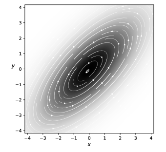
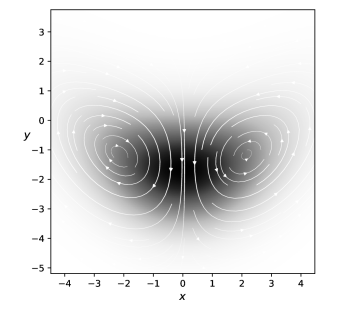
Figure 1: Nonequilibrium steady-states. Prototypical examples of NESS, where arrows represent probability currents $p^{*}\bm{\nu}^{*}$ and the background color the density $p^{*}$. (Left panel) Basic signal-response model given by the force field $\bm{F}=[-\beta x,\gamma(x-y)]$, with $\beta=1$, $\gamma=3$, and $T=5$. Here currents are perpendicular to probability gradients, $\bm{\nu}^{*}\cdot\bm{\nabla}p^{*}=0$, while in general this holds only at the expectation level, $\langle\bm{\nu}^{*}\cdot\bm{\nabla}\ln p^{*}\rangle=0$. (Right panel) Nonlinear example within the class of signal-response models, $\bm{F}=[-\beta x,\,\gamma(\mu_{1}x^{2}-\mu_{2}-y)]$, with $\mu_{1}=2/15$ and $\mu_{2}=2$. More general examples in SM.

Linear regime.

Consider a smooth probability perturbation field $\phi\equiv\phi(\bm{x},t)$ around the steady state,

$$p=p^{*}(1+\phi),$$ (6)

and assume it to be small, $|\phi|<<1$, meaning a Radon–Nikodym derivative close to $1$ everywhere. Probability normalization implies $\langle\phi\rangle\equiv\int d\bm{x}\,p^{*}\phi=0$, where brackets denote expectations with respect to the steady-state distribution.

By expanding Eqs. (2)-(3) in the small perturbation limit $|\phi|\rightarrow 0$ one obtains

$$\partial_{t}\phi=T\nabla^{2}\phi-(\bm{\nu}^{*}-T\bm{\nabla}\ln p^{*})\cdot\bm{\nabla}\phi,$$ (7)

that is the perturbation field dynamics close to the steady-state. Note that $\bm{\nu}^{*}-T\bm{\nabla}\ln p^{*}$ is a vector field evaluated at steady-state and therefore constant in time.

If we could control the initial state of the perturbation field $\phi(0)$ and precisely measure its instantaneous relaxation dynamics $\partial_{t}\phi$, then Eq. (7) suggests a simple method to infer NESS currents $p^{*}\bm{\nu}^{*}$. Indeed, taking a set of $d$ perturbations $(\phi_{i})_{i=1,...,d}$ with linearly independent gradients $(\bm{\nabla}\phi_{i}(\bm{x}))_{i=1,...,d}$ in a point $\bm{x}$ makes Eq. (7) into an algebraic system to determine the $d$ components of $\bm{\nu}^{*}(\bm{x})$. If the same set of just $d$ perturbations has linearly independent gradients for almost every point $\bm{x}\in\mathbb{R}^{d}$, then it is sufficient to reconstruct the full NESS mean local velocity field $\bm{\nu}^{*}$ and determine the corresponding entropy production $\sigma^{*}$.

Stability.

Consider the Kullback-Leibler divergence [27] from the steady-state $D\equiv D[\phi]$ as a coarse-grained measure of the perturbation field,

$$D\equiv\int d\bm{x}\,p\ln({p}/{p^{*}})=\frac{1}{2}\left\langle\phi^{2}\right\rangle,$$ (8)

where the last expression is valid to leading perturbation order. The time evolution of the divergence $d_{t}D\equiv dD/dt$ is calculated as

$$d_{t}D=\left\langle\phi\partial_{t}\phi\right\rangle=-T\left\langle||\bm{\nabla}\phi||^{2}\right\rangle\leq 0,$$ (9)

where integration by parts was performed assuming $p^{*}\phi\bm{\nabla}\phi$ and $p^{*}\phi^{2}\bm{\nu}^{*}$ decay fast enough at infinity. We see that $d_{t}D$ is nonpositive, and from the normalization $\langle\phi\rangle=0$ is clear that it attains zero only when $\phi=0$ everywhere, which ensures the stability of the nonequilibrium steady-state for small perturbations. In other words, Eq. (9) means that for the dynamics and assumptions made the Glansdorff-Prigogine criterion for stability is satisfied [28, 29, 30]. Note that $d_{t}D$ is independent of the NESS currents $\bm{\nu}^{*}$.

Nonequilibrium relaxation.

The analysis on the shorter timescales is continued by considering the second time derivative of the divergence, which is calculated as

$$d_{t}^{2}D=2T\left\langle\alpha^{2}T-\alpha\bm{\nu}^{*}\cdot\bm{\nabla}\phi\right\rangle,$$ (10)

where $\alpha\equiv\bm{\nabla}\ln p^{*}\cdot\bm{\nabla}\phi+\nabla^{2}\phi$ is an integrand independent of the NESS currents $\bm{\nu}^{*}$. Let us denote by $D^{eq}$ the divergence of the corresponding equilibrium dynamics obtained from Eq. (4) and starting from the same initial perturbation $\phi(0)$. The nonequilibrium impact on the second derivative is then written

$$\xi\equiv d_{t}^{2}D-d_{t}^{2}D^{eq}=-2T\left\langle\alpha\bm{\nu}^{*}\cdot\bm{\nabla}\phi\right\rangle,$$ (11)

which is an integral relation connecting the relaxation dynamics on short timescales to the probability currents at steady-state through their projections on perturbation gradients, and it is the first main result of this Letter.

Taking the square of Eq. (11), applying the absolute value majorization and the Cauchy-Schwarz inequality first to the dot product and then to the integral, a lower bound on the steady-state entropy production is derived,

$$\sigma^{*}\geq\frac{\xi^{2}}{4T^{3}\left\langle\alpha^{2}||\bm{\nabla}\phi||^{2}\right\rangle},$$ (12)

valid for relaxation dynamics from small perturbation fields. The squared nonequilibrium correction to the second derivative $\xi^{2}$ is a property of relaxation on short timescales, and the integral $\left\langle\alpha^{2}||\bm{\nabla}\phi||^{2}\right\rangle$ is a property of the applied initial perturbation field.

Random fields with weak spatial gradients in 2D.

In the following, starting back from the integral relation of Eq. (11), a particular ensemble of random perturbation fields is considered for its analytical tractability, and a simpler thermodynamic bound is derived.

Let us consider periodic perturbation fields of the form

$$\phi(0)=\epsilon\sin(\bm{k}\cdot\bm{x}+\varphi)+\eta,$$ (13)

where $\eta\equiv\eta(\epsilon,\bm{k},\varphi)$ ensures probability normalization, $\langle\phi\rangle=0$. The wave vector is written $\bm{k}=k\bm{e^{i\theta}}$, where $\bm{e^{i\theta}}=(\cos(\theta),\sin(\theta))$ is the direction unit vector in two dimensions, and $k>0$ is the spatial frequency. Note that this functional form is imposed for the initial state $\phi(t=0)$, while the dynamics could modify it for $t>0$. Please also note that the linear regime required above for deriving Eq. (11) here translates to having a small perturbation strength $\epsilon\ll 1$.

To leading order in $k$, meaning for spatially slowly varying perturbation fields where statistically $k\ll||\bm{\nabla}\ln p^{*}||$, the nonequilibrium relaxation correction of Eq. (11) becomes

$$\xi=-2T\epsilon^{2}k^{2}\cos^{2}(\varphi)\left\langle(\bm{e^{i\theta}}\cdot\bm{\nu}^{*})(\bm{e^{i\theta}}\cdot\bm{\nabla}\ln p^{*})\right\rangle,$$ (14)

so that the phase $\varphi$ effectively controls the gradient strength in the relevant region where the density is distributed.

Let us consider many replicas of the relaxation experiment with fixed perturbation strength $\epsilon$ and spatial frequency $k$, but each time with different phase $\varphi$ and direction $\theta$. Assuming both angles to be uniformly distributed one obtains $\mathbb{E}\xi=0$, where integration by parts was performed assuming that $p^{*}(\ln p^{*})\bm{\nu}^{*}$ decays fast enough at infinity.

To highlight the nonequilibrium impact on relaxation consider the variance of the correction, $\mathrm{Var}\left[\xi\right]\equiv\mathbb{E}\xi^{2}-(\mathbb{E}\xi)^{2}$, which is calculated to leading order in $k$ as

$$\mathrm{Var}(\xi)=\frac{3}{16}T^{2}\epsilon^{4}k^{4}\int\int d\bm{x}d\bm{y}\left[(\bm{\nu}^{*}_{\bm{x}}\cdot\bm{\nu}^{*}_{\bm{y}})(\bm{\nabla}p^{*}_{\bm{x}}\cdot\bm{\nabla}p^{*}_{\bm{y}})+(\bm{\nu}^{*}_{\bm{x}}\cdot\bm{\nabla}p^{*}_{\bm{y}})(\bm{\nabla}p^{*}_{\bm{x}}\cdot\bm{\nu}^{*}_{\bm{y}})\right],$$ (15)

where the below trigonometric integral was used,

$$\frac{4}{\pi}\int_{0}^{2\pi}d\theta\,(\mathbf{a}\cdot\bm{e^{i\theta}})(\mathbf{b}\cdot\bm{e^{i\theta}})(\mathbf{c}\cdot\bm{e^{i\theta}})(\mathbf{d}\cdot\bm{e^{i\theta}})\\ =(\mathbf{a}\cdot\mathbf{b})(\mathbf{c}\cdot\mathbf{d})+(\mathbf{a}\cdot\mathbf{c})(\mathbf{b}\cdot\mathbf{d})+(\mathbf{a}\cdot\mathbf{d})(\mathbf{c}\cdot\mathbf{b}),$$ (16)

and one can now appreciate that the simple periodic form of the perturbation field chosen in Eq. (13) was useful for the analytical evaluation of spatial correlations. Higher order terms neglected in Eqs. (14)-(15) are listed in the Supplementary Materials (SM), as well as an alternative expression for $\mathrm{Var}(\xi)$.

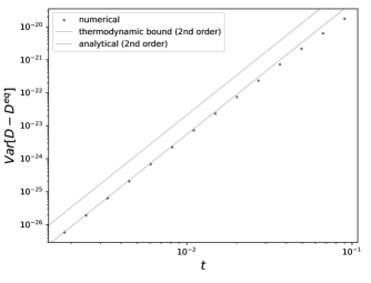
Figure 2: Linear example. Variance of the nonequilibrium impact on relaxation in the basic signal-response model with $\beta=1$, $\gamma=3$, $T=5$, and perturbations parameters $\epsilon=0.01$ and $k=0.01$.

Thermodynamic bound.

Let us define the spatial Fisher information [27] as

$$J\equiv T^{2}\left\langle||\bm{\nabla}\ln p^{*}||^{2}\right\rangle\geq 0,$$ (17)

and note that it is a property of the steady-state independent of currents. Physically it is the average squared equilibrium force $J=\left\langle||\bm{F}^{eq}||^{2}\right\rangle$ needed to produce the corresponding equilibrium steady-state.

From Eq. (15), applying the absolute value majorization and the Cauchy-Schwarz inequality first to the dot products and then to the resulting squared integral, one obtains

$$\sigma^{*}\geq\frac{8}{3}\frac{\mathrm{Var}(\xi)}{T\epsilon^{4}k^{4}J},$$ (18)

that is a refinement of the second law of thermodynamics for the NESS entropy production based on properties of relaxation on the shorter timescales, and it is the second main result of this Letter. The idea is that $\epsilon^{4}k^{4}$ is a controllable property of the ensemble of perturbations, while the spatial Fisher information $J$ can precisely be estimated from the steady-state density.

The motivation for introducing expectations instead of optimizing the lower bound of Eq. (12) over the replicas is that in the presence of measurement noise the estimation of a maximum is a statistically more involved problem. Please also note that by applying the random fields expectations directly on Eq. (12) one would get a less tight inequality than Eq. (18), consistent with the fact that majorization and expectation do not commute.

Measuring $\xi$.

The applicability of Eq. (18) for the estimation of the NESS entropy production is based on the measurement of the nonequilibrium relaxation correction $\xi$. While it is assumed that the relaxation dynamics of the nonequilibrium system under study is observable at least at the coarse-grained level of the divergence $d_{t}^{2}D$, the corresponding equilibrium dynamics $d_{t}^{2}D^{eq}$ has to be predicted from the steady-state density $p^{*}$. For the periodic perturbation fields with weak gradient considered here, this is calculated to leading order in $k$ as

$$d_{t}^{2}D^{eq}=2T^{2}\epsilon^{2}k^{2}\cos^{2}(\varphi)\left\langle(\bm{e^{i\theta}}\cdot\bm{\nabla}\ln p^{*})^{2}\right\rangle.$$ (19)

Basic linear signal-response model.

As a first example application, let us consider the stochastic dynamics of two variables $(x,y)$ where $x$ influences the dynamics of $y$ without feedback. The basic linear signal-response model [31] is defined by the drift field $\bm{F}=[-\beta x,\,\gamma(x-y)]$, with $\beta$ and $\gamma$ positive constants. The resulting probability currents are plotted in Fig. (1) left panel. This is possibly the simplest example in the class of non-reciprocal interactions models, whose asymmetry is known to produce entropy production [32, 33, 34].

Numerical verification of the results of Eqs. (15)-(18) are shown in Fig. (2), where the points falling below the $t^{2}$ line are expected as both the equilibrium and nonequilibrium dynamics relax to the same steady-state, meaning $D-D^{eq}\rightarrow 0$ for $t\rightarrow\infty$ for any small perturbation.

Analytical expressions for all the quantities involved have been derived and reported in SM. Consider here the interesting aspect of the tightness of the thermodynamic bound, that is the ratio $q$ of the entropy production with respect to the RHS of Eq. (18). For this example this is

$$q=\frac{2(1+\delta^{2})^{2}}{4\delta^{4}+(1-\delta)^{4}}\geq 1,$$ (20)

where $\delta\equiv\gamma/(\gamma+\beta)$ has been defined, and accordingly $0\leq\delta\leq 1$. The tightness ratio $q$ has an optimum of $q=2$ reached at the borders of the $\delta$ domain, and it has been plotted in Fig. (3) for the reader’s convenience. This $q=2$ optimum and the symmetries in the integral of Eq. (15) suggest that the derivation of the thermodynamic bound could possibly be refined further.

Nonlinear examples.

A first nonlinear example is again in the class of signal-response models. This corresponds to the quadratic interaction $\bm{F}=[-\beta x,\,\gamma(\mu_{1}x^{2}-\mu_{2}-y)]$, and the resulting probability currents are plotted in Fig. (1) right panel. The analytical formula of Eq. (15) and the thermodynamic bound of Eq. (18) are numerically verified and shown in SM Fig. A1.

The theoretical predictions have also been numerically verified on a more general class of random polynomial densities beyond the signal-response examples, see SM for details.

Figure 3: How tight is the bound. The basic signal-response model enables the analytical evaluation of all quantities involved, so one can immediately study how tight the thermodynamic bound here is. The tightness $q$, where $q=1$ means saturation, reaches its optimal value $q=2$ at the two domain limits, see Eq. (20).

Discussion.

Signatures of nonequilibrium in the dynamics of relaxation were previously identified both in the master equation and in the Fokker-Planck equation for the longest timescale [18, 19, 20, 21, 22, 35]. In this Letter, the entropy production in nonequilibrium steady-states of the Fokker-Planck equation has been related instead to the dynamics of relaxation on short timescales, providing a new refinement of the second law useful when fluctuations are not experimentally accessible. The advantage of considering shorter timescales is that the dynamics is more macroscopic, while the limitation of this approach is the small perturbation regime common to linear response theory [36].

References

- Risken [1996] H. Risken, Fokker-planck equation (Springer, 1996).
- Ito [2024] S. Ito, Geometric thermodynamics for the fokker–planck equation: stochastic thermodynamic links between information geometry and optimal transport, Information Geometry 7, 441 (2024).
- Dechant et al. [2022] A. Dechant, S.-i. Sasa, and S. Ito, Geometric decomposition of entropy production in out-of-equilibrium systems, Physical Review Research 4, L012034 (2022).
- Pigolotti et al. [2017] S. Pigolotti, I. Neri, É. Roldán, and F. Jülicher, Generic properties of stochastic entropy production, Physical review letters 119, 140604 (2017).
- Van den Broeck and Esposito [2010] C. Van den Broeck and M. Esposito, Three faces of the second law. ii. fokker-planck formulation, Physical Review E 82, 011144 (2010).
- Jarzynski [2011] C. Jarzynski, Equalities and inequalities: Irreversibility and the second law of thermodynamics at the nanoscale, Annu. Rev. Condens. Matter Phys. 2, 329 (2011).
- Sagawa and Ueda [2012] T. Sagawa and M. Ueda, Nonequilibrium thermodynamics of feedback control, Physical Review E 85, 021104 (2012).
- Parrondo et al. [2015] J. M. Parrondo, J. M. Horowitz, and T. Sagawa, Thermodynamics of information, Nature physics 11, 131 (2015).
- Seifert [2019] U. Seifert, From stochastic thermodynamics to thermodynamic inference, Annual Review of Condensed Matter Physics 10, 171 (2019).
- Barato and Seifert [2015] A. C. Barato and U. Seifert, Thermodynamic uncertainty relation for biomolecular processes, Physical review letters 114, 158101 (2015).
- Dechant and Sasa [2018] A. Dechant and S.-i. Sasa, Current fluctuations and transport efficiency for general langevin systems, Journal of Statistical Mechanics: Theory and Experiment 2018, 063209 (2018).
- Horowitz and Gingrich [2020] J. M. Horowitz and T. R. Gingrich, Thermodynamic uncertainty relations constrain non-equilibrium fluctuations, Nature Physics 16, 15 (2020).
- Falasco et al. [2020] G. Falasco, M. Esposito, and J.-C. Delvenne, Unifying thermodynamic uncertainty relations, New Journal of Physics 22, 053046 (2020).
- Falasco and Esposito [2020] G. Falasco and M. Esposito, Dissipation-time uncertainty relation, Physical Review Letters 125, 120604 (2020).
- Lucente et al. [2022] D. Lucente, A. Baldassarri, A. Puglisi, A. Vulpiani, and M. Viale, Inference of time irreversibility from incomplete information: Linear systems and its pitfalls, Physical Review Research 4, 043103 (2022).
- Dieball and Godec [2023] C. Dieball and A. Godec, Direct route to thermodynamic uncertainty relations and their saturation, Physical Review Letters 130, 087101 (2023).
- Freitas and Esposito [2022] J. N. Freitas and M. Esposito, Emergent second law for non-equilibrium steady states, Nature Communications 13, 5084 (2022).
- Coghi et al. [2021] F. Coghi, R. Chetrite, and H. Touchette, Role of current fluctuations in nonreversible samplers, Physical Review E 103, 062142 (2021).
- Duncan et al. [2017] A. B. Duncan, N. Nüsken, and G. A. Pavliotis, Using perturbed underdamped langevin dynamics to efficiently sample from probability distributions, Journal of Statistical Physics 169, 1098 (2017).
- Rey-Bellet and Spiliopoulos [2015] L. Rey-Bellet and K. Spiliopoulos, Irreversible langevin samplers and variance reduction: a large deviations approach, Nonlinearity 28, 2081 (2015).
- Bao and Hou [2023] R. Bao and Z. Hou, Universal trade-off between irreversibility and relaxation timescale, arXiv e-prints , arXiv (2023).
- Kolchinsky et al. [2024] A. Kolchinsky, N. Ohga, and S. Ito, Thermodynamic bound on spectral perturbations, with applications to oscillations and relaxation dynamics, Physical Review Research 6, 013082 (2024).
- Karatzas and Shreve [2012] I. Karatzas and S. Shreve, Brownian motion and stochastic calculus, Vol. 113 (Springer Science & Business Media, 2012).
- Hatano and Sasa [2001] T. Hatano and S.-i. Sasa, Steady-state thermodynamics of langevin systems, Physical review letters 86, 3463 (2001).
- Dechant and Sasa [2020] A. Dechant and S.-i. Sasa, Fluctuation–response inequality out of equilibrium, Proceedings of the National Academy of Sciences 117, 6430 (2020).
- Dechant and Sasa [2021] A. Dechant and S.-i. Sasa, Continuous time reversal and equality in the thermodynamic uncertainty relation, Physical Review Research 3, L042012 (2021).
- Dembo et al. [1991] A. Dembo, T. M. Cover, and J. A. Thomas, Information theoretic inequalities, IEEE Transactions on Information theory 37, 1501 (1991).
- Ito [2022] S. Ito, Information geometry, trade-off relations, and generalized glansdorff–prigogine criterion for stability, Journal of Physics A: Mathematical and Theoretical 55, 054001 (2022).
- Maes and Netočnỳ [2015] C. Maes and K. Netočnỳ, Revisiting the glansdorff–prigogine criterion for stability within irreversible thermodynamics, Journal of Statistical Physics 159, 1286 (2015).
- Glansdorff et al. [1974] P. Glansdorff, G. Nicolis, and I. Prigogine, The thermodynamic stability theory of non-equilibrium states, Proceedings of the National Academy of Sciences 71, 197 (1974).
- Auconi et al. [2017] A. Auconi, A. Giansanti, and E. Klipp, Causal influence in linear langevin networks without feedback, Physical Review E 95, 042315 (2017).
- Auconi et al. [2019] A. Auconi, A. Giansanti, and E. Klipp, Information thermodynamics for time series of signal-response models, Entropy 21, 177 (2019).
- Loos and Klapp [2020] S. A. Loos and S. H. Klapp, Irreversibility, heat and information flows induced by non-reciprocal interactions, New Journal of Physics 22, 123051 (2020).
- Zhang et al. [2023] Z. Zhang, R. Garcia-Millan, et al., Entropy production of nonreciprocal interactions, Physical Review Research 5, L022033 (2023).
- Dechant et al. [2023] A. Dechant, J. Garnier-Brun, and S.-i. Sasa, Thermodynamic bounds on correlation times, arXiv preprint arXiv:2303.13038 (2023).
- Kubo et al. [2012] R. Kubo, M. Toda, and N. Hashitsume, Statistical physics II: nonequilibrium statistical mechanics, Vol. 31 (Springer Science & Business Media, 2012).