PE: A Poincare Explanation Method for Fast Text Hierarchy Generation

Abstract

The black-box nature of deep learning models in NLP hinders their widespread application. The research focus has shifted to Hierarchical Attribution (HA) for its ability to model feature interactions. Recent works model non-contiguous combinations with a time-costly greedy search in Eculidean spaces, neglecting underlying linguistic information in feature representations. In this work, we introduce a novel method, namely Poincaré  Explanation (PE), for modeling feature interactions using hyperbolic spaces in an $O(n^{2}logn)$ time complexity. Inspired by Poincaré  model, we propose a framework to project the embeddings into hyperbolic spaces, which exhibit better inductive biases for syntax and semantic hierarchical structures. Eventually, we prove that the hierarchical clustering process in the projected space could be viewed as building a minimum spanning tree and propose a time efficient algorithm. Experimental results demonstrate the effectiveness of our approach. Our code is available at https://github.com/qq31415926/PE.

PE: A Poincare Explanation Method for Fast Text Hierarchy Generation

Qian Chen¹, Xiaofeng He^1,2 , Hongzhao Li³, Hongyu Yi^{3 1} School of Computer Science and Technology, East China Normal University, Shanghai, China ² NPPA Key Laboratory of Publishing Integration Development, ECNUP, Shanghai, China ³ Sichuan Caizi Software Information Network Co., Ltd qianchen901005@gmail.com, hexf@cs.ecnu.edu.cn, lhz@sxw.cn,alwayslater@yeah.net

1 Introduction

Deep learning models have been ubiquitous in Natural Language Processing (NLP) areas accompanied by the explosion of the parameters, leading to increased opaqueness. Consequently, a series of interpretability studies have emerged Abnar and Zuidema (2020); Geva et al. (2021); He et al. (2022), among them feature attribution methods stand out owing to fidelity and loyalty axioms and straightforward applicability Guidotti et al. (2018).

Previous feature-based works are limited to single words or phrases Ribeiro et al. (2016). However, as shown in Figure 3, Mardaoui and Garreau (2021) point out that LIME’s performance on simple models is not plausible. To mitigate this, Hierarchical Attribution (HA) has been introduced, which constructs a complete process of feature interaction by calculating the text groups at different levels, as shown in Figure 1. From bottom to the up, hierarchical attribution categorizes all words into different clusters, ending with a tree structure.

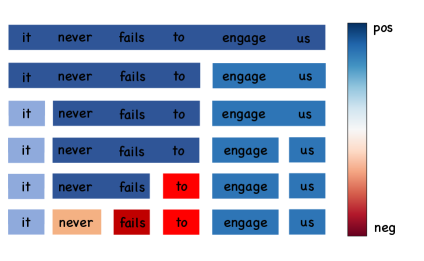
Figure 1: A hierarchy example from HEDGE Chen et al. (2020). The background color of the words and phrases represents emotional polarity, with cool colors indicating positive and warm colors indicating negative.

However, existing methods modeling non-contiguous feature combinations require exhaustive enumerations of possible word combinations, as shown in Table 1. Only using spans might lose long-range dependencies in text Vaswani et al. (2017). For example, in the positive example “Even in moments of sorrow, certain memories can evoke happiness”, “Even, sorrow” is vital and non-adjacent. Current methods estimate the importance of feature combinations using algorithms like LIME or Shapley value. For example, HE Ju et al. (2023) estimates the importance of words using LIME algorithm and then enumerates word combinations to solve the hierarchy, with a time complexity of $O(n^{3})$. ASIV Lu et al. (2023) uses directional Shapley value to model the direction of feature interactions, while estimating Shapley value is time-consuming.

Linguistic information such as syntax and semantics can help to construct a hierarchical tree. Text inherently possesses a hierarchical prior and hyperbolic space is more powerful than Euclidean space in modeling hierarchies Ganea et al. (2018). In previous studies, discussions often focuses on the influence of feature interactions on output probability, neglecting the auxiliary information provided by semantics and syntax, which can assist in producing more comprehensible results. As shown in Figure 2, the hierarchy in hyperbolic space has already achieved preliminary interpretability.

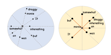
Figure 2: A projection example for sentence “It was an interesting but somewhat draggy movie.” Left panel: The circle with a blue background represents the projected space related to semantics, with the central point representing the prototype for the positive label. Right panel: The circle with a goose-yellow background represents the projected space related to syntax, with proximity to the center indicating the level it is in the dependency tree.

As the number of parameters in NLP models continues to increase, efficiently modeling the interaction of non-contiguous features has become a key challenge in promoting HA.

Method	Non-Contiguous	Time Complexity
ACD (2019)	Not available	$O(n^{2}logn)$
HEDGE (2020)	Not available	$O(n^{3})$
HE (2023)	Available	$O(n^{3})$
PE (ours)	Available	$O(n^{2}logn)$

Table 1: Comparison results of HA methods about capturing non-contiguous interactions and their time complexity of building hierarchical trees. $n$ is the sequence length.

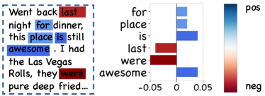
Figure 3: A LIME explanation example from a random forest classifier. It can be observed that ‘is’ and ‘were’ are identified as positive and negative emotional polarities, respectively.

Building a hierarchical attribution tree based on the input text is essentially a hierarchical clustering problem. The definition is as follows: given words and their pairwise similarities, the goal is to construct a hierarchy over clusters. PE approaches this problem by following three steps. First, to undermine linguistic hierarchical information, we project word embeddings into hyperbolic spaces, then we calculate pairwise similarities. Next, inspired by cooperative game theory Owen (2013), we regard words as players and clusters as coalitions, then introduce a simple yet effective strategy to estimate the contribution. Finally inspired by Dasgupta (2016), we propose an algorithm that conceptualizes the bottom-up clustering process as a super additivity game, ensuring the optimal payoff of each merge, thereby analogizing the entire process as generating a minimum spanning tree.

Our contributions are summarized as follows:

• We propose a method using hyperbolic geometry for generating hierarchical explanations, revealing the feature interaction process.

• We propose a fast algorithm for generating hierarchical attribution trees that model non-contiguous feature interactions.

• We evaluate the proposed method on three classification datasets with BERT Devlin et al. (2019), and the results demonstrate the effectiveness .

2 Related Work

Feature importance explanation methods mainly assign attribution scores to features Qiang et al. (2022); Ferrando et al. (2022); Modarressi et al. (2023). Methods can be classified into two categories: single-feature explanation type and multi-feature explanation type.

2.1 Single-Feature Explanation

Earlier researches focus on single feature attribution Ribeiro et al. (2016); Sundararajan et al. (2017); Kokalj et al. (2021). For example, LIME Ribeiro et al. (2016) aims to fit the local area of the model by linear regression with sampled data points ending with linear weights as attribution scores. Gradient*Input (Grad*Inp) Shrikumar et al. (2017b) combines the gradient norm with Shapley value Shapley et al. (1953). Deeplift Shrikumar et al. (2017a) depends on activation difference to calculate attribution scores. IG Sundararajan et al. (2017); Sanyal and Ren (2021); Enguehard (2023); Chen et al. (2023) uses path integral to compute the contribution of the single feature to the output. It is noticeable that IG is the unique path method to satisfy the completeness and symmetry-preserving axioms. There exist several variants of IG. DIG Sanyal and Ren (2021) regards similar words as interpolation points to estimate the integrated gradients value. SIG Enguehard (2023) computes the importance of each word in a sentence while keeping all other words fixed.

2.2 Multi-Feature Explanation

Multi-feature explanation methods aim to model feature interactions in deep learning architectures. For example, Dhamdhere et al. (2020) proposes a variant of Shapley value to measure the interactions. Zhang et al. (2021a) defines the multivariant Shapley value to analyze interactions between two sets of players. Enouen and Liu (2022) proposes a sparse interaction additive network to select feature groups. Tsang et al. (2020) proposes an Archipelago framework to measure feature attribution and interaction through ArchAttribute and ArchDetect. Lu et al. (2023) proposes ASIV to model asymmetric higher-order feature interactions.

Additionally, the explanation of feature interaction could be articulated within a hierarchical framework. HEDEG Chen et al. (2020) designs a top-down model-agnostic hierarchical explanation method. Ju et al. (2023) addresses the connecting rule limitation in HEDGE, and proposes a greedy algorithm for generating hierarchical explanations.

3 Background

We first give a review of hyperbolic geometry.

Poincaré ball A common representation model in hyperbolic space is the Poincaré ball, denoted as $(\mathcal{B}_{c}^{n},g_{\boldsymbol{x}}^{\mathcal{B}})$, where $c$ is a constant greater than $0$. $\mathcal{B}_{c}^{n}=\{\boldsymbol{x}\in\mathbb{R}^{n}\mid c\left\|\boldsymbol{x}\right\|^{2}<1\}$ is a Riemannian manifold, and $g_{\boldsymbol{x}}^{\mathcal{B}}=(\lambda_{\boldsymbol{x}}^{c})^{2}\boldsymbol{I}_{n}$ is its metric tensor, $\lambda_{\boldsymbol{x}}^{c}=2/(1-c\left\|\boldsymbol{x}\right\|^{2})$ is the conformal factor and $c$ is the negative curvature of the hyperbolic space. The distance for $\boldsymbol{x},\boldsymbol{y}\in\mathcal{B}_{c}^{n}$ is:

$$d_{\mathcal{B}}(\boldsymbol{x},\boldsymbol{y})=(2/\sqrt{c})\tanh^{-1}{\sqrt{c}\left\|-\boldsymbol{x}\oplus_{c}\boldsymbol{y}\right\|},$$ (1)

where $\oplus_{c}$ denotes the Möbius addition. We use $\otimes_{c}$ to denote the Möbius matrix multiplication.

4 Methodology

This section mainly provides a detailed introduction to the three parts of PE. We use following notations. For a classification task, given a sequence $X_{i}=\{x_{j}\}_{1\leq j\leq n}$ and a trained model $f$, $n$ is the sequence length. $\hat{y}$ represents the predicted label, and $f(\cdot)$ represents the model’s output probability for the predicted label.

4.1 Poincaré Projection

In this paper, we choose Probing Hewitt and Manning (2019) to recover information from embeddings.

4.1.1 Label Aware Probing

First, we feed the sequence $X_{i}$ into BERT to obtain the contextualized representations $\boldsymbol{E}_{i}\in\mathbb{R}^{n\times d_{in}}$. Next, the sentence embedding $\boldsymbol{s}_{i}\in\mathbb{R}^{d_{in}}$ is calculated by the hidden representations of the [CLS] tag, which is the first token of the sequence and used for classification tasks. Our probing matrix consists of two types: $\boldsymbol{P}_{c},\boldsymbol{P}_{s}\in\mathbb{R}^{d_{in}\times d_{out}}$ for probing label-aware semantic information and probing syntax information. For semantics, we can obtain the projected representation:

$$\boldsymbol{s}_{c,i}=\boldsymbol{P}_{c}\otimes_{c}\boldsymbol{s}_{i}.$$ (2)

To train the probing matrices, we draw inspiration from prototype networks Snell et al. (2017), assuming that there exist $k$ centroids representing labels in the hyperbolic space. The closer a point is to a centroid, the higher the probability that it belongs to that category. Specifically, instead of using mean pooling to calculate the prototypes, we directly initialize the prototype embeddings in hyperbolic space, denoted as $\boldsymbol{\phi}=\{\boldsymbol{c}_{k}\}$. Given a distance $d_{\mathcal{B}}$, the prototypes produce a distribution over classes for a point $\boldsymbol{x}$ based on a softmax over distances to prototypes in the embedding space:

$$\mathcal{P}(y=k\mid\boldsymbol{\phi})=\frac{exp(-d_{\mathcal{B}}(\boldsymbol{s}_{c,i},\boldsymbol{c}_{k}))}{\sum_{k^{\prime}}{exp(-d_{\mathcal{B}}(\boldsymbol{s}_{c,i},\boldsymbol{c}_{k^{\prime}}))}}.$$ (3)

We minimize the negative log-probability $J(\boldsymbol{\phi})=-log\mathcal{P}(y=k\mid\boldsymbol{\phi})$ of the true class $k$ via RiemannianAdam Kochurov et al. (2017).

4.1.2 Syntax Probing

We project word embeddings first:

$$\boldsymbol{h}_{s,j}=\boldsymbol{P}_{s}\otimes_{c}\boldsymbol{e}_{j},$$ (4)

where $\boldsymbol{e}_{j}=\boldsymbol{E}_{j,:}$. How to parameterize a dependency tree from dense embeddings is non-trivial. Following the idea of Hewitt and Manning (2019), we define two metrics to measure the deviation from the standard: using the distance between two words in embedding space to represent the distance of word nodes in the dependency tree, and using the distance of a word from the origin to represent the depth of the word node. And similar to Hewitt and Manning (2019), we use the following two loss functions:

$$\mathcal{L}_{\text{dist}}=\frac{1}{n^{2}}\sum\limits_{j,k\in[n]}{|d_{T}(w_{j},w_{k})-d_{\mathcal{B}}(\boldsymbol{h}_{s,j},\boldsymbol{h}_{s,k})^{2}|},$$ (5)

$$\mathcal{L}_{\text{dep}}=\frac{1}{n}\sum\limits_{j\in[n]}{|d_{D}(w_{j})-d_{\mathcal{B}}(\boldsymbol{h}_{s,j},\boldsymbol{0})^{2}|}.$$ (6)

where $d_{T}(w_{j},w_{k})$ and $d_{D}(w_{j})$ represent the distance of words and the depth of words respectively.

4.2 Feature Contribution Estimation

According to cooperative game theory, we regard the input as a set of players $N$, where each element of the set corresponds to a word, and the process of hierarchical clustering is viewed as a super additivity game, with clusters containing more than two words considered a coalition. Following Zhang et al. (2021b), we define the characteristic function as $v=f$. Given a game $\Gamma=(N,v)$, a fair payment scheme rewards each player according to his contribution. The Shapley value removes the dependence on ordering by taking the average over all possible orderings for fairness. The Shapley value of player $i$ in a game is as follows:

$$\phi_{i}=\frac{1}{|N|!}\sum\limits_{\pi\in\Pi(N)}[v(P_{i}^{\pi}\cup\{i\})-v(P_{i}^{\pi})],$$ (7)

where $\Pi(N)$ is the set of all permutations of the players, $P_{i}^{\pi}$ is the set of players preceding player $i$ in permutation $\pi$. $v(S)$ is the value that the coalition of players $S\subseteq N$ can achieve together. In practical , we use Monte Carlo sampling to compute:

$$\hat{\phi_{i}}=\frac{1}{M}\sum\limits_{m=1}^{M}{v(P_{i}^{\pi(m)}\cup\{i\})-v(P_{i}^{\pi(m)})}.$$ (8)

Unfortunately, Monte Carlo sampling methods can exhibit slow convergence Mitchell et al. (2022). It is noticeable that attention mechanism of Transformer is permutation invariant Vaswani et al. (2017); Xilong et al. (2023), and the sinusoidal position embedding is only related to the specific position, not to the word. Moreover, after being trained with a Masked Language Model task, the model has the ability to fill in the blanks based on context Devlin et al. (2019). Therefore, we assume that it is unnecessary to enumerate exponential combinations of words. In this work, we directly calculate contributions as follows:

$$\tilde{\phi}_{i}=v(N_{i}\cup\{i\})-v(N_{i})$$ (9)

4.3 Minimum Spanning Tree

Our goal is to identify a binary tree that aligns with semantic similarities, syntax similarities, and the contributions of individual elements. Building upon Dasgupta (2016), we use the following cost:

$$C_{D}(T;e)=\sum_{i,j\in[n]}e_{ij}|leaves(T[i\vee j])|,$$ (10)

where $e_{i,j}$ denotes the pairwise similarities, $leaves(T[i\vee j])$ is leaves of $T[i\vee j]$, which is the subtree rooted at $[i\vee j]$, as shown in Figure 4. Due to the unfolding dilemma of $leaves(T[i\vee j])$ process, we adopt following expansion by Wang and Wang (2018):

$$\begin{split}C_{D}(T;e)&=\sum\limits_{ijk\in[n]}[e_{ij}+e_{ik}+e_{jk}\\ &\quad-e_{ijk}(T;w)]+2\sum\limits_{ij}e_{ij},\end{split}$$ (11)

where

$$\begin{split}e_{ijk}(T;w)=&e_{ij}\mathbbm{1}[\{i,j\mid k\}]+e_{ik}\mathbbm{1}[\{i,k\mid j\}]\\ &\quad+e_{jk}\mathbbm{1}[\{j,k\mid i\}],\end{split}$$ (12)

where $\{i,j\mid k\}$ denotes the $i\vee j$ is the descendant of $i\vee j\vee k$, illustrated in Figure 4. The same for $\{i,k\mid j\}$ and $\{j,k\mid i\}$.

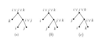
Figure 4: Three different binary tree types rooted from $i\vee j\vee k$.

Directly optimizing this cost presents a combinatorial optimization problem. We introduce the following decomposition assumption:

$$\begin{split}e_{ij}=&-\tilde{\phi}(i\vee j)+\alpha_{1}d_{\mathcal{B}}(\boldsymbol{h}_{c,i},\boldsymbol{h}_{c,j})\\ &+\frac{1}{2}\alpha_{2}(d_{\mathcal{B}}(\boldsymbol{h}_{s,i},\boldsymbol{0})+d_{\mathcal{B}}(\boldsymbol{h}_{s,j},\boldsymbol{0})),\end{split}$$ (13)

where $\boldsymbol{h}_{c,i}=\boldsymbol{P}_{c}\otimes_{c}\boldsymbol{E}_{i,:}$, $\alpha_{1}\text{,}\alpha_{2}\in[0,1]$. Our goal is to find the binary tree $T^{*}$:

$$T^{*}=\mathop{\text{argmin}}_{\text{all binary trees }T}C_{D}(T;e).$$ (14)

We introduce the following decoding algorithm and prove that under the decomposition assumption, the optimal tree $T^{*}$ is a like-minimum spanning tree of 11. The proof is available in Appendix A.

Algorithm 1 Decoding Algorithm

0:  Label hyperbolic embeddings $\boldsymbol{H}_{1}=\{\boldsymbol{h}_{c,1},\cdots,\boldsymbol{h}_{c,n}\}$, syntax hyperbolic embeddings $\boldsymbol{H}_{2}=\{\boldsymbol{h}_{s,1},\cdots,\boldsymbol{h}_{s,n}\}$

0:  Binary tree $T$ with $n$ leafs

1:  $T\leftarrow(\{i\}:i\in N)$

2:  Initialize a PriorityQueue $Q$

3:  $Q\leftarrow\{(i,j):\text{pairs sorted by}\,e_{ij}\}$

4:  while $Q\neq\varnothing$ do

5:     $i,j\leftarrow Q.$front, $Q.$pop

6:     if $i$ and $j$ not in $T$ then

7:        $T\leftarrow T\cup\{i\vee j\}$

8:        $Q.$push($i\vee j$)

9:     end if

10:  end while

5 Experiments

5.1 Experimental Setups

Datasets and Models To evaluate the effectiveness of PE, we perform comprehensive experiments on three representative text classification datasets: “Rotten Tomatoes” Pang and Lee (2005), “TREC” Li and Roth (2002), “Yelp” Zhang et al. (2015). Detailed statistics are in Table 2.

Dataset	Train/Dev/Test	C	L
Rotten Tomatoes	10K/2K/2K	2	64
TREC	5000/452/500	6	64
Yelp	10K/2K/1K	2	256

Table 2: Statistics of three datasets. C: number of classes, L: average text length

Metrics Following prior literature DeYoung et al. (2020), we use AOPC metric, which is the average difference of the change in predicted class probability before and after removing top $K$ words.

$$\text{AOPC}=\frac{1}{n}\sum_{K}(f(x_{i})-f(\tilde{x}_{i}^{K}))$$ (15)

Higher is better. And we evaluate two different strategies: $del$ and $pad$. Concretely, We assign values to words through the following formula:

$$\text{score}_{i}=\tilde{\phi}(i)-\beta_{1}d_{\mathcal{B}}(\boldsymbol{h}_{c,i},\boldsymbol{c}_{k})-\beta_{2}d_{\mathcal{B}}(\boldsymbol{h}_{s,i},\boldsymbol{0}),$$ (16)

where $\boldsymbol{c}_{k}$ is the prototype of predicted label $k$ in the semantic hyperbolic space, $\boldsymbol{0}$ is the origin in the syntatic hyperbolic space, $\beta_{1},\beta_{2}\in[0,1]$.

Baselines We compare other methods against four hierarchical attribution methods: SOC Jin et al. (2020), HEDGE Chen et al. (2020), $\text{HE}_{LIME}$ , $\text{HE}_{LOO}$ Ju et al. (2023) and two feature interaction methods: Bivariate Shapley value Masoomi et al. (2022) and ASIV Lu et al. (2023).

Methods/ Datasets	Rotten Tomatoes				TREC
	$\text{AOPC}_{del}$		$\text{AOPC}_{pad}$		$\text{AOPC}_{del}$		$\text{AOPC}_{pad}$
	$10\%$	$20\%$	$10\%$	$20\%$	$10\%$	$20\%$	$10\%$	$20\%$
SOC Jin et al. (2020)	0.102	0.117	0.149	0.153	0.074	0.087	0.097	0.099
HEDGE Chen et al. (2020)	0.087	0.134	0.084	0.194	0.068	0.079	0.095	0.101
$\text{HE}_{LIME}$ Ju et al. (2023)	0.075	0.195	0.076	0.193	0.063	0.072	0.059	0.066
$\text{HE}_{LOO}$ Ju et al. (2023)	0.062	0.117	0.061	0.119	0.081	0.092	0.075	0.086
Bivariate Shapley value Masoomi et al. (2022)	0.109	0.121	0.103	0.185	0.099	0.104	0.097	0.105
ASIV Lu et al. (2023)	0.101	0.113	0.098	0.181	0.093	0.106	0.092	0.113
PE (ours)	0.304	0.352	0.364	0.313	0.214	0.220	0.183	0.174

Table 3: AOPC comparison results of PE with baselines on the Rotten Tomatoes and TREC dataset.

Datasets	Yelp
Methods	$\text{AOPC}_{del}$		$\text{AOPC}_{pad}$		$\overline{\boldsymbol{t}}$
	$10\%$	$20\%$	$10\%$	$20\%$
SOC	0.060	0.074	0.065	0.084	7.609
HEDGE	0.077	0.084	0.074	0.089	70.312
$\text{HE}_{LIME}$	0.056	0.075	0.065	0.076	20.383
$\text{HE}_{LOO}$	0.040	0.071	0.059	0.064	16.201
PE	0.110	0.138	0.112	0.143	2.230

Table 4: AOPC and time efficiency comparision results of PE and baselines on the Yelp dataset. $\overline{\boldsymbol{t}}$ denotes the average time of building HA tree, in seconds.

5.2 General Experimental Results

We first evaluate our method using the AOPC metric across three datasets, as shown in Tables 3 and 4. Firstly, our method, PE, consistently surpasses the baseline in binary and multiclass tasks for both short and long texts. For instance, PE outperforms $\text{HE}_{LOO}$ by 0.235 in Table 3 and by 0.067 in Table 4 of $\text{AOPC}_{del}$,$20\%$, Rotten Tomatoes / Yelp setting. Second, in comparison to recent works such as SOC and $\text{HE}_{LOO}$, our method’s primary advantage lies in its computation efficiency. We conduct an analysis comparing the average time of various approaches to construct HA trees. The results in Table 4 indicate that PE substantially outperforms its counterparts in terms of speed, being twice as fast as SOC and six times faster than $\text{HE}_{LIME}$.

5.3 Ablation Study

We conduct an ablation experiment with three modified baselines from PE: PE w/o prob corresponding $\tilde{\phi}(i)=0$, PE w/o semantic corresponding $\beta_{1}=0$ and PE w/o syntax corresponding $\beta_{2}=0$.

As shown in Figure 5, both PE and variants outperform w/o prob baselines, demonstrating our approach’s effectiveness in directly calculating contributions in Equation 9. Moreover, we observe that both in $del$ and $pad$ settings, the utility of estimating contribution is more striking than the other two components in Equation 16. The reason may be that context has a greater impact on output than single semantics and syntax. It is noticeable that syntax slightly outperforms semantics, we hypothesis that the reason might be related to the nature of the tasks in the TREC dataset, as the labels tend to associate with syntactic structures Li and Roth (2002).

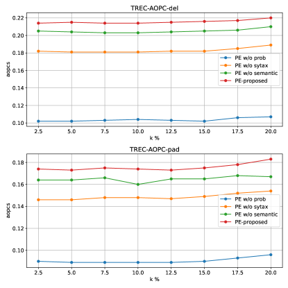
Figure 5: Evaluation results of Ablation Study.

5.4 Case Study

For qualitative analysis, we present two typical examples from the Rotten Tomatoes dataset to illustrate the role of PE in modeling the interaction of discontinuous features and we show more examples in Appendix B. In the first example, we compare the results of PE and $\text{HE}_{LOO}$ in interpreting BERT model. Figure 6 provides two hierarchical explanation examples for a positive and negative review, each generated by PE and $\text{HE}_{LOO}$ respectively. In Figure 6(a), it can be seen that PE accurately captures the combination of words with positive sentiment polarity: delightful, out, and humor, and captures the key combination of out and humor at step 1. Additionally, this example includes a word with negative polarity: stereotypes, where it can be observed that $\text{HE}_{LOO}$ captures its combination with in and delightful, missing the combination with out and humor. In Figure 6(b), PE captures the combination of slightest and wit in the first phase and complements it with the combination of lacking at step 2. HE captures the combination of combination and animation at step 1, and it adds lacking at step 2. We can infer that PE is able to capture the feature combination more related to the label at a shallow level, which demonstrates the effectiveness of our method.

Additionally, to more vividly demonstrate the role of semantics and syntax in building hierarchical explanations, we illustrate with two examples from the TREC dataset. As shown in Figure 7(a), when $\alpha_{2}=0.5$, at the level $L_{3}$, PE combines center, temperature, the, earth together. However, when $\alpha_{2}=0$, PE combines the, temperature, the, earth together. In the dependency parse tree of the sentence what is the temperature of the center of the earth, the distance to root is greater than center. This indicates that incorporating syntactic information is meaningful for constructing convincing hierarchical explanations.

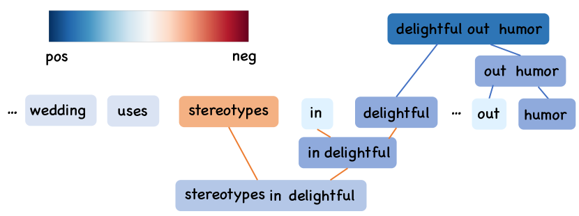
(a) A positive example “My big fat greek wedding uses stereotypes in a delightful blend of sweet romance and lovingly dished out humor.”

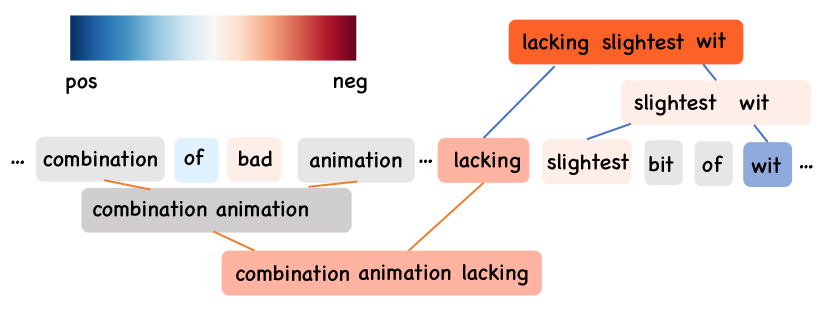
(b) A negative example “Just another combination of bad animation and mindless violence lacking the slightest bit of wit or charm.”

Figure 6: PE,$\text{HE}_{LOO}$ for BERT on two examples from the Rotten Tomatoes dataset. The subtree in the upper right corner is generated by PE and the lower is produced by $\text{HE}_{LOO}$.

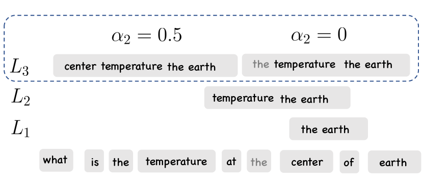
(a) An example “What is the temperature at the center of the earth?”, which the predicted label is numeric value.

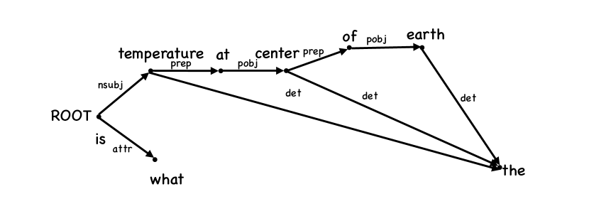
(b) A dependency parsing tree generated by Spacy Honnibal and Montani (2017).

Figure 7: PE for BERT on the example from the TREC dataset. The cluster on the left side of the third level $L_{3}$ is the results for $\alpha_{2}=0.5$, and the right side is the result for $\alpha_{2}=0$.

6 Discussion

In this section, we delve into the time complexity associated with HA methods, which can be divided into two parts: the complexity of generating attribution scores, denoted as $O_{attr}$, and the complexity of generating the hierarchy from the scores, denoted as $O_{hierarchy}$. As shown in Table 5, we elaborate on the time complexity of various methods. For score computation, HEDGE utilizes the Monte Carlo sampling algorithm, with the number of samples denoted by $m_{1}$, leading to a time complexity of $O(nm_{1})$. The SOC algorithm, defined as the expected prediction difference after masking the phrase for each replacement of contexts, also has a time complexity of $O(nm_{2})$, where $m_{2}$ denotes the number of sampling neighboring words. $\text{HE}_{LOO}$ uses the LOO algorithm Lipton (2018), with a time complexity of $O(n^{2}M)$, where $M$ is the maximum number of iterations of the LOO algorithm. $\text{HE}_{LIME}$ method employs the LIME algorithm, with ridge regression solving complexity of $O(m_{3}p^{3})$, where $m_{3}$ is the number of sampled instances and $p$ is the number of sampled features. The time complexity of PE for solving scores is $O(n^{2})$.

Method	$O_{attr}$	$O_{hierarchy}$
HEDGE (2020)	$O(nm_{1})$	$O(n^{3})$
SOC (2020)	$O(nm_{2})$	$O(n^{2}logn)$
$\text{HE}_{LOO}$ (2023)	$O(n^{2}M)$	$O(n^{3})$
$\text{HE}_{LIME}$ (2023)	$O(m_{3}p^{3})$	$O(n^{3})$
PE (ours)	$O(n^{2})$	$O(n^{2}logn)$

Table 5: Comparison results of HA methods about capturing non-contiguous interactions and their time complexity.

7 Conclusion

In this paper, we introduce PE, a computationally efficient method employing hyperbolic geometry for modeling feature interactions. More concretely, we use two hyperbolic projection matrices to embed the semantic and syntax information and devise a simple strategy to estimate the contributions of feature groups. Finally we design an algorithm to decode the hierarchical tree in an $O(n^{2}logn)$ time complexity. Based on the experimental results of three typical text classification datasets, we demonstrate the effectiveness of our method.

8 Limitations

The limitations of our work include: 1) Although our method boasts low time complexity, the use of the probing method to train additional model parameters, including two Poincare projection matrices, somewhat limits the generalizability of our approach. 2) In our experiments, we decompose the weights of the edges of the HA tree according to Equation 13. Whether there exists a more optimal decomposition formula remains a question for future investigation.

Appendix A Proof

First, we prove that the conclusion holds for $n=3$, and we generalize to the case of $n>3$ using induction.

Notation Due to the specificity of the binary tree we are solving for, a unique candidate tree can correspond to a node permutation $\pi$. For a tree with $n$ leaves, we define $\pi_{n}$ as the corresponding permutation.

We denote the constructed permutation $\pi_{n}^{*}$ and prefix permutation $\pi_{m}^{*}$ in Algorithm 1.

Base Case We here start the discussion from the left case in Figure 8. The cost can be expanded into:

$$\begin{split}C_{D}(\pi_{3}^{*};e)&=\sum\limits_{ijk}(e_{ik}+e_{jk})+2\sum\limits_{ij}e_{ij}\\ &=\sum_{ijk}2e_{ij}+e_{ik}+e_{jk}\end{split}$$ (17)

Notice that $e_{ij}$ is smallest among $e_{ij}$, $e_{ik}$, $e_{jk}$ and among $\{i,j\mid k\}$, $\{i,k\mid j\}$, $\{j,k\mid i\}$, only one will hold true. We can conclude that $\pi_{3}^{*}$ is the solution that minimizes the cost.

Induction Step We assume that the tree corresponding to the permutation $\pi_{m}$ has the smallest cost. To prove that $\pi_{m+1}$ is also the smallest. We use a proof by contradiction to demonstrate that $\pi_{m+1}$ corresponds to the tree with the smallest cost. We define the tree’s level as $L_{1},\cdots,L_{n-1}$ in Figure 8. Firstly, we introduce the following lemma:

Lemma We denote the $\gamma$-th step permutation produced in Algorithm 1 as $\pi_{\gamma}^{*}$, and its corresponding tree cost as $C(\pi_{\gamma}^{*})$. Now, if we swap the nodes at level $L_{s}$ and $L_{t}$, $s<t$, and the resulting sequence ${\pi_{\gamma}^{*}}^{\prime}$, then $C({\pi_{\gamma}^{*}}^{\prime})>C(\pi_{\gamma}^{*})$.

Proof.

We consider the cost after the swap as three parts: the triples that do not include $s$ and $t$, the part of the triples that include $s$ and the part that include $t$, denoted as $C_{1}$,$C_{2}$ and $C_{3}$. For ease of proof, we denote the sequence to the left of $s$ as $A=\pi^{*}_{\gamma,1:s-1}$, and the sequence between $s$ and $t$ as $B=\pi^{*}_{\gamma,s+1:t-1}$.

Obviously $C_{1}$ remains unchanged, as for $C_{2}$, before and after the swap:

$$C_{2}=\sum\limits_{i,j\in A,s}e(\cdot)+\sum\limits_{i\in A,s,j\in B}e(\cdot)+\sum\limits_{s,i,j\in B}e(\cdot),$$ (18)

$$C_{2}^{\prime}=\sum\limits_{i,j\in A,s}e(\cdot)+\sum\limits_{i\in A,j\in B,s}e(\cdot)+\sum\limits_{i,j\in B,s}e(\cdot)$$ (19)

By subtracting, we obtain:

$$\begin{split}C_{2}^{\prime}-C_{2}&=(\sum\limits_{i\in A,j\in B,s}e(\cdot)-\sum\limits_{i\in A,s,j\in B}e(\cdot))+\\ &(\sum\limits_{i,j\in B,s}e(\cdot)-\sum\limits_{s,i,j\in B}e(\cdot))\geq 0.\end{split}$$ (20)

Similarly we obtain:

$$\begin{split}C_{3}^{\prime}-C_{3}&=(\sum\limits_{i\in A,t,j\in B}e(\cdot)-\sum\limits_{i\in A,j\in B,t}e(\cdot))+\\ &(\sum\limits_{t,i,j\in B}e(\cdot)-\sum\limits_{i,j\in B,t}e(\cdot))\geq 0.\end{split}$$ (21)

Now we prove that $\pi_{m+1}$ is smallest. If $\pi_{m+1}$ is not the smallest, then the node at the last level can be the smallest by swapping with a previous node. There are two cases: when the swapped node is from the first level (e.g. $j$), in this case, the difference in cost before and after the swap becomes:

$$\begin{split}\Delta C&=(\sum\limits_{i\in C,m+1,j\in D}e(\cdot)-\sum\limits_{i\in C,j\in D,m+1}e(\cdot))+\\ &(\sum\limits_{t,i,j\in D}e(\cdot)-\sum\limits_{i,j\in D,t}e(\cdot))\geq 0,\end{split}$$ (22)

where $C=\pi_{m+1,1}^{*}$, $D=\pi_{m+1,3:m}^{*}$. Similarly, when the swapped node is located in other levels, the cost after the swap will not decrease. This means that in $C(\pi_{m+1})$ cannot be smaller through swapping other leaves from different levels, thus $\pi_{m+1}$ is smallest.

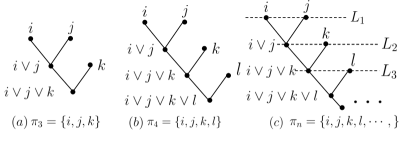
Figure 8: Examples for $\pi_{3}$, $\pi_{4}$ and $\pi_{n}$.

The primary difference is that the edge weights in our graph Graham and Hell (1985) are not all known in advance but are dynamically generated.

Appendix B Visualization

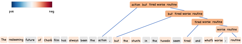
(a) A negative example “The redeeming feature of Chan’s films has always been the action, but the stunts in the tuxedo seem tired and what’s worse, routine.”

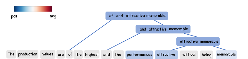
(b) A positive example “The production values are of the highest and the performances attractive without being memorable.”

Figure 9: PE for BERT on two examples from the Rotten Tomatoes dataset.

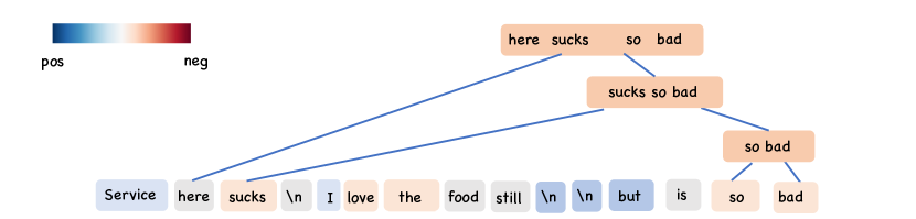
(a) A negative example “Service here sucks \n I love the food still \n\n but the service is so bad.”

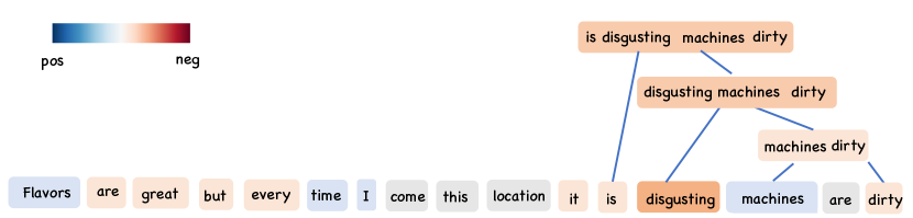
(b) A positive example “Flavors are great but every time I come this location it is disgusting machines are dirty.”

Figure 10: PE for BERT on two examples from Yelp dataset.

Appendix C Implementation Details

In this work, all language models are implemented by Transformers. All our experiments are performed on one A800. The results are reported with 5 random seeds.

For fine tuning the projection matrix $\boldsymbol{P}_{c}$, we iterate 5 epochs using RiemanianAdam optimizer and learning rate is initialized as 1e-3, the batch size is 32. For fine tuning the projection matrix $\boldsymbol{P}_{s}$, we use the Penn Treebank dataset we iterate 40 epochs using Adam optimizer and learning rate is initialized as 1e-3. We set $d_{out}$ as 64. We use grid search to search $\alpha_{1},\alpha_{2},\beta_{1},\beta_{2}\in\{0,0.1,0.2,0.3,0.4,0.5\}$.

References

- Abnar and Zuidema (2020) Samira Abnar and Willem Zuidema. 2020. Quantifying attention flow in transformers. In Proceedings of the 58th Annual Meeting of the Association for Computational Linguistics.
- Chen et al. (2020) Hanjie Chen, Guangtao Zheng, and Yangfeng Ji. 2020. Generating hierarchical explanations on text classification via feature interaction detection. In Proceedings of the 58th Annual Meeting of the Association for Computational Linguistics.
- Chen et al. (2023) Qian Chen, Taolin Zhang, Dongyang Li, and Xiaofeng He. 2023. Cidr: A cooperative integrated dynamic refining method for minimal feature removal problem.
- Dasgupta (2016) Sanjoy Dasgupta. 2016. A cost function for similarity-based hierarchical clustering. In Proceedings of the Forty-Eighth Annual ACM Symposium on Theory of Computing.
- Devlin et al. (2019) Jacob Devlin, Ming-Wei Chang, Kenton Lee, and Kristina Toutanova. 2019. BERT: Pre-training of deep bidirectional transformers for language understanding. In NAACL2018.
- DeYoung et al. (2020) Jay DeYoung, Sarthak Jain, Nazneen Fatema Rajani, Eric Lehman, Caiming Xiong, Richard Socher, and Byron C. Wallace. 2020. ERASER: A benchmark to evaluate rationalized NLP models. In Proceedings of the 58th Annual Meeting of the Association for Computational Linguistics.
- Dhamdhere et al. (2020) Kedar Dhamdhere, Ashish Agarwal, and Mukund Sundararajan. 2020. The shapley taylor interaction index. In Proceedings of the 37th International Conference on Machine Learning.
- Enguehard (2023) Joseph Enguehard. 2023. Sequential integrated gradients: a simple but effective method for explaining language models. In Findings of the Association for Computational Linguistics: ACL 2023.
- Enouen and Liu (2022) James Enouen and Yan Liu. 2022. Sparse interaction additive networks via feature interaction detection and sparse selection. In Advances in Neural Information Processing Systems.
- Ferrando et al. (2022) Javier Ferrando, Gerard I. Gállego, and Marta R. Costa-jussà. 2022. Measuring the mixing of contextual information in the transformer. In Proceedings of the 2022 Conference on Empirical Methods in Natural Language Processing.
- Ganea et al. (2018) Octavian Ganea, Gary Becigneul, and Thomas Hofmann. 2018. Hyperbolic neural networks. In Advances in Neural Information Processing Systems.
- Geva et al. (2021) Mor Geva, Roei Schuster, Jonathan Berant, and Omer Levy. 2021. Transformer feed-forward layers are key-value memories. In Proceedings of the 2021 Conference on Empirical Methods in Natural Language Processing.
- Graham and Hell (1985) Ronald L Graham and Pavol Hell. 1985. On the history of the minimum spanning tree problem. Annals of the History of Computing.
- Guidotti et al. (2018) Riccardo Guidotti, Anna Monreale, Salvatore Ruggieri, Franco Turini, Fosca Giannotti, and Dino Pedreschi. 2018. A survey of methods for explaining black box models.
- He et al. (2022) Junxian He, Chunting Zhou, Xuezhe Ma, Taylor Berg-Kirkpatrick, and Graham Neubig. 2022. Towards a unified view of parameter-efficient transfer learning. In International Conference on Learning Representations.
- Hewitt and Manning (2019) John Hewitt and Christopher D. Manning. 2019. A structural probe for finding syntax in word representations. In Proceedings of the 2019 Conference of the North American Chapter of the Association for Computational Linguistics: Human Language Technologies, Volume 1 (Long and Short Papers).
- Honnibal and Montani (2017) Matthew Honnibal and Ines Montani. 2017. spaCy 2: Natural language understanding with Bloom embeddings, convolutional neural networks and incremental parsing. To appear.
- Jin et al. (2020) Xisen Jin, Zhongyu Wei, Junyi Du, Xiangyang Xue, and Xiang Ren. 2020. Towards hierarchical importance attribution: Explaining compositional semantics for neural sequence models. In International Conference on Learning Representations.
- Ju et al. (2023) Yiming Ju, Yuanzhe Zhang, Kang Liu, and Jun Zhao. 2023. A hierarchical explanation generation method based on feature interaction detection. In Findings of the Association for Computational Linguistics: ACL 2023.
- Kochurov et al. (2017) Max Kochurov, Rasul Karimov, and Serge Kozlukov. 2017. Geoopt: Riemannian optimization in pytorch. In International Conference on Machine Learning, GRLB Workshop.
- Kokalj et al. (2021) Enja Kokalj, Blaž Škrlj, Nada Lavrač, Senja Pollak, and Marko Robnik-Šikonja. 2021. BERT meets shapley: Extending SHAP explanations to transformer-based classifiers. In Proceedings of the EACL Hackashop on News Media Content Analysis and Automated Report Generation.
- Li and Roth (2002) Xin Li and Dan Roth. 2002. Learning question classifiers. In COLING 2002: The 19th International Conference on Computational Linguistics.
- Lipton (2018) Zachary C. Lipton. 2018. The mythos of model interpretability: In machine learning, the concept of interpretability is both important and slippery. Queue.
- Lu et al. (2023) Xiaolei Lu, Jianghong Ma, and Haode Zhang. 2023. Asymmetric feature interaction for interpreting model predictions. In Findings of the Association for Computational Linguistics: ACL 2023.
- Mardaoui and Garreau (2021) Dina Mardaoui and Damien Garreau. 2021. An analysis of lime for text data. In Proceedings of The 24th International Conference on Artificial Intelligence and Statistics.
- Masoomi et al. (2022) Aria Masoomi, Davin Hill, Zhonghui Xu, Craig P Hersh, Edwin K. Silverman, Peter J. Castaldi, Stratis Ioannidis, and Jennifer Dy. 2022. Explanations of black-box models based on directional feature interactions. In International Conference on Learning Representations.
- Mitchell et al. (2022) Rory Mitchell, Joshua Cooper, Eibe Frank, and Geoffrey Holmes. 2022. Sampling permutations for shapley value estimation. J. Mach. Learn. Res.
- Modarressi et al. (2023) Ali Modarressi, Mohsen Fayyaz, Ehsan Aghazadeh, Yadollah Yaghoobzadeh, and Mohammad Taher Pilehvar. 2023. DecompX: Explaining transformers decisions by propagating token decomposition. In Proceedings of the 61st Annual Meeting of the Association for Computational Linguistics (Volume 1: Long Papers).
- Owen (2013) Guillermo Owen. 2013. Game theory. Emerald Group Publishing.
- Pang and Lee (2005) Bo Pang and Lillian Lee. 2005. Seeing stars: Exploiting class relationships for sentiment categorization with respect to rating scales. In Proceedings of the 43rd Annual Meeting of the Association for Computational Linguistics (ACL’05).
- Qiang et al. (2022) Yao Qiang, Deng Pan, Chengyin Li, Xin Li, Rhongho Jang, and Dongxiao Zhu. 2022. Attcat: Explaining transformers via attentive class activation tokens. In Advances in Neural Information Processing Systems.
- Ribeiro et al. (2016) Marco Tulio Ribeiro, Sameer Singh, and Carlos Guestrin. 2016. "why should i trust you?": Explaining the predictions of any classifier. In Proceedings of the 22nd ACM SIGKDD International Conference on Knowledge Discovery and Data Mining.
- Sanyal and Ren (2021) Soumya Sanyal and Xiang Ren. 2021. Discretized integrated gradients for explaining language models. In Proceedings of the 2021 Conference on Empirical Methods in Natural Language Processing.
- Shapley et al. (1953) Lloyd S Shapley et al. 1953. A value for n-person games.
- Shrikumar et al. (2017a) Avanti Shrikumar, Peyton Greenside, and Anshul Kundaje. 2017a. Learning important features through propagating activation differences. In Proceedings of the 34th International Conference on Machine Learning - Volume 70.
- Shrikumar et al. (2017b) Avanti Shrikumar, Peyton Greenside, Anna Shcherbina, and Anshul Kundaje. 2017b. Not just a black box: Learning important features through propagating activation differences.
- Singh et al. (2019) Chandan Singh, W. James Murdoch, and Bin Yu. 2019. Hierarchical interpretations for neural network predictions. In International Conference on Learning Representations.
- Snell et al. (2017) Jake Snell, Kevin Swersky, and RichardS. Zemel. 2017. Prototypical networks for few-shot learning. In Neural Information Processing Systems,Neural Information Processing Systems.
- Sundararajan et al. (2017) Mukund Sundararajan, Ankur Taly, and Qiqi Yan. 2017. Axiomatic attribution for deep networks. In International conference on machine learning.
- Tsang et al. (2020) Michael Tsang, Sirisha Rambhatla, and Yan Liu. 2020. How does this interaction affect me? interpretable attribution for feature interactions. In Advances in Neural Information Processing Systems.
- Vaswani et al. (2017) Ashish Vaswani, Noam Shazeer, Niki Parmar, Jakob Uszkoreit, Llion Jones, Aidan N. Gomez, Łukasz Kaiser, and Illia Polosukhin. 2017. Attention is all you need. In NIPS2017.
- Wang and Wang (2018) Dingkang Wang and Yusu Wang. 2018. An improved cost function for hierarchical cluster trees.
- Xilong et al. (2023) Zhang Xilong, Liu Ruochen, Liu Jin, and Liang Xuefeng. 2023. Interpreting positional information in perspective of word order. In Proceedings of the 61st Annual Meeting of the Association for Computational Linguistics (Volume 1: Long Papers).
- Zhang et al. (2021a) Die Zhang, Hao Zhang, Huilin Zhou, Xiaoyi Bao, Da Huo, Ruizhao Chen, Xu Cheng, Mengyue Wu, and Quanshi Zhang. 2021a. Building interpretable interaction trees for deep nlp models.
- Zhang et al. (2021b) Die Zhang, Hao Zhang, Huilin Zhou, Xiaoyi Bao, Da Huo, Ruizhao Chen, Xu Cheng, Mengyue Wu, and Quanshi Zhang. 2021b. Building interpretable interaction trees for deep nlp models. Proceedings of the AAAI Conference on Artificial Intelligence.
- Zhang et al. (2015) Xiang Zhang, Junbo Zhao, and Yann LeCun. 2015. Character-level convolutional networks for text classification. In Advances in Neural Information Processing Systems.