Galactic dynamics in the presence of scalaron: A perspective from $\boldsymbol{f(R)}$ gravity

Abstract

We consider $f(R)$ modified gravity with the chameleon mechanism as an alternative approach to address the dark matter issue on the galactic scale. Metric formalism of $f(R)$ theory is considered in this study. A mathematical transformation tool called conformal transformation which transforms the action from Jordan to Einstein frame is employed to simplify the fourth-order modified field equation and to describe the extra degree of freedom $f_{R}$ by using a minimally coupled scalar field (scalaron) showing the chameleonic character. Then, we examine the viability of a newly introduced $f(R)$ gravity model on behalf of the chameleonic behavior of the scalaron. The model analyzes this behavior of the scalaron successfully with the singularity correction. Further, we consider a test particle (star) in a static, spherically symmetric spacetime to investigate the importance of the scalaron in galactic dynamics. In the non-relativistic limit, the rotational velocity equation for the particle with scalaron contribution is derived. This contribution is found to be model dependent. We generate the rotation curves using the velocity equation and fit the predicted curves to observational data of a set of thirty seven sample galaxies of different categories. The curves are fitted based on two fitting parameters $M_{0}$ and $r_{c}$. The fitting shows good agreement of the prediction with the observed data.

I Introduction

The captivating enigma of dark matter (DM) and the accelerated expansion of the Universe are two formidable challenges of modern astrophysics and cosmology. Behaviors of observed galactic rotation curves 1970_Rubin ; 1978_Rubin ; 1983_Rubin and gravitational lensing 2011_Gar ; 2010_Massey in galaxies and their clusters manifest the mass discrepancy in them and suggest the need for DM as a major matter component in the Universe. However, there is currently no experimental evidence supporting the existence of this elusive missing matter and the interpretation of late time acceleration of the Universe as well. These two so-called greatest puzzles of modern times have stimulated the scientific community to think about the modifications of Einstein’s theory of General relativity (GR) and upshot the modified theories of gravity (MTGs) 2022_Shankar ; 1983_Milikan ; 2008_capoz ; 2010_harko ; 2011_harko ; 2011_Capoz ; 2021_Atayde . These theories are the consequences of the modification of gravity part of Einstein-Hilbert (EH) action and can be treated as an alternative approach for explaining the issues of DM 2006_Sobouti ; 2008_Harko ; 2010_Harko ; 2011_Gegurgel ; 2016_Zaregonbadi ; 2021_Nashiba ; 2023_Nashiba ; 2018_Finch ; 2023_Shabani as well as dark energy (DE), the dominant unknown component of mass-energy that is supposed to be responsible for the present accelerated expansion of the Universe 2013_Chakraborti ; 2008_capozz ; 2016_Joyce ; 2002_Peebles . $f(R)$ gravity 1970_Buchd ; 1980_starobinsky ; 2020_dhruba ; 2007_sawiki , $f(R,T)$ gravity 2011_harko ; 2013_alva , Gauss-Bonnet gravity 1971_David ; 2005_nojiri , Scalar-tensor theories 2003_chiba ; 2007_martin , Braneworld models 2011_sahidi etc. are some widely studied gravity theories as alternatives to GR. Among different MTGs, the simplest modification of GR is the $f(R)$ theory of gravity, proposed by H. A. Buchdahl in $1970$ through the replacement of the Ricci scalar $R$ in the EH action with an arbitrary function $f(R)$ of it 1970_Buchd . In this theory, field equations can be derived from the action using mainly two approaches: one is the metric formalism in which the affine connection $\Gamma^{\rho}_{\alpha\beta}$ depends on the metric $g_{\mu\nu}$ and the field equations are obtained by varying the action with respect to the metric only. Another is the Palatini formalism in which the field equations are derived from the variation of the action treating affine connection and the metric as independent variables 2010_felice . Such covariant modifications of GR always introduce an extra degree of freedom besides the tensor degree of freedom. We restrict ourselves to metric $f(R)$ theory in this work. This theory can be reformulated as a scalar-tensor theory by describing this additional degree of freedom as a scalar field called scalaron 2006_Faulkner . Indeed, it is equivalent to a scalar-tensor theory if it is transformed to the Einstein frame via conformal transformation 2008_tamaki ; 2012_cliftone ; 2015_joyce ; 2014_terukina ; 2016_koyama ; 2018_burrage ; 2007_Chiba . Under this transformation the scalaron field couples with matter minimally and acquires effective mass that depends sensitively on the density of the environment. The scalaron field exhibiting such a local matter density dependent physical property is referred to as a chameleon field and the mechanism involved is called the chameleon mechanism 2004_Khoury ; 2004_Khoury2 . It is a screening mechanism in which the scalaron changes its properties to fit the surroundings where the field is allowed to exhibit significant mass in dense environments, such as within the solar system, and less mass in low density regions, such as on cosmological scales. In high density surroundings, the force induced by the scalaron field is suppressed while in low density localities it mediates a force of gravitational strength extending its impacts over a long range 2013_Khoury ; 2010_Hinter . Such a low-mass scalar field may be a genuine substitute for DM.

A range of studies have been undertaken to investigate the scalaron as an alternative to DM and DE in MTGs. Especially, the effectiveness of chameleonically viable $f(R)$ models in mimicking the DM component of the Universe was explored at different scales. Ref. 2018_verma has explained the DM problem in chameleon $f(R)$ gravity by considering a model of the from $f(R)=R^{(1+\delta)}/R^{\delta}_{c}$ and suggested that behaviour of the scalaron derived from this model makes it suitable to mimic as DM. The study of DM taking into account the screening mechanism in the Starobinsky model is addressed in Ref. 2017_katsu . This study has analysed three different possible ways for revealing light scalaron to be a DM candidate and also estimated its lifetime by investigating the coupling between the scalaron and standard model particles. Refs. 2018_kat ; 2021_Nashiba have illustrated DM based on chameleonic features of scalaon. It is suggested in Ref. 2021_Nashiba that the mass of the scalaron can be found to be close to the mass of ultralight axions, so it can be treated as a mimicking DM candidate. Refs. 2012_Burikham investigated the effects of a chameleon scalar field on rotation curves of certain late-type low surface brightness (LSB) galaxies and observed a cuspier rotation curve for each galaxy. Some other investigations 2012_mann ; 2021_Shtanov ; 2018_Naik ; 2020_Li ; 2006_brown have been conducted by analyzing the chameleon scalar field to address DM issues. These works have motivated us to consider a study for the explanation of this exotic matter component by exploring the chameleonic behaviour of a recently introduced $f(R)$ gravity model 2020_dhruba ; 2022_dhruba . Specifically, in this study, we intend to check the chameleonic viability of this model of $f(R)$ gravity by examining the characteristics of its scalar degree of freedom (scalaron). Our principal focus of this study is to investigate the impact of scalaron on galactic dynamics taking into consideration of chameleon mechanism via conformal transformation in metric $f(R)$ gravity theory. With this objective, we first derive field equations of metric $f(R)$ gravity. Then by conformal transformation, the fourth-order equations generated by the theory are simplified to second-order equations through the introduction of a scalar field that shows chameleonic features. We study this feature of the field shown by the model with a correction of the singularity problem usually suffered by $f(R)$ gravity models 2021_Nashiba . The singularity correction makes scalaron reasonably light in denser regions, such as in the galactic center, which may mitigate the suppression of the field due to its induced force. Using the singularity corrected model, we obtain rotational velocity with scalaron contribution term for test particles moving around galaxies in stable circular orbits. The rotation curves thus predicted by the theory are then fitted with observations of some samples of high surface brightness (HSB), LSB and dwarf galaxies, and achieve well-fitted rotation curves almost for all sample galaxies.

The work is organized as follows. In Section II, we derive the field equations of the $f(R)$ gravity and then via conformal transformation the minimal coupling of a scalar field (scalaron) to non-relativistic matter is presented. Also, the equation of motion of the scalaron, its effective potential and expression for mass are derived. In Section III, by considering a new f($R$) gravity model 2020_dhruba ; 2022_dhruba as mentioned above, the chameleonic behavior of the scalaron is outlined. The singularity problem suffered by the model is also discussed in this section. In Section IV, assuming a static, spherically symmetric spacetime the orbital motion of a test particle in the presence of the scalaron is presented. Finally, we conclude our work in Section V with some future prospects. In this work, we set $c=\hbar=1$ and adopt the metric signature as $(-,+,+,+)$.

II $\boldsymbol{f(R)}$ Gravity Field Equations and Conformal Transformation

II.1 Field equations in metric formalism

To derive field equations in metric formalism, we proceed from the action of $f(R)$ gravity, which is given as  2010_felice ; 2010_sotiriou

$$S=\frac{1}{2\kappa^{2}}\int\!d^{4}x\,\sqrt{-\,g}\,{f(R)}+S_{m}\left(g_{\mu\nu},\psi\right),$$ (1)

where $g$ is the determinant of the metric $g_{\mu\nu}$, $\kappa^{2}=8\pi G=M_{pl}^{-2}$, $M_{pl}$ is the reduced Plank mass $\approx 2.4\times 10^{18}$ GeV, and $S_{m}(g_{\mu\nu},\psi)=\int\!d^{4}x\,\sqrt{-\,g}\,\mathcal{L}_{m}(g_{\mu\nu},\psi)$ is the matter action with the non-relativistic matter field $\psi$. The Ricci scalar $R$ is defined as $R=g^{\mu\nu}R_{\mu\nu}$, where the Ricci tensor $R_{\mu\nu}$ is expressed in the from:

$$R_{\mu\nu}=R^{\sigma}_{\mu\sigma\nu}=\partial_{\sigma}\Gamma^{\sigma}_{\mu\nu}-\partial_{\nu}\Gamma^{\sigma}_{\mu\sigma}+\Gamma^{\lambda}_{\mu\nu}\Gamma^{\sigma}_{\lambda\sigma}-\Gamma^{\lambda}_{\mu\sigma}\Gamma^{\sigma}_{\lambda\nu}.$$ (2)

The variation of action (1) with respect to metric $g_{\mu\nu}$ results in the field equations of the metric formalism of $f(R)$ gravity as given by

$$f_{R}R_{\mu\nu}-\frac{1}{2}\,g_{\mu\nu}f(R)-\big{[}\nabla_{\mu}\nabla_{\nu}-g_{\mu\nu}\,\square\big{]}\,f_{R}=\kappa^{2}\,T_{\mu\nu}.$$ (3)

Here, $f_{R}=df/dR$, $\nabla_{\mu}$ is the covariant derivative connected with the Levi-Civita connection of metric $g_{\mu\nu}$, $\square=\nabla^{\mu}\nabla_{\mu}$ is the Laplace operator in four dimensions and $T_{\mu\nu}$ is the energy-momentum tensor which satisfies the condition: $\nabla^{\mu}T_{\mu\nu}=0$, and usually it is given by

$$T_{\mu\nu}=-\,\frac{2}{\sqrt{-g}}\,\frac{\delta S_{m}}{\delta g^{\mu\nu}}\equiv-\,\frac{2}{\sqrt{-g}}\,\frac{\delta(\sqrt{-g}\,\mathcal{L}_{m})}{\delta g^{\mu\nu}}.$$ (4)

The field equations (3) in the form of Einstein field equations can be written as

$$G_{\mu\nu}=\frac{\kappa^{2}\,T_{\mu\nu}}{f_{R}}+g_{\mu\nu}\frac{f(R)-Rf_{R}}{2f_{R}}+\frac{\nabla_{\mu}\nabla_{\nu}f_{R}-g_{\mu\nu}\,\square f_{R}}{f_{R}}=\frac{\kappa^{2}}{f_{R}}\left(T_{\mu\nu}+T_{\mu\nu}^{eff}\right),$$ (5)

where $T_{\mu\nu}^{eff}$ is the effective energy-momentum tensor of the following form:

$$T_{\mu\nu}^{eff}=\frac{1}{\kappa^{2}}\left[g_{\mu\nu}\frac{f(R)-Rf_{R}}{2}+\big{(}\nabla_{\mu}\nabla_{\nu}-g_{\mu\nu}\,\square\big{)}f_{R}\right].$$ (6)

Further, the modified field equations (5) may also take the form:

$$f_{R}\left[G_{\mu\nu}+G_{\mu\nu}^{d}\right]=\kappa^{2}\,T_{\mu\nu},$$ (7)

where

$$G_{\mu\nu}^{d}=\frac{1}{f_{R}}\left[g_{\mu\nu}\frac{Rf_{R}-f(R)}{2}-\big{(}\nabla_{\mu}\nabla_{\nu}-g_{\mu\nu}\square\big{)}f_{R}\right].$$

is the deviated part of the Einstein tensor that appears due to the change in the curvature introduced by the $f(R)$ gravity. The effective energy-momentum tensor is also emerged due to the same reason, i.e. the change of the behaviour of curvature in $f(R)$ gravity.

The existence of the last two terms on the left hand side of equations (3) expresses them as fourth-order partial differential equations. The trace of equations (3) is obtained as

$$3\,\square f_{R}+f_{R}\,R-2\,f(R)=\kappa^{2}T,$$ (8)

where $T=T_{\mu}^{\mu}$ is the trace of the energy-momentum tensor and $\square f_{R}=\partial_{\mu}(\sqrt{-g}\,g^{\mu\nu}\partial_{\nu}f_{R})/\sqrt{-g}$. Equation (8) is the equation of motion for $f_{R}$ that determines the dynamics of $f_{R}$. It shows that the Ricci scalar $R$ is dynamic. With $f(R)$ as a linear function of $R$, $f_{R}$ is constant and hence $\square f_{R}=0$. In this case, the theory reduces to GR leading the equation (8) as $R=-\,\kappa^{2}T$, implying the direct dependence of Ricci scalar on matter. Instead, in $f(R)$ theory $\square f_{R}$ does not vanish. It signifies that the theory includes an extra propagating degree of freedom $f_{R}$, called the scalar degree of freedom that characterizes the modification of gravity and plays a central role in explaining the galactic dynamics without dark matter 2017_katsu ; 2018_verma ; 2012_li . With this conformity, we consider a transformation of the metric from the Jordan frame to the Einstein frame through the conformal transformation in the following subsection to identify the additional degree of freedom of $f(R)$ theory conveniently in an explicit form.

II.2 Conformal transformation

Conformal transformation is a mathematical technique used expediently to simplify the equations of motion in the Jordan frame into an amenable form 1984_whitt . In fact, it is a tool that physicists generally use for a better understanding of the implications of MTGs and their connection to the standard framework of GR. Through a conformal transformation, the higher-order and non-minimally coupled terms can always be shown as the sum of the Einstein gravity and one or more minimally coupled scalar field(s) 2011_Capoz . In the case of the fourth-order gravity when undergoing this transformation, gives one scalar field with the Einstein gravity. Before performing such a transformation we recast the action (1) in the following form 2010_felice :

$$S=\int\!d^{4}x\,\sqrt{-\,g}\,\left[\frac{Rf_{R}}{2\kappa^{2}}-X(R)\right]+\int\!d^{4}x\,\sqrt{-\,g}\,\mathcal{L}_{m}\left(g_{\mu\nu},\psi\right),$$ (9)

where

$$X(R)=\frac{1}{2\kappa^{2}}\big{[}Rf_{R}-f(R)\big{]}.$$ (10)

Equation (10) can be treated as the potential of an auxiliary scalar field defined in the Jordan frame 2021_Nashiba ; 2010_sotiriou ; 2020_vel . This potential is non-zero only when $f_{R}\neq 1$. When $f_{R}=1$, it becomes zero and hence the theory reduces to GR. We consider now the following conformal transformation that reduces the fourth-order non-minimally coupled field equations (3) into a minimally coupled tractable form through the transition of the Jordan frame metric $g_{\mu\nu}$ to the Einstein frame metric $\tilde{g}_{\mu\nu}$ as 2010_felice ; 2007_Faraoni ; 2014_spo ; 2009_dab ; 1999_far

$$g_{\mu\nu}\rightarrow\tilde{g}_{\mu\nu}=\Omega^{2}g_{\mu\nu},$$ (11)

where $\Omega^{2}$ is a non-vanishing regular function called the conformal factor. Under transformation rule (11) the Ricci scalars $R$ and $\tilde{R}$ in these two respective frames are related by

$$R=\Omega^{2}\left[\tilde{R}+6\,\square\,(\ln\Omega)-6\,\tilde{g}^{\mu\nu}\nabla_{\mu}\,(\ln\Omega)\,\nabla_{\nu}\,(\ln\Omega)\right].$$ (12)

Also, the determinants of the metric tensors in the two frames hold the following relation:

$$\sqrt{-g}=\Omega^{-4}\sqrt{-\tilde{g}}\,.$$ (13)

Using equations (9), (12) and (13), and also Gauss’s theorem the action in Einstein’s frame is derived as given below:

$$S_{E}=\int\!d^{4}x\,\sqrt{-\tilde{g}}\,\Big{[}\frac{1}{2\kappa^{2}}f_{R}\,\Omega^{-2}\big{\{}\tilde{R} -6\,\tilde{g}^{\mu\nu}\nabla_{\mu}(\ln\Omega)\nabla_{\nu}(\ln\Omega)\big{\}}-\frac{X(f_{R})}{\Omega^{4}}\Big{]}$$

$$+\int\!d^{4}x\;\Omega^{-4}\sqrt{-\tilde{g}}\,\mathcal{L}_{m}\left(\Omega^{-2}\,\tilde{g}_{\mu\nu},\psi\right).$$ (14)

At this stage, we are in a position to introduce a new scalar field called scalaron $\phi$ defined by 2013_kob

$$\phi=\frac{1}{\kappa}\,\sqrt{\frac{3}{2}}\ln f_{R}.$$ (15)

This field corresponds to an extra scalar degree of freedom $f_{R}$ in $f(R)$ theory as

$$f_{R}=e^{\sqrt{\frac{2}{3}}k\phi}.$$ (16)

Using the scalar field defined in equation (15) and choosing the conformal factor $\Omega^{2}=f_{R}$, the action (14) in Einstein’s frame can be written in the form:

$$S_{E}=\frac{1}{2\kappa^{2}}\!\int\!d^{4}x\,\sqrt{-\tilde{g}}\,\tilde{R} +\int\!d^{4}x\,\sqrt{-\tilde{g}}\,\left[-\frac{1}{2}\,\tilde{g}^{\mu\nu}\partial_{\mu}\phi\,\partial_{\nu}\phi-V(\phi)\right]$$

$$+\int\!d^{4}x\;\frac{\sqrt{-\tilde{g}}}{f_{R}^{\,2}}\,\mathcal{L}_{m}\left(f_{R}(\phi)^{-1}\,\tilde{g}_{\mu\nu},\psi\right).$$ (17)

Here, we may write $f_{R}(\phi)^{-1}=e^{2\beta\kappa\phi}$ which gives constant coupling factor $\beta=-1/\sqrt{6}$. It indicates that the scalar field is directly coupled to matter field $\psi$ with a constant coupling $\beta$ in the Einstein frame. Further, $V(\phi)$ represents the potential of the scalaron field defined by

$$V(\phi)=\frac{X}{f_{R}^{\,2}}=\frac{1}{2\kappa^{2}}\left[\frac{Rf_{R}-f(R)}{f_{R}^{\,2}}\right].$$ (18)

Equation (17) shows that $f(R)$ gravity can be expressed by means of GR along with the additional scalar field, the scalaron, that holds noteworthy significance in the theory.

II.3 Equation of motion of scalaron and its mass

Variation of action (17) with respect to $\phi$ gives the following equation:

$$\tilde{\square}\,\phi-\dfrac{dV(\phi)}{d\phi}+\frac{1}{\sqrt{-\tilde{g}}}\frac{\partial(\sqrt{-g}\,\mathcal{L}_{m})}{\partial\phi}=0,$$ (19)

where

$$\tilde{\square}=\frac{1}{\sqrt{-\tilde{g}}}\,\partial_{\mu}(\sqrt{-\tilde{g}}\,\tilde{g}^{\mu\nu}\partial_{\nu}).$$

Again, the derivative factor of the last term on the left-hand side of equation (19) can be expressed as

$$\frac{\partial(\sqrt{-g}\,\mathcal{L}_{m})}{\partial\phi}=-\,\frac{\sqrt{-g}}{2}\left(-\,\frac{2}{\sqrt{-g}}\,\frac{\delta(\sqrt{-g}\,\mathcal{L}_{m})}{\delta g^{\mu\nu}}\right)\frac{\partial g^{\mu\nu}}{\partial\phi}=-\,\frac{\sqrt{-g}}{2}\,T_{\mu\nu}\,\frac{\partial g^{\mu\nu}}{\partial\phi}.$$ (20)

Also we have,

$$\tilde{T}_{\mu\nu}=-\,\frac{2}{\sqrt{-\tilde{g}}}\,\frac{\delta(\sqrt{-g}\,\mathcal{L}_{m})}{\delta\tilde{g}^{\mu\nu}}=\frac{T_{\mu\nu}}{f_{R}}.$$ (21)

Use of equations (11) in contravariant form, and equations (13) and (21) in equation (20) yields

$$\frac{\partial(\sqrt{-g}\,\mathcal{L}_{m})}{\partial\phi}=-\,\frac{\sqrt{-\tilde{g}}}{2f_{R}}\,\frac{df_{R}}{d\phi}\,\tilde{T}_{\mu}^{\mu}.$$ (22)

From $\tilde{T}_{\mu}^{\mu}=T_{\mu}^{\mu}/f_{R}^{\,2}$, the relation between the trace of the energy-momentum tensors in two frames and equation (22) together with relation (16) we can rewrite scalaron’s equation of motion (19) as

$$\tilde{\square}\,\phi-\frac{dV_{eff}}{d\phi}=0,$$ (23)

where

$$\dfrac{dV_{eff}(\phi)}{d\phi} =\dfrac{dV(\phi)}{d\phi}+\frac{\kappa}{\sqrt{6}}\,\tilde{T}_{\mu}^{\mu}$$

$$=\dfrac{dV(\phi)}{d\phi}+\frac{\kappa}{\sqrt{6}}\,e^{-2\sqrt{\frac{2}{3}}\kappa\phi}\,T_{\mu}^{\mu}.$$ (24)

$V_{eff}(\phi)$ refers the effective potential of the scalaron field. Equation (23) shows in conjunction with equation (24) that scalaron couples to the matter field in the Einstein frame with a constant coupling strength $1/\sqrt{6}$ as mentioned earlier. In the Jordan frame, this coupling strength decreases exponentially with the increasing scalaron field value. Also it should be noted that as matter moves on geodesic of Jordan frame metric, the Einstein frame energy-momentum tensor $\tilde{T}_{\mu\nu}$ is not covariantly conserved, i.e. $\tilde{\nabla}_{\mu}\tilde{T}_{\mu\nu}\neq 0$ 2018_burrage . Assuming the energy-momentum tensor for an ideal non-relativistic matter we obtain $T_{\mu}^{\mu}=-\rho$, the local non-relativistic matter density, which results in $V_{eff}$ as

$$V_{eff}=V(\phi)+\frac{1}{4}\,\rho\,e^{-2\sqrt{\frac{2}{3}}\kappa\phi}.$$ (25)

The presence of the second term in equation (25) indicates that the dynamics of the scalaron described by the equation (23) is influenced by the matter density of the environment. In high-density environments propagation of the scalaron is ceased and it is regarded to be short-ranged while in low-density regions smaller mass makes the field long-ranged 2016_koyama . Consequently, the effective potential results in environment-density dependent scalaron mass $m_{\phi}$ as the square of $m_{\phi}$ corresponds to the second order derivative of effective potential at the minimum of the field value $\phi_{0}$. So, we obtain the mass of the scalaron by differentiating equation (24) with respect to $\phi$ at $\phi=\phi_{0}$ as

$$m_{\phi}^{2}=\dfrac{d^{2}V_{eff}(\phi)}{d\phi^{2}}=\dfrac{d^{2}V(\phi_{0})}{d\phi^{2}}+\frac{2\kappa^{2}\rho}{3}e^{-2\sqrt{\frac{2}{3}}\kappa\phi_{0}}.$$ (26)

From equation (26) it is found that the potential $V(\phi)$ is not only the determining factor of the scalaron mass, it is strongly affected by the matter density $\rho$ of surroundings as mentioned above. The scalaron becomes heavier in high-density regions and lighter where density is low. The development of such a dependency of scalaron mass on local matter density is a feature of the chameleon mechanism which characterizes the scalaron as a chameleon field. To explicitly express the factor contributed by the potential $V(\phi)$ to the scalaron mass and also to express the scalaron mass in a suitable form we proceed as follows. From equations (15) and (18) we may write,

$$\dfrac{dV(\phi)}{dR} =\frac{1}{2\kappa^{2}}\,\frac{2f(R)f_{RR}-Rf_{R}f_{RR}}{f_{R}^{\,3}}.$$ (27)

$$\dfrac{d\phi}{dR} =\frac{1}{\kappa}\,\sqrt{\frac{3}{2}}\frac{f_{RR}}{f_{R}}.$$ (28)

These two equations provide us the derivatives of $V(\phi)$ with respect to $\phi$ as

$$\dfrac{dV(\phi)}{d\phi}=\frac{1}{\sqrt{6}\,\kappa}\,\frac{2f(R)-Rf_{R}}{f_{R}^{\,2}}.$$ (29)

From this equation, we may obtain,

$$\dfrac{d^{2}V(\phi)}{d\phi^{2}}=\frac{1}{3f_{RR}}\left[1+\frac{Rf_{RR}}{f_{R}}-\frac{4f(R)f_{RR}}{f_{R}^{\,2}}\right].$$ (30)

It should be mentioned that at the minimum of the scalaron field value i.e., at $\phi=\phi_{0}$, the effective potential satisfies the condition $dV_{eff}(\phi_{0})/d\phi=0$, which turns the left-hand side of equation (24) to zero. Thus, inserting equations (15) and (29) into (24), the stationary condition satisfied by the minimum of potential is obtained as

$$2f(R_{0})-R_{0}\,f_{R}(R_{0})=\rho\kappa^{2},$$ (31)

where $R_{0}$ is the Ricci scalar corresponding to the minimum of the scalaron $\phi_{0}$. Using equations (30) and (31) we can write a general expression from equation (26) for $m_{\phi}^{2}$ at minimum field value in the form given below:

$$m_{\phi}^{2}=\frac{1}{3f_{RR}(R_{0})}\left[1-\frac{R_{0}f_{RR}(R_{0})}{f_{R}(R_{0})}\right].$$ (32)

This equation is useful to study scalaron mass for a specific $f(R)$ gravity model.

III Chameleon Mechanism in a New $\boldsymbol{f(R)}$ Gravity Model

In this section, we study the scalaron mass and its chameleonic behavior in a model specific case considering a recently proposed $f(R)$ gravity model 2020_dhruba ; 2022_dhruba . Also, we discuss in this section the associated singularity problem in $f(R)$ gravity theory and its correction for this particular model.

III.1 Chameleonic behavior of scalaron mass

The $f(R)$ gravity model we consider here, as mentioned above, is given by 2020_dhruba ; 2022_dhruba

$$f(R)=R-\frac{\alpha}{\pi}\,R_{c}\,\cot^{-1}\!\left(\frac{R_{c}^{2}}{R^{2}}\right)-\beta R_{c}\left[1-e^{-\frac{R}{R_{c}}}\right],$$ (33)

where $\alpha$, $\beta$ are two dimensionless positive constants and $R_{c}$ is a characteristic curvature constant having the dimension same as the curvature scalar. For this model (33), $f_{R}$ can be obtained as

$$f_{R}(R)=1-\frac{2\,\alpha R_{c}^{3}}{\pi R^{3}\left(1+\frac{R_{c}^{4}}{R^{4}}\right)}-\beta e^{-\frac{R}{R_{c}}}.$$ (34)

The curvature $R$ should have the same order as that of the trace of energy-momentum tensor $T_{\mu}^{\mu}$. Hence in a high-density region, it attains a greater value for which we may assume it is larger than the characteristic curvature value $R_{c}$. Thus assuming $R$ in large curvature limit, i.e. $R\gg R_{c}$, we can approximate equation (33) in this limit as

$$f(R)=R-\frac{\alpha R_{c}}{2}-\beta R_{c}.$$ (35)

On the other hand, in the case of equation (34) the large curvature condition emanates two small-valued terms viz. $2\alpha\pi^{-1}(R_{c}/R)^{3}$ and $\beta\exp(-R/R_{c})$. When these terms are compared for particular values of model parameters irrespective of $\alpha\geq\beta$ or $\alpha<\beta$, it is found that the term $\beta\exp(-R/R_{c})$ is dominating over $2\alpha\pi^{-1}(R_{c}/R)^{3}$. Therefore, for simplicity we consider the less dominating term to obtain a comparatively greater $f_{R}$ value. Under this consideration equation (34) reduces to

$$f_{R}(R)=1-\frac{2\alpha}{\pi}\frac{R_{c}^{3}}{R^{3}}.$$ (36)

The derivative of it appears as

$$f_{RR}(R)=\frac{6\,\alpha}{\pi}\frac{R_{c}^{3}}{R^{4}}.$$ (37)

Thus equation (31) which is a consequence of minimum effective potential ensues a relation between matter density and curvature as

$$R_{0}=R_{c}\big{(}\rho\kappa^{2}+\alpha R_{c}+2\beta R_{c}-\frac{2\alpha}{\pi}\,\big{)}^{1/3}.$$ (38)

This relation when used in equation (32), along with equations (36) and (37) for the respective $f_{R}(R_{0})$ and $f_{RR}(R_{0})$ terms, we obtain a local matter density dependent mass of the scalaron for the chosen model as

$$m_{\phi}^{2}=\frac{\pi R_{c}}{18\alpha}\left(\rho\kappa^{2}+\alpha R_{c}+2\beta R_{c}-\frac{2\alpha}{\pi}\right)^{\!4/3}\!\left[1-\frac{6\alpha}{\pi\left(\rho\kappa^{2}+\alpha R_{c}+2\beta R_{c}-\frac{2\alpha}{\pi}\right)-2\alpha}\right].$$ (39)

It is clear from equation (39) that the scalaron mass depends on matter density $\rho$ of the surrounding environment and it increases as a certain power function of density $\rho$. This behaviour of the scalaron mass with increasing $\rho$ confirms the chameleonic nature of the scalaron in the model we have considered for our study. We depict this particular behavior of scalaron mass in Fig. 1 for different values of model parameters by setting the characteristic curvature $R_{c}=1$ 2020_dhruba . It is also clear from this figure that the scalaron mass decreases with the increasing values of the model parameters $\alpha$ and $\beta$.

     

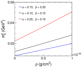
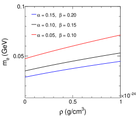
Figure 1: Relations between scalaron mass and matter density for three sets of model parameters $\alpha$ and $\beta$. The left plot is for the square of the scalaron mass and the right plot is for its linear form.

III.2 Singularity problem and its correction

It is seen from equations (18) and (33) that the scalaron potential is a function of curvature scalar $R$. By substituting equation (16) into equation (18), it can also be expressed as a function of the scalaron field $\phi$ where the relation between curvature scalar and scalaron field is given by

$$R=\left(\frac{2\alpha}{\pi}\right)^{1/3}\!\!\!\!R_{c}\left(1-e^{\sqrt{\frac{2}{3}}\kappa\phi}\right)^{-1/3}\!\!\!,$$ (40)

which is obtained from equations (16) and (36) in high curvature regime approximation consideration. Equation (40) hints to us about the curvature singulaity 2008_frolov . To understand this singularity problem in the specific new $f(R)$ gravity model chosen for our study, initially, we take the field-dependent scalaron potential without matter contribution which is attained in the form:

$$\frac{V(\phi)}{V_{0}}=\left[\frac{\alpha}{2}+\beta-\Big{(}\frac{2\alpha}{\pi}\Big{)}^{1/3}\Big{(}1-e^{\sqrt{\frac{2}{3}}\kappa\phi}\Big{)}^{2/3}\right]e^{-2\sqrt{\frac{2}{3}}\kappa\phi},$$ (41)

where $V_{0}=R_{c}/2\kappa^{2}$ is the normalization factor that normalizes the potential $V(\phi)$. The relation between $V(\phi)$ and $\phi$ given in equation (41) is shown in Fig. 2.

       

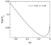
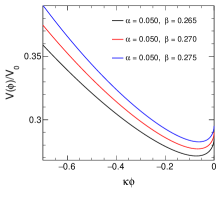
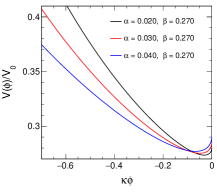
Figure 2: Variation of $V(\phi)$ with respect to $\kappa\phi$ for different values of model parameters $\alpha$ and $\beta$.

It is clear from the figure that the potential has no value for the positive $\kappa\phi$ value. In the left panel, we depict an explicit behavior of the potential as a function of the field and see that the potential decreases with increasing $\phi$. It reaches a minimum at $\phi\sim 0.1$ and then increases up to $\phi=0$. The other two panels illustrate that the minimum of the potential moves towards the higher field value for larger values of $\alpha$ and $\beta$. Also, the potential minimum uplifts noticeably for higher values of $\alpha$ and $\beta$.

Now, we consider the matter contribution to the potential as given by equation (25) and plot the behavior of the effective potential in Fig. 3 against the scalaron field for a positive matter density using the normalized equation as given below:

$$\frac{V_{eff}(\phi)}{V_{0}}=\left[\frac{\alpha}{2}+\beta-\Big{(}\frac{2\alpha}{\pi}\Big{)}^{1/3}\Big{(}1-e^{\sqrt{\frac{2}{3}}\kappa\phi}\Big{)}^{2/3}\!\!+\frac{1}{2R_{c}}\,\rho\kappa^{2}\right]e^{-2\sqrt{\frac{2}{3}}\kappa\phi}.$$ (42)

       

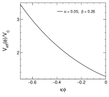
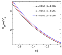
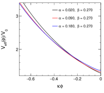
Figure 3: Variation of effective potential $V_{eff}(\phi)$ as a function of $\kappa\phi$ for different values of model parameters $\alpha$ and $\beta$ with the matter density $\rho=\rho_{c}$, where $\rho_{c}$ is the critical matter density of the Universe.

One can see from Fig. 3 that the presence of matter flattened the minimum of the potential and shifted it very close to $\phi=0$. In fact, the minimum can smoothly correspond to zero of the scalaron field. This $\phi\rightarrow 0$ correlates with the curvature singularity as hinted by equation (40) i.e., $R\rightarrow\infty$ when $\phi\rightarrow 0$, can be easily obtainable in the presence of matter. Ref. 2008_frolov suggested that the problem of curvature singularity is not unique to only a particular $f(R)$ gravity model, but it is endured by many infrared-modified $f(R)$ gravity models.

The above curvature singularity appeared in terms of the scalaron field potential in the high curvature regime can be removed by reforming the structure of the potential in this curvature regime 2018_kat ; 2009_kobay . This can be done by adding higher order correction term $\sigma R^{2}$ to the $f(R)$ model as follows:

$$f(R)=R-\frac{\alpha}{\pi}\,R_{c}\,\cot^{-1}\!\left(\frac{R_{c}^{2}}{R^{2}}\right)-\beta R_{c}\left[1-e^{-\frac{R}{R_{c}}}\right]+\sigma R^{2},$$ (43)

where $\sigma$ is a dimensionful constant. In the higher curvature regime equation (43) reduces to

$$f(R)=R-\frac{\alpha R_{c}}{2}-\beta R_{c}+\sigma R^{2}.$$ (44)

Also, after introducing the correction term we obtain $f_{R}$ and the relation between curvature $R$ and the scalaron field through conformal transformation respectively as follows:

$$f_{R}=1-\frac{2\alpha}{\pi}\frac{R_{c}^{3}}{R^{3}}+2\sigma R,$$ (45)

$$e^{\sqrt{\frac{2}{3}}\kappa\phi}=1-\frac{2\alpha}{\pi}\frac{R_{c}^{3}}{R^{3}}+2\sigma R.$$ (46)

The noteworthy feature of this equation is that contrary to the resolution provided by the equation (40), it results in $R\rightarrow\infty$ for $\phi\rightarrow\infty$. Equations (44), (45) and (46) configure the $R^{2}$ corrected normalized field potential as

$$\frac{V(\phi)}{V_{0}}=\left[\frac{\alpha}{2}+\beta-\frac{128\alpha}{\pi}R_{c}^{2}\sigma^{2}\big{(}e^{\sqrt{\frac{2}{3}}\kappa\phi}-1\big{)}^{-2}\!+\frac{1}{64\sigma R_{c}}\big{(}e^{\sqrt{\frac{2}{3}}\kappa\phi}-1\big{)}^{2}\right]e^{-2\sqrt{\frac{2}{3}}\kappa\phi}.$$ (47)

The potential given by this equation (47) is plotted as a function of $\kappa\phi$ with $\sigma=10^{-6}R_{c}^{-1}$ GeV^-2 and for different values of the parameters of the new $f(R)$ gravity model in the left panel of Fig. 4. The figure shows that the curvature modification dictates the potential to have its values mostly for the positive $\phi$. At $\phi=0$, $R$ takes a small value $\approx\left({{\alpha R_{c}^{3}}/{\pi\sigma}}\right)^{1/4}$ instead of infinity as expected.

         

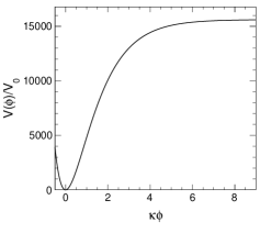
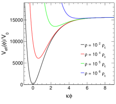
Figure 4: Variation of $R^{2}$ corrected potential $V(\phi)$ as a function of $\kappa\phi$ for the model parameters $\alpha=0.15$ and $\beta=0.05$ (left). Variation of $R^{2}$ corrected effective potential $V_{eff}(\phi)$ as a function of $\kappa\phi$ for $\alpha=0.05$, $\beta=0.25$ and four positive values of matter densities (right).

Then, by considering the matter contribution, the equation for the $R^{2}$ corrected effective potential is derived and obtained in the following normalized form:

$$\frac{V_{eff}(\phi)}{V_{0}}=\left[\frac{\alpha}{2}+\beta-\frac{128\alpha}{\pi}R_{c}^{2}\sigma^{2}\big{(}e^{\sqrt{\frac{2}{3}}\kappa\phi}-1\big{)}^{-2}\!+\frac{1}{64\sigma R_{c}}\big{(}e^{\sqrt{\frac{2}{3}}\kappa\phi}-1\big{)}^{2}+\frac{\rho\kappa^{2}}{2R_{c}}\right]e^{-2\sqrt{\frac{2}{3}}\kappa\phi}.$$ (48)

The variation of this effective potential (48) is depicted in the right panel of Fig. 4 for four matter distributions. It is seen that the effective potential possesses its values for positive values of $\phi$, particularly in the high matter density regions. Moreover, it is seen that the minimum of effective potential gradually becomes shallower as its position rises up and moves towards higher field values with the increasing matter densities, and finally it goes up to the plateau for the very high density environment. Thus, there is no possibility to have the curvature singularity after the $R^{2}$ correction in our working model.

Here, it is to be noted that we realized very high scalaron mass in high-density regions according to equation (39) (see Fig. 1) basically due to the singularity problem. Now, the singularity correction in the model modifies mass relation (39) into the following form:

$$m_{\phi}^{2}=\frac{1}{6\sigma}\bigg{[}1 +\frac{6\alpha}{2\pi\sigma R_{c}\left(\rho\kappa^{2}+2\beta R_{c}+\alpha R_{c}-2\alpha/\pi\!\right)^{4/3}}\bigg{]}^{-1}\bigg{[}1-\bigg{(}1+\frac{3\alpha}{\pi\sigma R_{c}\Big{(}\rho\kappa^{2}+2\beta R_{c}+\alpha R_{c}-2\alpha/\pi R_{c}^{3}\!\Big{)}^{4/3}}\bigg{)}$$

$$\times\Big{(}1 +(2\sigma R_{c})^{-1}(\rho\kappa^{2}+2\beta R_{c}+\alpha R_{c}-\alpha/\pi R_{c}^{3})^{-1/3}-\alpha(\pi\sigma R_{c})^{-1}\left(\rho\kappa^{2}+2\beta R_{c}+\alpha R_{c}-\alpha/\pi R_{c}^{3}\!\right)^{-4/3}\Big{)}^{-1}\bigg{]}$$ (49)

In order to compare the mass represented by the equation (49) to the previous one predicted by equation (39), we present Fig. 5 which illustrates the change in the mass of scalaron with the density of the environment for three different sets of model parameters $\alpha$ and $\beta$ as considered before the correction. The figure indicates a reasonably lighter scalaron for the same environment after the singularity correction of the model. Moreover, a notable decrease in mass is observed particularly with higher parameter values.

In a region where $R_{c}<R<1/\sigma$, scalaron mass will be

$$m_{\phi}^{2}=\frac{1}{6\sigma}.$$ (50)

Equation (50) indicates that the scalaron mass becomes stable within a range of considerable degree of curvature and is given by $m_{\phi}\propto 1/\sigma$, so it is completely controlled by the parameter $\sigma$. On the other hand, in an extremely high curvature regime i.e., at $R>>R_{c}$ scalaron’s mass is obtained as

$$m_{\phi}^{2}=\frac{1}{6\sigma(1+2\sigma R)}.$$ (51)

It hints at the possibility that the scalaron experiences a reduction in mass within regions of high curvature. It is worth mentioning that according to the analysis of Ref. 2018_kat the upper boundary for the scalaron mass must be $<\mathcal{O}(1)$ GeV. Our analysis yields an suitable result within this prescribed limit.

         

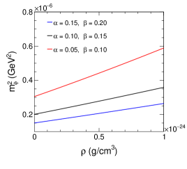
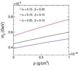
Figure 5: Relations between scalaron mass and matter density for three sets of model parameters $\alpha$ and $\beta$ after singularity correction. The left plot is for the square of the scalaron mass and the right plot is for its linear form.

Thus, after resolving this problem the scalaron can be made fairly lighter instead of extremely heavier. The cause of this attribution is seen clearly from Fig. 6 that the potential pushes the scalaron field to obtain larger values in denser environments and also, as mentioned already, the minimum of effective potential becomes shallower in the high-density region after fixing the singularity problem suffered by the model.

         

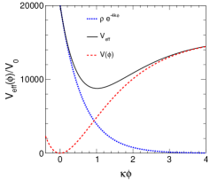
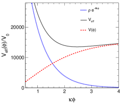
Figure 6: $R^{2}$ corrected scalaron effective potential $V_{eff}(\phi)$ (black solid line) for the considered $f(R)$ gravity model with respect to two matter distributions $\rho\sim 10^{4}\rho_{c}$ (left) and $\rho\sim 10^{5}\rho_{c}$ (right) respectively. The red dashed lines show the contributions from the original potential and the blue dotted lines represent the contributions of the density-dependent term.

In the next section, we will investigate the contribution of scalaron in modeling the alternative of dark matter in the context of galactic dynamics.

IV Rotation curves and scalaron

IV.1 Galactic rotational velocity

To derive the equation of motion of a test particle (a star) using conformal coupling we consider the motion of the particle in a static gravitational field within a constant velocity region described by the following spherically symmetric metric:

$$ds^{2}=-e^{\mu}dt^{2}+e^{\nu}dr^{2}+r^{2}d\theta^{2}+r^{2}\sin^{2}\theta\,d\varphi^{2},$$ (52)

where the metric components $\mu$ and $\nu$ are functions of the radial coordinate $r$ only. Since the conformal coupling given by equation (11) with the conformal factor expressed by equation (16) makes the interaction between scalaron field with matter distribution, we will use this coupling in the geodesic equation of the particle. On the other hand, the matter field $\psi$ couples to Jordan frame metric $g_{\mu\nu}$ instead of Einstein frame metric $\tilde{g}_{\mu\nu}$ 2018_burrage . Hence the particle follows timelike geodesic of $g_{\mu\nu}$ not that of $\tilde{g}_{\mu\nu}$. The geodesic of the particle is, therefore, given by the following equation  1992_stefan ; 2015_Zanzi :

$$\dfrac{d^{2}x^{\eta}}{d\tau^{2}}+\Gamma_{\mu\nu}^{\eta}\dfrac{dx^{\mu}}{d\tau}\dfrac{dx^{\nu}}{d\tau}=0,$$ (53)

where the Christoffel symbol (connection coefficient) which governs the motion is defined as

$$\Gamma_{\mu\nu}^{\eta}=\,\frac{1}{2}\,g^{\eta\lambda}\left[\frac{\partial g_{\mu\lambda}}{\partial x^{\nu}}+\frac{\partial g_{\nu\lambda}}{\partial x^{\mu}}-\frac{\partial g_{\mu\nu}}{\partial x^{\lambda}}\right].$$ (54)

From equations (11) and (16), we have

$$g_{\mu\nu}=e^{-\sqrt{\frac{2}{3}}\kappa\phi}\,\tilde{g}_{\mu\nu},\qquad g^{\mu\nu}=e^{\sqrt{\frac{2}{3}}\kappa\phi}\,\tilde{g}^{\mu\nu}.$$ (55)

Each term of the right-hand side of equation (54) can be replaced by respective conformally transformed equations that are obtained from equation (55). Thus, a relation between the connection coefficients in the Jordan and the Einstein frames is established 2006_Waterhouse ; 2015_Zanzi which may be written as

$$\Gamma_{\mu\nu}^{\eta}=\tilde{\Gamma}_{\mu\nu}^{\eta}-\,\frac{\kappa}{\sqrt{6}}\,\left[\frac{\partial\phi}{\partial x^{\nu}}\,\delta_{\mu}^{\eta}+\frac{\partial\phi}{\partial x^{\mu}}\,\delta_{\nu}^{\eta}-\frac{\partial\phi}{\partial x^{\lambda}}\,\tilde{g}^{\eta\lambda}\,\tilde{g}_{\mu\nu}\right].$$ (56)

Substitution of this equation in equation (54) yields

$$\dfrac{d^{2}x^{\eta}}{d\tau^{2}}+\tilde{\Gamma}_{\mu\nu}^{\eta}\dfrac{dx^{\mu}}{d\tau}\dfrac{dx^{\nu}}{d\tau}-\frac{\kappa}{\sqrt{6}}\,\left[2\,\frac{\partial\phi}{\partial x^{\mu}}\,\dfrac{dx^{\mu}}{d\tau}\,\dfrac{dx^{\eta}}{d\tau}\,-\tilde{g}^{\eta\lambda}\,\frac{\partial\phi}{\partial x^{\lambda}}\,\tilde{g}_{\mu\nu}\,\dfrac{dx^{\mu}}{d\tau}\dfrac{dx^{\nu}}{d\tau}\right]=0.$$ (57)

In the non-relativistic or weak gravity limit, the particle’s velocity is sufficiently slow, i.e. $v\ll c$ and in such a slow velocity situation the proper time $\tau$ may be approximated to the coordinate time $t$. Hence, the spatial components of four velocity $v^{i}=dx^{i}/dt\equiv\left(dx^{1}/dt,dx^{2}/dt,dx^{3}/dt\right)\ll dx^{0}/dt$ 1984_wald ; 2018_sporea . Thereby, it is seen from the above equation that the first term within the square bracket is negligible in comparison with the second term. So, in the weak field limit and for static spacetime the equation of motion contains radial component only. With the radial component of the geodesic equation, we get from equation (57) as given by

$$\dfrac{d^{2}r}{dt^{2}}=-\left[\tilde{\Gamma}_{00}^{1}-\frac{\kappa}{\sqrt{6}}\,\frac{d\phi}{dr}\right].$$ (58)

This is the equation of motion of the particle in the Einstein frame in the weak field approximation. It shows that the geodesic in this frame contains a term $\kappa/\sqrt{6}\,(d\phi/dr)$ due to the scalaron field in addition to the gravitational term. This term can be defined as the acceleration caused by chameleon force $F_{\phi}$ that appears as a result of the chameleonic nature of the scalaron field. Obviously, in the weak field limit, chameleon force exists and a test particle experiences chameleonic force apart from the gravitation force also. So, the dynamics of the test particle will be controlled by both of these two forces. Now, for simplicity, if we assume that the orbit of the particle is circular, the centripetal acceleration of the particle moving with velocity $v$ will be

$$a=-\frac{v^{2}}{r}.$$ (59)

These two equations (58) and (59) result in the following velocity equation:

$$v^{2}=r\,\left[\tilde{\Gamma}_{00}^{1}-\frac{\kappa}{\sqrt{6}}\,\frac{d\phi}{dr}\right].$$ (60)

As in the weak field limit, the velocity of a particle is vanishingly small 2014_stabile ; 2007_Capozzie as discussed before, one may obtain

$$\Gamma_{00}^{1}\simeq-\frac{1}{2}\frac{\partial g_{00}}{\partial r}.$$ (61)

Hence,

$$\tilde{\Gamma}_{00}^{1}\simeq-\frac{1}{2}\frac{\partial\tilde{g}_{00}}{\partial r}\simeq-\frac{1}{2}\frac{\partial(\Omega^{2}g_{00})}{\partial r}.$$ (62)

Next, to compute $d\phi/dr$ we will use equation (28) and the metric (52). It can be expressed as

$$\frac{d\phi}{dr}=\frac{d\phi}{dR}\frac{dR}{dr}.$$ (63)

From the metric (52) Ricci scalar is obtained as

$$R=\frac{e^{-\nu}}{2r^{2}}\Big{[}-4+4e^{\nu}-r^{2}\mu^{\prime 2}+4r\nu^{\prime}+r\mu^{\prime}(-\,4+r\nu^{\prime})-2r^{2}\mu^{\prime\prime}\ \Big{]},$$ (64)

where the prime denotes the derivative with respect to the radial coordinate $r$. Thus

$$\dfrac{dR}{dr}=\frac{e^{-\nu}}{2r^{3}}\Big{[}8-8e^{\nu}+r^{3}\mu^{\prime 2}\nu+r\mu^{\prime}\big{\{}4 +r(4\nu^{\prime}-r\nu^{2}+r(-\,2\mu^{\prime\prime}+\nu^{\prime\prime}))\big{\}}\,+$$

$$r^{2} (-\,4\nu^{\prime 2}-4\mu^{\prime\prime}+3r\nu^{\prime}\mu^{\prime\prime}+4\nu^{\prime\prime}-2r\mu^{\prime\prime\prime})\Big{]}.$$ (65)

It is clear from equations (62) and (65) that to have a precise velocity equation from equation (60), we need to derive the explicit forms of the $e^{\mu}$ and $e^{\nu}$ first. These coefficients will shape the velocity profile of the particle by determining $dR/dr$ and $\Gamma_{00}^{1}$ respectively.

In the said context, it is worth mentioning that the generalized field equation of an MTG can be recast in the form given below  2023_Nashiba ; 2018_sporea ; 2015_mimoso ; 2016_Wojnar :

$$\xi(\varphi)\left[G_{\mu\nu}+X_{\mu\nu}\right]=\kappa^{2}\,T_{\mu\nu},$$ (66)

where $X_{\mu\nu}$ is an additional term that appeared due to modification of geometry in an MTG, $\xi(\varphi)$ is a coupling factor that couples geometry to matter, $\varphi$ may be a curvature invariant or other gravitational field such as a scalar field. For $X_{\mu\nu}=0$ and $\xi(\varphi)=1$, one can recover GR. In our case, we have equation (7) similar to generalized equation (66), where the coupling factor $\xi(\varphi)=f_{R}$ and the tensor $G_{\mu\nu}^{d}$ represents the modified term regarding GR. From the metric (52) and the generalized field equation (66), derivation of the metric coefficient $e^{\nu}$ is accomplished in Refs. 2023_Nashiba and is found as

$$e^{\nu}=\left(1-\frac{2G\bar{M}(r)}{r}\right)^{-1}=\left(1-\frac{2GM(r)}{\Omega^{2}\,r}\right)^{-1}\!\!\!\!,$$ (67)

where $\bar{M}(r)$ denotes modified mass profile which is

$$\bar{M}(r)=\frac{M(r)}{\Omega^{2}}=\frac{1}{\Omega^{2}}\int_{0}^{r}\left(\frac{\kappa^{2}\rho\,r^{2}}{2Gf_{R}(r)}-\Omega^{2}\,\frac{r^{2}X_{00}(r)}{2Ge^{\mu}}\right)dr.$$ (68)

Equation (67) indicates the resemblance of the form of metric coefficient $e^{\nu}$ to the standard Schrawzchild form. As in the limit $r\rightarrow\infty$, i.e. at very large distance from the source of the gravitation field (in our case from the center of the galaxy), the metric coefficients can plausibly be assumed in the standard Schrawzchild form. Therefore, we consider the weak field limit where the spacetime can be adopted as Minkowskian and thereby can be expressed $\tilde{g}_{\mu\nu}$ in terms of Minkowski metric $\eta_{\mu\nu}$ as  1992_stefan ; 2023_Nashiba

$$\tilde{g}_{\mu\nu}=\Omega^{2}\left(\eta_{\mu\nu}+g_{\mu\nu}\right),$$ (69)

and we obtain $g_{00}=-\,2\phi$ to the first order in $g_{\mu\nu}$, where $\phi=GM_{1}(r)/r=GM(r)/\Omega^{2}r$. Hence, we may write $e^{\mu}$ from equation (69) as

$$e^{\mu}\approx 1-\frac{2G\bar{M}(r)}{r}=1-\frac{2GM(r)}{\Omega^{2}\,r}.$$ (70)

Thus, $\tilde{\Gamma}_{00}^{1}$ of equation (62) takes the form:

$$\tilde{\Gamma}_{00}^{1}=\frac{GM(r)}{r^{2}}.$$ (71)

On the other hand, we require derivatives of metric functions to get $dR/dr$ exactly. On that account, the metric functions are written from (67) and (70) as

$$\nu(r) =\ln\left(1-\frac{2GM(r)}{\Omega^{2}\,r}\right)^{-1}\!\!\!\!\!,$$ (72)

$$\mu(r) =\ln\left(1-\frac{2GM(r)}{\Omega^{2}\,r}\right).$$ (73)

After performing derivations of these two equations with respect to $r$ we are able to find

$$\nu^{\prime} =-\left(\frac{2M(r)}{\Omega^{2}\,r^{2}}-\frac{4M^{2}(r)}{\Omega^{4}\,r^{3}}\right)e^{2\nu},\;\;\;\nu^{\prime\prime}=\frac{4M(r)}{\Omega^{2}\,r^{3}}e^{\nu}+\frac{4M^{2}(r)}{\Omega^{4}\,r^{4}}e^{2\nu}.$$ (74)

$$\mu^{\prime} =\frac{2M(r)}{\Omega^{2}\,r^{2}}e^{\nu},\;\;\;\mu^{\prime\prime}=-\frac{4M(r)}{\Omega^{2}\,r^{3}}e^{\nu}-\frac{4M^{2}(r)}{\Omega^{4}\,r^{4}}e^{2\nu},$$ (75)

$$\mu^{\prime\prime\prime} =\frac{24M^{2}(r)}{\Omega^{4}\,r^{5}}e^{2\nu}+\frac{12M(r)e^{\nu}}{\Omega^{2}\,r^{4}}+\frac{16M^{3}(r)}{\Omega^{6}\,r^{6}}e^{3\nu}.$$ (76)

On substitution of equations (67), (72) and (74) – (76) into equation (65) we attain the expression of $d\phi/dr$ from equation (63) with the help of equation (28) after being carried out some algebraic calculations as given by

$$\frac{d\phi}{dr}=\frac{2\sqrt{6}f_{RR}}{r^{3}\kappa f_{R}}\left[-1+e^{-\nu}-\frac{2M^{3}(r)}{\Omega^{6}\,r^{3}}e^{2\nu}-\frac{3M^{2}(r)}{\Omega^{4}\,r^{2}}e^{\nu}+\frac{3M^{2}(r)}{\Omega^{4}\,r^{3}}e^{\nu}+\frac{2M^{3}(r)}{\Omega^{6}\,r^{4}}e^{\nu}+\frac{4M}{\Omega^{2}r}\right].$$ (77)

Our purpose is to find the rotational velocity of a particle (star) according to equation (60). This is the equation of motion of a particle that follows the geodesic of metric $g_{\mu\nu}$ basically under the static and weak field approximation of the gravitation field sourced by a galaxy. Thus, we obtain the rotational velocity equation for the particle by inserting equations (71) and (77) into equation (60), and also writing $\Omega^{2}=f_{R}$ as follows:

$$v^{2}=\frac{GM(r)}{r}+\frac{2f_{RR}}{r^{2}f_{R}}\left[1-e^{-\nu}+\frac{2M^{3}(r)}{f_{R}^{3}\,r^{3}}e^{2\nu}+\frac{3M^{2}(r)}{f_{R}^{2}\,r^{2}}e^{\nu}-\frac{3M^{2}(r)}{f_{R}^{2}\,r^{3}}e^{\nu}-\frac{2M^{3}(r)}{f_{R}^{3}\,r^{4}}e^{\nu}-\frac{4M}{rf_{R}}\right].$$ (78)

However, in our work instead of complex mass distribution illustrated by equation (66), we assume a simple distribution of mass in a galaxy represented by the mass model 2018_sporea :

$$M(r)=M_{0}\left[\sqrt{\frac{r_{0}}{r_{c}}}\left(\frac{r}{r+r_{c}}\right)\right]^{3b}\!\!\!\!,$$ (79)

where $r_{0}$ is a scale length, $M_{0}$ and $r_{c}$ are the total mass and core radius of the galaxy respectively. The value of the parameter $b$ is $1$ for HSB and it is $2$ for both LSB and Dwarf galaxies. It should be mentioned that values of $M_{0}$ and $r_{c}$ have to be estimated from the fitting of theoretical rotation curves with observations of respective galaxies.

Table 1: Different physical properties of a set of fifteen observed LSB galaxies and the best-fitted values of total mass $M_{0}$ and core radius $r_{c}$ of each galaxy for the $f(R)$ gravity model (33).

Galaxy Name	Scale length	Distance $D$	Luminosity $L_{B}$	Mass $M_{0}$	Core Radius	$\chi^{2}_{red}$
	$r_{0}$ (kpc)	(Mpc)	($10^{10}L_{\odot}$)	($10^{10}M_{\odot}$)	$r_{c}$ (kpc)
DDO 064	0.69	6.8	0.015	4.1	2.04	0.53
F563-V2	2.43	59.7	0.266	2.00	1.50	2.20
F 568-3	4.99	82.4	0.351	1.20	2.50	0.42
F 583-1	2.36	35.4	0.064	4.10	2.16	0.39
F 583-4	1.93	53.3	0.096	0.50	1.23	0.33
NGC 300	1.75	2.08	0.271	3.30	1.54	1.50
NGC 2976	1.01	3.58	0.201	1.01	0.84	0.92
NGC 3109	1.56	1.33	0.064	1.50	1.45	1.50
NGC 3917	2.63	18.0	1.334	8.00	2.15	5.10
NGC 4010	2.81	18.0	0.883	4.10	2.00	0.20
NGC 1003	1.61	11.4	1.480	5.60	1.80	0.09
UGC 5750	3.46	58.7	0.472	9.60	3.56	0.31
UGC 6983	3.21	18.0	0.577	1.80	1.90	1.50
UGC 7089	2.26	18.0	0.352	11.6	2.70	0.24
UGC 11557	2.75	24.2	1.806	3.10	2.20	0.59

Table 2: Different physical properties of a set of ten observed HSB galaxies and the best-fitted values of total mass $M_{0}$ and core radius $r_{c}$ of each galaxy for the $f(R)$ gravity model (33).

Galaxy Name	Scale length	Distance $D$	Luminosity $L_{B}$	Mass $M_{0}$	Core Radius	$\chi^{2}_{red}$
	$r_{0}$ (kpc)	(Mpc)	($10^{10}L_{\odot})$	($10^{10}M_{\odot}$)	$r_{c}$ (kpc)
NGC 2903	2.33	6.6	4.088	23.00	2.50	4.50
NGC 2998	6.20	68.1	5.186	16.00	3.90	1.04
NGC 3198	3.14	13.8	3.241	102.50	6.70	1.20
NGC 3769	3.38	18.0	0.684	22.80	4.90	0.12
NGC 4088	2.58	18.0	2.957	69.40	5.00	0.62
NGC 4157	2.32	18.0	2.901	81.60	4.46	1.91
NGC 4183	2.79	18.0	1.042	29.00	5.25	1.70
NGC 4217	2.94	18.0	3.031	57.20	4.70	0.71
NGC 5055	3.20	9.9	3.622	56.00	4.50	0.41
NGC 7793	1.21	3.61	0.910	20.00	2.80	3.06

Table 3: Different physical properties of a set of twelve observed dwarf galaxies and the best-fitted values of total mass $M_{0}$ and core radius $r_{c}$ of each galaxy for the $f(R)$ gravity model (33).

Galaxy Name	Scale length	Distance ($D$)	Luminosity ($L_{B})$	Mass ($M_{0}$)	Core Radius	$\chi^{2}_{red}$
	$r_{0}$ (kpc)	(Mpc)	$10^{10}L_{\odot}$	$10^{10}M_{\odot}$	$r_{c}$ (kpc)
NGC 2366	0.65	3.27	0.236	5.44	1.10	5.04
NGC 3877	2.53	18.0	1.948	6.00	1.72	4.60
NGC 3972	2.18	18.0	0.978	7.40	1.85	1.20
NGC 5585	1.53	7.06	0.333	5.40	1.60	4.90
UGC 4325	1.86	9.6	2.026	0.25	0.84	7.10
UGC 4499	1.73	12.5	1.552	1.40	1.38	2.01
UGC 6446	1.49	12.0	0.988	2.00	1.28	0.54
UGC 6667	5.15	18.0	0.422	0.13	1.60	2.20
UGC 6818	1.39	18.0	0.352	9.00	1.90	0.96
UGC 6917	2.76	18.0	6.832	0.92	1.50	1.20
UGC 7524	3.46	4.74	2.436	0.90	2.00	0.77
UGC 12632	2.42	9.77	1.301	1.06	1.68	0.70

       

       

       

       

       

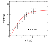
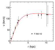
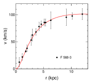
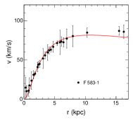
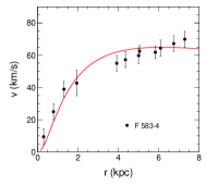
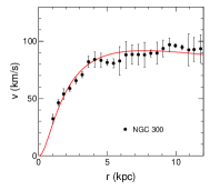
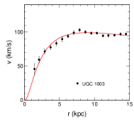
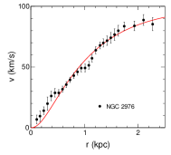
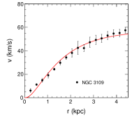
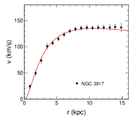
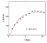
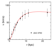
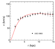
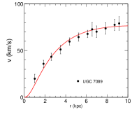
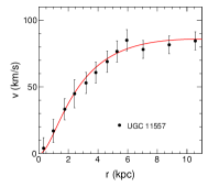
Figure 7: Fitting of rotation curves generated from the $f(R)$ gravity model (33) for rotation velocities of a sample of 15 galaxies with their quoted errors. The data points are observational values of rotational velocities extracted from Ref. 2016_Lelli .

IV.2 Fitting of rotation curves and estimation of parameters

The rotational velocity of a particle rotating around the galactic center have been derived in the last subsection based on a recently introduced new $f(R)$ gravity model (33). We generate rotation curves for the test particle according to equation (78) and intend to examine the influence of scalaron on rotational profiles to explain galactic dynamics in the absence of dark matter by fitting the theoretically predicted curves with the observational data of a sample of 37 galaxies including fifteen LSB, ten HSB and twelve dwarf galaxies 2016_Lelli .

       

       

       

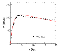
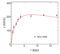
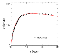
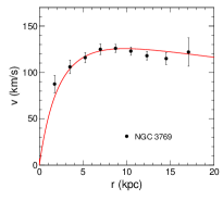
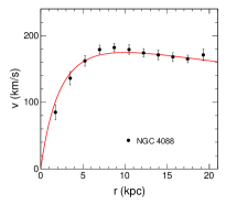
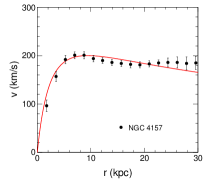
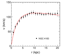
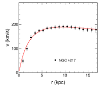
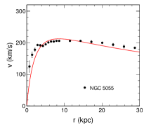
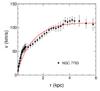
Figure 8: Fitting of rotation curves generated from the $f(R)$ gravity model (33) for rotation velocities of a sample of 10 HSB galaxies with their quoted errors. The data points are observational values of rotational velocities extracted from Ref. 2016_Lelli .

It is noteworthy that LSB galaxies are slowly evolving objects that have DM domination in all radii. They live in less dense, extremely extended DM halos and are found to be more isolated relative to HSB galaxies 1997_Bothun ; 1997_Blok . Refs. 2002_blok ; 1996_blok ; 2017_Karukes have analyzed that the rotation curves of LSB and Dwarf galaxies are slowly rising, shallower at small radii. Contrary to this, an HSB galaxy has a higher central mass density that leads to a steeply rising rotation curve in the inner region followed by a relatively flat outer part 2014_McGaugh . Taking note of these results, rotation curves for all these three types of galaxies are produced and fitted by considering a predetermined set of model parameters $\alpha=0.0005$ and $R/R_{c}=2$ from Ref. 2020_dhruba for all the samples. Also, another model parameter $\beta$ is set to $0.0001$ for each galaxy, and fitting of theoretical curves is carried out by constraining parameters $M_{0}$ and $r_{c}$ using the best-fitted values for each sample galaxy. A notable agreement between predictions and actual observations is observed for all samples. These perfectly matched rotation curves with observational data, extracted from Ref. 2016_Lelli , estimate the values of $M_{0}$ and $r_{c}$ well and are obtained as per the characteristics of different classes of galaxies. The LSB galaxies can be fitted from a maximum radial distance $2.5$ kpc to $22.5$ kpc. Similarly, HSB galaxies’ maximum fitted radial distance varies from $6$ kpc to $30$ kpc and in the case of dwarf galaxies it is from $6$ kpc to $12$ kpc. In Tables 1, 2 and 3, the successfully fitted values of $M_{0}$ and $r_{c}$ are listed together with some other galactic parameters extracted from Ref. 2012_mann and reduced $\chi^{2}$ values of fitting for different galaxies. From the tables, it is seen that for HSB galaxies total mass $M_{0}$, in the solar mass unit (here we consider $M_{0}=10^{10}M_{\odot}$), is large and in the case of LSB and dwarf galaxies this value is small.

The behavior of galactic rotation curves of 37 sample galaxies are presented in Figs. 7, 8 and 9 respectively. Furthermore, we are endeavoring to understand the effectiveness of the chameleon field on the dynamics of galaxies. For this purpose, we plot the difference between the velocity determined by equation (78) and the Newtonian velocity $GM(r)/r$ as a function of radial distance $r$ for 6 sample galaxies taking two from each category LSB, HSB and Dwarf (see Fig. 10) utilizing the values of model parameters that have already been taken into account and the same values of $M_{0}$ and $r_{c}$ obtained from Tables 1, 2 and 3 of respective galaxies. It is observed from Fig. 10 that the difference between these two velocities is not noticeably large. This result suggests a marginal impact of the chameleon field on galactic rotation curves. Thus, the behavior of rotation curves through modification of gravity by a scalar field attributing chameleonic nature can be illustrated using the newly introduced $f(\mathcal{R})$ model.

       

       

       

       

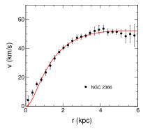
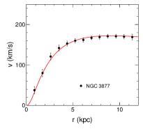
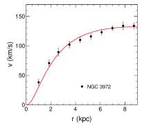
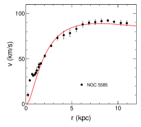
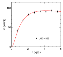
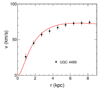
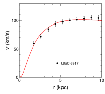
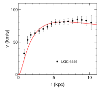
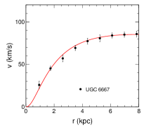
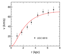
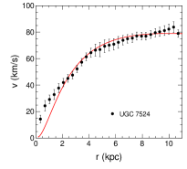
Figure 9: Fitting of rotation curves generated from the $f(R)$ gravity model (33) for rotation velocities of a sample of 12 dwarf galaxies with their quoted errors. The data points are observational values of rotational velocities extracted from Ref. 2016_Lelli .

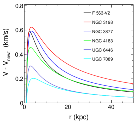
Figure 10: Difference of velocity $V$ and Newtonian velocity $V_{newt}$ i.e., $(V-V_{newt})$ against radial distance $r$. $V$ is derived from equation (78) and $v_{newt}=GM(r)/r.$

V Conclusions

The DM issue is one of the greatest theoretical difficulties in modern physics in general and astrophysics in particular. Usually, the unique behavior of galactic rotation curves is interpreted by postulating the existence of this invisible matter distributed in a spherical halo around the galaxies. Of course, lack of acceptable evidences of such matter, modification of gravity is considered as a reasonable alternative for the explanation of observed galactic rotation curves. Looking into this, we thought about a popular and one of the simplest MTGs, the $f(R)$ gravity, for our study. Using the metric formalism of the theory we have derived the field equations first and then obtained the equation for the extra degree of freedom $f_{R}$ by taking the trace of the field equation.

To identify the extra degree of freedom $f_{R}$ as a scalar field (scalaron), we used a frame transformation called conformal or Weyl transformation that provides coupling of the scalaron with matter minimally. This minimal coupling simplifies the field equation of $f(R)$ theory of gravity in the Einstein frame rather than the Jordan frame. It is observed that the scalaron field potential in this case plays a significant role and results in the local matter density-dependent effective field mass giving the field a chameleonic character. Then by adopting a recently introduced $f(R)$ model, we tried to check the viability of the model regarding the chameleonic nature shown by the scalaron. Also, the singularity problem suffered by the model is discussed and resolved it.

We aimed to investigate the effect of scalaron on the rotation curves of galaxies. For this, by considering a star as a test particle in a static spherically symmetric spacetime we have derived the rotation velocity equation of the particle with a contribution from the scalaron field in the Einstein frame and generated rotation curves of 37 samples of galaxies. Total mass $M_{0}$ and the core radius $r_{c}$ are determined for each galaxy from the fitting of predicted rotation curves to observed data of the sample galaxies by employing the $\chi^{2}$ minimization technique. The $\chi^{2}_{red}$ values are displayed in respective tables against each galaxy. It is seen that the $\chi^{2}_{red}$ values are not equivalent or close to $1$ relative to all the galaxies. In case of galaxies NGC2366, NGC2903, NGC7793, UGC4325, NGC3877 and NGC5585, its value is quite larger than $1$. Still, we can almost fit the curves successfully where the predicted curves exhibit a nice and good agreement with the observed curves as shown in respective figures. Moreover, in order to comprehend the extent of the impact of scalaron, we have depicted velocity difference curves of $6$ galaxies two each from the LSB, HSB and dwarf with respect to radial distance $r$ for similar values of model parameters $\alpha$, $\beta$ and of $M_{0}$ and $r_{c}$ estimated by the best-fitted curves of respective galaxies.

Hence, we can conclude that any explicit form of dark matter may not be necessary for exploring galactic dynamics by means of chameleon $f(R)$ gravity. However, in contrast to the approach centered on the single mass model, there are possibilities for comparative study by considering different mass profiles derived from the density distributions such as Navarro-Frenk-White (NFW), pseudo-isothermal (ISO) 1997_nava ; 2013_sofue ; 2008_block etc. with other convenient modified gravity models. We aim to develop the work further sustaining this viewpoint in the future.

References

- (1) V. C. Rubin and W. K. Ford, Rotation of the Andromeda Nebula from a Spectroscopic Survey of Emission Regions, ApJ 159, 379 (1970).
- (2) V. C. Rubin, W. K. Ford and N. Thonnard, Extended Rotation Curves of High-Luminosity Spiral Galaxies. IV. Systematic Dynamical Properties, SaSc, ApJ 225, L107 (1978).
- (3) V. C. Rubin, The Rotation of Spiral Galaxies, Science 220, 4604 (1983).
- (4) K. Garrett and G. Duda, Dark Matter: A Primer, Adv. Astron. 2011, 968283 (2011) [arXiv:1006.2483].
- (5) R. Massey, T. Kitching and J. Richard, The dark matter of gravitational lensing, Rep. Prog. Phys. 73, 086901 (2010) [arXiv:1001.1739].
- (6) S. Shankaranarayanan and J. P. Johnson, Modified theories of Gravity: Why, How and What?, Gen. Rel. & Grav. 54, 44 (2022) [arXiv:2204.06533].
- (7) M. Milgrom, A modification of the Newtonian dynamics as a possible alternative to the hidden mass hypothesis, ApJ 270, 365 (1983).
- (8) T. Harko and F. S. N. Lobo, f(R,) gravity, Eur. Phys. J. C 70, 373 (2010) [arXiv:1008.4193v2].
- (9) T. Harko, F. S. N. Lobo, S. Nojri, S. D. Odintsov, f(R,T) gravity, Phys. Rev. D 84, 024020 (2011) [arXiv:1104.2669].
- (10) S. Capozziello and M. Francaviglia, Extended Theories of Gravity and their Cosmological and Astrophysical Applications, Gen. Rel. & Grav. 40, 357 (2008) [arXiv:0706.1146].
- (11) S. Capozziello and M. De Laurentis, Extended Theories of Gravity, Phys. Rep. 509, 167 (2011) [arXiv:1108.6266].
- (12) L. Atayde and N. Frusciante, Can f(Q) gravity challenge CDM ?, Phys. Rev. D 104, 064052 (2021) [arXiv:2108.10832v2].
- (13) Y. Sobouti, An f(R) gravitation for galactic environments, A&A 464, 921 (2007) [arXiv:astro-ph/0603302].
- (14) C. G. Böhmer, T. Harko, F. S. N. Lobo, Dark matter as a geometric effect in f(R) gravity, Astropart. Phys. 29, 386 (2008)[arXiv:0709.0046].
- (15) T. Harko, Galactic rotation curves in modified gravity with non-minimal coupling between matter and geometry, Phys. Rev. D 81, 084050 (2010) [arXiv:1004.0576].
- (16) L. Á. Gegurgel et al, Galactic rotation curves in brane world models, MNRAS 415 3275, (2011) [arXiv:1105.0159].
- (17) R. Zaregonbadi, M. Farhoudi and N. Riazi, Dark matter from f(R,T) gravity, Phys. Rev. D 94, 084052 (2016) [arXiv:1608.00469].
- (18) A. Finch and J. L. Said, Galactic rotation dynamics in gravity, Eur. Phys. J. C 78, 560 (2018) [arXiv:1806.09677].
- (19) N. Parbin and U. D. Goswami, Scalarons mimicking Dark Matter in the Hu-Sawicki model of f(R) gravity, Mod. Phys. Lett. A 36, 2150265 (2021) [arXiv:2007.07480].
- (20) N. Parbin and U. D. Goswami, Galactic rotation dynamics in a new f(R) gravity model, Eur. Phys. J. C 83, 411 (2023) [arXiv:2208.06564v2].
- (21) H. Shabani and P. H. R. S. Moraes, Galaxy rotation curves in the f(R,T) gravity formalism, Phys. Scr. 98, 065302 (2023) [arXiv:2206.14920].
- (22) S. Chakraborty, An alternative f(R,T) gravity theory and the dark energy problem, Gen. Rel. & Grav. 45, 2052 (2013) [arXiv:1212.3050].
- (23) S. Capozziello, V. F. Cardone, and A. Troisi, Dark energy and dark matter as curvature effects, JCAP 0608, 001, (2006) [arXiv:astro-ph/0602349].
- (24) A. Joyce, L. Lombriser and F. Schmidt, Dark Energy Versus Modified Gravity, Ann. Rev. Nucl. & Part. Sci. 66, 95 (2016) [arXiv:1601.06133].
- (25) P. J. E. Peebles and B. Ratra, The cosmological constant and dark energy, Rev. Mod. Phys. 75, 559 (2002) [arXiv:astro-ph/0207347].
- (26) H. A. Buchdahl, Non-Linear Lagrangians and Cosmological Theory, MNRAS 150, 1 (1970).
- (27) A. A. Starobinski, A new type of isotropic cosmological models without singularity, Phys. Lett. B 91, 99 (1980).
- (28) D. J. Gogoi and U. D. Goswami, A new f(R) Gravity Model and properties of Gravitational Waves in it, Eur. Phys. J. C 80, 1101 (2020) [arXiv:2006.04011v2].
- (29) W. Hu and I. Sawicki, Models of f(R) cosmic acceleration that evade solar system tests, Phys. Rev. D 76, 064004 (2007) [arXiv:0705.1158].
- (30) F. G. Alvarenga, M. J. S. Houndjo, A. V. Monwanou and J. B. C. Orou, Testing some f(R,T) gravity models from energy conditions, J. Mod. Phys., 4, 130 (2013) [arXiv:1205.4678].
- (31) D. Lovelock, The Einstein tensor and its generalizations, J. Math. Phys. 12, 498 (1971).
- (32) S. Nojiri and S. D. Odintsov, Modified Gauss-Bonnet theory as gravitational alternative for dark energy, Phys. Lett. B 631, 1 (2005) [arXiv:hep-th/0508049].
- (33) T. Chiba, 1/R gravity and Scalar-Tensor Gravity, Phys. Lett. B 575, 1 (2003) [arXiv:astro-ph/0307338].
- (34) M. Kunz and D. Sapone, Dark Energy versus Modified Gravity, Phys. Rev. Lett. 98, 121301 (2007) [arXiv:astro-ph/0612452].
- (35) S. Shahidi and H. R. Sepangi, Brane worlds and dark matter, IJMP D 20, 77 (2011) [arXiv:1009.5458].
- (36) A. D. Felice and S. Tsujikawa, f(R) theories, Liv. Rev. Rel. 13, 3 (2010) [arXiv:1002.4928].
- (37) T. Faulkner, M. Tegmark, E. F. Bunn and Y. Mao, Constraining f(R) Gravity as a Scalar Tensor Theory, Phys. Rev. D 76, 063505 (2006) [arXiv:astro-ph/0612569].
- (38) T. Tamaki, S. Tsujikawa, Revisiting chameleon gravity-thin-shells and no-shells with appropriate boundary conditions, Phys. Rev. D 78, 084028 (2008) [arXiv:0808.2284].
- (39) T. Cliftone, P. G. Ferreira, A. Padilla and C. Skordis, Modified Gravity and Cosmology, Phys. Rep. 1, 513 (2012) [arXiv:1106.2476].
- (40) A. Joyce, B. Jain, J. Khoury and M. Trodden, Beyond the Cosmological Standard Model, Phys. Rep. 568, 1 (2015) [arXiv:1407.0059].
- (41) A. Terukina, et al, Testing chameleon gravity with the Coma cluster, JCAP 04, 013 (2014) [arXiv:1312.5083].
- (42) K. Koyama, Cosmological tests of modified gravity, Rep. Prog. Phys. 79, 046902 (2016) [arXiv:1504.04623].
- (43) C. Burrage and J. Sakstein, Tests of Chameleon Gravity, Liv. Rev. Rel. 1, 21 (2018) [arXiv:1709.09071].
- (44) T. Chiba, T. L. Smith and A. L. Erickcek, Solar System constraints to general f(R) gravity, Phys. Rev. D 75, 124014 (2007) [arXiv:astro-ph/0611867].
- (45) J. Khoury and A. Weltman, Chameleon cosmology, Phys. Rev. D 69, 044026 (2004) [arXiv:astro-ph/0309411].
- (46) J. Khoury and A. Weltman, Chameleon Fields:Awaiting Surprises for Tests of Gravity in Space, Phys. Rev. Lett. 93, 17110 (2004) [arXiv:astro-ph/0309300].
- (47) J. Khoury, Chameleon Field Theories, Class. Quant. Grav. 30, 214004 (2013) [arXiv:1306.4326].
- (48) K. Hinterbichler and J. Khoury, Symmetron Fields:Screening Long-Range Forces Through Local Symmetry Restoration, Phys. Rev. Lett. 104, 231301 (2010) [arXiv:1001.4525].
- (49) M. M. Verma and B. K. Yadav, Observational Role of Dark Matter in f(R) Models for Structure Formation, IJMP: Conf. Ss. 46, 1860045 (2018).
- (50) T. Katsuragawa and S. Matsuzaki, Modified Gravity Explains Dark Matter?, Phys. Rev. D 95, 044040 (2017) [arXiv:1610.01016].
- (51) T. Katsuragawa and S. Matsuzaki, Cosmic History of Chameleonic Dark Matter in F(R) Gravity, Phys. Rev. D 97, 064037 (2018) [arXiv:1708.08702].
- (52) P. Burikham and S. Panpanich, Effects of Chameleon Scalar Field on rotation curves of the galaxies, IJMP D 21, 1250041 (2012) [arXiv:1103.1198].
- (53) P. D. Mannheim and J. G. O’Brien, Fitting galactic rotation curves with conformal gravity and a global quadratic potential, Phys. Rev. D 85, 124020 (2012) [arXiv:1011.3495].
- (54) Y. Shtanov, Light scalaron as dark matter, Phys. Lett. B 820, 136469 (2021) [arXiv:2105.02662].
- (55) A. P. Naik, E. Puchwein, A. C. Davis and C. Arnold, Imprints of Chameleon f(R) gravity on Galaxy rotation curves, MNRAS 480, 5211 (2018) [arXiv:1805.12221].
- (56) Q. Li and L. Modesto, Galactic Rotation Curves in Conformal Scalar-Tensor Gravity, Grav. & Cos. 26, 99 (2020).
- (57) J. R. Brownstein1 and J. W. Moffat, Galaxy Rotation Curves without Nonbaryonic Dark Matter, ApJ 636, 721 (2006) [arXiv:astro-ph/0506370].
- (58) D. J. Gogoi and U. D. Goswami, Cosmology with a new f(R) gravity model in Palatini formalism, IJMP D 31, 2250048 (2022) [arXiv:2108.01409].
- (59) T. P. Sotiriou and V. Faraoni, f(R) Theories of Gravity, Rev. Mod. Phys. 82, 451 (2010) [arXiv:0805.1726].
- (60) B. Li, G. B. Zhao and K. Koyama, Halos and Voids in f(R) Gravity, MNRAS 421, 3481 (2012) [arXiv:1111.2602v1].
- (61) B. Whitt, Fourth Order Gravity as General Relativity Plus Matter Phys. Lett. B 145, 176 (1984).
- (62) J. Velásquez and L. Castañeda, Equivalence between Scalar-Tensor theories and-gravity: From the action to Cosmological Perturbations J. Phys. Com. 4, 055007 (2020) [arXiv:1808.05615].
- (63) V. Faraoni and S. Nadeau, The (pseudo)issue of the conformal frame revisited, Phys. Rev. D 75, 023501 (2007) [arXiv:gr-qc/0612075].
- (64) C. A. Sporea, Notes on f(R) Theories of Gravity, (2014) [arXiv:1403.3852].
- (65) M. P. Dabrowski, J. Garecki, D. B. Blaschke, Conformal transformations and conformal invariance in gravitation, Ann. Phys. (Berlin) 18, 13 (2009) [arXiv:0806.2683v3].
- (66) V. Faraoni and E. Gunzig, Einstein frame or Jordan frame? IJTP. 38, 217 (1999) [arXiv:astro-ph/9910176].
- (67) U. D. Goswami and K. Deka, Cosmological dynamics of f(R) gravity scalar degree of freedom in Einstein frame, IJMP D, 22, 1350083 (2013) [arXiv:1303.5868v2].
- (68) A. V. Frolov, A Singularity Problem with f(R) Dark Energy Phys. Rev. Lett. 101, 061103 (2008) [arXiv:0803.2500].
- (69) T. Kobayashi and K. Maeda, Can higher curvature corrections cure the singularity problem in f(R) gravity? Phys. Rev. D 79, 024009 (2009) [arXiv:0810.5664].
- (70) S. Weinberg, Gravitation and Cosmology Principles and Applications of the General Theory of Relativity, John Wiley Sons, New York, (1972).
- (71) A. Zanzi, Chameleonic Theories: A Short Review, Universe 1(3), 446 (2015) [arXiv:1602.03869].
- (72) T. P. Waterhouse, An Introduction to Chameleon Gravity, (2006) [arXiv:astro-ph/0611816].
- (73) R. Wald, General Relativity, The University of Chicago Press, Chicago and London, pp 77 (1984).
- (74) C. A. Sporea, A. Borowiec and A. Wojnar, Galaxy Rotation Curves via Conformal Factors, Eur. Phys. J. C 78, 308 (2018) [arXiv:1705.04131].
- (75) A. Stabile and S. Capozziello, Self-gravitating systems in Extended Gravity, Galaxies, 2(4), 520 (2014) [arXiv:1411.3143].
- (76) S. Capozziello, A. Stabile and A. Troisi, The Newtonian Limit of F(R) gravity, Phys. Rev. D 76, 104019 (2007) [arXiv:0708.0723].
- (77) J. P. Mimoso, F. S. N. Lobo and S. Capozziello, Extended Theories of Gravity with Generalized Energy Conditions, J. Phys: Conf. Ss. 600, 012047 (2015) [arXiv:1412.6670].
- (78) A. Wojnar and H. Velten, Equilibrium and stability of relativistic stars in extended theories of gravity, Eur. Phys. J. C 76, 697 (2016) [arXiv:1604.04257].
- (79) F. Lelli, S. S. McGaugh and J. M. Schombert, SPARC: Mass Models for 175 Disk Galaxies with Spitzer Photometry and Accurate Rotation Curves, AJ 152, 157 (2016) [arXiv:1606.09251]; http://adsabs.harvard.edu/abs/2016arXiv160609251L.
- (80) G. Bothun, C. Impey and S. McGaugh, Low-Surface-Brightness Galaxies: Hidden Galaxies Revealed, PASP 109, 745 (1997).
- (81) W. J. G. de Blok and S. S. Mcgaugh, The dark and visible matter content of low surface brightness disc galaxies, MNRAS 290, 533 (1997).
- (82) W. J. G. de Blok and A. Bosma, High-resolution rotation curves of low surface brightness galaxies, A&A. 385, 816 (2002) [arXiv:astro-ph/0201276].
- (83) W. J. G. de Blok and S. S. McGaugh, Does low surface brightness mean low surface density?, ApJ 469, L89 (1996) [arXiv:astro-ph/9607042].
- (84) E. V. Karukes and P. Salucci, The universal rotation curve of dwarf disk galaxies, MNRAS 465, 4703 (2017) [arXiv:1609.06903].
- (85) S. S. McGaugh, The Third Law of Galactic Rotation, Galaxies 2(4), 601 (2014) [arXiv:1412.3767].
- (86) J. F. Navarro, C. S. Frenk and S. D. M. White, A Universal Density Profile from Hierarchical Clustering, ApJ 490, 493 (1997) [arXiv:astro-ph/9611107].
- (87) Y. Sofue, The Mass Distribution and Rotation Curve in the Galaxy, Plts, Strs. & Str. Systs. 985, (2013) [arXiv:1307.8215].
- (88) W. J. G. de Blok et al, High-Resolution Rotation Curves and Galaxy Mass Models from THINGS, AJ 136, 2648 (2008) [arXiv:0810.2100].