GPU-accelerated nonlinear model predictive control with ExaModels and MadNLP

Abstract

We investigate the potential of Graphics Processing Units (GPUs) to solve large-scale nonlinear model predictive control (NMPC) problems. We accelerate the solution of the constrained nonlinear programs in the NMPC algorithm using the GPU-accelerated automatic differentiation tool ExaModels with the interior-point solver MadNLP. The sparse linear systems formulated in the interior-point method is solved on the GPU using a hybrid solver combining an iterative method with a sparse Cholesky factorization, which harness the newly released NVIDIA cuDSS solver. Our results on the classical distillation column instance show that despite a significant pre-processing time, the hybrid solver allows to reduce the time per iteration by a factor of 25 for the largest instance.

I INTRODUCTION

Model predictive control (MPC) has become a standard control paradigm for physical systems with operational constraints. While classical MPC considers only quadratic costs and linear dynamics, nonlinear MPC (NMPC) looks instead at dynamic problems with nonlinear costs, dynamics, and algebraic constraints [1]. With its flexible formalism, NMPC is used in fields as diverse as process engineering or robotics [2].

Model predictive control methods make control decisions by solving optimal control problems in real time. Once the problem is formulated, the solution of optimal control problems is delegated to a nonlinear optimization solver. It is well known that for problems with a dynamic structure, the Newton step is equivalent to a linear-quadratic problem, solvable using dynamic programming recursion or the Riccati equations [3]. By doing so, the method exploits the dynamic structure explicitly. Alternatively, one can leverage the structure implicitly inside a sparse direct solver, in charge of finding an appropriate ordering to reduce the fill-in in the sparse factorization [4]. That kind of many-degrees-of-freedom approaches are known to scale better with the problem’s size.

I-A Related works

There is a strong interest in using high-performance computing for accelerating the solution of MPC problems, as this is critical for real-time applications [5, 6]. On the one hand, the solution of the Newton step can be accelerated either by exploiting the dynamic structure explicitly or by using efficient sparse linear algebra routines [7, 8, 9]. On the other hand, efficient automatic differentiation routines have been introduced, which now evaluate the first and second-order derivatives in a vectorized fashion for performance [10]. When coupled with an optimization solver [11, 12, 13], the dynamic optimization problem can be solved with near real-time performance [14].

With their focus on embedded applications, the solvers listed in the previous paragraph have been heavily optimized on CPU architectures, going as far as using dedicated linear algebra routines [15]. Aside, NVIDIA has recently released the NVIDIA Jetson GPU, developed primarily for embedded applications. Hence, solving MPC problems on GPU/SIMD architectures is gaining more traction [16], with new applications in robotics and autonomous vehicles [17, 18, 19].

I-B Contributions

In this article, we investigate the capability of the modeler ExaModels and the interior-point solver MadNLP [20] — both leveraging GPU acceleration — to solve nonlinear programs with dynamic structure. MadNLP implements a filter line-search interior-point method [21], which results in solving a sequence of sparse indefinite linear systems with a saddle-point structure [22]. The linear systems are increasingly ill-conditioned as we are approaching the solution, preventing a solution with Krylov-based solvers. The alternative is to use an inertia-revealing sparse direct solver, generally implementing the Duff-Reid factorization [23]. Unfortunately, it is well known that such factorization is not practical on the GPU, as they rely on expensive numerical pivoting operations for stability [24, 25]. The usual workaround is to densify the solution of the linear systems using a null-space method, as was investigated in our previous work [26, 27]. Instead, we propose to solve the linear systems with a hybrid sparse linear solver mixing a sparse Cholesky routine with an iterative method. We present two alternative methods for the hybrid solver. On the one hand, Lifted-KKT [20] uses an equality relaxation strategy to reduce the indefinite linear system down to a sparse positive definite matrix, factorizable using Cholesky. On the other hand, HyKKT [28] uses the Golub and Greif method [29] (itself akin to an Augmented Lagrangian method) to solve the linear system with an inner direct solve used in conjunction with a conjugate gradient solving the Schur complement system. Both methods are fully implementable on the GPU and rely only on basic linear algebra routines. We show on the classical distillation column instance [9] that despite a significant pre-processing time, both Lifted-KKT and HyKKT reduce the time per IPM iteration by a factor of 25 compared to the HSL solvers.

II PROBLEM FORMULATION

We are interested in solving a nonlinear program with a dynamic structure, here formulated as

$$\min_{s,u} \sum_{k=0}^{N-1}f_{k}(s_{k},u_{k})+f_{N}(s_{N})$$ (1)

s.t. $$s_{k+1}=g_{k}(s_{k},u_{k})\;, \forall k=0,\cdots,N-1$$

$$h_{k}(s_{k},u_{k})\leq 0\;, \forall k=0,\cdots,N-1$$

$$s_{0}=\bar{s}_{0}$$

with $(s_{k},u_{k})\in\mathbb{R}^{n_{s}\times n_{u}}$ encoding respectively the state and the control at time $k$, $\bar{x}_{0}$ the initial (known) state, $g_{k}:\mathbb{R}^{n_{s}\times n_{u}}\to\mathbb{R}^{n_{s}}$ a function defining the nonlinear dynamics and $h_{k}:\mathbb{R}^{n_{s}\times n_{u}}\to\mathbb{R}^{m_{h}}$ a function defining the path constraints. The final cost is given by $f_{N}:\mathbb{R}^{n_{s}}\to\mathbb{R}$, the cost at time $k$ by $f_{k}:\mathbb{R}^{n_{s}\times n_{u}}\to\mathbb{R}$.

Setting $x:=(s_{0},u_{0},s_{1},u_{1},\cdots,u_{N-1},s_{N})$ and introducing a slack variable $s\in\mathbb{R}^{m_{i}}$, we abstract Problem (1) with the nonlinear program

$$\min_{x\in\mathbb{R}^{n},s\in\mathbb{R}^{m_{i}}} f(x)$$ (2)

s.t. $$g(x)=0\;,~{}h(x)+s=0\;.$$

with $f:\mathbb{R}^{n}\to\mathbb{R}$, $g:\mathbb{R}^{n}\to\mathbb{R}^{m_{e}}$, $h:\mathbb{R}^{n}\to\mathbb{R}^{m_{i}}$. We have $n=Nn_{x}+(N-1)n_{u}$, $m_{e}=Nn_{x}$ and $m_{i}=(N-1)m_{h}$. We note $y\in\mathbb{R}^{m_{e}}$ (resp. $z\in\mathbb{R}^{m_{i}}$) the multiplier attached to the equality constraints (resp. the inequality constraints). The Lagrangian of (2) is defined as

$$L(x,s,y,z,\nu)=f(x)+y^{\top}g(x)+z^{\top}(h(x)+s)-\nu^{\top}s\;.$$ (3)

A primal-dual variable $w:=(x,s,y,z,\nu)$ is solution of Problem (2) if it satisfies the Karush-Kuhn-Tucker (KKT) equations

$$\left\{\begin{aligned} &\nabla_{x}L(x,s,y,z,\nu)=0\;,\\ &g(x)=0\;,\\ &h(x)+s=0\;,\\ &0\leq s\perp\nu\geq 0\;,\end{aligned}\right.$$ (4)

where we use the symbol $\perp$ to denote the complementarity constraints $s_{i}\times\nu_{i}=0$ for $i=1,\cdots,m_{i}$.

We note the active set $\mathcal{B}(x)=\{i=1,\cdots,m_{i}\;|\;h_{i}(x)=0\}$, and denote the active Jacobian as $A(x)=\big{[}\nabla_{x}g(x)^{\top}~{}\nabla_{x}h(x)^{\top}\big{]}^{\top}$. We suppose the following assumption holds at a primal-dual solution $w^{\star}:=(x^{\star},s^{\star},y^{\star},z^{\star},\nu^{\star})$ of (2).

• Linear Independance Constraint Qualification (LICQ): the active Jacobian $A(x^{\star})$ is full row-rank.

• Strict complementarity (SCS): for every $i\in\mathcal{B}(x^{\star})$, $z_{i}^{\star}>0$.

• Second-order sufficiency (SOSC): for every $v\in\text{null}(A(x^{\star}))$, $v^{\top}(\nabla^{2}_{xx}L(w^{\star}))v>0$.

III INTERIOR-POINT METHOD

The primal-dual interior-point method (IPM) reformulates the non-smooth KKT conditions (4) using an homotopy method [30, Chapter 19]. For a barrier parameter $\mu>0$, IPM solves the smooth system of nonlinear equations $F_{\mu}(w)=0$ with $(s,\nu)>0$ and $F_{\mu}(\cdot)$ defined as

$$F_{\mu}(w)=\begin{bmatrix}\nabla_{x}L(x,s,y,z,\nu)\\ g(x)\\ h(x)+s\\ S\nu-\mu e_{m_{i}}\\ \end{bmatrix}\;.$$ (5)

We set $S=\text{diag}(s)$, $V=\text{diag}(\nu)$, and $e_{m_{i}}\in\mathbb{R}^{m_{i}}$ a vector filled with $1$. As we drive $\mu\to 0$, we recover the original KKT conditions (4).

III-A Newton method

The system of nonlinear equations (5) is solved using a Newton method. The primal-dual variable is updated as $w_{k+1}=w_{k}+\alpha d_{k}$, where $d_{k}$ is a descent direction solution of the linear system

$$\nabla_{w}F_{\mu}(w_{k})d_{k}=-F_{\mu}(w_{k})\;.$$ (6)

The step $\alpha$ is computed using a fraction-to-boundary rule, guaranteeing that $(s,\nu)>0$ throughout the iterations [30].

III-B Augmented KKT system

We note the local sensitivities $W_{k}=\nabla_{xx}^{2}L(w_{k})\in\mathbb{R}^{n\times n}$, $H_{k}=\nabla_{x}h(x_{k})\in\mathbb{R}^{m_{i}\times n}$ and $G_{k}=\nabla_{x}g(x_{k})\in\mathbb{R}^{m_{e}\times n}$. The solution of the linear system (6) translates to the augmented KKT system:

$$\overbrace{\begin{bmatrix}W_{k}&0&G_{k}^{\top}&H_{k}^{\top}\\ 0&D_{s}&0&I\\ G_{k}&0&0&0\\ H_{k}&I&0&0\end{bmatrix}}^{K_{aug}}\begin{bmatrix}d_{x}\\ d_{s}\\ d_{y}\\ d_{z}\end{bmatrix}=-\begin{bmatrix}r_{1}\\ r_{2}\\ r_{3}\\ r_{4}\end{bmatrix}\;,$$ (7)

with the diagonal matrix $D_{s}=S_{k}^{-1}V_{k}$. The right-hand-sides are given respectively by $r_{1}=\nabla f(x_{k})+\nabla g(x_{k})^{\top}y_{k}+\nabla h(x_{k})^{\top}z_{k}+\mu X^{-1}e$, $r_{2}=z_{k}+\mu S^{-1}e$, $r_{3}=g(x_{k})$, $r_{4}=h(x_{k})+s_{k}$.

The system (7) is sparse, symmetric and exhibits a saddle-point structure. Most nonlinear optimization solvers solve the system (7) using a sparse LBL factorization [23]. It is well-known that the system (7) is invertible if the Jacobian $J_{k}=\begin{bmatrix}G_{k}&0\\ H_{k}&I\end{bmatrix}$ is full row-rank and

$$\text{null}\left(\begin{bmatrix}W_{k}&0\\ 0&D_{s}\end{bmatrix}\right)\cap\text{null}\left(\begin{bmatrix}G_{k}&0\\ H_{k}&I\end{bmatrix}\right)=\{0\}\;,$$ (8)

(see [22, Theorem 3.4]). To ensure (8) hold, the solver check the inertia $\text{In}(K_{aug})$ (the tuple $(n_{+},n_{0},n_{-})$ encoding respectively the number of positive, null and negative eigenvalues in $K_{aug}$). If

$$\text{In}(K_{aug})=(n+m_{i},0,m_{i}+m_{e})\;,$$ (9)

then the system $K_{aug}$ is invertible and the solution of the system (7) is a descent direction. Otherwise, the solver regularizes (7) using two parameters $(\delta_{x},\delta_{c})>0$ and solves

$$\begin{bmatrix}W_{k}+\delta_{x}I&0&G_{k}^{\top}&H_{k}^{\top}\\ 0&D_{s}+\delta_{x}I&0&I\\ G_{k}&0&-\delta_{c}I&0\\ H_{k}&I&0&-\delta_{c}I\end{bmatrix}\;.$$ (10)

The parameter $(\delta_{x},\delta_{c})$ are computed so as the regularized system satisfies (9). There exists inertia-free variants for IPM [31], but experimentally, inertia-based method are known to converge in fewer iterations.

III-C IPM and optimal control

IPM is a standard method to solve MPC and optimal control problems [8]. There exists efficient implementations that leverage the dynamics structure when solving the KKT system (7) [13]. In particular, the structure of the dynamic problem (1) implies that the Hessian $W_{k}$ and the Jacobian $H_{k}$ are block diagonal, the Jacobian $G_{k}$ playing the role of the coupling matrix.

As such, there exist interesting refinements of the IPM method for problems with a dynamic structure. Notably:

• The primal regularization $\delta_{x}$ can be computed recursively using dynamic programming, in a way that keep the primal solution of the system (7) intact [32].

• Similarly, the dual regularization $\delta_{c}$ can be refined to take into account the problem’s structure, implicitly (inside the linear solver [33]) or explicitly (using exact penalty [34]).

IV CONDENSED KKT SYSTEM

Solving the augmented KKT system (7) is numerically demanding, and is often the computational bottleneck in IPM. Furthermore, the sparse LBL factorization is known to be non trivial to parallelize, as it relies on extensive numerical pivoting operations [25]. Fortunately, the KKT system (7) can be reduced down to a positive definite matrix, whose factorization can be computed efficiently using Cholesky.

First, we exploit the structure of the system (7) using a condensation step. As the diagonal matrix $D_{s}$ is invertible, the system (7) can be reduced by removing the blocks associated to the slack $d_{s}$ and to the inequality multiplier $d_{z}$. We obtain the equivalent condensed KKT system,

$$\overbrace{\begin{bmatrix}K_{k}&G_{k}^{\top}\\ G_{k}&0\end{bmatrix}}^{K_{cond}}\begin{bmatrix}d_{x}\\ d_{y}\end{bmatrix}=-\begin{bmatrix}r_{1}+H_{k}^{\top}(D_{s}r_{4}-r_{2})\\ r_{3}\end{bmatrix}\;,$$ (11)

where we have introduced the condensed matrix $K_{k}:=W_{k}+\delta_{x}+H_{k}^{\top}D_{s}H_{k}$. Using the solution of the system (11), we recover the updates on the slacks and inequality multipliers with $d_{s}=-r_{4}-H_{k}d_{x}$ and $d_{z}=-r_{2}-D_{s}d_{s}$. We note that the condensed matrix $K_{k}$ retains the block structure of the Hessian $W_{k}$ and Jacobian $H_{k}$.

Using Sylvester’s law of inertia, we have the equivalence

$$\text{In}(K_{aug})=(n+m_{i},0,m_{i}+m_{e})\iff\\ \text{In}(K_{cond})=(n,0,m_{e})\;.$$ (12)

It is well known that the system $K_{cond}$ can be solved efficiently using Riccati or Dynamic Programming, using the reordering $(x,y)\to(s_{0},u_{0},y_{0},s_{1},u_{1},y_{1},\cdots,u_{N-1},y_{N-1},s_{N})$ to obtain a large-block banded matrix [7]. Alternatively, we can delegate the solution to a sparse LBL factorization. Here, we move one step further and reduce the condensed KKT system (11) down to a (sparse) positive definite matrix, using either Lifted-KKT [20] or HyKKT [28].

IV-A Solution 1: Lifted-KKT

We observe in (11) that without equality constraints, we obtain a $n\times n$ system which is guaranteed to be positive definite if the primal regularization parameter $\delta_{x}$ is chosen appropriately. Hence, we relax the equality constraints in (2) using a small relaxation parameter $\tau>0$, and solve the relaxed problem

$$\min_{x\in\mathbb{R}^{n}} f(x)$$ (13)

s.t. $$-\tau\leq g(x)\leq\tau\;,~{}h(x)\leq 0\;.$$

The problem (13) has only inequality constraints. After introducing slack variables, the condensed KKT system (11) reduces to

$$K_{k}d_{x}=-r_{1}-H_{k}^{\top}(D_{s}r_{4}-r_{2})\;.$$ (14)

Using inertia correction method, the parameter $\delta_{x}$ is set to a value high enough to render the matrix $K_{k}$ positive definite. As a result, it can be factorized efficiently using a sparse Cholesky method.

IV-B Solution 2: HyKKT

A substitute method is to exploit directly the structure of the condensed KKT system (11), without reformulating the initial problem (2). To do so, we observe that if $K_{k}$ were positive definite, the solution of the system (11) can be evaluated using the Schur complement $GK_{k}^{-1}G^{\top}$. Unfortunately the original problem (2) is nonconvex: we have to convexify it using an Augmented Lagrangian technique. For $\gamma>0$, we note the KKT system (11) is equivalent to

$$\begin{bmatrix}K_{k}+\gamma G_{k}^{\top}G_{k}&G_{k}^{\top}\\ G_{k}&0\end{bmatrix}\begin{bmatrix}d_{x}\\ d_{y}\end{bmatrix}=-\begin{bmatrix}r_{\gamma}\\ r_{3}\end{bmatrix}\;.$$ (15)

with $r_{\gamma}:=r_{1}+H_{k}^{\top}(D_{s}r_{4}-r_{2})+\gamma G_{k}^{\top}r_{3}$.

We note $Z$ a basis of the null-space of the Jacobian $G_{k}$. We know that if $Z^{\top}K_{k}Z$ is positive definite and $G_{k}$ is full row-rank, then there exists a threshold value $\underline{\gamma}$ such that for all $\gamma\geq\underline{\gamma}$, $K_{\gamma}:=K_{k}+\gamma G_{k}^{\top}G_{k}$ is positive definite [35]. This fact is exploited in the Golub and Greif method [29], which has been recently revisited in [28]. Now that if $K_{\gamma}$ is positive definite, we can solve the system (15) using a Schur-complement method, first by computing the dual descent direction $d_{y}$ as solution of

$$(G_{k}K_{\gamma}^{-1}G_{k}^{\top})d_{y}=r_{3}-G_{k}K_{\gamma}^{-1}r_{\gamma}\;.$$ (16)

Then, we recover the primal descent direction as

$$K_{\gamma}d_{x}=r_{\gamma}-G_{k}^{\top}d_{y}\;.$$ (17)

The method is tractable for two main reasons. First, the matrix $K_{\gamma}$ is positive definite, meaning it can be factorized efficiently without numerical pivoting. Second, the Schur complement system (16) can be solved using a conjugate gradient algorithm converging in only a few iterations. In fact, the eigenvalues of $S_{\gamma}:=G_{k}K_{\gamma}^{-1}G_{k}^{\top}$ converge to $\frac{1}{\gamma}$ as $\gamma\to+\infty$ [28], implying that the conditioning of $S_{\gamma}$ converges to $1$ (a setting particularly favorable for iterative methods).

However, the conditioning of $K_{\gamma}$ increases with the parameter $\gamma$ and the values in the diagonal matrix $D_{s}$. Fortunately, the impact of the ill-conditioning remains limited in IPM, and we can recover accurate solution when solving the system (16) (see e.g. [36]).

V IMPLEMENTATION

We have implemented the algorithm in the Julia language, using the modeler ExaModels [20] and the interior-point solver MadNLP. Except for a few basic operations in IPM (notably, the filter line-search), the algorithm has been designed to run fully on the GPU to avoid expensive data transfers between the host and the device.

V-A Evaluation of the model with ExaModels

Despite being nonlinear, the problem (1) has a highly repetitive structure that ease its evaluation. CasADi allows for fast evaluation of problems with dynamic structures [10], but is not compatible with GPU. Instead, we use the modeler ExaModels [20], which detects the repeated patterns inside a nonlinear program to evaluate them in a vectorized fashion using SIMD parallelism. Using the multiple dispatch feature of Julia, ExaModels generates highly efficient derivative computation code, compiled for each computational pattern found in the model. Derivative evaluation is implemented via array and kernel programming in the Julia Language, using the wrapper CUDA.jl to deport the evaluation on the GPU.

V-B Hybrid linear solver

The two KKT solvers introduced in §IV, Lifted-KKT and HyKKT, both require a sparse Cholesky factorization and an iterative routine. We use the sparse Cholesky solver cuDSS, recently released by NVIDIA. The most expensive operation in cuDSS is the computation of the symbolic factorization, which can occur during a pre-processing phase. Once the symbolic factorization computed, the matrix can be refactorized efficiently on the GPU if the sparsity pattern remains the same. This setting is particularly favorable for IPM, as the sparsity pattern of the condensed matrix $K_{k}$ is fixed throughout the iterations.

Lifted-KKT factorizes the matrix $K_{k}$ using cuDSS, and uses the resulting factor to solve the linear system (14) using a backsolve. The matrix $K_{k}$ becomes increasingly ill-conditioned as we approach the solution. Hence, it has to be refined afterwards using an iterative refinement algorithm, to increase the accuracy of the descent direction. We use Richardson iterations in the iterative refinement, as in [21]. Lifted-KKT sets the relaxation parameter to $\tau=10^{-6}$.

HyKKT also factorizes the matrix $K_{\gamma}$ with cuDSS. The resulting factor is used afterwards to evaluate the residual $r_{\gamma}$ and solve the Schur complement system (16) using a conjugate gradient algorithm (we only evaluate matrix-vector products $S_{\gamma}x$ to avoid computing the full matrix $S_{\gamma}$). HyKKT leverages the conjugate gradient algorithm implemented in the GPU-accelerated library Krylov.jl [37] to solve the system (16) entirely on the GPU. As the conditioning of the Schur complement $S_{\gamma}$ improves with the parameter $\gamma$, the CG method converges in less than 10 iterations on average, and does not require a preconditioner. In practice, we set $\gamma=10^{7}$.

V-C GPU-accelerated interior-point solver

The two KKT solvers Lifted-KKT and HyKKT have been implemented inside MadNLP [20], a nonlinear solver implementing the filter line-search interior-point method [21] in pure Julia. MadNLP builds upon the library CUDA.jl to deport the operations seamlessly on the GPU, and leverages the libraries cuSPARSE and cuBLAS for basic linear algebra operations. The assembling of the two matrices $K_{k}$ and $K_{\gamma}$ occurs entirely on the GPU, using a custom GPU kernel.

VI NUMERICAL RESULTS

We assess the performance of the Lifted-KKT and HyKKT on the GPU, by comparing them with the performance we obtain with the HSL solvers ma27 and ma57 on the CPU. As a test case, we use the classical distillation column instance from [9], here implemented with ExaModels.

VI-A Hardware

We use our local workstation, equipped with an AMD Epyc 7443 (24-core, 3.1GHz) and a NVIDIA A30 (24GB of local memory). As of March 2024, the respective price of the CPU and the GPU are respectively $1k and $5k.

VI-B Results

VI-B1 Performance of the cuDSS solver

We start by assessing the performance of the sparse Cholesky solver cuDSS. We use MadNLP to generate the condensed matrix $K_{k}$ for the distillation column instance, for different discretization sizes $N$. We benchmark individually (i) the time to perform the symbolic analysis, (ii) the time to refactorize the matrix, (iii) the time to compute the backsolve. The results are displayed in Table I. We note that for the largest instance ($N=50,000$) we have more than 3.3M variables $n$ in the optimization problem, but only 0.0002% of nonzeros in the sparse matrix $K_{k}$. We observe that cuDSS spends most of its time in the symbolic analysis: once the symbolic factorization is computed, the refactorization and the backsolve are surprisingly fast (less than 0.5 seconds to recompute the factorization of the largest instance). In other words, the costs of the symbolic factorization is amortized as soon as we use many many refactorization afterwards.

$N$	$n$	nnz	SYM (s)	FAC (s)	SOLVE (s)
100	6,767	83,835	0.058	0.003	0.001
500	33,567	418,635	0.209	0.011	0.004
1,000	67,067	837,135	0.381	0.019	0.006
5,000	335,067	4,185,135	2.185	0.072	0.022
10,000	670,067	8,370,135	4.396	0.115	0.037
20,000	1,340,067	16,740,135	9.057	0.220	0.072
50,000	3,350,067	33,450,135	20.187	0.432	0.165

TABLE I: Performance of the linear solver cuDSS when solving the linear system $K_{k}x=b$ as we increase the discretization $N$. SYM is the time spent in the symbolic analysis, FAC the time spent in the refactorization and SOLVE the time spent in the backsolve. All times are displayed in seconds.

VI-B2 Performance of the MadNLP solver

We analyze now the performance in the MadNLP solver, using both the Lifted-KKT and HyKKT hybrid solver together with cuDSS. As a baseline, we give the time spent in the HSL solvers ma27 and ma57. We set MadNLP tolerance to tol=1e-6, and look at the time spent to achieve convergence in IPM. The results are displayed in Table II. We observe that MadNLP converges in the same number of iterations with HSL ma27, HSL ma57 and HyKKT, as these KKT solvers all solve the same KKT system (7). On its end, Lifted-KKT solves the relaxed problem (13) and requires twice as much iterations to achieve convergence. In concordance with Table I, the pre-processing times (column init) are significant for Lifted-KKT and HyKKT. Computing the symbolic factorization with cuDSS is the bottleneck: in comparison, ma27 is approximately twice as fast during the pre-processing. However, the time spent in the symbolic factorization is amortized throughout the IPM iterations: Lifted-KKT and HyKKT solve the problem respectively 26x and 18x faster than HSL ma27 on the largest instance ($N=50,000$).

We display the time per IPM iteration in Figure 1. We observe that Lifted-KKT is slightly faster than HyKKT, as the performance of the later method depends on the total number of CG iterations required to solve the system (16) at each IPM iteration. The solver HSL ma27 is consistently better than ma57 on that particular instance, as the problem is highly sparse. Overall, Lifted-KKT and HyKKT are 25x faster than HSL ma27 on the largest instance.

	HSL ma27			HSL ma57			Lifted-KKT			HyKKT
	init (s)	it	solve (s)	init (s)	it	solve (s)	init (s)	it	solve (s)	init (s)	it	solve (s)
100	0.1	7	0.1	0.0	7	0.1	0.1	11	0.1	0.1	7	0.0
500	0.1	7	0.5	0.0	7	0.8	0.2	12	0.1	0.2	7	0.1
1,000	0.1	7	1.5	0.5	7	2.3	0.4	12	0.2	0.4	7	0.1
5,000	0.6	7	8.2	2.6	7	11.1	2.3	13	0.5	2.3	7	0.4
10,000	1.3	7	18.7	5.8	7	24.0	5.2	13	0.9	5.3	7	0.7
20,000	4.3	7	38.2	14.9	7	49.7	10.7	14	2.1	11.3	7	1.4
50,000	15.9	7	98.8	42.6	7	150.4	30.4	14	5.5	31.2	7	3.8

TABLE II: Pre-processing (init), number of IPM iterations (it) and solution time (solve). All times are displayed in seconds.

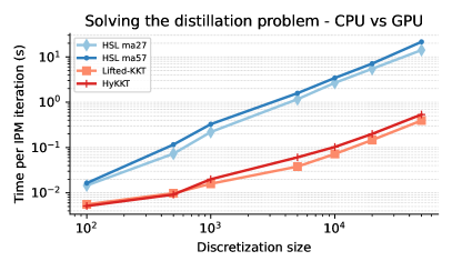
Figure 1: Time per IPM iterations (s), CPU versus GPU.

VII CONCLUSIONS AND FUTURE WORKS

VII-A Conclusions

In this paper, we have presented two hybrid solvers to solve the sparse KKT systems arising in IPM on the GPU: Lifted-KKT and HyKKT. We have implemented the two hybrid solvers within MadNLP, using the newly released cuDSS linear solver to compute the sparse Cholesky factorization on the GPU. Our results on the distillation column instance show that once the symbolic factorization is computed, both Lifted-KKT and HyKKT are significantly faster than HSL running on the CPU, with a time per iteration reduced by a factor of 25 on the largest instance.

VII-B Future Works

In this article, the dynamic structure of the problem (1) has not been exploited explicitly. However, it is known that for (1), the resulting condensed matrix $K_{k}$ is block-banded and can be factorized efficiently using a block-structured linear solver. Indeed, we can interpret $K_{k}$ as a matrix encoding a linear-quadratic program and solve the resulting problem in parallel using Dynamic Programming [7]. We are planning to investigate these promising outlooks in future research.

References

- [1] F. Allgöwer and A. Zheng, Nonlinear model predictive control, vol. 26. Birkhäuser, 2012.
- [2] S. J. Qin and T. A. Badgwell, “A survey of industrial model predictive control technology,” Control engineering practice, vol. 11, no. 7, pp. 733–764, 2003.
- [3] J. C. Dunn and D. P. Bertsekas, “Efficient dynamic programming implementations of Newton’s method for unconstrained optimal control problems,” Journal of Optimization Theory and Applications, vol. 63, no. 1, pp. 23–38, 1989.
- [4] V. M. Zavala, C. D. Laird, and L. T. Biegler, “Interior-point decomposition approaches for parallel solution of large-scale nonlinear parameter estimation problems,” Chemical Engineering Science, vol. 63, no. 19, pp. 4834–4845, 2008.
- [5] M. Diehl, H. J. Ferreau, and N. Haverbeke, “Efficient numerical methods for nonlinear MPC and moving horizon estimation,” Nonlinear model predictive control: towards new challenging applications, pp. 391–417, 2009.
- [6] C. Kirches, L. Wirsching, S. Sager, and H. G. Bock, “Efficient numerics for nonlinear model predictive control,” in Recent Advances in Optimization and its Applications in Engineering: The 14th Belgian-French-German Conference on Optimization, pp. 339–357, Springer, 2010.
- [7] S. J. Wright, “Partitioned dynamic programming for optimal control,” SIAM Journal on Optimization, vol. 1, no. 4, pp. 620–642, 1991.
- [8] C. V. Rao, S. J. Wright, and J. B. Rawlings, “Application of interior-point methods to model predictive control,” Journal of Optimization Theory and Applications, vol. 99, no. 3, pp. 723–757, 1998.
- [9] A. Cervantes and L. T. Biegler, “Large-scale DAE optimization using a simultaneous NLP formulation,” AIChE Journal, vol. 44, no. 5, pp. 1038–1050, 1998.
- [10] J. A. Andersson, J. Gillis, G. Horn, J. B. Rawlings, and M. Diehl, “CasADi: a software framework for nonlinear optimization and optimal control,” Mathematical Programming Computation, vol. 11, pp. 1–36, 2019.
- [11] H. J. Ferreau, C. Kirches, A. Potschka, H. G. Bock, and M. Diehl, “qpOASES: A parametric active-set algorithm for quadratic programming,” Mathematical Programming Computation, vol. 6, pp. 327–363, 2014.
- [12] J. V. Frasch, S. Sager, and M. Diehl, “A parallel quadratic programming method for dynamic optimization problems,” Mathematical programming computation, vol. 7, pp. 289–329, 2015.
- [13] G. Frison and M. Diehl, “HPIPM: a high-performance quadratic programming framework for model predictive control,” IFAC-PapersOnLine, vol. 53, no. 2, pp. 6563–6569, 2020.
- [14] R. Verschueren, G. Frison, D. Kouzoupis, J. Frey, N. v. Duijkeren, A. Zanelli, B. Novoselnik, T. Albin, R. Quirynen, and M. Diehl, “acados—a modular open-source framework for fast embedded optimal control,” Mathematical Programming Computation, vol. 14, no. 1, pp. 147–183, 2022.
- [15] G. Frison, D. Kouzoupis, T. Sartor, A. Zanelli, and M. Diehl, “BLASFEO: Basic linear algebra subroutines for embedded optimization,” ACM Transactions on Mathematical Software (TOMS), vol. 44, no. 4, pp. 1–30, 2018.
- [16] E. C. Kerrigan, G. A. Constantinides, A. Suardi, A. Picciau, and B. Khusainov, “Computer architectures to close the loop in real-time optimization,” in 2015 54th IEEE conference on decision and control (CDC), pp. 4597–4611, IEEE, 2015.
- [17] D.-K. Phung, B. Hérissé, J. Marzat, and S. Bertrand, “Model predictive control for autonomous navigation using embedded graphics processing unit,” IFAC-PapersOnLine, vol. 50, no. 1, pp. 11883–11888, 2017.
- [18] L. Yu, A. Goldsmith, and S. Di Cairano, “Efficient convex optimization on GPUs for embedded model predictive control,” in Proceedings of the General Purpose GPUs, (New York, NY, USA), pp. 12–21, Association for Computing Machinery, 2017.
- [19] K. M. M. Rathai, M. Alamir, and O. Sename, “GPU based stochastic parameterized NMPC scheme for control of semi-active suspension system for half car vehicle,” IFAC-PapersOnLine, vol. 53, no. 2, pp. 14369–14374, 2020.
- [20] S. Shin, F. Pacaud, and M. Anitescu, “Accelerating optimal power flow with GPUs: SIMD abstraction of nonlinear programs and condensed-space interior-point methods,” arXiv preprint arXiv:2307.16830, 2023.
- [21] A. Wächter and L. T. Biegler, “On the implementation of an interior-point filter line-search algorithm for large-scale nonlinear programming,” Mathematical Programming, vol. 106, no. 1, pp. 25–57, 2006.
- [22] M. Benzi, G. H. Golub, and J. Liesen, “Numerical solution of saddle point problems,” Acta numerica, vol. 14, pp. 1–137, 2005.
- [23] I. S. Duff and J. K. Reid, “The multifrontal solution of indefinite sparse symmetric linear,” ACM Transactions on Mathematical Software (TOMS), vol. 9, no. 3, pp. 302–325, 1983.
- [24] B. Tasseff, C. Coffrin, A. Wächter, and C. Laird, “Exploring benefits of linear solver parallelism on modern nonlinear optimization applications,” arXiv preprint arXiv:1909.08104, 2019.
- [25] K. Świrydowicz, E. Darve, W. Jones, J. Maack, S. Regev, M. A. Saunders, S. J. Thomas, and S. Peleš, “Linear solvers for power grid optimization problems: a review of GPU-accelerated linear solvers,” Parallel Computing, p. 102870, 2021.
- [26] D. Cole, S. Shin, F. Pacaud, V. M. Zavala, and M. Anitescu, “Exploiting GPU/SIMD architectures for solving linear-quadratic MPC problems,” in 2023 American Control Conference (ACC), pp. 3995–4000, IEEE, 2023.
- [27] F. Pacaud, S. Shin, M. Schanen, D. A. Maldonado, and M. Anitescu, “Accelerating condensed interior-point methods on SIMD/GPU architectures,” Journal of Optimization Theory and Applications, pp. 1–20, 2023.
- [28] S. Regev, N.-Y. Chiang, E. Darve, C. G. Petra, M. A. Saunders, K. Świrydowicz, and S. Peleš, “HyKKT: a hybrid direct-iterative method for solving KKT linear systems,” Optimization Methods and Software, vol. 38, no. 2, pp. 332–355, 2023.
- [29] G. H. Golub and C. Greif, “On solving block-structured indefinite linear systems,” SIAM Journal on Scientific Computing, vol. 24, no. 6, pp. 2076–2092, 2003.
- [30] J. Nocedal and S. J. Wright, Numerical optimization. Springer series in operations research, New York: Springer, 2nd ed., 2006.
- [31] N.-Y. Chiang and V. M. Zavala, “An inertia-free filter line-search algorithm for large-scale nonlinear programming,” Computational Optimization and Applications, vol. 64, pp. 327–354, 2016.
- [32] R. Verschueren, M. Zanon, R. Quirynen, and M. Diehl, “A sparsity preserving convexification procedure for indefinite quadratic programs arising in direct optimal control,” SIAM Journal on Optimization, vol. 27, no. 3, pp. 2085–2109, 2017.
- [33] W. Wan and L. T. Biegler, “Structured regularization for barrier NLP solvers,” Computational Optimization and Applications, vol. 66, pp. 401–424, 2017.
- [34] D. Thierry and L. Biegler, “The 1—exact penalty-barrier phase for degenerate nonlinear programming problems in Ipopt,” IFAC-PapersOnLine, vol. 53, no. 2, pp. 6496–6501, 2020.
- [35] G. Debreu, “Definite and semidefinite quadratic forms,” Econometrica: Journal of the Econometric Society, pp. 295–300, 1952.
- [36] M. H. Wright, “Ill-conditioning and computational error in interior methods for nonlinear programming,” SIAM Journal on Optimization, vol. 9, no. 1, pp. 84–111, 1998.
- [37] A. Montoison and D. Orban, “Krylov. jl: A julia basket of hand-picked krylov methods,” Journal of Open Source Software, vol. 8, no. 89, p. 5187, 2023.