Difference-in-Differences with Unpoolable Data

Abstract

In this study, we identify and relax the assumption of data “poolability” in difference-in-differences (DID) estimation. Poolability, or the combination of observations from treated and control units into one dataset, is often not possible due to data privacy concerns. For instance, administrative health data stored in secure facilities is often not combinable across jurisdictions. We propose an innovative approach to estimate DID with unpoolable data: UN–DID. Our method incorporates adjustments for additional covariates, multiple groups, and staggered adoption. Without covariates, UN–DID and conventional DID give identical estimates of the average treatment effect on the treated (ATT). With covariates, we show mathematically and through simulations that UN–DID and conventional DID provide different, but equally informative, estimates of the ATT. An empirical example further underscores the utility of our methodology. The UN–DID method paves the way for more comprehensive analyses of policy impacts, even under data poolability constraints.

Keywords: difference-in-differences, treatment effects, siloed data, unpooled data, impact evaluation

JEL Codes: C10, C12, C21, D04, I18, I38, Z18

1 Introduction

As economists, we are interested in evaluating the impact of a policy, both in attaining its intended objectives and in its unintended consequences. If the implementation or enforcement of a policy is randomized, we can easily estimate the average treatment effect on the treated (ATT) by comparing the means of the group that receives treatment and the group that does not. Under the more common non-randomized assignment to treatment, however, calculating the ATT is not straightforward due to selection bias. When policy changes are plausibly quasi-randomly assigned, difference-in-differences (DID) can be used to reasonably eliminate the selection bias and estimate the ATT.

The set of identifying assumptions for estimating the ATT in the DID framework includes parallel trends, no anticipation, no staggered adoption, and homogeneous treatment effect (Abadie, 2005; De Chaisemartin and d’Haultfoeuille, 2020a; Callaway and Sant’Anna, 2021). In the past five years, developments in the DID literature have explored what happens when each assumption is violated and how to identify the ATT under each violation. The source of identifying variation in DID analyses is often a policy change that occurs in some political jurisdictions (e.g., states, countries) but not in others. Treated observations come from jurisdictions or units in which the policy change occurs, while control or untreated observations come from jurisdictions that do not experience that change (at least not at the same time).

The strong correlation between treatment assignment and jurisdiction implies another important assumption that has not been addressed in the DID literature: the data from the treatment group and the control group can be combined together for analyses. If the identifying variation is supplied by policy variation across countries and the data come from an international survey, for example, this assumption can be met. Observations from both treated and control countries are already pooled together in the same dataset. However, in settings where the data come from the same jurisdictional level as the policy variation, country-level administrative data, for example, data from treated countries may not be poolable with data from control countries. In this case, the DID assumption of poolable data is not met, and DID cannot be used to estimate the ATT of a policy that varies at the country level.

In recent years, the types and sources of available data have expanded and now include detailed genetic, income, and mobility data, among others. In some cases, privacy concerns and data regulations result in such data being “siloed,” that is, combining data across jurisdictions or with other data sources even within jurisdictions is restricted or prohibited (Li et al., 2022). The disaggregated data needed to estimate the ATT with the conventional DID regression cannot be shared between treated and untreated jurisdictions and combined together on a single server. Therefore, using current DID approaches to estimate the ATT for policies that vary by jurisdiction and where the data are siloed at that same jurisdictional level is difficult, if not infeasible.

One example of within-country siloed data is in Canada, where the universal health-care system is decentralized among 13 provinces and territories, each overseeing health-care policy and delivery. Each jurisdiction has a “single payer” health insurance plan, which generates population-based claims data that contain individual characteristics and health-care services funded by the public insurer. Combining the changing and varied health policies and structures across Canadian jurisdictions with the DID methodology provides an excellent opportunity to understand their impacts in order to improve health-care system performance and population health. However, data poolability constraints have limited most such analyses to using within-province controls, to comparing first differences in treated and control provinces or to using surveys or other pooled data sources.

Similar data poolability challenges are encountered beyond health care and internationally across countries. For example, certain country-level datasets, like Canada’s Vital Statistics Mortality database and the United States’ administrative tax records, are housed in secure facilities, thereby siloing them and hindering their poolability with similar datasets from other countries. The issue of federated data extends beyond health economics to various research domains, including medical research, epidemiology, environmental science, social science, data science, and policy analysis. In cases where a policy, like the legalization of marijuana in Canada, impacts a whole country, employing a different country as a control group may be ideal to evaluate the policy’s impacts. Under data poolability constraints, the full benefits of DID estimation cannot be realized. Researchers often estimate treatment effects using within-jurisdiction variation, which may be more prone to selection bias, or by employing interrupted time series analysis (Bernal et al., 2017), which can generate biased estimates if other changes coincide with the intervention of interest.

Several journal articles in data science, medical engineering, and computer science have explored how siloed data can pose a barrier to research (Li et al., 2022; Hallock et al., 2021; Wang and Alexander, 2020). The heterogeneity of data distributions between silos, implying that the data may not be independently or identically distributed, makes analysis with siloed data difficult (Li et al., 2022). Siloed data likely reduces the adoption of hospital information systems, which further restricts data diffusion (McCullough, 2008). The literature has addressed a need for access to and poolability of health datasets (Hallock et al., 2021; Miller and Tucker, 2014; Wang and Alexander, 2020; McCullough, 2008). However, no papers have explored how to use siloed data to conduct DID analysis.

In this paper, we introduce a DID estimator that estimates the ATT with unpoolable data (UN) from the treated and control groups, which we call UN–DID. Because researchers commonly rely on regression-based tools for estimating treatment effects, the primary goal of this paper is to introduce the UN–DID estimator as a regression-based tool for this purpose. Through analytical proofs and a simulation study, we demonstrate that UN–DID can estimate relevant ATTs and their associated standard errors. The estimated ATTs from the UN–DID estimator are unbiased across various data-generating processes and converge to a common value with large sample sizes. This holds when we include both time-invariant and time-varying covariates. We also showcase a practical application of our methodology using two empirical examples.

2 Theoretical Framework

Let us assume that we have data for two groups, the treatment group and the control group, and data for several calendar years, $t=1,2,.....,T$. We also assume that the treatment was implemented at year $k$. Groups that received the treatment are called the treated group and groups that did not receive the treatment are called the control group. All calendar years before $k$ ($t<k$) are pooled together as the pre-intervention period. Similarly, all calendar years from $k$ onward ($t\geq k$) are pooled together as the post-intervention period. It is common practice to estimate DID using micro-level data of this nature, where numerous observations from individual subjects are available within each of the relevant cells.

The basic idea of DID estimation is to compare the difference in outcomes before and after the treatment between groups that received the treatment and groups that did not (Bertrand et al., 2004). The difference in outcomes between the treatment group and the control group before treatment is used to impute the unobserved counterfactual of the treated group. Card and Krueger (1993) first used the conventional DID to estimate the effect of an increase in minimum wage on unemployment in the American state of Pennsylvania. The traditional way of estimating the ATT involves running the following conventional regression:

$$Y^{S}_{i,t}=\beta_{0}+\beta_{1}D^{S}_{i}+\beta_{2}P^{S}_{t}+\beta_{3}P^{S}_{t}*D^{S}_{i}+\epsilon^{S}_{i,t}.$$ (1)

Here, $D^{S}_{i}$ is a dummy variable that takes on a value of 1 if individual $i$ is in the treatment group, and 0 otherwise. $P^{S}_{t}$ is a dummy variable that takes on a value of 1 if the data is for post-intervention period, and 0 otherwise. $S$ implies that we are combining the dataset from both the treated group $T$ and the control group $C$ into a common dataset ($S=T+C$). Under very strong assumptions, $\hat{\beta_{3}}$ (the coefficient of the interaction term between $D^{S}_{i}$ and $P^{S}_{t}$) identifies the ATT (Roth et al., 2022). To simplify notations, we will not use the $S$ superscripts to denote a combined dataset for the rest of the paper.

Assumption 1: Treatment is Binary

This implies individual $i$ can be either treated or not treated at time $t$. There are no variations in treatment intensity.

$$D_{i}=\begin{cases}1&\mbox{if individual i is treated at time t}.\\ 0&\mbox{if individual i is not treated at time t}.\\ \end{cases}$$

Assumption 2: Strong Parallel Tends

$$\begin{split}&\biggr{[}E[Y_{i}(0)|D_{i}=1,t=1]-E[Y_{i}(0)|D_{i}=1,t=0]\biggr{]}\\ &=\ \biggr{[}E[Y_{i}(0)|D_{i}=0,t=1]-E[Y_{i}(0)|D_{i}=0,t=0]\biggr{]}.\end{split}$$ (2)

Here, the $Y_{i}(0)$ are the untreated potential outcomes for the relevant group and period. Strong parallel trends imply that the evolution of outcome between treated and control groups immediately before treatment are the same. This ensures that the selection bias is 0 (Roth et al., 2022). When strong parallel trends hold, the ATT is shown in Equation (3). Refer to Callaway and Sant’Anna (2021) for a simple proof.

$$\footnotesize\begin{gathered}ATT=\biggl{[}E[Y_{i}|D_{i}=1,P_{t}=1]-E[Y_{i}|D_{i}=1,P_{t}=0]\biggr{]}-\biggl{[}E[Y_{i}|D_{i}=0,P_{t}=1]-E[Y_{i}|D_{i}=0,P_{t}=0]\biggr{]}.\end{gathered}$$ (3)

Here, $E[Y_{i}|D_{i}=1,P_{t}=1]$ is the expected outcome of the treated group in the post-intervention period and $E[Y_{i}|D_{i}=1,P_{t}=0]$ is the expected outcome of the treated group in the pre-intervention period. Similarly, $E[Y_{i}|D_{i}=0,P_{t}=1]$ is the expected outcome of the control group in the post-intervention period and $E[Y_{i}|D_{i}=0,P_{t}=0]$ is the expected outcome of the control group in the pre-intervention period.

Assumption 3: No Anticipation

No anticipation implies that treated units do not change behavior before treatment occurs (Abadie, 2005; De Chaisemartin and d’Haultfoeuille, 2020a). So, the treated potential outcome is equal to the untreated potential outcome for all units in the treated group in the pre-intervention period. Violation of no anticipation can also lead to deviations in parallel trends before treatment. Here, $Y_{i}(t)$ is the treated potential outcome of individual $i$ at calendar year $t$.

$$\begin{gathered}\biggl{[}E[Y_{i}(t)|D_{i}=1,P_{t}=0]=E[Y_{i}(0)|D_{i}=1,P_{t}=0]\biggr{]}\mbox{\quad{a.s.} for all}\;\;t<k.\end{gathered}$$ (4)

Assumption 4: Homogeneous Treatment Effect Homogeneous treatment effect implies that all treated units have the same treatment effect across both time and individuals. Formally, it means that the difference in potential outcomes for treated units is the same for all time periods after treatment.

$$\begin{gathered}\biggl{[}E[Y_{i}(t)|D_{i}=1,P_{t}=1]-E[Y_{i}(0)|D_{i}=1,P_{t}=1]\biggr{]}\\ =\biggl{[}E[Y_{j}(t)|D_{j}=1,P_{t}=1]-E[Y_{j}(0)|D_{j}=1,P_{t}=1]\biggr{]}\mbox{\quad{a.s.} for all}\;\;i\neq j.\end{gathered}$$ (5)

Assumption 5: No Staggered Adoption

No staggered adoption implies treatment occurs only once (Callaway and Sant’Anna, 2021; De Chaisemartin and d’Haultfoeuille, 2020a). Formally, it means that all units in the treated group are treated at calendar year $k$. Throughout this paper, we maintain the above assumptions unless stated otherwise.

In recent years, much work has been done in the DID literature to investigate what occurs when each of the aforementioned assumptions are violated. In this paper, we introduce a new assumption that has been implied in previous literature but has not been explicitly explored or discussed in the context of DID.

Assumption 6: Data is Poolable

Data from the treatment and control groups are available on a single server and can be combined together for analyses. Let $T$ and $C$ be two data silos, where $T$ is the treated silo and $C$ is the untreated silo. $Y_{T}$ and $Y_{C}$ are two matrices containing data for the outcome variable for silo $T$ and $C$, respectively, and $N_{T}$ and $N_{C}$ the total number of observations in the matrices, respectively.

$$Y_{T}=\begin{bmatrix}y_{T1}\\ y_{T2}\\ \vdots\\ y_{TN_{T}}\end{bmatrix},Y_{C}=\begin{bmatrix}y_{C1}\\ y_{C2}\\ \vdots\\ y_{CN_{C}}\end{bmatrix}$$

Under the poolability assumption, the two matrices can be stacked together into a common matrix Y, which is not feasible when there are legal restrictions preventing them from being stacked together (or data are unpooled):

$$Y=\begin{bmatrix}Y_{T}\\ Y_{C}\end{bmatrix}=\begin{bmatrix}y_{T1}\\ y_{T2}\\ \vdots\\ y_{TN_{T}}\\ y_{C1}\\ y_{C2}\\ \vdots\\ y_{CN_{C}}\end{bmatrix}$$

For situations where Assumption 6 is violated, we introduce the UN–DID approach, which can estimate the ATT in scenarios where the data is not poolable. With unpoolable data, when we access the data from the treated silo, we have no knowledge of the data from the control group, $Y_{C}$. Similarly, once we have access to the data from the untreated silo, we have no information about the data from the treated silo, or $Y_{T}$. We know only the treatment status of the individuals in each silo and whether the data are from the pre- or post-intervention period. The conventional method becomes impractical in situations when data are segregated, or is “siloed,” because datasets cannot be combined for conventional regression analysis.

In this case, we can visit each silo and run regressions shown in equations (6) and (7) for the treated and untreated silos, respectively. In the simplest case, we assume that there are only two silos: the treated silo ($T$) and the untreated silo ($C$). We also assume that there are no covariates. Here, $Y^{T}_{i,t}$ is the outcome for an individual from the silo that is treated at time $t$ and $Y^{C}_{i,t}$ is the outcome of an individual from the silo that is untreated at time $t$. $post_{t}^{T}$ is a dummy variable that takes on a value of 1 when the treated observation is in the post-intervention period, and 0 otherwise. Similarly, $post_{t}^{C}$ is a dummy variable that takes on a value of 1 when the untreated observation is in the post-intervention period, and 0 otherwise. $pre_{t}^{T}$ is a dummy variable that takes on a value of 1 if the treated observation is in the pre-intervention period, hence $pre_{t}^{T}=1-post_{t}^{T}$. Similarly, $pre_{t}^{C}$ is a dummy variable that takes on a value of 1 if the untreated observation is in the pre-intervention period, hence $pre_{t}^{C}=1-post_{t}^{C}$. Note that the regressions in equations (6) and (7) are done without a constant. Therefore, none of the variables are dropped because of multicollinearity.

$$\mbox{For treated:}\;Y^{T}_{i,t}=\lambda_{1}^{T}pre_{t}^{T}+\lambda_{2}^{T}post_{t}^{T}+\nu^{T}_{i,t}$$ (6)

$$\mbox{For untreated:}\;Y^{C}_{i,t}=\lambda_{1}^{C}pre_{t}^{C}+\lambda_{2}^{C}post_{t}^{C}+\nu^{C}_{i,t}$$ (7)

These regressions are silo-specific. Because data are siloed, the treated regression does not contain any data from the untreated silo and the untreated regression does not contain any data from the treated silo. Here, $(\widehat{\lambda_{2}^{T}}-\widehat{\lambda_{1}^{T}})-(\widehat{\lambda_{2}^{C}}-\widehat{\lambda_{1}^{C}})$ is the estimate of the ATT, as shown in Equation (8). The associated standard error of the ATT is estimated as the square root of the sum of the standard errors used to estimate the ATT estimated from the above UN–DID regressions. This is shown in Equation (9).

$$\widehat{ATT}=(\widehat{\lambda_{2}^{T}}-\widehat{\lambda_{1}^{T}})-(\widehat{\lambda_{2}^{C}}-\widehat{\lambda_{1}^{C}}).$$ (8)

$$\widehat{SE}(\widehat{ATT})=\sqrt{\widehat{SE}(\widehat{\lambda_{1}^{T}})^{2}+\widehat{SE}(\widehat{\lambda_{2}^{T}})^{2}+\widehat{SE}(\widehat{\lambda_{1}^{C}})^{2}+\widehat{SE}(\widehat{\lambda_{2}^{C}})^{2}}.$$ (9)

2.1 Cluster-Robust Inference

In this paper, we assume that the error terms are independent. Accordingly, we can estimate standard errors that are robust to heteroskedasticity but not robust to clustering. Cluster-robust inference is challenging when models like those in equations (6) and (7) are estimated at the silo level. Researchers typically will cluster at the level of the policy change, which is the silo in this case. Conventional methods of cluster-robust inference will not work with silo-specific data because there is only one cluster in each dataset. Work in progress by the authors of this paper aims to extended these methods to allow for cluster-robust inference.

3 UN–DID When Strong Parallel Trends Hold

In this section, we assume that the strong parallel trends assumption is plausible between the treated and untreated silos. We also assume that no anticipation, homogeneous treatment effects, and no staggered adoption hold. Under these assumptions, we show that the UN–DID and the conventional DID recover the same estimate of the ATT when strong parallel trends hold, both analytically and through a Monte Carlo simulation study.

3.1 Equivalence of the Estimated ATT Between Conventional and UN–DID Methods with No Covariates

Conventional Regression

Under assumptions 1 to 6, $\hat{\beta_{3}}$ in the regression shown in Equation (10) is the estimate of the ATT (Roth et al., 2022). Note that the conventional regression can be used only if the data poolability assumption holds. For simplicity of notation, we assign all calendar years in the pre-intervention period as $t=0$ and assign all calendar years in the post-intervention period as $t=1$.

$$Y_{i,t}=\beta_{0}+\beta_{1}D_{i}+\beta_{2}P_{t}+\beta_{3}P_{t}*D_{i}+\epsilon_{i,t}.$$ (10)

Now we will prove that $\hat{\beta_{3}}$ is the sample analogue of Equation (3), or the estimate of the ATT. According to the Frisch–Waugh–Lowell (FWL) theorem, $\hat{\beta_{3}}$ will be the same as the coefficient of $(P_{t}*D_{i}-\widehat{P_{t}*D_{i}})$ from the regression shown in Equation (12). Here, $(P_{t}*D_{i}-\widehat{P_{t}*D_{i}})$ are the residuals from the regression shown in Equation (11).

$$P_{t}*D_{i}=\alpha_{0}+\alpha_{1}P_{t}+\alpha_{2}D_{i}+u_{i,t}.$$ (11)

$$Y_{i,t}=\widehat{\beta_{3}}(P_{t}*D_{i}-\widehat{P_{t}*D_{i}})+u^{\prime}_{i,t}.$$ (12)

From Equation (12), we compute the residuals ($P_{t}*D_{i}-\widehat{P_{t}*D_{i}}$) for each observation. For a treated observation in the pre-intervention period, the residual is given by $-\hat{\alpha_{0}}-\hat{\alpha_{2}}$. Conversely, for a treated observation in the post-intervention period, the residual becomes $1-\hat{\alpha_{0}}-\hat{\alpha_{1}}-\hat{\alpha_{2}}$. Similarly, an untreated observation in the pre-intervention period has a residual of $-\hat{\alpha_{0}}$, while an untreated observation in the post-intervention period yields a residual of $-\hat{\alpha_{0}}-\hat{\alpha_{1}}$. The residuals for all individuals in their respective cohort are the same, as shown by De Chaisemartin and d’Haultfoeuille (2020a). We then proceed to derive $\widehat{\beta_{3}}$ from Equation (12) by using the following OLS formula:

$$\begin{split}\hat{\beta}_{3}=&\sum_{i}\sum_{t}\frac{Y_{i,t}\left(P_{t}*D_{i}-\widehat{P_{t}*D_{i}}\right)}{\left(P_{t}*D_{i}-\widehat{P_{t}*D_{i}}\right)^{2}}.\end{split}$$ (13)

We can substitute the computed residuals into the numerator and simplify the expression from Equation (13) as outlined below:

$$\begin{split}&\sum_{i\in t=0,T}Y_{i,0}^{T}\left(-\hat{\alpha}_{0}-\hat{\alpha}_{2}\right)+\sum_{i\in t=1,T}Y_{i,1}^{T}\left(1-\hat{\alpha}_{0}-\hat{\alpha}_{1}-\hat{\alpha}_{2}\right)+\\ &\sum_{i\in t=0,C}Y_{i,1}^{C}\left(1-\hat{\alpha}_{0}-\hat{\alpha}_{1}-\hat{\alpha}_{2}\right)+\sum_{i\in t=1,C}Y^{C}_{i,1}\left(-\hat{\alpha}_{0}-\hat{\alpha}_{1}\right).\end{split}$$

Likewise, by substituting the residuals and simplifying, the denominator of Equation (13) can be expressed as

$$\begin{split}A=\sum_{i\in t=0,T}\left(-\hat{\alpha}_{0}-\hat{\alpha}_{2}\right)^{2}+\sum_{i\in t=1,T}\left(1-\hat{\alpha}_{0}-\hat{\alpha}_{1}-\hat{\alpha}_{2}\right)^{2}+\sum_{i\in t=0,C}\left(-\hat{\alpha}_{0}\right)^{2}+\sum_{i\in t=1,C}\left(-\hat{\alpha}_{0}-\hat{\alpha}_{1}\right)^{2}.\end{split}$$

The denominator is the sum of squared residuals from the regression in Equation (11). Combining the numerator and the denominator, $\hat{\beta_{3}}$ can be written as

$$\begin{split}\hat{\beta}_{3}=&\frac{\left(1-\hat{\alpha}_{0}-\hat{\alpha}_{1}-\hat{\alpha}_{2}\right)\sum_{i\in t=1,T}Y_{i,1}^{T}}{A}-\frac{\left(\hat{\alpha}_{0}+\hat{\alpha}_{2}\right)\sum_{i\in t=0,T}Y_{i,0}^{T}}{A}\\ &-\frac{\left(\hat{\alpha}_{0}+\hat{\alpha}_{1}\right)\sum_{i\in t=1,C}Y_{i,1}^{C}}{A}+\frac{\left(-\hat{\alpha_{0}}\right)\sum_{i\in t=0,C}Y_{i,0}^{C}}{A}.\end{split}$$ (14)

In Appendix A, we show that $\frac{\left(1-\hat{\alpha}_{0}-\hat{\alpha}_{1}-\hat{\alpha}_{2}\right)}{A}$ is the reciprocal of the number of observations in the the treated group and the post-intervention period ($N_{1,1})$ and $\frac{\left(\hat{\alpha}_{0}+\hat{\alpha}_{2}\right)}{A}$ is the reciprocal of the number of observations in the treated group in the pre-intervention period ($N_{1,0}$). Similarly, $\frac{\left(\hat{\alpha}_{0}+\hat{\alpha}_{2}\right)}{A}$ is the reciprocal of the number of observations in the control group in the post-intervention period $(N_{0,1})$ and $\frac{\left(-\hat{\alpha}_{0}\right)}{A}$ is reciprocal of the number of observations in the control group in the pre-intervention period ($N_{0,0})$. Therefore, Equation (14) can be further simplified as

$$\begin{split}\hat{\beta}_{3}=\frac{1}{N_{1,1}}\sum_{i\in t=1,T}Y_{i,1}^{T}-\frac{1}{N_{1,0}}\sum_{i\in t=0,T}Y_{i,0}^{T}-\frac{1}{N_{0,1}}\sum_{i\in t=1,C}Y_{i,1}^{C}+\frac{1}{N_{0,0}}\sum_{i\in t=0,C}Y_{i,0}^{C}\end{split}$$

$$\begin{split}\Rightarrow\hat{\beta}_{3}=&\left(\overline{Y^{T}_{i,1}}-\overline{Y^{T}_{i,0}}\right)-\left(\overline{Y^{C}_{i,1}}-\overline{Y^{C}_{i,0}}\right).\end{split}$$ (15)

In simpler notation, Equation (15) can be rewritten as

$$\begin{split}\hat{\beta}_{3}=&\left(\overline{Y}_{D_{i}=1,P_{t}=1}-\overline{Y}_{D_{i}=1,P_{t}=0}\right)-\left(\overline{Y}_{D_{i}=0,P_{t}=1}-\overline{Y}_{D_{i}=0,P_{t}=0}\right).\end{split}$$ (16)

Equation (16) is the sample analogue of the ATT under strong parallel trends shown in Equation (3).

UN–DID Regression

In this subsection, we hold that Assumption 6 is violated (data are no longer poolable), while assumptions 1 to 5 hold. Under the violation of Assumption 6, the conventional regression can no longer be used to estimate the ATT. Under these assumptions, we prove that $(\widehat{\lambda_{2}^{T}}-\widehat{\lambda_{1}^{T}})-(\widehat{\lambda_{2}^{C}}-\widehat{\lambda_{1}^{C}})$ derived from the UN–DID regressions can recover the estimate of the ATT. Additionally, we demonstrate that the ATT obtained through the UN–DID regression is numerically equal to the conventional ATT estimate given that the samples used for both approaches are the same. Equations (6) and (7) can be rewritten in the following way:

$$\;Y^{j}_{i,t}=\lambda_{1}^{j}pre_{t}^{j}+\lambda_{2}^{j}post_{t}^{j}+\nu^{j}_{i,t},\;\;\;\;\;\;\mbox{where}\;j=\{T,C\}.$$ (17)

$$\equiv\;Y^{j}_{i,t}=\gamma_{0}^{j}+\gamma_{1}^{j}post_{t}^{j}+\nu^{j}_{i,t},\;\;\;\;\;\;\mbox{where}\;j=\{T,C\}.$$ (18)

It can be shown that Equation (17) is equivalent to Equation (18).

Proof: We know that $pre_{t}^{j}=(1-post_{t}^{j})$. Substituting this into Equation (17) gives

$$Y^{j}_{i,t}=\lambda_{1}^{j}(1-post_{t}^{j})+\lambda_{2}^{j}post_{t}^{j}+\nu^{j}_{i,t}$$

$$\Rightarrow{Y^{j}_{i,t}}=\lambda_{1}^{j}+(\lambda_{2}^{j}-\lambda_{1}^{j})\text{post}_{t}^{j}+\nu^{j}_{i,t}.$$ (19)

Comparing equations (18) and (19), we can see that $\lambda_{1}^{j}=\gamma_{0}^{j}$ and $(\lambda_{2}^{j}-\lambda_{1}^{j})=\lambda_{2}^{j}$. Now we will prove that $(\widehat{\lambda_{2}^{T}}-\widehat{\lambda_{1}^{T}})-(\widehat{\lambda_{2}^{C}}-\widehat{\lambda_{1}^{C}})=\hat{\gamma_{1}^{T}}-\hat{\gamma_{1}^{C}}$ is the sample analogue of the ATT shown in Equation (3). In Equation (18), the coefficient of interest is $\hat{\gamma^{j}_{1}}$. According to the FWL theorem, $\hat{\gamma^{j}_{1}}$ will be the same as the coefficient of $(post_{t}^{j}-\widehat{post_{t}^{j}})$ from the regression shown in Equation (21). Here, $(post_{t}^{j}-\widehat{post_{t}^{j}})$ are the residuals from the regression shown in Equation (20).

$$post_{t}^{j}=\eta_{0}^{j}+\omega^{j}_{i,t},\;\;\;\;\;\;\mbox{where}\;\;\;\eta_{0}^{j}=\overline{post_{t}^{j}}.$$ (20)

$$Y_{i,t}^{j}=\widehat{\gamma_{1}^{j}}(post^{j}_{t}-\widehat{post^{j}_{t}})+\nu^{j^{\prime}}_{i,t}.$$ (21)

Similar to in the preceding subsection, we calculate the residuals $(post_{t}^{j}-\widehat{post_{t}^{j}})$ for each observation using Equation (20). For an observation in group j during the pre-intervention period, the residual is given by $(post^{j}_{t}-\widehat{post^{j}_{t}})=-\hat{\eta_{0}^{j}}$. Likewise, for an observation in group j during the post-intervention period, the residual becomes $(post^{j}_{t}-\widehat{post^{j}_{t}})=1-\hat{\eta_{0}^{j}}$. Following this, we proceed to obtain $\widehat{\gamma_{1}^{j}}$ from Equation (21) using the OLS formula:

$$\begin{split}\hat{\gamma}_{1}^{i}=&\frac{\sum_{i}\sum_{t}Y_{i,t}^{j}\left(post^{j}_{t}-\hat{post}^{j}_{t}\right)}{\sum_{i}\sum_{t}\left(post^{j}_{t}-\hat{post}^{j}_{t}\right)^{2}}\\ \Rightarrow\hat{\gamma}_{1}^{j}=&\frac{\sum_{i\in t=0}Y_{i,t}^{j}\left(-\hat{\eta}_{0}^{j}\right)+\sum_{i\in t=1}Y_{i,t}^{j}\left(1-\hat{\eta}_{0}^{j}\right)}{\sum_{i\in t=0}\left(-\hat{\eta}_{0}^{j}\right)^{2}+\sum_{i\in t=1}\left(1-\hat{\eta}_{0}^{j}\right)^{2}}\\ \Rightarrow\hat{\gamma}_{1}^{j}=&\frac{1-\hat{\eta}_{0}^{j}}{\sum_{i\in t=0}\left(-\hat{\eta}_{0}^{j}\right)^{2}+\sum_{i\in t=1}\left(1-\hat{\eta}_{0}^{j}\right)^{2}}\sum_{i\in t=1}Y_{i,1}\\ &-\frac{\hat{\eta}_{0}^{j}}{\sum_{i\in t=0}\left(-\hat{\eta}_{0}^{j}\right)^{2}+\sum_{i\in t=1}\left(1-\hat{\eta}_{0}^{j}\right)^{2}}\sum_{i\in t=0}Y_{i,0},\end{split}$$

$$\hat{\gamma}_{1}^{j}=\frac{1-\hat{\eta}_{0}^{j}}{B}\sum_{i\in t=1}Y_{i,1}-\frac{\hat{\eta}_{0}^{j}}{B}\sum_{i\in t=0}Y_{i,0}.\quad$$ (22)

Here, $B=\sum_{i\in t=0}\left(-\hat{\eta}_{0}^{j}\right)^{2}+\sum_{i\in t=1}\left(1-\hat{\eta}_{0}^{j}\right)^{2}$. Following the proof in Appendix A, $\frac{1-\hat{\eta}_{0}^{j}}{B}$ is the reciprocal of the number of observations in group $j$ in the post-intervention period and $\frac{\hat{\eta}_{0}^{j}}{B}$ is the reciprocal of the number of observations in group j for the pre-intervention period. Therefore, Equation (22) can be rewritten as

$$\hat{\gamma}_{1}^{j}=\frac{1}{N_{j,1}}\sum_{i\in t=1}Y_{i,1}-\frac{1}{N_{j,0}}\sum_{i\in t=0}Y_{i,0}$$

$$\Rightarrow\hat{\gamma}_{1}^{j}=\left(\overline{Y^{j}_{i,1}}-\overline{Y^{j}_{i,0}}\right).$$ (23)

From Equation (23), we can take the difference between $\hat{\gamma^{T}_{1}}$ and $\hat{\gamma^{C}_{1}}$ from the treated and untreated regressions, respectively. Equation (24) shows that the difference is the sample analogue of the ATT shown in Equation (3). If we compare equations (16) and (25), we can see that the conventional estimates and the UN–DID estimates provide numerically equal estimates of the ATT. Note that the conventional regression is not possible with data that are siloed. This is a hypothetical scenario where we assume that we can combine data from different silos together and run both the conventional and the UN–DID regressions on the data. In this case, both methods can identify the ATT and give equivalent estimates:

$$\begin{split}\hat{\gamma}_{1}^{T}-\hat{\gamma}_{1}^{C}=\left(\overline{Y^{T}_{i,1}}-\overline{Y^{T}_{i,0}}\right)-\left(\overline{Y^{C}_{i,1}}-\overline{Y^{C}_{i,0}}\right)\end{split}$$

$$\begin{split}\Rightarrow(\widehat{\lambda_{2}^{T}}-\widehat{\lambda_{1}^{T}})-(\widehat{\lambda_{2}^{C}}-\widehat{\lambda_{1}^{C}})=\left(\overline{Y^{T}_{i,1}}-\overline{Y^{T}_{i,0}}\right)-\left(\overline{Y^{C}_{i,1}}-\overline{Y^{C}_{i,0}}\right).\end{split}$$ (24)

In simpler notation, Equation (24) can be rewritten as

$$\begin{split}(\widehat{\lambda_{2}^{T}}-\widehat{\lambda_{1}^{T}})-(\widehat{\lambda_{2}^{C}}-\widehat{\lambda_{1}^{C}})=&\left(\overline{Y}_{D_{i}=1,P_{t}=1}-\overline{Y}_{D_{i}=1,P_{t}=0}\right)-\left(\overline{Y}_{D_{i}=0,P_{t}=1}-\overline{Y}_{D_{i}=0,P_{t}=0}.\right)\end{split}$$ (25)

3.2 Monte Carlo Design

We conduct a set of Monte Carlo experiments with synthetic data to demonstrate the unbiasedness of the UN–DID estimator and its relative performance compared with the conventional estimator. The overall experiment is depicted in Figure 1, where we apply both conventional and UN–DID regression methods to the same simulated dataset to estimate ATT and assess their properties. Note that, with poolable data, we can apply both the conventional and UN–DID methods to estimate the ATT. With unpoolable data, we are not able to run the conventional regression. Because these are synthetic data, they are poolable. Therefore, we can run both methods on the datasets simultaneously.

Our generated dataset is intended to replicate samples from census data for Ontario and Quebec, specifically concentrating on individuals aged 65 and above. To be more precise, we aligned the age and gender distributions to closely resemble those observed in the populations of Quebec and Ontario in 2001 for individuals aged 65 years and older. We keep the gender constant for all individuals and age them by one year for the next eight years, resulting in our final dataset. In our initial simulation, we created groups of 50 individuals each in both Ontario and Quebec, covering the period from 2000 to 2009. This results in a total of 500 observations evenly distributed over 10 years. We chose a small sample size to ensure the robustness of the results even when dealing with small datasets. For the simulation, we assume that Quebec is treated by some arbitrary policy in the year 2005. This approach ensures a balanced and symmetrical dataset, maintaining an equal number of observations in both pre- and post-treatment periods and in the treatment and control groups. We then repeat the simulations with roughly two thirds of the total observations in Ontario and one third of the total observations in Quebec. So, in a DGP with 500 observations, roughly 333 of the observations are in Ontario and 167 are in Quebec.

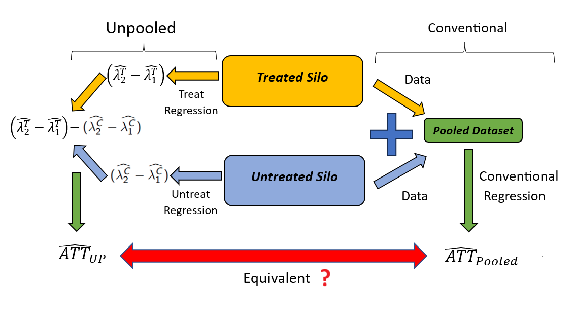
Figure 1: Schematic for Simulations

We also consider two data-generating processes to assess whether the estimates of the ATT align between conventional and UN–DID regressions. In the first case, we set the true treatment effect for the treated group at 0. In the second case, the true treatment effect for the treated group is set at 0.1. After generating the data, we perform both conventional and UN–DID regressions to estimate the ATT and access their unbiasedness properties. This is then repeated 1,000 times for each case. The data-generating process for the two cases are as follows:

• Case 1: No treatment effect, no covariates:

  $$Y^{g}_{it}=e^{g}_{it}.$$

• Case 2: Treatment effect, no covariates:

  $$Y^{g}_{it}=0.1*DID^{g}_{it}+e^{g}_{it}.$$

In all the simulations in the paper, the error term is idiosyncratic and follows a normal distribution, denoted as $e\sim\mathcal{N}(0,1)$. The $DID^{g}_{it}$ represents the interaction term between $P_{t}$ and $D_{i}$, corresponding to the post and treat dummy variables. The coefficient associated with this interaction term signifies the “true” effect of the treatment in both cases.

3.3 Results: No Covariates

In subsection 3.1, we have shown that the estimated ATT between the conventional and the UN–DID regressions are exactly numerically equivalent. To gain a more intuitive understanding of why the estimates from conventional and UN–DID regressions are equal, it is helpful to delve into the interpretation of the coefficients in the UN–DID regressions. Specifically, $\widehat{\lambda_{2}^{T}}$ represents the mean outcome of the treated group in the post-intervention period, while $\widehat{\lambda_{1}^{T}}$ signifies the mean outcome of the treated group in the pre-intervention period. Similarly, $\widehat{\lambda_{2}^{C}}$ corresponds to the mean outcome of the control group in the post-intervention period and $\widehat{\lambda_{1}^{C}}$ denotes the mean outcome of the control group in the pre-intervention period.

Proof: Rewriting Equation (6) and taking expectation conditional on $pre_{t}^{T}=1$ on both sides, we get

$$Y^{T}_{i,t}=\lambda_{1}^{T}pre_{t}^{T}+\lambda_{2}^{T}post_{t}^{T}+\nu^{T}_{i,t}$$

$$\Rightarrow E[Y^{T}_{i,t}|pre_{t}^{T}=1]=E[\lambda_{1}^{T}pre_{t}^{T}|pre_{t}^{T}=1]+E[\lambda_{2}^{T}post_{t}^{T}|pre_{t}^{T}=1]+E[\nu^{T}_{i,t}pre_{t}^{T}=1]$$

$$\Rightarrow E[Y^{T}_{i,t}|pre_{t}^{T}=1]=\lambda_{1}^{T}E[pre_{t}^{T}|pre_{t}^{T}=1]+\lambda_{2}^{T}E[post_{t}^{T}|pre_{t}^{T}=1].$$

Here, $E[\nu^{T}_{i,t}]=0$ by the strong exogeneity condition due to i.i.d sampling assumption. Because $pre_{t}^{T}=1$ is a dummy variable, we know that $E[pre_{t}^{T}|pre_{t}^{T}=1]=1$. By definition, we also know that $E[post_{t}^{T}|pre_{t}^{T}=1]=0$ because $post_{t}^{T}=1-pre_{t}^{T}$. Plugging in these values, we can rewrite the above equation as

$$E[Y^{T}_{i,t}|pre_{t}^{T}=1]=\lambda_{1}^{T}.$$

Therefore, the estimate of $\lambda_{1}^{T}$ is the mean outcome of the treated group in the pre-intervention period. Taking the expectation conditional on $post_{t}^{T}=1$ on both sides, we can also show that $E[Y^{T}_{i,t}|post_{t}^{T}=1]=\lambda_{2}^{T}$. The same can be shown for $\lambda_{1}^{C}$ and $\lambda_{2}^{T}$.

A more formal proof of the interpretations is shown in subsection 3.1. Therefore, $(\widehat{\lambda_{2}^{T}}-\widehat{\lambda_{1}^{T}})-(\widehat{\lambda_{2}^{C}}-\widehat{\lambda_{1}^{C}})$ is an estimate of the ATT shown in Equation (3). In subsection 3.1, we also establish that $\widehat{\beta_{3}}=\left(\overline{Y}_{D_{i}=1,P_{t}=1}-\overline{Y}_{D_{i}=1,P_{t}=0}\right)-\left(\overline{Y}_{D_{i}=0,P_{t}=1}-\overline{Y}_{D_{i}=0,P_{t}=0}\right)$. Here, $\overline{Y}_{D_{i}=k,P_{t}=l}$ represents the mean outcome of group $k$ in period $l$. When the law of large numbers holds, $\widehat{\beta_{3}}$ serves as the estimate of the ATT, as indicated in Equation (3). Assuming the sample is identical for both the conventional and UN–DID methods, both estimators should yield equal estimates of the ATT and their associated standard errors.

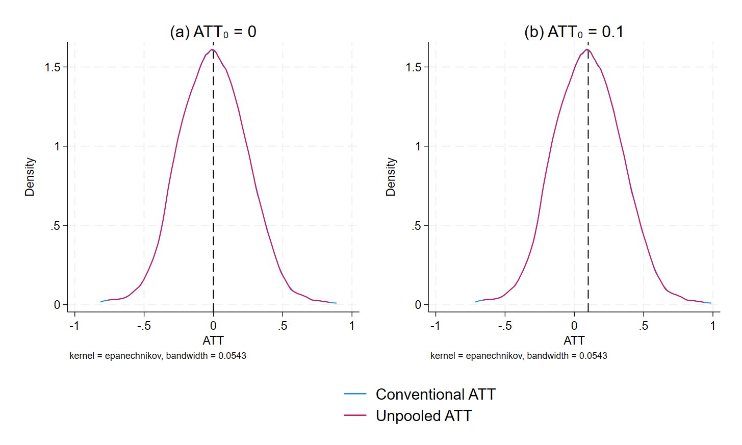
Figure 2: No Covariates with Unequal Sample Sizes: Kernel Density

The simulation study with equal sample sizes demonstrates that the UN–DID estimator is unbiased. To assess unbiasedness, we proceed to generate kernel density plots for both conventional and UN–DID estimates of the ATT on a shared axis. The kernel densities for unequal sample sizes are shown in Figure 2. In Panel (a), the kernel density estimates for Case 1 are presented, and in Panel (b), the kernel density estimates for Case 2 are presented. Notably, for Case 1, both kernels are centered around 0, aligning with the true value of the ATT. Similarly, for Case 2, both kernels are centered around 0.1, which is the true value of the ATT for Case 2. This finding demonstrates that both conventional and UN–DID estimation methods exhibit unbiasedness, as evidenced by the distributions of estimates being centered around the true values of the ATT. A similar pattern is found with equal sample sizes, in a figure not included.

In order to prove whether the UN–DID approaches the true value as sample size increases, we repeat the Monte Carlo simulation by increasing the sample size to 1,000, 2,000, 4,000, 8,000, 10,000, and 50,000 while maintaining equal sample sizes between both silos. Subsequently, we compute the mean squared error (MSE) between the estimated ATT using UN–DID and the true ATT from the underlying DGP according to Equation (26):

$$MSE(\widehat{ATT})=\frac{1}{1000}\sum_{j}^{1000}\biggl{(}\widehat{ATT_{j}}^{Unpooled}-ATT_{0}\biggr{)}^{2}.$$ (26)

To determine the MSE of the standard errors, we initially calculate the true standard error of the ATT using the following formula:

$$SE_{0}=\frac{\sum_{i}e^{2}}{(n-f)(DID-\overline{DID})^{2}}.$$ (27)

Here, $\overline{DID}$ is the mean of the DID term from the generated dataset and $f$ is the degrees of freedom. In the case with no covariates, the degrees of freedom is set at 4, following the conventional regression shown in Equation (1). The MSEs for the standard errors are then computed using the formula shown in Equation (28):

$$MSE(\widehat{SE})=\frac{1}{1000}\sum_{j}^{1000}\biggl{(}\widehat{SE}(\widehat{ATT_{j}})^{Unpooled}-SE_{0}\biggr{)}^{2}.$$ (28)

The findings are shown in Figure 3, where the y-axis represents the mean squared error (MSE) and the x-axis corresponds to the sample size. The graph illustrates a decreasing trend in MSE for both the estimated ATT and the standard error as the sample size increases. The results for unequal sample sizes are illustrated in Figure 4. We observe that the MSE for the case with unequal sample sizes is higher than for the case with equal sample sizes but still converges to 0 as sample size increases.

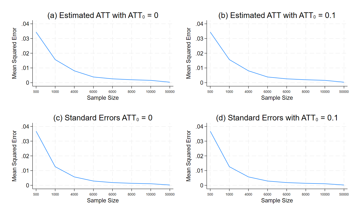
Figure 3: No Covariates with Equal Sample Sizes: Mean Squared Errors

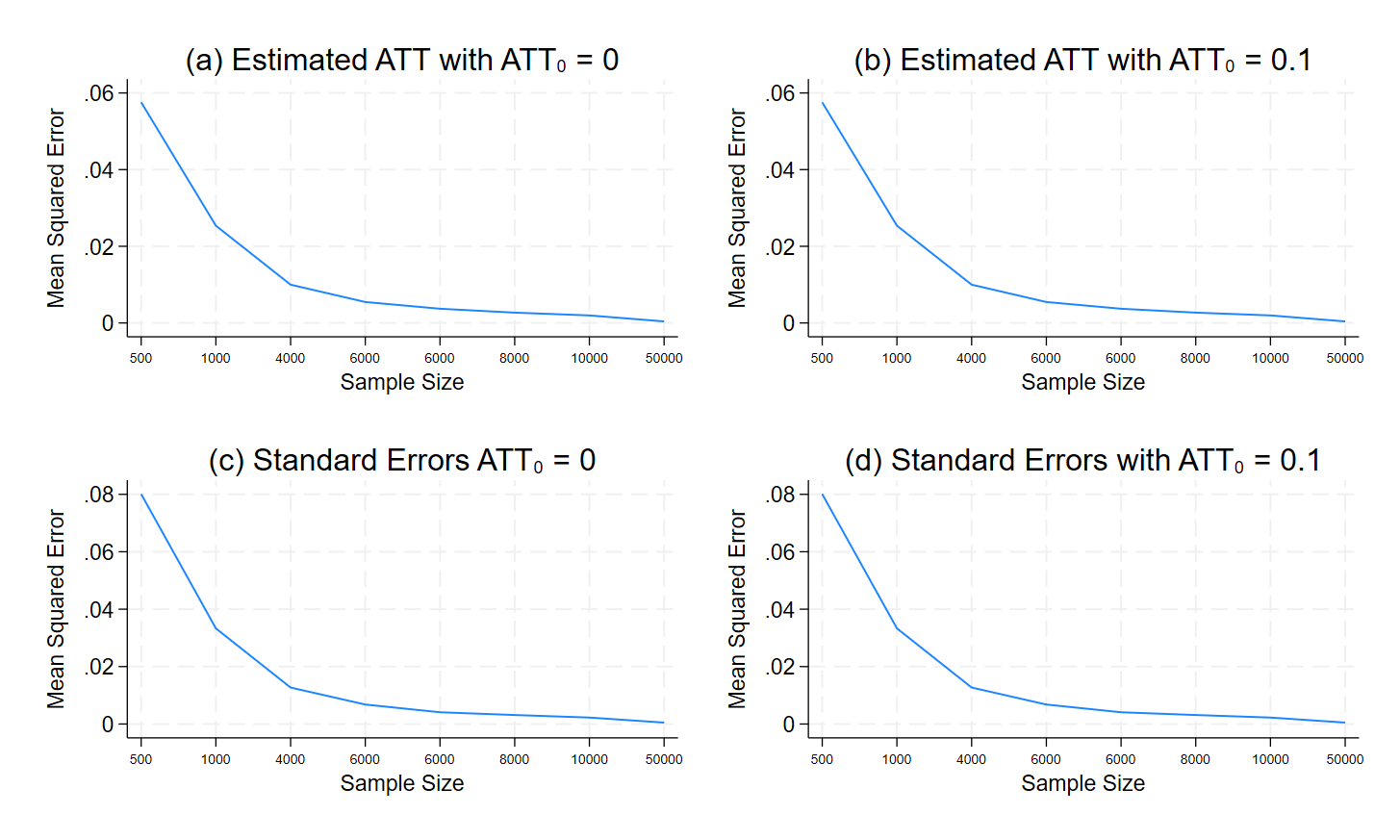
Figure 4: No Covariates with Equal Sample Sizes: Mean Squared Errors

4 UN–DID When Strong Parallel Trends Do Not Hold

In the previous section, we assumed that strong parallel trends is plausible between the treated and the control silos. In this section, we relax the assumption so that parallel trends is plausible only conditional on covariates. In other words, we relax Assumption 2 and introduce the conditional parallel trends assumption.

Assumption 7: Conditional Parallel Trends

$$\begin{split}\biggr{[}E[Y_{i}(0)|D_{i}=1,t=1,X_{i,t}]-E[Y_{i}(0)|D_{i}=1,t=0,X_{i,t}]\biggr{]}\\ =\biggr{[}E[Y_{i}(0)|D_{i}=0,t=1,X_{i,t}]-E[Y_{i}(0)|D_{i}=0,t=0,X_{i,t}]\biggr{]}.\end{split}$$

Conditional parallel trends assumption states that the evolution of outcomes between the treated and control groups are the same in the pre-intervention period, conditional on covariates. Under the conditional parallel trends assumption, we can also switch the ATT, shown in Equation (3), to the ATT conditional on covariates:

$$\begin{split}ATT(x)=&\biggl{[}E[Y_{i}|D_{i}=1,P_{t}=1,X_{i,t}=x]-E[Y_{i}|D_{i}=1,P_{t}=0,X_{i,t}=x]\biggr{]}\\ &-\biggl{[}E[Y_{i}|D_{i}=0,P_{t}=1,X_{i,t}=x]-E[Y_{i}|D_{i}=0,P_{t}=0,X_{i,t}=x]\biggr{]}.\end{split}$$ (29)

With covariates, we can extend Assumption 6 such that matrices of the covariates, $X_{T}$ and $X_{C}$ for the treated and the untreated groups, respectively, can be stacked together into a common matrix $X$:

$$Y_{T}=\begin{bmatrix}y_{T1}\\ y_{T2}\\ \vdots\\ y_{TN_{T}}\end{bmatrix},Y_{C}=\begin{bmatrix}y_{C1}\\ y_{C2}\\ \vdots\\ y_{CN_{C}}\end{bmatrix},X_{T}=\begin{bmatrix}x_{T1}\\ x_{T2}\\ \vdots\\ x_{TN_{T}}\end{bmatrix},X_{C}=\begin{bmatrix}x_{C1}\\ x_{C2}\\ \vdots\\ x_{CN_{C}}\end{bmatrix}$$

$$Y=\begin{bmatrix}Y_{T}\\ Y_{C}\end{bmatrix}=\begin{bmatrix}y_{T1}\\ y_{T2}\\ \vdots\\ y_{TN_{T}}\\ y_{C1}\\ y_{C2}\\ \vdots\\ y_{CN_{C}}\end{bmatrix},X=\begin{bmatrix}X_{T}\\ X_{C}\end{bmatrix}=\begin{bmatrix}x_{T1}\\ x_{T2}\\ \vdots\\ x_{TN_{T}}\\ x_{C1}\\ x_{C2}\\ \vdots\\ x_{CN_{C}}\end{bmatrix}$$

This stacking is not feasible when data are unpoolable. With unpoolable data, when we gain access to the data from the treated silo, we do not have any information on the data from the control group, or both $Y_{C}$ and $X_{C}$. Similarly, when we gain access to the data from the untreated silo, we do not have any information on the data for the treated silo, or both $Y_{T}$ and $X_{T}$. Because we do not observe the covariates from other groups, we are unable to use non-parametric methods such as the inverse probability weighting (IPW), outcome regression (OR), and the doubly robust methods (DR–DID) to estimate the ATT (Abadie, 2005; Sant’Anna and Zhao, 2020; Heckman et al., 1997). Researchers typically incorporate covariates into a model to ensure the plausibility of parallel trends given the covariates, particularly when strong parallel trends do not hold (Heckman et al., 1997; Abadie, 2005). In our paper, we are also including covariates that are only required for parallel trends to be plausible, conditional on these covariates. The literature on DID with covariates focused on scenarios where covariates are entirely time-invariant (Abadie, 2005; Callaway and Sant’Anna, 2021; Caetano et al., 2022; Roth et al., 2022; Sant’Anna and Zhao, 2020). When dealing with time-varying covariates, researchers in the literature frequently opt to select a specific value of these covariates during a pre-treatment period, treating it as if it were a time-invariant covariate (Caetano et al., 2022). For valid estimation of the ATT with covariates, we require that the covariates are unaffected by the treatment on the basis of the conditional independence assumption.

Assumption 8: Conditional Independence Assumption

$$Y_{i}(t),Y_{i}(0)\mathrel{\text{\scalebox{1.07}{$\perp\mkern-10.0mu\perp$}}}D_{i}|X_{i,t}.$$ (30)

The conditional independence assumption states that the treatment assignment is independent of potential outcomes after conditioning on a set of observed covariates (Masten and Poirier, 2018).

We will begin by examining the simplest case, where we introduce a single covariate into both the conventional and UN–DID regressions. With a single covariate, the conventional regression is expressed as

$$Y_{i,t}=\beta_{0}+\beta_{1}D_{i}+\beta_{2}P_{t}+\beta_{3}P_{t}*D_{i}+\beta_{4}X_{i,t}+\epsilon_{i,t}.$$ (31)

Likewise, we adjust the UN–DID regression to incorporate covariates:

$$\mbox{For treated:}\;Y^{T}_{i,t}=\lambda_{1}^{T}pre_{t}^{T}+\lambda_{2}^{T}post_{t}^{T}+\lambda_{3}^{T}X_{i,t}^{T}+\nu^{T}_{i,t},$$ (32)

$$\mbox{For untreated:}\;Y^{C}_{i,t}=\lambda_{1}^{C}pre_{t}^{C}+\lambda_{2}^{C}post_{t}^{C}+\lambda_{3}^{C}X_{i,t}^{C}+\nu^{C}_{i,t}.$$ (33)

Including time-invariant covariates does not complicate DID analysis, as demonstrated in the following subsection. However, with time-varying covariates, Caetano et al. (2022) has demonstrated that the two-way fixed effects (TWFE) DID regression can provide biased estimate of the ATT due to negative weighting and weight-reversal issues. The problem is more pronounced when the slope parameters of the covariate are uncommon between silos. In this paper, we recognize the complexity introduced by the heterogeneity in data distribution between silos, which can present challenges when analyzing siloed data (Li et al., 2022). This challenge arises from the potential uncommon slope parameters of covariates between silos. In our current analysis, we do not directly address this and impose the following assumption:

Assumption 9: Common Slope Parameters of Covariates Between Silos

$$\gamma_{2}^{T^{0}}=\gamma_{2}^{C^{0}}.$$ (34)

The common slope parameters of covariate between silos states that the slope or the true coefficient of the covariates is the same for both the treated and untreated silos. Therefore, $\beta_{4}^{0}=\beta_{4}^{T^{0}}=\beta_{4}^{C^{0}}$.

4.1 Equivalence of the Estimated ATT Between Conventional and UN–DID Methods with Covariates

Conventional Regression

For the conventional regression, we assume that Assumption 1 and assumptions 3 to 7 hold. With a single covariate, we can expand on the conventional regression in the following way:

$$Y_{i,t}=\beta_{0}+\beta_{1}D_{i}+\beta_{2}P_{t}+\beta_{3}P_{t}*D_{i}+\beta_{4}X_{i,t}+\epsilon_{i,t}.$$ (35)

In Equation (35), $\hat{\beta_{3}}$ is the parameter of interest, which is the estimate of the ATT conditional on covariates, and is the sample analogue of Equation (29). According to the FWL theorem, $\hat{\beta_{3}}$ will be the same as the coefficient of $(P_{t}*D_{i}-\widehat{P_{t}*D_{i}})$ from the regression shown in Equation (37). Here, $(P_{t}*D_{i}-\widehat{P_{t}*D_{i}})$ are the residuals from Equation (36):

$$P_{t}*D_{i}=\alpha_{0}+\alpha_{1}P_{t}+\alpha_{2}D_{i}+\alpha_{3}X_{i,t}+u_{i,t},$$ (36)

$$Y_{i,t}=\widehat{\beta_{3}}(P_{t}*D_{i}-\widehat{P_{t}*D_{i}})+u^{\prime}_{i,t}.$$ (37)

From Equation (36), we calculate residuals ($P_{t}*D_{i}-\widehat{P_{t}*D_{i}}$) for each observation based on their treatment status and time period. For treated observations in the pre-intervention period, the residual is given by $-\hat{\alpha_{0}}-\hat{\alpha_{2}}-\hat{\alpha_{3}}X_{i,t}$, while for the post-intervention period, it is $1-\hat{\alpha_{0}}-\hat{\alpha_{1}}-\hat{\alpha_{2}}-\hat{\alpha_{3}}X_{i,t}$. Similarly, untreated observations have residuals of $-\hat{\alpha_{0}}-\hat{\alpha_{3}}X_{i,t}$ in the pre-intervention period and $-\hat{\alpha_{0}}-\hat{\alpha_{1}}-\hat{\alpha_{3}}X_{i,t}$ in the post-intervention period. Subsequently, $\widehat{\beta_{3}}$ from Equation (37) can be estimated using the following OLS formula:

$$\begin{split}\hat{\beta}_{3}=&\sum_{i}\sum_{t}\frac{Y_{i,t}\left(P_{t}*D_{i}-P_{t}*D_{i}\right)}{\left(P_{t}*D_{i}-P_{t}*D_{i}\right)^{2}}\end{split}$$ (38)

The expression from Equation (38) is simplified by substituting the computed residuals into the numerator, as shown below:

$$\begin{split}&\sum_{i\in t=0,T}Y_{i,0}^{T}\left(-\hat{\alpha}_{0}-\hat{\alpha}_{2}-\hat{\alpha_{3}}X_{i,0}\right)+\sum_{i\in t=1,T}Y_{i,1}^{T}\left(1-\hat{\alpha}_{0}-\hat{\alpha}_{1}-\hat{\alpha}_{2}-\hat{\alpha_{3}}X_{i,1}\right)+\\ &\sum_{i\in t=0,T}Y_{i,1}^{T}\left(1-\hat{\alpha}_{0}-\hat{\alpha}_{1}-\hat{\alpha}_{2}-\hat{\alpha_{3}}X_{i,0}\right)+\sum_{i\in t=1,C}Y^{C}_{i,1}\left(-\hat{\alpha}_{0}-\hat{\alpha}_{1}-\hat{\alpha_{3}}X_{i,1}\right).\end{split}$$

Similarly, by substituting the residuals and simplifying, the denominator of Equation (38) can be represented in the following manner:

$$\begin{split}G=&\sum_{i\in t=0,T}\left(-\hat{\alpha}_{0}-\hat{\alpha}_{2}-\hat{\alpha_{3}}X_{i,t}\right)^{2}+\sum_{i\in t=1,T}\left(1-\hat{\alpha}_{0}-\hat{\alpha}_{1}-\hat{\alpha}_{2}-\hat{\alpha_{3}}X_{i,t}\right)^{2}\\ &+\sum_{i\in t=0,C}\left(-\hat{\alpha}_{0}-\hat{\alpha_{3}}X_{i,t}\right)^{2}+\sum_{i\in t=1,C}\left(-\hat{\alpha}_{0}-\hat{\alpha}_{1}-\hat{\alpha_{3}}X_{i,t}\right)^{2}.\end{split}$$

Combining the numerator and the denominator, $\hat{\beta_{3}}$ can be written as

$$\begin{split}\hat{\beta}_{3}=&\frac{\sum_{i\in t=1,T}Y_{i,1}^{T}\left(1-\hat{\alpha}_{0}-\hat{\alpha}_{1}-\hat{\alpha}_{2}-\hat{\alpha_{3}}X_{i,1}\right)}{G}-\frac{\sum_{i\in t=0,T}Y_{i,0}^{T}\left(\hat{\alpha}_{0}+\hat{\alpha}_{2}+\hat{\alpha_{3}}X_{i,0}\right)}{G}\\ &-\frac{\sum_{i\in t=1,C}Y_{i,1}^{C}\left(\hat{\alpha}_{0}+\hat{\alpha}_{1}+\hat{\alpha_{3}}X_{i,1}\right)}{G}+\frac{\sum_{i\in t=0,C}Y_{i,0}^{C}\left(-\hat{\alpha_{0}}-\hat{\alpha_{3}}X_{i,0}\right)}{G}.\end{split}$$ (39)

Now, let us interpret the meaning of $\hat{\beta_{3}}$ in Equation (39). To simplify, consider the case where $X_{i,t}$ is a discrete variable and assign it a specific value, say $x$. When $x=0$, Equation (39) reduces to the same form as Equation (14), where $\hat{\beta_{3}}$ represents the “difference-in-difference” of four unconditional means. When $x\neq 0$, Equation (39) can be expressed as follows:

$$\begin{split}\hat{\beta}_{3}=&\frac{\sum_{i\in t=1,T}Y_{i,1}^{T}\left(1-\hat{\alpha}_{0}-\hat{\alpha}_{1}-\hat{\alpha}_{2}-\hat{\alpha_{3}}x\right)}{G^{\prime}}-\frac{\sum_{i\in t=0,T}Y_{i,0}^{T}\left(\hat{\alpha}_{0}+\hat{\alpha}_{2}+\hat{\alpha_{3}}x\right)}{G^{\prime}}\\ &-\frac{\sum_{i\in t=1,C}Y_{i,1}^{C}\left(\hat{\alpha}_{0}+\hat{\alpha}_{1}+\hat{\alpha_{3}}x\right)}{G^{\prime}}+\frac{\sum_{i\in t=0,C}Y_{i,0}^{C}\left(-\hat{\alpha_{0}}-\hat{\alpha_{3}}x\right)}{G^{\prime}},\end{split}$$ (40)

where

$$\begin{split}G^{\prime}=&\sum_{i\in t=0,T}\left(-\hat{\alpha}_{0}-\hat{\alpha}_{2}-\hat{\alpha_{3}}x\right)^{2}+\sum_{i\in t=1,T}\left(1-\hat{\alpha}_{0}-\hat{\alpha}_{1}-\hat{\alpha}_{2}-\hat{\alpha_{3}}x\right)^{2}\\ &+\sum_{i\in t=0,C}\left(-\hat{\alpha}_{0}-\hat{\alpha_{3}}x\right)^{2}+\sum_{i\in t=1,C}\left(-\hat{\alpha}_{0}-\hat{\alpha}_{1}-\hat{\alpha_{3}}x\right)^{2}.\end{split}$$

Continuing with the reasoning from the proof outlined in Appendix A, we can show that $\frac{\left(1-\hat{\alpha}_{0}-\hat{\alpha}_{1}-\hat{\alpha}_{2}-\hat{\alpha}_{3}x\right)}{G^{\prime}}$ and $\frac{\left(\hat{\alpha}_{0}+\hat{\alpha}_{2}+\hat{\alpha}_{3}x\right)}{G^{\prime}}$ are equivalent to the reciprocals of the number of observations in the treated group in the post-intervention period and the pre-intervention period, respectively, with $X_{i,t}=x$. In simpler terms, these represent the probabilities of the observation being in the treated group in their respective time periods, conditional on $X_{i,t}$. It is important to note that this equivalence holds under the assumption of a sufficiently large sample size.

With smaller sample sizes, where the law of large numbers does not apply, therefore, $\hat{\alpha}_{3}\neq\alpha^{0}_{3}$, the true effect of $X_{i,t}$ on the interaction term. Similarly, $\frac{\left(\hat{\alpha}_{0}+\hat{\alpha}_{1}+\hat{\alpha}_{3}x\right)}{G^{\prime}}$ and $\frac{\left(-\hat{\alpha}_{0}-\hat{\alpha}_{3}x\right)}{G^{\prime}}$ represent the probabilities for the observations being in the control group in the post- and pre-intervention periods, respectively, conditional on $X_{i,t}$. As a result, $\hat{\beta_{3}}$ can be expressed as

$$\begin{split}&\sum_{i\in t=1,T}P(D_{i}=1,P_{t}=1,X^{T}_{i,1}=x)Y^{T}_{i,1}-\sum_{i\in t=0,T}P(D_{i}=1,P_{t}=0,X^{T}_{i,0}=x)Y^{T}_{i,0}\\ &-\sum_{i\in t=1,C}P(D_{i}=0,P_{t}=1,X^{C}_{i,1}=x)Y^{C}_{i,1}+\sum_{i\in t=0,C}P(D_{i}=0,P_{t}=0,X^{C}_{i,0}=x)Y^{C}_{i,0}.\end{split}$$ (41)

Assuming the law of large numbers holds because of large sample size, Equation (41) can be rewritten using the population analogue for means:

$$\begin{split}\hat{\beta_{3}}=\left[E[Y^{T}_{i,1}|X^{T}_{i,t}=x]-E[Y^{T}_{i,0}|X^{T}_{i,0}=x]\right]-\left[E[Y^{C}_{i,1}|X^{C}_{i,t}=x]-E[Y^{C}_{i,0}|X^{C}_{i,0}=x]\right].\end{split}$$ (42)

This equivalence does not hold when we have small sample sizes. In Equation (42), $\hat{\beta_{3}}$ is the ATT conditional on covariates shown in Equation (29). If $X_{i,t}$ is a continuous random variable, Equation (41) can be rewritten as

$$\begin{split}\hat{\beta_{3}}=\int_{D=1,P=1,X}Y^{T}_{i,1}dP-\int_{D=1,P=0,X}Y^{T}_{i,0}dP-\int_{D=0,P=1,X}Y^{C}_{i,1}dP+\int_{D=0,P=0,X}Y^{C}_{i,0}dP.\end{split}$$ (43)

This is also the ATT conditional on covariates and can be simplified to Equation (42) with large enough sample size.

UN–DID Regression

When conditional parallel trends is plausible, we can extend the UN–DID regressions shown in equations (6) and (7) to include covariates:

$$\;Y^{j}_{i,t}=\lambda_{1}^{j}pre_{t}^{j}+\lambda_{2}^{j}post_{t}^{j}+\lambda^{j}_{3}X^{j}_{i,t}+\nu^{j}_{i,t},\;\;\;\;\;\;\mbox{where}\;j=\{T,C\},$$ (44)

$$\equiv\;Y^{j}_{i,t}=\gamma_{0}^{j}+\gamma_{1}^{j}post_{t}^{j}+\gamma_{2}^{i}X^{j}_{i,t}+\nu^{j}_{i,t},\;\;\;\;\;\;\mbox{where}\;j=\{T,C\}.$$ (45)

Following the proof shown in Section 3.1, we know that $\hat{\lambda_{2}^{j}}-\hat{\lambda_{1}^{j}}$ from Equation (44) is equivalent to $\hat{\gamma_{1}^{j}}$ from Equation (45). Moving forward, we proceed to derive the coefficient $\hat{\gamma_{1}^{j}}$. Using the FWL theorem, it follows that $\widehat{\gamma_{1}^{j}}$ is equal to the coefficient of $(post^{j}_{t}-\widehat{post^{j}_{t}})$ in the regression presented in Equation (46). Here, $(post^{j}_{t}-\widehat{post^{j}_{t}})$ are the residuals from the model shown in Equation (47):

$$post_{t}^{j}=\eta_{0}^{j}+\eta_{1}^{j}X^{j}_{i,t}+\omega^{j}_{i,t},\;\;\;\;\;\;\mbox{where}\;\eta_{0}^{j}=\overline{post_{t}^{j}},$$ (46)

$$Y_{i,t}^{j}=\gamma_{1}^{j}(post^{j}_{t}-\widehat{post^{j}_{t}})+\nu^{j^{\prime}}_{i,t}.$$ (47)

Similar to the previous section, we compute the residuals $(post_{t}^{j}-\widehat{post_{t}^{j}})$ for each observation using Equation (47). For an observation in group $j$ during the pre-intervention period, the residual is given by $-\hat{\eta_{0}^{j}}-\hat{\eta_{1}^{j}}X^{j}_{i,t}$. Similarly, for an observation in group $j$ during the post-intervention period, the residual is expressed as $1-\hat{\eta_{0}^{j}}-\hat{\eta_{1}^{j}}X^{j}_{i,t}$. Following this, we move on to derive $\widehat{\gamma_{1}^{j}}$ from Equation (46) using the OLS formula:

$$\begin{split}\hat{\gamma}_{1}^{j}=&\frac{\sum_{i}\sum_{t}Y_{i,t}^{j}\left(post^{j}_{t}-\hat{post}^{j}_{t}\right)}{\sum_{i}\sum_{t}\left(post^{j}_{t}-\hat{post}^{j}_{t}\right)^{2}}\\ \Rightarrow\hat{\gamma}_{1}^{j}=&\frac{\sum_{i\in t=0}Y_{i,t}^{j}\left(-\hat{\eta}_{0}^{j}-\hat{\eta_{1}^{j}}X^{j}_{i,t}\right)+\sum_{i\in t=1}Y_{i,t}^{j}\left(1-\hat{\eta}_{0}^{j}-\hat{\eta_{1}^{j}}X^{j}_{i,t}\right)}{\sum_{i\in t=0}\left(-\hat{\eta}_{0}^{j}-\hat{\eta_{1}^{j}}X^{j}_{i,t}\right)^{2}+\sum_{i\in t=1}\left(1-\hat{\eta}_{0}^{j}-\hat{\eta_{1}^{j}}X^{j}_{i,t}\right)^{2}}\\ \Rightarrow\hat{\gamma}_{1}^{j}=&\frac{1-\hat{\eta}_{0}^{j}-\hat{\eta_{1}^{j}}X^{j}_{i,t}}{\sum_{i\in t=0}\left(-\hat{\eta}_{0}^{j}-\hat{\eta_{1}^{j}}X^{j}_{i,t}\right)^{2}+\sum_{i\in t=1}\left(1-\hat{\eta}_{0}^{j}-\hat{\eta_{1}^{j}}X^{j}_{i,t}\right)^{2}}\sum_{i\in t=1}Y_{i,1}\\ &-\frac{\hat{\eta}_{0}^{j}-\hat{\eta_{1}^{j}}X^{j}_{i,t}}{\sum_{i\in t=0}\left(-\hat{\eta}_{0}^{j}-\hat{\eta_{1}^{j}}X^{j}_{i,t}\right)^{2}+\sum_{i\in t=1}\left(1-\hat{\eta}_{0}^{j}-\hat{\eta_{1}^{j}}X^{j}_{i,t}\right)^{2}}\sum_{i\in t=0}Y_{i,0}\end{split}$$

$$\Rightarrow\hat{\gamma}_{1}^{j}=\frac{1-\hat{\eta}_{0}^{j}-\hat{\eta_{1}^{j}}X^{j}_{i,t}}{F}\sum_{i\in t=1}Y_{i,1}-\frac{\hat{\eta}_{0}^{j}-\hat{\eta_{1}^{j}}X^{j}_{i,t}}{F}\sum_{i\in t=0}Y_{i,0}.$$ (48)

Here,

$$F=\sum_{i\in t=0}\left(-\hat{\eta}_{0}^{j}-\hat{\eta_{1}^{j}}X^{j}_{i,t}\right)^{2}+\sum_{i\in t=1}\left(1-\hat{\eta}_{0}^{j}-\hat{\eta_{1}^{j}}X^{j}_{i,t}\right)^{2}.$$

Following the proof in Appendix A, we can show that $\frac{\left(1-\hat{\alpha}_{0}-\hat{\alpha}_{1}-\hat{\alpha}_{2}-\hat{\alpha}_{3}x\right)}{G^{\prime}}$ and $\frac{\left(\hat{\alpha}_{0}+\hat{\alpha}_{2}+\hat{\alpha}_{3}x\right)}{G^{\prime}}$ are equivalent reciprocals of the number of observations in the treated group in the post-intervention period and the pre-intervention period, respectively, $X_{i,t}=x$ (provided the sample size is large enough). Assuming that the law of large numbers hold, $\hat{\gamma^{j}_{1}}$ in Equation (48) is the sample analogue of the following:

$$\hat{\gamma}_{1}^{j}=\left[E[Y^{j}_{i,1}|X^{j}_{i,t}]-E[Y^{j}_{i,0}|X^{j}_{i,0}]\right].$$ (49)

From Equation (49), we can take the difference between $\hat{\gamma^{T}_{1}}$ and $\hat{\gamma^{C}_{1}}$ from the treated and untreated regressions, respectively. Equation (50) shows that the difference is the sample analogue of the ATT shown in Equation (29):

$$\begin{split}\hat{\gamma}_{1}^{T}-\hat{\gamma}_{1}^{C}=\left[E[Y^{T}_{i,1}|X^{T}_{i,t}]-E[Y^{T}_{i,0}|X^{T}_{i,0}]\right]-\left[E[Y^{C}_{i,1}|X^{C}_{i,t}]-E[Y^{C}_{i,0}|X^{C}_{i,0}]\right]\end{split}$$

$$\begin{split}\Rightarrow(\widehat{\lambda_{2}^{T}}-\widehat{\lambda_{1}^{T}})-(\widehat{\lambda_{2}^{C}}-\widehat{\lambda_{1}^{C}})=\left[E[Y^{T}_{i,1}|X^{T}_{i,t}]-E[Y^{T}_{i,0}|X^{T}_{i,0}]\right]-\left[E[Y^{C}_{i,1}|X^{C}_{i,t}]-E[Y^{C}_{i,0}|X^{C}_{i,0}]\right].\end{split}$$ (50)

It becomes evident when comparing the two approaches that both methods are capable of estimating the ATT with common slope parameters of the covariates between silos. Now, we will demonstrate that the ATT estimates derived from conventional and UN–DID regressions are equal with time-invariant covariates.

In the context of time-invariant covariates, the regression coefficients for $X_{i}$ in equations (36) and (46) are observed to be 0. This is a consequence of the conditional independence assumption, indicating that $X_{i}$ is independent of $D_{i}$ ($X_{i}\perp D_{i}$). Additionally, because $X_{i}$ is a time-invariant covariate, it is independent of $P_{t}$ as well ($X_{i}\perp P_{t}$). As a result, both $\hat{\alpha_{3}}$ and $\eta^{j}_{1}$ are equal to 0. Therefore, $\hat{\alpha_{3}}=\eta^{j}_{1}=0$. From this result, $\hat{\beta_{3}}$ in Equation (40) can be written as

$$\begin{split}\hat{\beta}_{3}=&\frac{\sum_{i\in t=1,T}Y_{i,1}^{T}\left(1-\hat{\alpha}_{0}-\hat{\alpha}_{1}-\hat{\alpha}_{2}\right)}{G}-\frac{\sum_{i\in t=0,T}Y_{i,0}^{T}\left(\hat{\alpha}_{0}+\hat{\alpha}_{2}\right)}{G}\\ &-\frac{\sum_{i\in t=1,C}Y_{i,1}^{C}\left(\hat{\alpha}_{0}+\hat{\alpha}_{1}\right)}{G}+\frac{\sum_{i\in t=0,C}Y_{i,0}^{C}\left(-\hat{\alpha_{0}}\right)}{G}.\end{split}$$ (51)

This is the same as the ATT in the absence of covariates for the conventional regression, shown in Equation (14). For the UN–DID regression, $\gamma_{1}^{j}$ in Equation (48) can be rewritten as

$$\hat{\gamma}_{1}^{j}=\frac{1-\hat{\eta}_{0}^{j}}{B}\sum_{i\in t=1}Y_{i,1}-\frac{\hat{\eta}_{0}^{j}}{B}\sum_{i\in t=0}Y_{i,0}.$$ (52)

This is the same as the ATT in the absence of covariates for the UN–DID regression, shown in Equation (22). Therefore, the ATT estimates from both methods are the same.

The exact numerical equivalence is not maintained when time-varying covariates are present. As noted earlier, both $\hat{\alpha_{3}}$ in Equation (36) and $\hat{\eta_{1}^{j}}$ from Equation (46) are not equal to the true effect of $X_{i,t}$ because the law of large numbers does not hold with small sample size. However, as sample sizes increase, the estimates converge due to the law of large numbers. Thus, the equivalence between conventional and UN–DID estimates holds primarily when dealing with large sample sizes.

4.2 Monte Carlo Design with Time-Invariant Covariates

In this section, we continue to use the same synthetic dataset as in the preceding section. However, we introduce a modification to our data-generating process, where the outcome variable is now influenced by a time-invariant covariate, denoted by $X_{i}$. In our simulations, the time-invariant covariate is represented by a binary variable indicating gender. Specifically, it assumes a value of 1 if the individual is female, and 0 otherwise. Similar to the previous section, we present two cases. In the first case, we set the true treatment effect at 0. In the second case, we set the true treatment effect at 0.1. Additionally, we assign a common slope parameter of 0.5 to the covariate in both the treated and the control silos.

After generating the data, we estimate the ATT using both the conventional and UN–DID regressions to evaluate their properties with time-invariant covariates. This is repeated 1,000 times for each case, following a methodology similar to the one employed in the previous section. The data-generating process for the two cases are as follows:

• Case 3: No treatment effect, time-invariant covariate

  $$Y^{g}_{it}=0.5X^{g}_{i}+e^{g}_{it}.$$

• Case 4: Treatment effect, time-invariant covariates

  $$Y^{g}_{it}=0.1*DID^{g}_{it}+0.5X^{g}_{i}+e^{g}_{it}.$$

4.3 Results: Time-Invariant Covariate

In subsection 4.1, we showed that both the conventional and the UN–DID methods can recover numerically equivalent values of the ATT when implemented on a poolable dataset. However, the proofs are limited to the estimation of the ATT and do not show the equivalence of the standard errors between the two methods. Through the Monte Carlo Simulation study, we access the equivalence of the estimated standard errors between the conventional and the UN–DID methods using a scatter plot, shown in Figure 5. Panels (a) and (b) depicts the relationship between the conventional standard error (y-axis) and the UN–DID standard errors (x-axis) for Case 3 and Case 4, respectively. Upon reviewing the scatter plots, we note that the standard errors lie along the $45^{\circ}$ line but do not align perfectly with it. This indicates that the standard errors are equivalent but not numerically equal. The same results hold for unequal sample sizes (figure not shown).

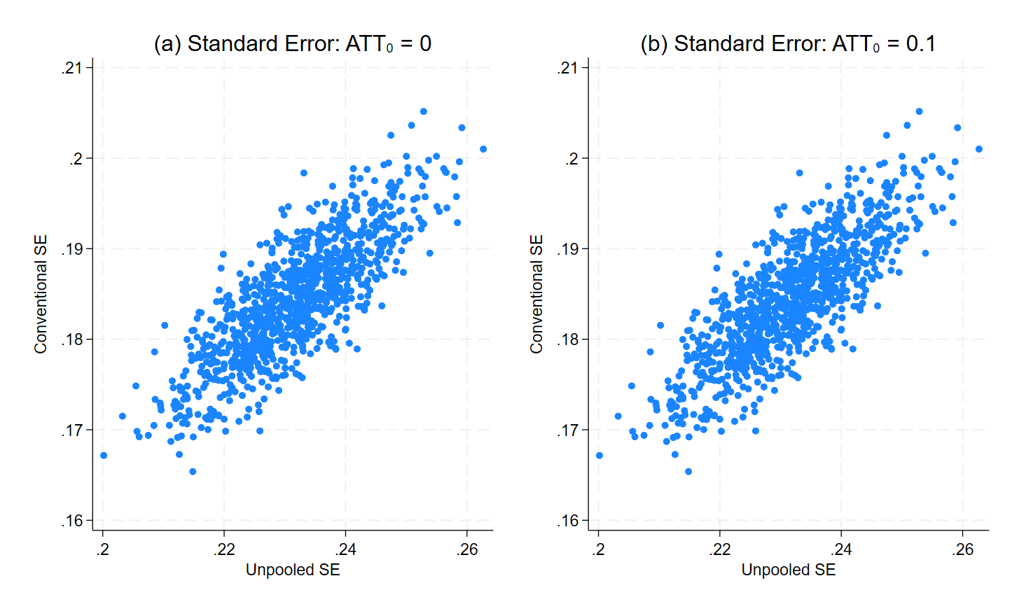
Figure 5: Time-Invariant Covariate with Equal Sample Sizes: Scatter Plots

We hypothesize that the standard errors are not numerically equivalent due to small sample sizes. To verify that the two methods converge to the true standard error as sample size increases, we repeat the simulation with sample sizes of 1,000, 2,000, 4,000, 8,000, 10,000, and 50,000 while maintaining equal sample sizes in both silos. We then compute the MSE for both the ATTs and their associated standard errors to look for evidence of convergence. The results are shown in Figure 6. The MSEs on the y-axis are plotted against the sample sizes on the x-axis. The MSE for both the ATT and the standard errors between the UN–DID and the true ATT is illustrated by the red line in Figure 6. On the same axis, we plot the MSE for both ATTs and their standard errors when comparing the conventional method to the true ATT (illustrated by the blue line in Figure 6). Finally, we also plot the MSE of both ATT and standard errors between the conventional and UN–DID methods (represented by the green line in Figure 6).

Figure 6 depicts the MSE of ATTs for Case 3 in Panel (a) and for Case 4 in Panel (b). Panels (c) and (d) showcase the MSE of standard errors for Case 3 and Case 4, respectively. We observe that both ATT and standard error MSEs decrease with larger sample sizes, confirming that both the conventional and UN–DID methods converge to the true values of both the ATT and the standard errors as sample size increases. Notably, the UN–DID standard errors consistently exhibit lower MSE than the conventional estimator, suggesting more reliable inference using the UN–DID method, especially with smaller sample sizes. The graph also illustrates a decreasing MSE between the conventional and UN–DID methods with increasing sample size, indicating convergence between the two estimators. A similar convergence is observed in a case with unequal sample sizes, as shown in Figure 7.

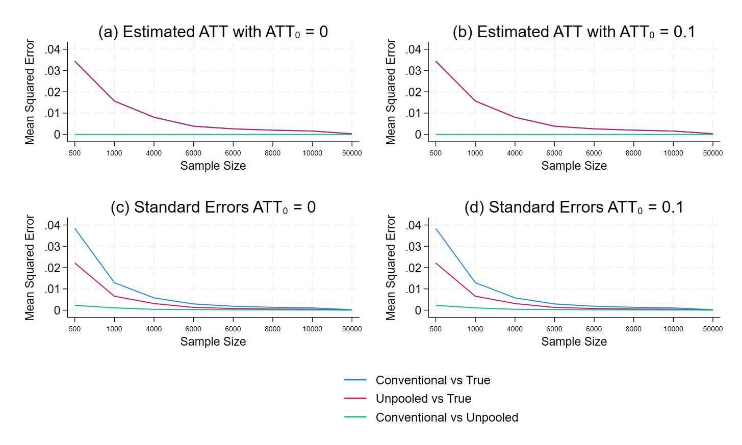
Figure 6: Time-Invariant Covariate with Equal Sample Sizes: Mean Squared Errors

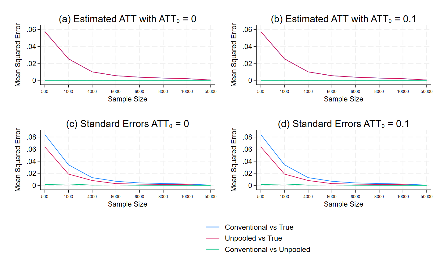
Figure 7: Time-Invariant Covariate with Unequal Sample Sizes: Mean Squared Errors

4.4 Monte Carlo Design with Time-Varying Covariates

In this section, we try to assess the performance of the UN–DID estimator with time-varying covariates. The Monte Carlo simulation design closely resembles the simulation of the previous subsection with a single time-invariant covariate. However, we replace the time-invariant covariate with a time-varying covariate, denoted by $X_{it}$. In our simulations, the time-varying covariate we used is age, which is unaffected by treatment even though it changes with time. Similar to the previous subsection, we analyze two cases where the true effect of the treatment is 0 and 0.1, respectively. A common slope parameter of 0.5 is assigned to the covariate in both the treated and the control silos. The DGPs for the two cases are as follows:

• Case 5: No treatment effect, time-varying covariate

  $$Y^{g}_{it}=0.5X^{g}_{it}+e^{g}_{it}.$$

• Case 6: Treatment effect, time-varying covariate

  $$Y^{g}_{it}=0.1*DID^{g}_{it}+0.5X^{g}_{it}+e^{g}_{it}.$$

4.5 Results: Time-Varying Covariate

In subsection 4.1, we have shown that both the conventional and UN–DID methods effectively identify the ATT in the presence of time-varying covariates with common slope parameters. However, it is worth noting that, while the estimates of ATT are close, they are not exactly numerically equal. However, with large sample sizes, the estimates get closer to the true value due to the law of large numbers. Therefore, the equivalence between the conventional and the UN–DID estimates holds only when we have a large enough sample size.

To assess the equivalence of ATT estimates and their associated standard errors, we created scatter plots, Figure 5. In Panel (a), we compare the conventional ATT (y-axis) with the UN–DID ATT (x-axis) for Case 5. Panel (b) shows a similar comparison for Case 6. Additionally, panels (c) and (d) illustrate the relationship between the conventional standard error (y-axis) and the UN–DID standard errors (x-axis) for cases 5 and 6, respectively. Upon inspecting the scatter plots, we observe that the points representing ATT estimates and their associated standard errors align along the $45^{\circ}$ line. However, they are not perfectly aligned, suggesting the estimates of ATT are not numerically equal but are equivalent. This pattern is consistent across both cases. We also find a similar trends when dealing with equal sample sizes (figures not shown).

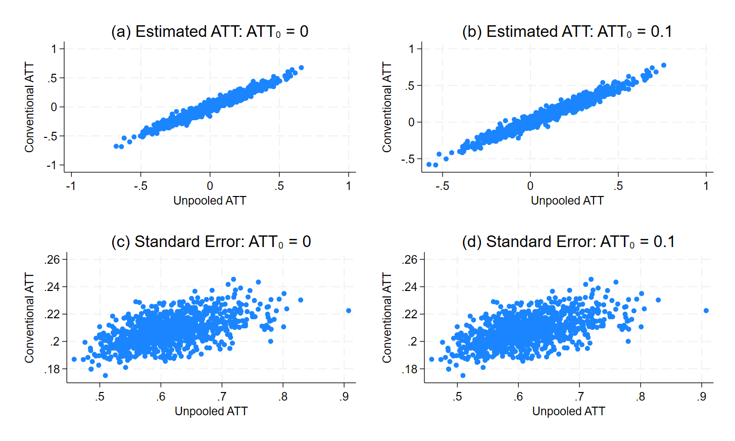
Figure 8: Time-Varying Covariate with Unequal Sample Sizes: Scatter Plots

Similar to the previous subsection, we assess the unbiasedness of the UN–DID estimator using kernel densities, illustrated in Figure 9. The kernel densities reveal that the distribution of ATTs is centered around the true ATT value, indicating unbiasedness with time-varying covariates (common). Compared with earlier figures, there are now some differences between the conventional and UN–DID ATTs.

Additionally, in Figure 10, we observe a decrease in MSE for both the conventional and UN–DID methods as sample size increases. This suggests that the ATT and the standard error between the two methods converge as sample size increases. The same patterns are observed for unequal sample sizes between silos, as shown in Figure 11. Interestingly, the standard errors seem to converge faster to the true values with the UN–DID estimator than they do with the conventional estimator when the silos are of unequal size.

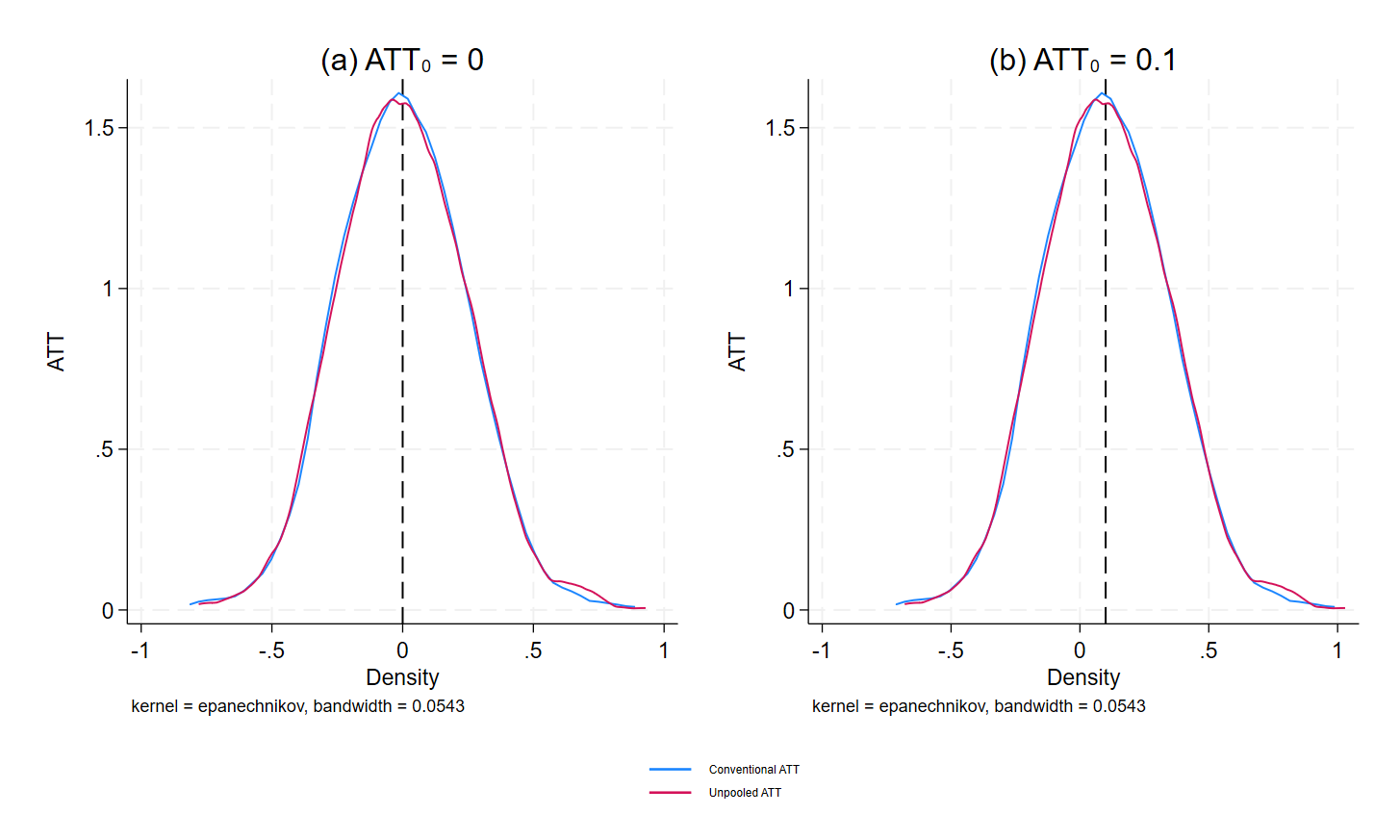
Figure 9: Time-Varying Covariates with Unequal Sample Sizes: Kernel Density

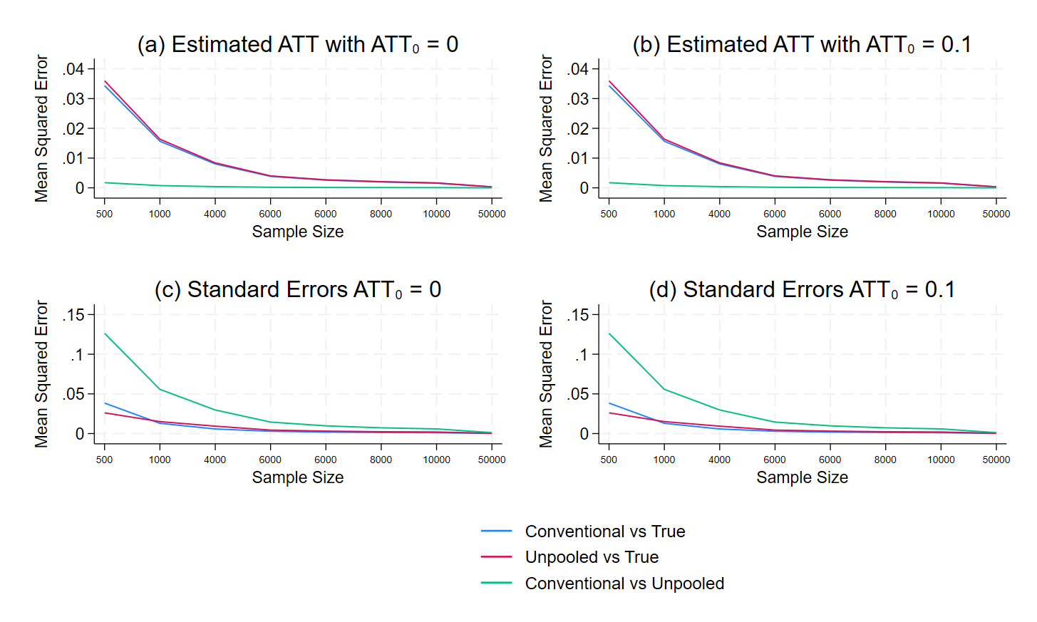
Figure 10: Time-Varying Covariate with Equal Sample Sizes: Mean Squared Errors

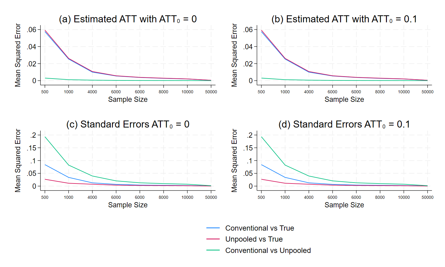
Figure 11: Time-Varying Covariate with Unequal Sample Sizes: Mean Squared Errors

4.6 Additional Types of Covariates

These simulations have considered only cases where we have a balanced panel. In practice, many researchers include covariates when they have access to repeated cross-sectional data. With repeated cross-sectional data, when binary or fixed effect-type coefficients are added, the equivalence of the estimated ATTs between UN–DID and conventional DID remains unchanged. The standard errors can be somewhat different. In this case, we recommend estimating

$$\equiv\;Y^{T}_{i,t}=\gamma_{0}^{T}+\gamma_{1}^{T}post_{t}^{T}+\gamma_{2}^{i}X^{T}_{i,t}+\nu^{T}_{i,t}$$ (53)

$$\equiv\;Y^{C}_{i,t}=\gamma_{0}^{C}+\gamma_{1}^{C}post_{t}^{C}+\gamma_{2}^{i}X^{C}_{i,t}+\nu^{C}_{i,t}$$ (54)

in place of the models without a constant. In this case, the ATT is just

$$\widehat{ATT}=\widehat{\gamma^{T}_{1}}-\widehat{\gamma^{C}_{1}}.$$ (55)

The equivalence between this specification and the regressions without a constant has been shown in Section 3.1. Additionally, the standard error is

$$\widehat{SE}(\widehat{ATT})=\sqrt{\widehat{SE}(\widehat{\gamma^{T}_{1}})^{2}+\widehat{SE}(\widehat{\gamma^{C}_{1}})^{2}}.$$ (56)

5 UN–DID with Staggered Adoption

In this section, we relax Assumption 5 to accommodate a scenario where multiple groups adopt treatment at different points in time, creating a staggered adoption framework. We also impose an additional restriction called absorptive state, which implies that, once a unit is treated, it remains treated for the rest of the period of the study. Similar to Callaway and Sant’Anna (2021), our proposed method will decompose the dataset into several $2\times 2$ group–time cells.

We will introduce some additional notation following Callaway and Sant’Anna (2021). Let $G_{i,g}=1$ if unit $i$ is treated at time $g$, and 0 otherwise. This will be referred to as the treatment start-time dummies. Following Callaway and Sant’Anna (2021), we group together each individual into $g\in G$ cohorts based on the treatment start-time dummies. For a particular group $g$, any period where $t<g$ are called pre-treatment periods. Under the no-anticipation assumption, the ATT(g,t) for pre-treatment periods are 0.

Each group–time cell contains a group that is currently treated and a group that has not yet been treated. The pre-intervention period in each $2\times 2$ cell is defined as the time period right before the treated group is treated ($g-1$). For each $2\times 2$ group–time cell, we will run the following two regressions:

$$\mbox{For treated:}\;Y^{T}_{i,t}=\zeta_{1}^{T}pre_{t}^{T}+\zeta_{2}^{T}post_{t}^{T}+\nu^{T}_{i,t}.$$ (57)

$$\mbox{For untreated:}\;Y^{C}_{i,t}=\zeta_{1}^{C}pre_{t}^{C}+\zeta_{2}^{C}post_{t}^{C}+\nu^{C}_{i,t}.$$ (58)

After these two regressions are estimated, the ATT(g,t) is

$$\widehat{ATT(g,t)}=(\zeta^{T}_{2}-\zeta^{T}_{1})-(\zeta^{C}_{2}-\zeta^{C}_{1}).$$ (59)

The above process is repeated for all relevant $2\times 2$ group–time cells. These ATT(g,t) cells will then be aggregated together to get an overall estimate of the ATT based on Equation (60). $w_{g,t}$ are the weights associated with each of the ATT(g,t) cells. Common weighting schemes include equal weighting for each cell and population-based weighting. Refer to Callaway and Sant’Anna (2021) and Xiong et al. (2023) for details.

$$\widehat{ATT}=\sum_{g=2}^{G}\sum_{t=2}^{\mathcal{T}}1\{g\leq t\}w_{g,t}ATT(g,t).$$ (60)

6 Empirical Examples

6.1 The Impact of Marijuana Legalization on Body Mass Index

We revisit the question asked in Sabia et al. (2017) to see how comparable the UN–DID estimates of an ATT may be in comparison to conventional methods. Specifically, we ask whether whether legalizing marijuana has any impact on body mass index (BMI).

We use data from the Behavioral Risk Factor Surveillance System. This repeated cross-section has records from people of all ages. However, we restrict our attention to those aged 25 or older. We use data from 2006–2013 from New York and the District of Columbia (DC). DC relaxed their marijuana laws in 2010. Thus we have a $2\times 8$ design with an equal number of pre-treatment and post-treatment years. There are 84,783 observations in the final sample.

With this data, we estimate four different treatment effects: from a conventional DID regression and with UN–DID, with and without controls. The control variables are female and categorical variables for age, race, and education. The conventional DID model we estimate is shown in Equation (61). We estimate the UN–DID ATT using the alternate specification given in equations (53) and (53).

$$\footnotesize\text{BMI}_{ist}=\beta_{0}+\beta_{1}\text{post}_{t}+\beta_{2}\text{treat}_{s}+\beta_{1}\text{did}_{st}+\delta_{1}\text{female}_{ist}+\delta_{2}\text{RACE}_{ist}+\delta_{3}\text{AGE}_{ist}+\delta_{4}\text{EDUC}_{ist}+\epsilon_{ist}.$$ (61)

Table 1 presents the estimates. As expected, without covariates, we get exactly the same coefficients from both the conventional and UN–DID estimates, with an estimated ATT of 0.2560 and a standard error of 0.0853. This suggests that there was a statistically significant increase in BMI after the legalization of marijuana, in contrast to the findings in Sabia et al. (2017).

When we add covariates, the estimated coefficient drops considerably, to 0.1322 for the conventional DID and to 0.1204 for UN–DID. Again, this difference between the two estimates is expected, especially because there are 25 covariates in the model. The standard errors are also slightly smaller, at 0.0807 for the conventional model and 0.0811 for UN–DID. The p-value for the conventional DID is just above the 10% threshold, at 0.102, suggesting marijuana legalization did not have a statistically significant impact on BMI.

Table 1: Effect of Marijuana Legalization on BMI

	Conventional	UN–DID	Conventional	UN–DID
Coefficient	0.2560	0.2560	0.1322	0.1204
Standard error	0.0853	0.0853	0.0807	0.0811
Covariates	No	No	Yes	Yes

6.2 The Impact of Merit Scholarships on College Attendance

To highlight the use of the new method proposed, we revisit the analysis of “merit scholarships.” These scholarships vary in their design, generally awarding scholarships to high achieving high school students to enroll in a college within their home state. See Deming and Dynarski (2010) and the references therein for a nice survey. We use the dataset analyzed as an empirical example in Conley and Taber (2011), which estimates the average impact of 10 different merit scholarship programs with different adoption dates.

Specifically, we estimate how the likelihood of an individual being a college graduate changes as a result of their home state adopting a merit scholarship program. We first estimate this effect individually for each of the 10 treated states. This allows us to compare 10 distinct estimates of treatment effects using both the UN–DID procedure and the the conventional procedure. There are 51 “states” (including DC) in the dataset and 12 years of data from 1989 to 2000. Across all states and years, there are 42,161 individual-level observations, representing a repeated cross-section.

Ten states in the sample adopt a merit scholarship, with adoption dates that vary greatly. Four states adopt the scholarship in 1991, 1993, 1996, and 1999, respectively, while two states each adopt the scholarship in years 1997, 1998, and 2000. For each treated state, a control state was chosen from the set of 41 untreated states. The control states were chosen to roughly match the number of treated and untreated observations in each model. We use only one treated state to highlight the properties of the UN–DID estimator rather than to estimate the best possible counterfactuals. We estimate the treatment effects both with and without covariates. Specifically, using only data from treated state $T$ and untreated state $U$, we estimate the model:

$$\text{college}_{ist}=\beta_{1}\text{post}_{t}+\beta_{2}\text{treat}_{s}+\beta_{1}\text{did}_{st}+\delta_{1}\text{black}_{ist}+\delta_{2}\text{asian}_{ist}+\delta_{3}\text{male}_{ist}+\epsilon_{ist}.$$ (62)

The coefficients $\delta_{1},\delta_{2}$, and $\delta_{3}$ are estimated only when the covariates are included. The remaining variables are defined the standard way: $treat_{s}$ is set equal to 1 for observations in state $T$ and is set equal to 0 for observations in state $U$. Similarly, $post_{t}$ is set equal to 1 for years greater than and equal to the year when state $T$ first offered a merit scholarship. Finally, $did_{st}$ is the product of $treat_{s}$ and $post_{t}$. We estimate all these treatment effects, or $\widehat{did}_{st}$, and their standard errors using both the pooled dataset and the UN–DID estimates and standard errors by artificially siloing the data.

The results of these estimates are found in Table 2. Panel A shows the estimates for the models without covariates. The first thing to notice is that the treatment effects are identical when we estimate using either the conventional method with the pooled data or the UN–DID method with the unpooled data. Additionally, the standard errors always agree to the third decimal place, and agree to the fourth decimal place in all but one of the estimates. These results match the simulation results presented in Section 3.3.

Panel B of Table 2 shows the estimates with covariates included. Here, some of the treatment effects are estimated to be very similar using either the conventional pooled approach or the UN–DID approach. For instance, for the treatment of state 88 versus state 11, the conventional estimate is 0.1811 and the UN–DID estimate is 0.1819. However, some of the estimates are not as close. The treatment effect of state 61 versus state 62 is estimated to be 0.0370 with the conventional approach and 0.0314 with the UN–DID approach. The estimates for the standard errors differ considerably more. These findings are consistent with the results in Section 4.4.

Additionally, we attempt to estimate a single treatment effect using data from all years and all groups. We do this using three methods, two with pooled data and one with unpooled data. The first pooled method estimates a two-way fixed effect (TWFE) difference-in-differences model, similar to Equation 62 but replacing the $treat_{s}$ and $post_{t}$ terms with state and year fixed effects. This replicates the original analysis in Conley and Taber (2011). Given the staggered adoption, the TWFE estimates contain “forbidden comparisons.” Accordingly, we also estimate the ATT using the CSDID command, which implements the Callaway and Sant’Anna (2021) procedure. Finally, we estimate the same ATT, using only the non-forbidden comparisons estimated with the UN–DID method by again pretending that each state’s data is siloed.

The aggregate ATT estimates are shown in Panel C of Table 2. With no covariates we find that all three estimates are quite similar. Specifically, the TWFE estimate is 0.0374, the CSDID estimate is 0.0339, and the UN–DID estimate is 0.0361. We do not expect the CSDID and UN–DID estimates to entirely agree, for two reasons. The first is that the CSDID estimate is doubly robust and the UN–DID estimate is not. The second is the “treatment unit” in CSDID is the year of adoption, whereas we regard the state as the “treatment unit” because that is the level of siloing of the data. With covariates, we see that the TWFE and CSDID estimates are very similar, at 0.0337 and 0.0339, respectively. The UN–DID estimate is slightly smaller at 0.0295. One reason for this difference is that the UN–DID approach in this case involves 51 separate regressions estimating 153 coefficients for the controls, whereas the pooled approaches need to estimate only three coefficients to handle the controls. Taken together, these estimates suggest that the UN–DID approach with unpooled data gives very similar estimates to conventional methods using pooled data.

Table 2: Estimates from Merit Example

Panel A: Without Covariates
Treated	Control	Year	Conventional	UN–DID	Conventional SE	UN–DID SE
71	73	1991	$-0$.0242	$-0$.0242	0.0755	0.0754
58	46	1993	0.1386	0.1386	0.0590	0.0590
64	54	1996	0.0182	0.0182	0.0619	0.0619
59	23	1997	$-0$.0073	$-0$.0073	0.0362	0.0362
85	86	1997	0.1318	0.1318	0.0601	0.0601
57	32	1998	$-0$.0291	$-0$.0291	0.0747	0.0747
72	55	1998	$-0$.0645	$-0$.0645	0.0658	0.0658
61	62	1999	0.0335	0.0335	0.0816	0.0816
34	33	2000	$-0$.0305	$-0$.0305	0.0666	0.0666
88	11	2000	0.1595	0.1595	0.1337	0.1337
Panel B: With Covariates
Treated	Control	Year	Conventional	UN–DID	Conventional SE	UN–DID SE
71	73	1991	$-0$.0141	$-0$.0137	0.0750	0.0871
58	46	1993	0.1501	0.1523	0.0582	0.0734
64	54	1996	0.0077	0.0028	0.0614	0.0820
59	23	1997	$-0$.0179	$-0$.0139	0.0360	0.0441
85	86	1997	0.1309	0.1277	0.0597	0.0726
57	32	1998	$-0$.0480	$-0$.0417	0.0733	0.0876
72	55	1998	$-0$.0704	$-0$.0685	0.0655	0.0793
61	62	1999	0.0370	0.0314	0.0806	0.0918
34	33	2000	$-0$.0282	$-0$.0303	0.0655	0.0709
88	11	2000	0.1811	0.1819	0.1335	0.1428
Panel C: Full Sample
Years	Covariates		UN–DID	TWFE	CSDID
All	No		0.0361	0.0374	0.0339
All	Yes		0.0295	0.0337	0.0339

7 Conclusion

In this paper, we propose an extension to the conventional regression-based method for difference-in-differences to settings with unpoolable data called UN–DID. Using simulations and analytical proofs, we show that the proposed method results in identical coefficients and standard errors to the conventional method with no covariates. We also show that it is unbiased. When time-invariant covariates are added, the coefficients can be the same as the conventional ones, but the standard errors differ. Time-varying covariates cause neither the coefficients nor the standard errors to be equal with small sample sizes but converge as sample size increases. We extend the UN–DID method to a setting with staggered adoption and verify the results from the simulation study and analytical proofs with an empirical example.

A Interpretation of the Coefficients in Equation (11)

To begin, let us rewrite Equation (11) and proceed to derive the values for $\alpha_{0}$, $\alpha_{1}$, and $\alpha_{2}$:

$$P_{t}*D_{i}=\alpha_{0}+\alpha_{1}P_{t}+\alpha_{2}D_{i}+u_{i,t}.$$ (A1)

With a constant, we prove that the coefficient of a dummy variable represents the difference in means when the dummy variable takes on a value of 1 compared to when it takes on a value of 0.

General Proof: Let $M$ be a continuous outcome variable and $N$ be a binary dummy variable. The regression of $M$ on $N$ is expressed as

$$M=\kappa_{0}+\kappa_{1}N+\upsilon.$$ (A2)

By taking expectations, once when $N=1$ and once when $N=0$, we obtain

$$E[M|N=1]=\kappa_{0}+\kappa_{1}$$ (A3)

$$\Rightarrow E[M|N=0]=\kappa_{0}.$$ (A4)

With strict exogeneity, we know that $E[\upsilon|N=1]=0$ and $E[\upsilon|N=0]=0$. By subtracting Equation (A4) from Equation (A3), it becomes evident that

$$\kappa_{1}=E[M|N=1]-E[M|N=0].$$ (A5)

Based on this proof, we can write $\alpha_{1}$ as

$$\alpha_{1}=E[P_{t}*D_{i}|D_{i}=1]-E[P_{t}*D_{i}|D_{i}=0].$$ (A6)

When $D_{i}=0$, $P_{t}*D_{i}=0$. Therefore, $E[P_{t}*D_{i}|D_{i}=0]=0$. So we can rewrite Equation (A6) as

$$\alpha_{1}=E[P_{t}*D_{i}|D_{i}=1]=E[P_{t}]=Pr(P_{t}).$$ (A7)

Because $P_{t}$ is a dummy variable, $E[P_{t}]$ is the fraction of individuals in the post-intervention period. We can similarly show that $\alpha_{2}=E[D_{i}]=Pr(D_{i})$. To derive $\alpha_{0}$, let us take the unconditional expectation of Equation (A1):

$$E(P_{t}*D_{i})=\alpha_{0}+\alpha_{1}\cdot E(D_{i})+\alpha_{2}\cdot E(P_{t})$$ (A8)

$$\Rightarrow Pr(P_{t})\cdot Pr(D_{i})=\alpha_{0}+Pr(P_{t})\cdot Pr(D_{i})+Pr(D_{i})\cdot Pr(P_{t}).$$ (A9)

This follows from the fact that the expected value of a dummy variable is the fraction of the total sample with the dummy variable value = 1. The proof is shown below. We have also shown in Equation (A7) that $\alpha_{1}=Pr(D_{i})$ and $\alpha_{2}=Pr(P_{t})$.

Proof: The expected value of a binary dummy variable $D_{i}$ is given by

$$E[D_{i}]=\frac{\sum_{i=1}^{n}D_{i}}{n}.$$ (A10)

Because $D_{i}$ can take only the value of 0 or 1, we can express it as the count of observations, where $D_{i}=1$:

$$E[D_{i}]=\frac{\sum_{i=1}^{n}D_{i}}{n}=\frac{\text{Number of observations where }D_{i}=1}{n}.$$ (A11)

The same holds for $E(P_{t})$. We can now re-arrange and simplify Equation (A9) as follows:

$$\alpha_{0}=-Pr(P_{t})\cdot Pr(D_{i}).$$ (A12)

In other words, $\alpha_{0}$ is minus the fraction of individuals with both $P_{t}=1$ and $D_{i}=1$, $\alpha_{1}$ is the fraction of individuals in the post-intervention period, and $\alpha_{2}$ is the fraction of individuals in the pre-intervention period.

With equal sample sizes, $Pr(P_{t})=Pr(D_{i})=1/2$. This follows from the fact that approximately half of the total observations are in the post-intervention period and approximately half of the observations are in the treated group. So, $\alpha_{1}=1/2$, $\alpha_{2}=1/2$, and $\alpha_{0}=-1/4$. Following this, the sum of squared residuals $A$ from Equation (14) can be expressed as

$$A=\sum_{i\in t=0,T}\left(1/4-1/2\right)^{2}+\sum_{i\in t=1,T}\left(1+1/4-1/2-1/2\right)^{2}+\sum_{i\in t=0,C}\left(-1/4\right)^{2}+\sum_{i\in t=1,C}\left(1/4-1/2\right)^{2}$$

$$\Rightarrow A=N/16,\;\;\;\mbox{where N is the total sample size}.$$

Using the same values, we can show that $\left(1-\hat{\alpha}_{0}-\hat{\alpha}_{1}-\hat{\alpha}_{2}\right)=\left(\hat{\alpha}_{0}+\hat{\alpha}_{2}\right)=\left(\hat{\alpha}_{0}+\hat{\alpha}_{2}\right)=\left(-\hat{\alpha}_{0}\right)=1/4$ from Equation (39). Therefore, we can show that $\frac{\left(1-\hat{\alpha}_{0}-\hat{\alpha}_{1}-\hat{\alpha}_{2}\right)}{A}=\frac{\left(\hat{\alpha}_{0}+\hat{\alpha}_{2}\right)}{A}=\frac{\left(\hat{\alpha}_{0}+\hat{\alpha}_{2}\right)}{A}=\frac{\left(-\hat{\alpha}_{0}\right)}{A}=1/(N/4)$. With equal sample sizes, $N_{1,1}=N_{0,1}=N_{1,0}=N_{0,0}=N/4$.

Following this, we can conclude that $\frac{\left(1-\hat{\alpha}_{0}-\hat{\alpha}_{1}-\hat{\alpha}_{2}\right)}{A}$ is the reciprocal of the number of observations in the treated group and the post-intervention period ($N_{1,1})$ and $\frac{\left(\hat{\alpha}_{0}+\hat{\alpha}_{2}\right)}{A}$ is the reciprocal of the number of observations in the treated group in the pre-intervention period ($N_{1,0}$). Similarly, $\frac{\left(\hat{\alpha}_{0}+\hat{\alpha}_{2}\right)}{A}$ is the reciprocal of the number of observations in the control group in the post-intervention period $(N_{0,1})$, and $\frac{\left(-\hat{\alpha}_{0}\right)}{A}$ is reciprocal of the number of observations in the control group in the pre-intervention period ($N_{0,0})$. The same results hold for cases with unequal sample sizes.

With time-varying covariates, $\alpha_{3}$ is interpreted as $Pr(X_{i,t})=x$. Therefore, $\frac{\left(1-\hat{\alpha}_{0}-\hat{\alpha}_{1}-\hat{\alpha}_{2}-\hat{\alpha}_{3}x\right)}{G^{\prime}}$ and $\frac{\left(\hat{\alpha}_{0}+\hat{\alpha}_{2}+\hat{\alpha}_{3}x\right)}{G^{\prime}}$ are equivalent to the reciprocals of the number of observations in the treated group in the post-intervention period and the pre-intervention period, respectively, with $X_{i,t}=x$. Similarly, $\frac{\left(\hat{\alpha}_{0}+\hat{\alpha}_{1}+\hat{\alpha}_{3}x\right)}{G^{\prime}}$ and $\frac{\left(-\hat{\alpha}_{0}-\hat{\alpha}_{3}x\right)}{G^{\prime}}$ represent the probabilities for the observations being in the control group in the post- and pre-intervention periods, respectively, conditional on $X_{i,t}$.

References

- Abadie (2005) Abadie, A. (2005) “Semiparametric difference-in-differences estimators,” The review of economic studies 72(1), 1–19
- Bernal et al. (2017) Bernal, J. L., S. Cummins, and A. Gasparrini (2017) “Interrupted time series regression for the evaluation of public health interventions: a tutorial,” International journal of epidemiology 46(1), 348–355
- Bertrand et al. (2004) Bertrand, M., E. Duflo, and S. Mullainathan (2004) “How much should we trust differences-in-differences estimates?,” The Quarterly journal of economics 119(1), 249–275
- Caetano et al. (2022) Caetano, C., B. Callaway, S. Payne, and H. S. Rodrigues (2022) “Difference in differences with time-varying covariates,” arXiv preprint arXiv:2202.02903
- Callaway and Sant’Anna (2021) Callaway, B., and P. H. Sant’Anna (2021) “Difference-in-differences with multiple time periods,” Journal of Econometrics 225(2), 200–230
- Card and Krueger (1993) Card, D., and A. B. Krueger (1993) “Minimum wages and employment: A case study of the fast food industry in new jersey and pennsylvania,”
- Conley and Taber (2011) Conley, T. G., and C. R. Taber (2011) “Inference with “difference in differences” with a small number of policy changes,” The Review of Economics and Statistics 93(1), 113–125
- De Chaisemartin and d’Haultfoeuille (2020a) De Chaisemartin, C., and X. d’Haultfoeuille (2020a) “Two-way fixed effects estimators with heterogeneous treatment effects,” American Economic Review 110(9), 2964–2996
- Deming and Dynarski (2010) Deming, D., and S. Dynarski (2010) “College aid,” in Targeting investments in children: Fighting poverty when resources are limited, pp. 283–302, University of Chicago Press
- Hallock et al. (2021) Hallock, H., S. E. Marshall, P. A. t Hoen, J. F. Nygård, B. Hoorne, C. Fox, and S. Alagaratnam (2021) “Federated networks for distributed analysis of health data,” Frontiers in Public Health 9, 712569
- Heckman et al. (1997) Heckman, J. J., H. Ichimura, and P. E. Todd (1997) “Matching as an econometric evaluation estimator: Evidence from evaluating a job training programme,” The review of economic studies 64(4), 605–654
- Li et al. (2022) Li, Q., Y. Diao, Q. Chen, and B. He (2022) “Federated learning on non-iid data silos: An experimental study,” in 2022 IEEE 38th International Conference on Data Engineering (ICDE), pp. 965–978, IEEE
- Masten and Poirier (2018) Masten, M. A., and A. Poirier (2018) “Identification of treatment effects under conditional partial independence,” Econometrica 86(1), 317–351
- McCullough (2008) McCullough, J. S. (2008) “The adoption of hospital information systems,” Health economics 17(5), 649–664
- Miller and Tucker (2014) Miller, A. R., and C. Tucker (2014) “Health information exchange, system size and information silos,” Journal of health economics 33, 28–42
- Roth et al. (2022) Roth, J., P. H. Sant’Anna, A. Bilinski, and J. Poe (2022) “What’s trending in difference-in-differences? a synthesis of the recent econometrics literature,” arXiv preprint arXiv:2201.01194
- Sabia et al. (2017) Sabia, J. J., J. Swigert, and T. Young (2017) “The effect of medical marijuana laws on body weight,” Health economics 26(1), 6–34
- Sant’Anna and Zhao (2020) Sant’Anna, P. H., and J. Zhao (2020) “Doubly robust difference-in-differences estimators,” Journal of Econometrics 219(1), 101–122
- Wang and Alexander (2020) Wang, L., and C. A. Alexander (2020) “Big data analytics in medical engineering and healthcare: methods, advances and challenges,” Journal of medical engineering & technology 44(6), 267–283
- Xiong et al. (2023) Xiong, R., A. Koenecke, M. Powell, Z. Shen, J. T. Vogelstein, and S. Athey (2023) “Federated causal inference in heterogeneous observational data,” Statistics in Medicine 42(24), 4418–4439