Fock-space relativistic coupled-cluster calculations of clock transition properties in Pb²⁺

Abstract

We have employed an all-particle Fock-space relativistic coupled-cluster theory to probe $6s^{2}{\;{}^{1}}S_{0}-6s6p{\;{}^{3}P^{o}_{0}}$ clock transition in an even isotope of Pb²⁺. We have computed the excitation energies for several low lying states, E1 and M1 transition amplitudes, and the lifetime of the clock state. Moreover, we have also calculated the electric dipole polarizability of the ground state using perturbed relativistic coupled-cluster theory. To improve the accuracy of results, we incorporated the corrections from the relativistic and QED effects in all our calculations. Contributions from the triple excitations are accounted perturbatively. Our computed excitation energies are in excellent agreement with the experimental values for all states. Our computed lifetime, $10.45\times 10^{6}$ s, of clock state is $\approx$ 16% larger than the previously reported value using CI+MBPT [Phys. Rev. Lett. 127, 013201 (2021)]. Based on our analysis, we find that the contributions from the valence-valence electron correlations from higher energy configurations and the corrections from the perturbative triples and QED effects are essential to get accurate clock properties in Pb²⁺. Our computed value of dipole polarizability is in good agreement with the available theory and experimental data.

I Introduction

Optical atomic clocks are one of the most accurate time measurement instruments in existence today Ludlow et al. (2015); De and Sharma (2023). Due to their unprecedented accuracies as frequency and time standards, they can be used as important probes to several fundamental and technological applications. Some examples where atomic clocks are of vital importance include, the variation in the fundamental constants Safronova (2019); Prestage et al. (1995); Karshenboim and Peik (2010), probing physics beyond the standard model of particle physics Dzuba et al. (2018); Berengut et al. (2018), navigation systems Grewal et al. (2013); Major (2013), quantum computer Weiss and Saffman (2017); Wineland et al. (2002), the basis for redefining the second Karshenboim and Peik (2010); Riehle et al. (2018), and more Ludlow et al. (2015); De and Sharma (2023). For single ion optical clocks, the hyperfine induced $3s^{2}{\;{}^{1}}S_{0}-3s3p{\;{}^{3}}P^{o}_{0}$ (267.4 nm) transition based ²⁷Al⁺ is demonstrated to be one of the best clocks, with a fractional frequency uncertainty of $9.4\times 10^{-19}$ Brewer et al. (2019). The high accuracy in ²⁷Al⁺ could be attributed to the low sensitivity to electromagnetic fields, narrow natural linewidth and small room temperature black-body radiation (BBR) shift in the clock transition frequency Kállay et al. (2011); Safronova et al. (2011); Kumar et al. (2021a). Among the neutral atoms, a lattice clock based on degenerate fermionic ⁸⁷Sr atoms with a hyperfine-induced $5s^{2}{\;{}^{1}}S_{0}-5s5p{\;{}^{3}}P^{o}_{0}$ (698 nm) transition is reported to be one of the best neutral atoms’ clocks. The smallest fractional frequency error achieved is $\approx$ 2.0 $\times$ 10^-18 Nicholson et al. (2015); Bothwell et al. (2019).

In the search for achieving a new and improved frequency standard, an optical clock based on 6s${}^{2}{\;{}^{1}S_{0}}-6s6p{\;{}^{3}}P^{o}_{0}$ transition, mediated through a two photon E1+M1 channel, in doubly ionized even isotope of lead could be a promising candidate. Like the case of ²⁷Al⁺, the clock transition is an electric dipole forbidden transition between two $J=0$ states, providing a strong resistance to the environmental perturbations. In addition, unlike ²⁷Al⁺, the nuclear spin quantum number $I$ is zero. This is crucial, as it prevents clock transition from the nonscalar perturbations which may arise though the coupling of electrons’ and nuclear multipole moments. Despite this important prospect with lead for an accurate optical atomic clock, the clock transition properties are not well explored. For instance, in terms of theory calculations, to the best of our knowledge, there is only one study on the lifetime of the clock state Beloy (2021). The work Beloy (2021), employing a combined method of configuration interaction (CI) and many-body perturbation theory (MBPT), has computed the lifetime of clock state, ${\;{}^{3}}P^{o}_{0}$, as $9.0\times 10^{6}$ s. Considering there are no experimental inputs, more theory calculations, specially using the accurate methods like relativistic coupled-cluster (RCC), would be crucial to get more accurate insights into the clock properties. Moreover, the inclusion of relativistic and QED corrections to the properties calculations are must to get reliable results. It can thus be concluded that there is a clear research gap in terms of the scarcity of accurate properties results for ${}^{1}S_{0}-{{}^{3}}P^{o}_{0}$ clock transition in doubly ionized lead.

In this work, we have employed an all-particle multireference Fock-space relativistic coupled-cluster (FSRCC) theory to accurately examine the clock transition properties in Pb²⁺. It is to be noted that, RCC theory is one of the most reliable many-body theories for atomic structure calculations. It accounts for electron correlation effects to all-orders of residual Coulomb interaction and has been employed to obtain accurate properties results in several closed-shell and one-valence atoms and ions Pal et al. (2007); Mani et al. (2009); Nataraj et al. (2011); Kumar et al. (2020). The application of RCC for two-valence atomic systems, as the present case of Pb²⁺ clock transition, is, however, limited to few studies Eliav et al. (1995a, b); Mani and Angom (2011). And, the reason for this, perhaps, is the complications associated with the implementation of FSRCC theory for multi-reference systems Eliav et al. (1995a, b); Mani and Angom (2011); Kumar et al. (2021a). To address the clock transition properties in a comprehensive way, using FSRCC theory Mani and Angom (2011); Kumar et al. (2021a), we carried out precise calculations of the excitation energies and E1 and M1 transition amplitudes associated with ${}^{1}S_{0}-{{}^{3}}P^{o}_{0}$ transition in Pb²⁺. Using these results, we have then calculated the lifetime of the ${}^{3}P^{o}_{0}$ clock state. In addition, as electric dipole polarizability is a crucial parameter for estimating BBR shift in clock frequency, we have also calculated the ground state polarizability of Pb²⁺ using perturbed relativistic coupled-cluster (PRCC) theory Kumar et al. (2020, 2021b). Moreover, in all these properties calculations, we have incorporated and analyzed the contributions from the Breit interaction, QED corrections and perturbative triples.

The remainder of the paper is organized into five sections. In Sec. II, we provide a brief description of the FSRCC theory for two-valence atomic systems. We have given the coupled-cluster working equation for two-valence systems. In Sec. III, we provide and discuss the expression for E1M1 decay rate. The results obtained from our calculations are presented and analyzed in Sec. IV. Theoretical uncertainty in our computed results is discussed in Sec. V of the paper. Unless stated otherwise, all results and equations presented in this paper are in atomic units ( $\hbar=m_{e}=e=1/4\pi\epsilon_{0}=1$).

II Two-valence FSRCC Theory

As the clock transition involves atomic state functions (ASFs) of two-valence nature, we need an accurate multireference theory to calculate these wavefunctions and corresponding many-body energies. For this, in the present work, we have employed a FSRCC theory for two-valence, developed and reported in our previous works Mani and Angom (2011); Kumar et al. (2021a). In Refs. Mani and Angom (2011); Mani et al. (2017); Kumar et al. (2021a), we have discussed in detail the implementation of FSRCC theory in the form of sophisticated parallel codes and have also given the working equations and Goldstone diagrams contributing to the theory. So, here, for completeness, we provide a very brief description of FSRCC theory for two-valence atoms and properties calculations using it in the context of Pb²⁺.

The atomic state function for a two-valence atom or ion is obtained by solving the many-body Schrodinger equation

$$H^{\rm DCB}|\Psi_{vw}\rangle=E_{vw}|\Psi_{vw}\rangle,$$ (1)

where $|\Psi_{vw}\rangle$ is the exact many-body wavefunction and $E_{vw}$ is the corresponding exact energy. The indices $v,w,\cdots$ represent the valence orbitals. $H^{\rm DCB}$ is the Dirac-Coulomb-Breit no-virtual-pair Hamiltonian used in all calculations, and expressed as

$$H^{\rm DCB} = \sum_{i=1}^{N}\left[c\bm{\alpha}_{i}\cdot\mathbf{p}_{i}+(\beta_{i}-1)c^{2}-V_{N}(r_{i})\right]$$ (2)

$$+\sum_{i<j}\left[\frac{1}{r_{ij}}+g^{\rm B}(r_{ij})\right],$$

where $\bm{\alpha}$ and $\beta$ are the Dirac matrices, and $1/r_{ij}$ and $g^{\rm B}(r_{ij})$ are the Coulomb and Breit interactions, respectively. In FSRCC theory, $|\Psi_{vw}\rangle$ is written as

$$|\Psi_{vw}\rangle=e^{T}\left[1+S_{1}+S_{2}+\frac{1}{2}\left({S_{1}}^{2}+{S_{2}}^{2}\right)+R_{2}\right]|\Phi_{vw}\rangle,$$ (3)

where $|\Phi_{vw}\rangle,=a^{\dagger}_{w}a^{\dagger}_{v}|\Phi_{0}\rangle,$ is the Dirac-Fock reference state for a two-valence system. Operators $T$, $S$ and $R$ are the electron excitation operators, referred to as the coupled-cluster (CC) operators, for closed-shell, one-valence and two-valence sectors, respectively. The subscripts $1$ and $2$ with these operators represent the single and double excitations, referred to as the coupled-cluster with singles and doubles (CCSD) approximation. The FSRCC theory with CCSD approximation subsumes most of the electron correlation effects in atomic structure calculations and provides an accurate description of the atomic properties. In the second quantized representation, the CC operators can be expressed as

$$T_{1}=\sum_{ap}t_{a}^{p}a_{p}^{\dagger}a_{a}{\;\;\rm and\;\;}T_{2}=\frac{1}{2!}\sum_{abpq}t_{ab}^{pq}a_{p}^{\dagger}a_{q}^{\dagger}a_{b}a_{a},$$ (4a)

$$S_{1}=\sum_{p}s_{v}^{p}a_{p}^{\dagger}a_{v}{\;\;\rm and\;\;}S_{2}=\sum_{apq}s_{va}^{pq}a_{p}^{\dagger}a_{q}^{\dagger}a_{a}a_{v},$$ (4b)

$$R_{2}=\sum_{pq}r_{vw}^{pq}a_{p}^{\dagger}a_{q}^{\dagger}a_{w}a_{v}.$$ (4c)

Here, the indices $a,b,\ldots$ and $p,q,\ldots$ represent the core and virtual orbitals, respectively. And, $t_{\ldots}^{\ldots}$, $s_{\ldots}^{\ldots}$ and $r_{\ldots}^{\ldots}$ are the cluster amplitudes corresponding to $T$, $S$ and $R$ CC operators, respectively. The diagrammatic representation of these operators is shown in Fig. 1. It is to be mentioned that the dominant contributions from triple excitations are, however, also included in the present work using perturbative triples approach Kumar et al. (2021a).

Figure 1: The diagrammatic representation of closed-shell, one-valence and two-valence single and double CC operators.

The operators for closed-shell and one-valence sectors are obtained by solving the set of coupled nonlinear equations discussed in Refs. Mani et al. (2009) and Mani and Angom (2010), respectively. The two-valence CC operator, $R_{2}$, is obtained by solving the CC equation Mani and Angom (2011); Kumar et al. (2021a)

$$\langle\Phi^{pq}_{vw}|\bar{H}_{\rm N}+\{\mathchoice{\vbox{\hbox to0.0pt{\kern 5.00002pt\kern 4.56248pt\hbox{\vrule width=0.50003pt,height=0.0pt,depth=4.30554pt\vrule width=12.11664pt,height=0.0pt,depth=0.50003pt\vrule width=0.50003pt,height=0.0pt,depth=4.30554pt}\hss}\vskip 2.15277pt\vskip 6.83331pt}}{\vbox{\hbox to0.0pt{\kern 5.00002pt\kern 4.56248pt\hbox{\vrule width=0.50003pt,height=0.0pt,depth=4.30554pt\vrule width=12.11664pt,height=0.0pt,depth=0.50003pt\vrule width=0.50003pt,height=0.0pt,depth=4.30554pt}\hss}\vskip 2.15277pt\vskip 6.83331pt}}{\vbox{\hbox to0.0pt{\kern 5.00002pt\kern 3.19374pt\hbox{\vrule width=0.50003pt,height=0.0pt,depth=4.30554pt\vrule width=8.54164pt,height=0.0pt,depth=0.50003pt\vrule width=0.50003pt,height=0.0pt,depth=4.30554pt}\hss}\vskip 2.15277pt\vskip 4.78333pt}}{\vbox{\hbox to0.0pt{\kern 5.00002pt\kern 2.28123pt\hbox{\vrule width=0.50003pt,height=0.0pt,depth=4.30554pt\vrule width=6.95831pt,height=0.0pt,depth=0.50003pt\vrule width=0.50003pt,height=0.0pt,depth=4.30554pt}\hss}\vskip 2.15277pt\vskip 3.41666pt}}\bar{H}_{\rm N}S^{{}^{\prime}}\}+\{\mathchoice{\vbox{\hbox to0.0pt{\kern 5.00002pt\kern 4.56248pt\hbox{\vrule width=0.50003pt,height=0.0pt,depth=4.30554pt\vrule width=12.11664pt,height=0.0pt,depth=0.50003pt\vrule width=0.50003pt,height=0.0pt,depth=4.30554pt}\hss}\vskip 2.15277pt\vskip 6.83331pt}}{\vbox{\hbox to0.0pt{\kern 5.00002pt\kern 4.56248pt\hbox{\vrule width=0.50003pt,height=0.0pt,depth=4.30554pt\vrule width=12.11664pt,height=0.0pt,depth=0.50003pt\vrule width=0.50003pt,height=0.0pt,depth=4.30554pt}\hss}\vskip 2.15277pt\vskip 6.83331pt}}{\vbox{\hbox to0.0pt{\kern 5.00002pt\kern 3.19374pt\hbox{\vrule width=0.50003pt,height=0.0pt,depth=4.30554pt\vrule width=8.54164pt,height=0.0pt,depth=0.50003pt\vrule width=0.50003pt,height=0.0pt,depth=4.30554pt}\hss}\vskip 2.15277pt\vskip 4.78333pt}}{\vbox{\hbox to0.0pt{\kern 5.00002pt\kern 2.28123pt\hbox{\vrule width=0.50003pt,height=0.0pt,depth=4.30554pt\vrule width=6.95831pt,height=0.0pt,depth=0.50003pt\vrule width=0.50003pt,height=0.0pt,depth=4.30554pt}\hss}\vskip 2.15277pt\vskip 3.41666pt}}\bar{H}_{\rm N}R_{2}\}|\Phi_{vw}\rangle=$$

$$E^{\rm att}_{vw}\langle\Phi^{pq}_{vw}|\Bigl{[}S^{{}^{\prime}}+R_{2}\Bigr{]}|\Phi_{vw}\rangle.$$ (5)

Here, for compact notation we have used $S^{\prime}=S_{1}+S_{2}+\frac{1}{2}(S^{2}_{1}+S^{2}_{2})$. $E^{\rm att}_{vw}$ is the two-electron attachment energy and it is expressed as the difference between the correlated energy of $(n-2)-$electron (closed-shell) and $n-$electron (two-valence) sectors, $E_{vw}-E_{0}$.

Figure 2: The CC diagrams contributing to the linearized FSRCC theory for two-valence atomic systems. Diagrams (l) - (n) are referred to as the folded diagrams and arise from the renormalization terms in CC equations for multireference systems.

In Fig. 2, we have given the Goldstone diagrams contributing to linearized FSRCC theory for two-valence systems. These are obtained by considering the terms with only one order of CC operators in Eq. (5) and then contracting residual Coulomb interaction with these CC operators using Wick’s theorem. The CC diagrams $(l)-(n)$ are referred to as the folded diagrams and they arise due to renormalization terms on the right hand side of Eq. (5). The presence of folded diagrams in open-shell systems constitute one of the main differences from the CC theory of closed-shell systems. The rectangular portion represents the effective energy diagrams arising from the one-valence (diagram (l)) and two-valence (diagrams (m) and (n)) sectors. The Goldstone diagrams in Fig. 2 correspond to the algebraic expression

$$\langle H_{\rm N} \rangle^{pq}_{vw}+\langle\mathchoice{\vbox{\hbox to0.0pt{\kern 0.0pt\kern 4.56248pt\hbox{\vrule width=0.50003pt,height=0.0pt,depth=4.30554pt\vrule width=12.3788pt,height=0.0pt,depth=0.50003pt\vrule width=0.50003pt,height=0.0pt,depth=4.30554pt}\hss}\vskip 2.15277pt\vskip 6.83331pt}}{\vbox{\hbox to0.0pt{\kern 0.0pt\kern 4.56248pt\hbox{\vrule width=0.50003pt,height=0.0pt,depth=4.30554pt\vrule width=12.3788pt,height=0.0pt,depth=0.50003pt\vrule width=0.50003pt,height=0.0pt,depth=4.30554pt}\hss}\vskip 2.15277pt\vskip 6.83331pt}}{\vbox{\hbox to0.0pt{\kern 0.0pt\kern 3.19374pt\hbox{\vrule width=0.50003pt,height=0.0pt,depth=4.30554pt\vrule width=8.72516pt,height=0.0pt,depth=0.50003pt\vrule width=0.50003pt,height=0.0pt,depth=4.30554pt}\hss}\vskip 2.15277pt\vskip 4.78333pt}}{\vbox{\hbox to0.0pt{\kern 0.0pt\kern 2.28123pt\hbox{\vrule width=0.50003pt,height=0.0pt,depth=4.30554pt\vrule width=7.0894pt,height=0.0pt,depth=0.50003pt\vrule width=0.50003pt,height=0.0pt,depth=4.30554pt}\hss}\vskip 2.15277pt\vskip 3.41666pt}}H_{\rm N}T\rangle^{pq}_{vw}+\langle\mathchoice{\vbox{\hbox to0.0pt{\kern 0.0pt\kern 4.56248pt\hbox{\vrule width=0.50003pt,height=0.0pt,depth=4.30554pt\vrule width=12.11664pt,height=0.0pt,depth=0.50003pt\vrule width=0.50003pt,height=0.0pt,depth=4.30554pt}\hss}\vskip 2.15277pt\vskip 6.83331pt}}{\vbox{\hbox to0.0pt{\kern 0.0pt\kern 4.56248pt\hbox{\vrule width=0.50003pt,height=0.0pt,depth=4.30554pt\vrule width=12.11664pt,height=0.0pt,depth=0.50003pt\vrule width=0.50003pt,height=0.0pt,depth=4.30554pt}\hss}\vskip 2.15277pt\vskip 6.83331pt}}{\vbox{\hbox to0.0pt{\kern 0.0pt\kern 3.19374pt\hbox{\vrule width=0.50003pt,height=0.0pt,depth=4.30554pt\vrule width=8.54164pt,height=0.0pt,depth=0.50003pt\vrule width=0.50003pt,height=0.0pt,depth=4.30554pt}\hss}\vskip 2.15277pt\vskip 4.78333pt}}{\vbox{\hbox to0.0pt{\kern 0.0pt\kern 2.28123pt\hbox{\vrule width=0.50003pt,height=0.0pt,depth=4.30554pt\vrule width=6.95831pt,height=0.0pt,depth=0.50003pt\vrule width=0.50003pt,height=0.0pt,depth=4.30554pt}\hss}\vskip 2.15277pt\vskip 3.41666pt}}H_{\rm N}S^{{}^{\prime}}\rangle^{pq}_{vw}+\langle\mathchoice{\vbox{\hbox to0.0pt{\kern 0.0pt\kern 4.56248pt\hbox{\vrule width=0.50003pt,height=0.0pt,depth=4.30554pt\vrule width=12.11664pt,height=0.0pt,depth=0.50003pt\vrule width=0.50003pt,height=0.0pt,depth=4.30554pt}\hss}\vskip 2.15277pt\vskip 6.83331pt}}{\vbox{\hbox to0.0pt{\kern 0.0pt\kern 4.56248pt\hbox{\vrule width=0.50003pt,height=0.0pt,depth=4.30554pt\vrule width=12.11664pt,height=0.0pt,depth=0.50003pt\vrule width=0.50003pt,height=0.0pt,depth=4.30554pt}\hss}\vskip 2.15277pt\vskip 6.83331pt}}{\vbox{\hbox to0.0pt{\kern 0.0pt\kern 3.19374pt\hbox{\vrule width=0.50003pt,height=0.0pt,depth=4.30554pt\vrule width=8.54164pt,height=0.0pt,depth=0.50003pt\vrule width=0.50003pt,height=0.0pt,depth=4.30554pt}\hss}\vskip 2.15277pt\vskip 4.78333pt}}{\vbox{\hbox to0.0pt{\kern 0.0pt\kern 2.28123pt\hbox{\vrule width=0.50003pt,height=0.0pt,depth=4.30554pt\vrule width=6.95831pt,height=0.0pt,depth=0.50003pt\vrule width=0.50003pt,height=0.0pt,depth=4.30554pt}\hss}\vskip 2.15277pt\vskip 3.41666pt}}H_{\rm N}R_{2}\rangle^{pq}_{vw}-$$ (6)

$$\langle\mathchoice{\vbox{\hbox to0.0pt{\kern 0.0pt\kern 3.97916pt\hbox{\vrule width=0.50003pt,height=0.0pt,depth=4.30554pt\vrule width=15.11388pt,height=0.0pt,depth=0.50003pt\vrule width=0.50003pt,height=0.0pt,depth=4.30554pt}\hss}\vskip 2.15277pt\vskip 6.83331pt}}{\vbox{\hbox to0.0pt{\kern 0.0pt\kern 3.97916pt\hbox{\vrule width=0.50003pt,height=0.0pt,depth=4.30554pt\vrule width=15.11388pt,height=0.0pt,depth=0.50003pt\vrule width=0.50003pt,height=0.0pt,depth=4.30554pt}\hss}\vskip 2.15277pt\vskip 6.83331pt}}{\vbox{\hbox to0.0pt{\kern 0.0pt\kern 2.7854pt\hbox{\vrule width=0.50003pt,height=0.0pt,depth=4.30554pt\vrule width=10.68193pt,height=0.0pt,depth=0.50003pt\vrule width=0.50003pt,height=0.0pt,depth=4.30554pt}\hss}\vskip 2.15277pt\vskip 4.78333pt}}{\vbox{\hbox to0.0pt{\kern 0.0pt\kern 1.98956pt\hbox{\vrule width=0.50003pt,height=0.0pt,depth=4.30554pt\vrule width=9.09026pt,height=0.0pt,depth=0.50003pt\vrule width=0.50003pt,height=0.0pt,depth=4.30554pt}\hss}\vskip 2.15277pt\vskip 3.41666pt}}E^{\rm att}_{vw}S^{{}^{\prime}}\rangle^{pq}_{vw}-\langle\mathchoice{\vbox{\hbox to0.0pt{\kern 0.0pt\kern 3.97916pt\hbox{\vrule width=0.50003pt,height=0.0pt,depth=4.30554pt\vrule width=14.96979pt,height=0.0pt,depth=0.50003pt\vrule width=0.50003pt,height=0.0pt,depth=4.30554pt}\hss}\vskip 2.15277pt\vskip 6.83331pt}}{\vbox{\hbox to0.0pt{\kern 0.0pt\kern 3.97916pt\hbox{\vrule width=0.50003pt,height=0.0pt,depth=4.30554pt\vrule width=14.96979pt,height=0.0pt,depth=0.50003pt\vrule width=0.50003pt,height=0.0pt,depth=4.30554pt}\hss}\vskip 2.15277pt\vskip 6.83331pt}}{\vbox{\hbox to0.0pt{\kern 0.0pt\kern 2.7854pt\hbox{\vrule width=0.50003pt,height=0.0pt,depth=4.30554pt\vrule width=10.58107pt,height=0.0pt,depth=0.50003pt\vrule width=0.50003pt,height=0.0pt,depth=4.30554pt}\hss}\vskip 2.15277pt\vskip 4.78333pt}}{\vbox{\hbox to0.0pt{\kern 0.0pt\kern 1.98956pt\hbox{\vrule width=0.50003pt,height=0.0pt,depth=4.30554pt\vrule width=9.01822pt,height=0.0pt,depth=0.50003pt\vrule width=0.50003pt,height=0.0pt,depth=4.30554pt}\hss}\vskip 2.15277pt\vskip 3.41666pt}}E^{\rm att}_{vw}R_{2}\rangle^{pq}_{vw}=g_{pqvw}+g_{pqrw}s^{r}_{v}$$

$$-g_{aqvw}t^{p}_{a}+\tilde{g}_{pavr}s^{rq}_{aw}+g_{pqvw}\epsilon_{p}+g_{pqrs}r^{rs}_{vw}$$

$$-g_{aqvr}s^{pr}_{aw}+g_{abvw}t^{pq}_{ab}-g_{aqrw}s^{rp}_{va}-E^{\rm att}_{w}r^{pq}_{vw}$$

$$-E^{\rm att}_{vw}s^{p}_{v}-E^{\rm att}_{vw}r^{pq}_{vw},$$

where $\tilde{g}_{ijkl}=g_{ijkl}-g_{ijlk}$. Since the Dirac-Fock orbitals are used in our calculations, diagram (f) does not contribute and therefore not included in the expression.

III E1M1 Decay Rate Using FSRCC

Since $I=J=F=0$ for clock transition, ${}^{1}S_{0}-{{}^{3}}P^{o}_{0}$, in Pb²⁺, the transition is allowed through a two-photon E1+M1 channel. As shown in the schematic diagram, Fig. 3, in the first route, the initial state $|\Psi_{i}\rangle$ can couple to a same parity state through a magnetic dipole operator (photon with energy $\omega_{1}$) and then connect to the final state $|\Psi_{f}\rangle$ through an electric dipole operator (photon with energy $\omega_{2}$). Alternatively, in the second route, the initial state $|\Psi_{i}\rangle$ can couple to an opposite parity state via an electric dipole operator first and then connect to the ground state through a magnetic dipole operator. Mathematically, the E1+M1 decay rate between $|\Psi_{i}\rangle$ and $|\Psi_{f}\rangle$ ASFs can be expressed in terms of the reduced matrix elements of electric and magnetic dipole operators, as Craig and Thirunamachandran (1998); Santra et al. (2004)

$$\Gamma_{E1M1}=\frac{8}{27\pi}\alpha^{6} \int_{0}^{\infty}d\omega_{1}\omega_{1}^{3}\int_{0}^{\infty}d\omega_{2}\omega_{2}^{3}$$ (7)

$$\times\bigg{|}\frac{\langle\Psi_{f}||{\mathbf{D}}||\Psi_{n}\rangle\langle\Psi_{n}||M_{1}||\Psi_{i}\rangle}{E_{n}+\omega_{1}-E_{i}}$$

$$+\frac{\langle\Psi_{f}||M_{1}||\bar{\Psi}_{n}\rangle\langle\bar{\Psi}_{n}||{\mathbf{D}}||\Psi_{i}\rangle}{E_{\bar{n}}+\omega_{2}-E_{i}}\bigg{|}^{2}$$

$$\times\delta(E_{i}+\omega_{1}+\omega_{2}-E_{f}).$$

Here for Pb²⁺: $|\Psi_{i}\rangle=6s6p{\;{}^{3}}P^{o}_{0}$, $|\Psi_{f}\rangle=6s^{2}{\;{}^{1}}S_{0}$, $|\Psi_{n}\rangle=6s6p{\;{}^{3}}P^{o}_{1},6s6p{\;{}^{1}}P^{o}_{1}$ and $|\bar{\Psi}_{n}\rangle=6s7s{\;{}^{3}}S_{1},6s6d{\;{}^{3}}D_{1}$. Since the transition is allowed through two photons, the energy difference of final and initial states satisfies the relation $E_{f}-E_{i}=\omega_{1}+\omega_{2}$.

The reduced matrix elements in Eq. (7) are calculated using the FSRCC theory. Properties calculation using FSRCC theory is explained in detail in our work Kumar et al. (2021a). However, to illustrate it briefly in the present work, we consider the example of dipole matrix element. Using the RCC wave function from Eq. (3), the expression for dipole matrix elements is

$$\langle\Psi_{f}|{\mathbf{D}}|\Psi_{n}\rangle=\sum_{kl}{c^{f}_{k}}^{*}c^{n}_{l}\left[\langle\Phi_{k}|\tilde{\mathbf{D}}+\tilde{\mathbf{D}}\left(S^{{}^{\prime}}\right.\right.$$

$$\left.\left.+R_{2}\right)+\left(S^{{}^{\prime}}+R_{2}\right)^{\dagger}\tilde{\mathbf{D}}+\left(S^{{}^{\prime}}+R_{2}\right)^{\dagger}\right.$$

$$\left.\;\tilde{\mathbf{D}}\left(S^{{}^{\prime}}+R_{2}\right)|\Phi_{l}\rangle\right],$$ (8)

where the coefficients $c^{f}_{k}$ represent the mixing coefficients in the expansion of a multireference configuration state function $|\Phi_{f}\rangle$, and obtained by diagonalizing the $H^{\rm DCB}$ matrix within the chosen model space. The dressed operator $\tilde{\mathbf{D}},=e{{}^{T}}^{\dagger}{\mathbf{D}}e^{T},$ is a non terminating series in closed-shell CC operator $T$. Including all orders of $T$ in the dressed operator is practically challenging. In Ref. Mani and Angom (2010), we developed an algorithm to include a class of dominant diagrams to all order in $T$, iteratively, in the dressed Hamiltonian. Based on this study, we concluded that the terms higher than quadratic in $T$ contribute less than $0.1\%$ to the properties. So, in the present work we truncate $\tilde{\mathbf{D}}$ after the second-order in $T$ and include the terms $\widetilde{\mathbf{D}}\approx{\mathbf{D}}+{\mathbf{D}}T+T^{\dagger}{\mathbf{D}}+T^{\dagger}{\mathbf{D}}T$ in the properties calculations.

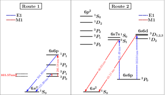
Figure 3: Schematic energy level diagram for $6s^{2}\;{}^{1}S_{0}\rightarrow 6s6p\;^{3}P^{o}_{0}$ clock transition in Pb²⁺ via a two photon E1+M1 transition.

IV Results and discussions

IV.1 Single-particle basis and convergence of properties

An accurate description of single-electron wave functions and corresponding energies are crucial to obtain the reliable results using FSRCC theory. In the present work, we have used the Gaussian-type orbitals (GTOs) Mohanty et al. (1991) as the single-electron basis for FSRCC calculations. The GTOs are used as the finite basis sets in which the single-electron wave functions are expressed as a linear combination of the Gaussian-type functions (GTFs). More precisely, the GTFs of the large component of the wavefunction are expressed as

$$g^{L}_{\kappa p}(r)=C^{L}_{\kappa i}r^{n_{\kappa}}e^{-\alpha_{p}r^{2}},$$ (9)

where $p=0$, $1$, $2$, $\ldots$, $N$ is the GTO index and $N$ is the total number of GTFs. The exponent $\alpha_{p}$ is further expressed as $\alpha_{0}\beta^{p-1}$, where $\alpha_{0}$ and $\beta$ are the two independent parameters. The parameters $\alpha_{0}$ and $\beta$ are optimized separately for each orbital symmetry so that the single-electron wavefunctions and energies match well with the numerical values obtained from the GRASP2K Jönsson et al. (2013). The small components of wavefunctions are derived from the large components using the kinetic balance condition Stanton and Havriliak (1984).

Table 1: The single-particle and SCF energies (in a.u.) from GTO compared with GRASP2K and B-Spline results. The optimized $\alpha_{0}$ and $\beta$ parameter for the even tempered basis used in our calculations are also provided.

Orbitals	GTO	GRASP2K	B-Spline
$1s_{1/2}$	-3257.41150	-3257.40298	-3257.41571
$2s_{1/2}$	-589.39795	-589.39605	-589.39835
$2p_{1/2}$	-565.00395	-565.00364	-565.00295
$2p_{3/2}$	-484.41530	-484.41512	-484.41548
$3s_{1/2}$	-145.26466	-145.26400	-145.26472
$3p_{1/2}$	-134.31668	-134.31639	-134.31638
$3p_{3/2}$	-116.10663	-116.10639	-116.10665
$3d_{3/2}$	-98.32473	-98.32446	-98.32473
$3d_{5/2}$	-94.48445	-94.48420	-94.48445
$4s_{1/2}$	-35.49304	-35.49280	-35.49305
$4p_{1/2}$	-30.72284	-30.72269	-30.72276
$4p_{3/2}$	-26.20738	-26.20725	-26.20737
$4d_{3/2}$	-18.43141	-18.43130	-18.43141
$4d_{5/2}$	-17.57859	-17.57861	-17.57859
$4f_{5/2}$	-7.44501	-7.44494	-7.44502
$4f_{7/2}$	-7.25330	-7.25331	-7.25331
$5s_{1/2}$	-7.63856	-7.63855	-7.63857
$5p_{1/2}$	-5.94459	-5.94458	-5.94458
$5p_{3/2}$	-5.09665	-5.09664	-5.09666
$5d_{3/2}$	-2.62373	-2.62373	-2.62373
$5d_{5/2}$	-2.51852	-2.51852	-2.51852
$E_{\rm SCF}$	-20910.40152	-20910.37469	-20910.40151
	$\alpha_{0}$	$\beta$	GTOs
$s$	0.00450	1.805	40
$p$	0.00478	1.792	38
$d$	0.00605	1.855	34
$f$	0.00355	1.845	28

In Table 1, we have provided the optimized values of $\alpha_{0}$ and $\beta$ parameters for Pb²⁺ and have compared the values of single-electron and self-consistent field (SCF) energies with GRASP2K Jönsson et al. (2013) and B-spline Zatsarinny and Fischer (2016) results. It is to be mentioned that, the single-electron basis used in the properties calculations also incorporates the effects of Breit interaction, vacuum polarization and the self-energy corrections. As evident from the table, the single-particle and SCF energies are in excellent agreement with GRASP2K and B-spline results. The largest difference at the level of SCF and single-particle energies are 0.0001% and 0.0003%, respectively.

Since GTOs are a mathematically incomplete basis, convergence of the properties results with basis size must be checked to get reliable results using FSRCC. To show the convergence of properties results, in Table 8 of Appendix, we have listed the values of electric dipole polarizability and E1 and M1 transition reduced matrix elements for increasing basis size. To achieve a converged basis, we start with a moderate basis size and add orbitals systematically in each symmetry until the change in the properties is less than or equal to $10^{-3}$ in respective units. For example, as evident from the table, the change in E1 amplitude of $\langle^{1}S_{0}||D||^{1}P^{o}_{1}\rangle$ transition is of the order of $10^{-3}$ a.u. when basis is augmented from 158 ($24s21p18d13f8g7h$) to 169 ($25s22p19d14f9g8h$) orbitals. So, to minimize the compute time, we consider the basis set with 158 orbitals as optimal, and use it for further FSRCC calculations where the corrections from the Breit interaction, vacuum polarization and the self-energy are incorporated.

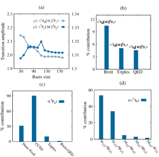
Figure 4: Convergence of transition amplitudes with basis size, panel (a). Dominant percentage contributions from Breit, perturbative triples and QED corrections to the reduced matrix elements, panel (b), and the lifetime of the clock state, panel (c). Dominant contributions from core orbitals to the dipole polarizability, panel (d).

IV.2 Excitation Energy

The eigen energies obtained from the solution of many-electron Schrodinger equation (1) using FSRCC are used to calculate the excitation energies. The excitation energy of a general state $nln^{{}^{\prime}}l^{{}^{\prime}}{\;{}^{(2S+1)}}L_{J}$ is defined as

$$\Delta E_{nln^{{}^{\prime}}l^{{}^{\prime}}{\;{}^{(2S+1)}}L_{J}}=E_{nln^{{}^{\prime}}l^{{}^{\prime}}{\;{}^{(2S+1)}}L_{J}}-E_{ns^{2}{\;{}^{1}}S_{0}},$$ (10)

where $E_{ns^{2}{\;{}^{1}}S_{0}}$ and $E_{nln^{{}^{\prime}}l^{{}^{\prime}}{\;{}^{(2S+1)}}L_{J}}$ are the exact energies of the ground and excited states, respectively. In Table 2, we have provided the excitation energies from our calculations along with other theory and experimental data for comparison. To account for valence-valence correlations more accurately, we have also included $6p^{2}$, $6s6d$ and $6s7s$ high energy configurations in the model space. For a quantitative assessment of electron correlations, we have listed the contributions from Breit and QED corrections separately.

Table 2: The ground state energy of ${}^{1}S_{0}$ (cm^-1) and excitation energies of some low lying excited states of Pb²⁺. For quantitative analysis of electron correlations, contributions from Breit and QED corrections are given separately.

States	DC-CCSD	Breit	Self-energy	Vac-pol	Total	Other cal.	NISTNIS (2013)	% Error
$6s^{2}$ ${}^{1}S_{0}$	599355.44	12.00	-0.67	188.97	599556	600984Safronova et al. (2012)	598942	0.1
$6s6p$ ${}^{3}P^{o}_{0}$	59624.80	121.57	-0.58	81.41	59827	61283Safronova et al. (2012), 60653Curtis et al. (2001)	60397	0.94
$6s6p$ ${}^{3}P^{o}_{1}$	64146.99	116.92	-0.53	82.84	64346	65089Safronova et al. (2012), 65683Migdalek and Baylis (1985)	64391	0.06
						60387Migdalek and Bojara (1988),58905Chou and Huang (1992)
						64609Curtis et al. (2001)
$6s6p$ ${}^{3}P^{o}_{2}$	79478.69	83.67	-0.33	90.27	79652	80029Safronova et al. (2012), 79024Curtis et al. (2001)	78985	-0.8
$6s6p$ ${}^{1}P^{o}_{1}$	95045.89	83.07	-0.63	84.30	95213	95847Safronova et al. (2012), 97970Migdalek and Baylis (1985)	95340	0.13
						91983Migdalek and Bojara (1988), 95537Chou and Huang (1992)
						95535Curtis et al. (2001)
$6p^{2}$ ${}^{3}P_{0}$	142922.33	236.01	-1.41	169.97	143327	143571Safronova et al. (2012)	142551	-0.54
$6s7s$ ${}^{3}S_{1}$	149898.62	4.90	-0.32	64.10	149967	151183Safronova et al. (2012)	150084	0.07
$6s6d$ ${}^{1}D_{2}$	152651.06	108.27	-0.70	135.00	152894	153614Safronova et al. (2012)	151885	-0.6
$6s7s$ ${}^{1}S_{0}$	153901.92	3.47	-0.28	62.88	153968	155054Safronova et al. (2012)	153783	-0.12
$6p^{2}$ ${}^{3}P_{1}$	155401.22	189.27	-1.16	170.87	155760	156610Safronova et al. (2012)	155431	-0.2
$6s6d$ ${}^{3}D_{1}$	157523.12	17.37	-0.55	92.43	157632	158439Safronova et al. (2012)	157444	-0.1
$6s6d$ ${}^{3}D_{2}$	157902.47	5.93	-0.48	87.81	157996	159134Safronova et al. (2012)	157925	-0.04
$6s6d$ ${}^{3}D_{3}$	159147.60	0.04	-0.38	86.03	159233	160530Safronova et al. (2012)	158957	-0.17
$6p^{2}$ ${}^{3}P_{2}$	164987.49	117.07	-0.99	143.34	165247	165898Safronova et al. (2012)	164818	-0.26
$6p^{2}$ ${}^{1}D_{2}$	179412.09	139.08	-1.17	166.70	179717	179646Safronova et al. (2012)	178432	-0.7
$6p^{2}$ ${}^{1}S_{0}$	189714.06	161.46	-1.17	179.67	190054	190061Safronova et al. (2012)	188615	-0.7

^a Ref. Safronova et al. (2012) - CI + all-order , ^b Ref. Curtis et al. (2001) - MCDHF, ^c Ref. Migdalek and Baylis (1985) - CIRHF + CP, ^d Ref. Migdalek and Bojara (1988) - CIRHF + CP, ^e Ref. Chou and Huang (1992) - MCRRPA

As evident from the table, our computed energies are in excellent agreement with the experimental values. The largest relative error in our calculation is $\approx$ 0.9%, in the case of ${{}^{3}}P^{o}_{0}$ state. However, for other ASFs, specially for those which contribute to the lifetime of the clock state, the errors are much smaller. The ASFs ${{}^{3}}P^{o}_{1}$, ${{}^{1}}P^{o}_{1}$, ${{}^{3}}S_{1}$ and ${{}^{3}}D_{1}$, which couple either via E1 or M1 operator in clock transition, have the relative errors of 0.06%, 0.13%, 0.07% and -0.10%, respectively. This is crucial, as these energies contribute to the lifetime of the clock state. Among all the previous theory results listed in the table, Ref. Safronova et al. (2012) is close to ours in terms of the many-body methods used, however, with an important difference. Ref. Safronova et al. (2012) uses a linearized CCSD method, whereas the present work employs a nonlinear CCSD, which accounts for electron correlation effects more accurately in the calculation. The relative errors in the reported excitation energies for ${{}^{3}}P^{o}_{1}$, ${{}^{1}}P^{o}_{1}$, ${{}^{3}}S_{1}$ and ${{}^{3}}D_{1}$ states in Ref. Safronova et al. (2012) are 1.08%, 0.53%, 0.73% and 0.63%, respectively. Remaining results are mostly based on the multi-configuration Hartree-Fock and its variations and, in general, not very consistent in terms of treating electron correlations.

Examining the contributions from high energy configurations, we observed an improvement in the excitation energies of ${{}^{3}}P^{o}_{1}$ and ${{}^{1}}P^{o}_{1}$ states due to accounting of valence-valence correlation more accurately. We find that the relative error has reduced from 0.7% (0.6%) to 0.4% (0.3%) for ${{}^{3}}P^{o}_{1}$(${{}^{1}}P^{o}_{1}$) state. Among the contributions from Breit, vacuum polarization and self-energy corrections, the former two are observed to contribute more. The largest cumulative contribution of about $0.3$% from Breit and vacuum polarization is observed in the case of ${}^{3}P^{o}_{0}$. Self-energy contributions are of opposite phase and negligibly small.

IV.3 E1 Reduced Matrix Elements

In Table 3, we have provided the values of E1 reduced matrix elements from our calculations for all dominant transitions which contribute to the lifetime of the clock state. Since there are more data on oscillator strengths from literature, we converted E1 reduced matrix elements to oscillator strength and tabulated in the table for comparison with experiments and other theory calculations. The contributions from Breit+QED and triples are provided separately in the table. As evident from the table, as to be expected, DC-CCSD gives the dominant contribution to all the matrix elements. The contributions from Breit, QED and perturbative triples are small but important to get accurate results of the properties. A quantitative analysis on these is provided later in the section.

Table 3: The E1 and M1 reduced matrix elements (a.u.) and oscillator strengths for some allowed transitions in Pb²⁺. For comparison, data from experiments and other theory calculations are also provided.

States	DC-CCSD	Breit + QED	P-triples	Total	Other cal.	Expt.
E1 Reduced Matrix Elements
$\langle^{1}S_{0}||D||^{3}P^{o}_{1}\rangle$	0.5359	-0.0007	-0.0130	0.5222	0.706Beloy (2021), 0.644Safronova et al. (2012)
$\langle^{1}S_{0}||D||^{1}P^{o}_{1}\rangle$	1.9854	-0.0006	-0.0131	1.9717	2.350Beloy (2021), 2.384Safronova et al. (2012)
$\langle^{3}S_{1}||D||^{3}P^{o}_{0}\rangle$	0.5363	-0.0005	-0.0232	0.5126	0.963Safronova et al. (2012)
$\langle^{3}D_{1}||D||^{3}P^{o}_{0}\rangle$	-1.4985	0.0155	-0.0676	-1.5506	-1.516Safronova et al. (2012)
Oscillator Strengths
$\langle^{1}S_{0}||D||^{3}P^{o}_{1}\rangle$	5.5716[-2]	0.0025[-2]	-0.2327[-2]	5.3414[-2]	8.11[-2]Safronova et al. (2012), 7.40[-2]Alonso-Medina et al. (2009), 5.44[-2]Migdalek and Baylis (1985),	(7.3 $\pm$ 0.5)[-2]Pinnington et al. (1988), Ansbacher et al. (1988)
					7.55[-2]Glowacki and J.Migdalek (2003), 6.15[-2]Chou and Huang (1992), 6.15[-2]Chou and Huang (1997)
					5.52[-2]Migdalek and Bojara (1988)
$\langle^{1}S_{0}||D||^{1}P^{o}_{1}\rangle$	1.1317	0.0013	-0.0092	1.1238	1.65Safronova et al. (2012), 1.24Alonso-Medina et al. (2009), 1.64Migdalek and Baylis (1985), 1.51Glowacki and J.Migdalek (2003),	(1.01 $\pm$ 0.20)Andersen et al. (1972)
					2.45Chou and Huang (1992), 1.42Chou and Huang (1997), 1.43Migdalek and Bojara (1988)
$\langle^{3}S_{1}||D||^{3}P^{o}_{0}\rangle$	0.0788	0	-0.0069	0.0719	0.229Alonso-Medina et al. (2009)
$\langle^{3}D_{1}||D||^{3}P^{o}_{0}\rangle$	0.6664	-0.0130	0.0589	0.7123	0.93Alonso-Medina et al. (2009)
M1 Reduced Matrix Elements
$\langle^{3}P^{o}_{1}||M1||^{3}P^{o}_{0}\rangle$	-1.3117	-0.0002	0.0001	-1.3118	-0.674Beloy (2021)
$\langle^{1}P^{o}_{1}||M1||^{3}P^{o}_{0}\rangle$	0.4959	-0.0003	0.0001	0.4957	0.205Beloy (2021)
$\langle^{1}S_{0}||M1||^{3}S_{1}\rangle$	0.0046	-0.0004	-0.0002	0.0040
$\langle^{1}S_{0}||M1||^{3}D_{1}\rangle$	-0.0116	-0.0019	0.0006	-0.0129

^a Ref. Beloy (2021) - CI + MBPT , ^b Ref. Alonso-Medina et al. (2009) - IC + RHF +CP, ^c Ref. Glowacki and J.Migdalek (2003) - CIDF - MP, ^d Ref. Chou and Huang (1997) - MCRRPA, ^e Ref. Safronova et al. (2012) - CI + all-order, ^f Ref. Colón and Alonso-Medina (2000) - IC + RHF, ^g Ref. Migdalek and Bojara (1988) - CIRHF + CP, ^h Ref. Chou and Huang (1992) - MCRRPA, ⁱ Ref. Migdalek and Baylis (1985) - CIRHF + CP,

From previous theory calculations, to the best of our knowledge, we found two works, Refs. Beloy (2021)-CI+MBPT and Safronova et al. (2012)-CI+all-order, for comparison of E1 reduced matrix elements. The values of our E1 reduced matrix elements are slightly on the smaller sides of Refs. Beloy (2021) and Safronova et al. (2012) for all the listed transitions. The reason for this could be attributed to the different treatment of electron correlations in these methods. In Ref. Beloy (2021), MBPT is used to treat core-core and core-valence correlations, whereas valence-valence correlation is treated in the framework of configuration interaction (CI). In Ref. Safronova et al. (2012), however, the core-core and core-valence correlations are accounted using a linearized CCSD method. The present work, however, employs a nonlinear CCSD theory to account for the core-core and core-valence correlations and, therefore, is more accurate. The valence-valence correlation is however treated in the same way as in Refs. Beloy (2021); Safronova et al. (2012). The other two important inclusions in the present work are, the use of high energy configurations ($6p^{2}$, $6s7s$ and $6s6d$) in the model space and the corrections from the Breit, QED and perturbative triples.

For oscillator strengths, from other theory calculations, there are several data in the literature for $\langle^{1}S_{0}||D||^{3}P^{o}_{1}\rangle$ and $\langle^{1}S_{0}||D||^{1}P^{o}_{1}\rangle$ transitions for comparison. As evident from the table, there is, however, a large variation in the reported values. For example, for $\langle^{1}S_{0}||D||^{3}P^{o}_{1}\rangle$ transition, the smallest value $5.44\times 10^{-2}$ from Ref. Migdalek and Baylis (1985) differs by $\approx$ 33% with the largest value $8.11\times 10^{-2}$ reported in the Ref Safronova et al. (2012). The similar trend is also observed for $\langle^{1}S_{0}||D||^{1}P^{o}_{1}\rangle$ transition. The smallest value, 1.24 Alonso-Medina et al. (2009), is almost half the largest value, 2.45 Chou and Huang (1992). The reason for this large variation could be attributed to the different many-body methods employed in these calculations. It is to be noted that, none of the previous calculations use FSRCC theory, like the case of the present work. Except Ref. Safronova et al. (2012), which uses CI + all-order, the other calculations are mostly based on the MCDF and its variations. The large difference among these results clearly indicates the inherent inconsistencies with MCDF methods in terms of incorporating electron correlation effects in many-body calculation. For $\langle^{1}S_{0}||D||^{3}P^{o}_{1}\rangle$ transition, our result, $5.34\times 10^{-2}$, lies in the range of the previous values. Whereas, for transition $\langle^{1}S_{0}||D||^{1}P^{o}_{1}\rangle$, our value, 1.12, is smallest among all results listed in the table.

From experiments, to the best of our knowledge, there is one result each for oscillator strength for $\langle^{1}S_{0}||D||^{3}P^{o}_{1}\rangle$ Pinnington et al. (1988) and $\langle^{1}S_{0}||D||^{1}P^{o}_{1}\rangle$ Andersen et al. (1972) transitions. Both of these experiments use the beam-foil technique to study atomic spectra. For $\langle^{1}S_{0}||D||^{3}P^{o}_{1}\rangle$ transition, our calculated result, $5.34\times 10^{-2}$, is of the same order of magnitude as the experimental value, $(7.3\pm 0.5)\times 10^{-2}$, but smaller by about 27%. Among the previous theory calculations, the MCDF calculations Refs. Alonso-Medina et al. (2009) and Glowacki and J.Migdalek (2003) are more closer to the experiment. For $\langle^{1}S_{0}||D||^{1}P^{o}_{1}\rangle$ transition, however, among all the theory results listed in table, our result, 1.12, shows the best match to the experimental result, $1.01\pm 0.20$ Andersen et al. (1972).

Table 4: Termwise contributions to E1 and M1 reduced matrix elements (a.u.) from different terms in FSRCC theory. The operator $\hat{O}$ is either electric or magnetic dipole operator.

Terms + h. c.	$\langle^{1}S_{0}||D||^{1}P^{o}_{1}\rangle$	$\langle^{3}P^{o}_{1}||M1||^{3}P^{o}_{0}\rangle$
DF	$2.1553$	$1.3586$
1v diagrams	$-0.4040$	$0.0122$
$\hat{O}R_{2}$	$0.1049$	$-0.0199$
${R_{2}}\hat{O}{R_{2}}$	$0.0711$	$-0.0423$
${S_{1}}\hat{O}{R_{2}}+{S_{2}}\hat{O}{R_{2}}+{S_{1}^{2}}\hat{O}{R_{2}}$	$0.0074$	$0.0081$
$\hat{O}S_{2}$	$0.0063$	$-0.0003$
${S_{2}}\hat{O}{S_{2}}+{S_{2}}\hat{O}{S_{1}}+{S_{2}}\hat{O}{S_{1}^{2}}$	$0.0310$	$-0.0046$
${T_{1}}\hat{O}{R_{2}}$	$-0.0001$	$0$
${S_{2}}\hat{O}{T_{2}}+{S_{2}}\hat{O}{T_{1}}$	$0.0007$	$0$
${T_{2}}\hat{O}{T_{2}}+{T_{1}}\hat{O}{T_{2}}$	$0.0003$	$0$
Total	$1.9729$	$1.3118$

IV.4 M1 Reduced Matrix Elements

Next, we present and analyze the M1 reduced matrix elements for transitions which contribute dominantly to the lifetime of the clock state. These are given in the Table 3. As to be expected, like the case of E1 matrix elements, the most dominant contribution is from DC-CCSD for all the transitions. The cumulative contribution from Breit, QED and perturbative triples are small but important to get a reliable transition properties results.

Unlike the E1 matrix elements, for M1 there are not much data available from literature for comparison. To the best of our knowledge, there is only one theory calculation using CI+MBPT Beloy (2021), which reports the values of M1 reduced matrix elements for $\langle^{3}P^{o}_{1}||M1||^{3}P^{o}_{0}\rangle$ and $\langle^{1}P^{o}_{1}||M1||^{3}P^{o}_{0}\rangle$ transitions. Interestingly, unlike the E1 reduced matrix elements where the two works are comparable, our results for M1 reduced matrix elements differ by a factor of two or more to Ref. Beloy (2021). This is expected to lead to a large difference between the lifetimes calculated using the two data. Since there are no other theory or experimental results to compare for Pb²⁺, to cross check and validate our M1 implementation within FSRCC, we calculated and compared results for other atomic systems. Ref. Dzuba et al. (2018), using a combined method of configuration interaction (CI) and perturbation theory (PT), reports the value of M1 transition rate for $\langle^{3}P^{o}_{2}||M1||^{3}P^{o}_{1}\rangle$ transition in neutral Yb as $6.7\times 10^{-2}$ s^-1. And our computed value is $5.3\times 10^{-2}$ s^-1. It should be noted that the difference, $\approx$ 21%, is much smaller than that of our M1 reduced matrix elements with Ref. Beloy (2021) in the case of Pb²⁺. Reason for this could be attributed to the more accurate treatment of electron correlations in FSRCC theory. In an another work, Ref. Derevianko (2001) using CI+RPA has computed and reported the value of transition rate for $\langle^{3}P^{o}_{2}||M1||^{3}P^{o}_{1}\rangle$ transition in neutral Sr. The reported value, $8.26\times 10^{-4}$, compares well with our computed value, $8.88\times 10^{-4}$, except with a small difference of about 7% which could again be due to a better accounting of electron correlations in FSRCC. In yet another seminal work, Ref. Safronova et al. (1999a) carried out a second-order MBPT calculation of M1 reduced matrix elements for $\langle^{3}P^{o}_{0}||M1||^{3}P^{o}_{1}\rangle$ and $\langle^{3}P^{o}_{0}||M1||^{1}P^{o}_{1}\rangle$ transitions in Fe²²⁺. The reported values, 1.40 and 0.22, respectively are in good agreement with our computed values, 1.37 and 0.28.

IV.5 Lifetime of Clock State

Next, using the E1 and M1 reduced matrix elements from Table 3 and excitation energies from Table 2 in Eq. (7), we calculated the E1M1 decay rate ($\Gamma$) for $6s^{2}{\;{}^{1}}S_{0}\rightarrow 6s6p{\;{}^{3}}P^{o}_{0}$ clock transition, inverse of which gives the lifetime ($\tau$) of the clock state. The $\Gamma$ and $\tau$ obtained from our calculations are given in the Table 5. To assess the effect of valence-valence correlation, we have separately given the contributions from $6s6p$, $6s7s$ and $6s6d$ configurations. Our computed lifetime, $10.45\times 10^{6}$ s, is about 16% larger than the only calculation Ref. Beloy (2021). The reason for this could be attributed to the more accurate treatment of electron correlations in our calculations. It should be noted that, our calculations also incorporate the contributions from E1 and M1 matrix elements from higher energy ASFs, $6s6d{\;{}^{3}}D_{1}$ and $6s7s{\;{}^{3}}S_{1}$. This has a significant cumulative contribution of $\approx$ 2.8% to the total lifetime. The other key difference from Ref. Beloy (2021) is, the inclusion of the corrections from Breit, QED and perturbative triples in our calculations. It is to be noted that the contribution from perturbative triples is significant, it contributes approximately about 10% to the lifetime. This is consistent with our previous work on Al⁺ clock where we observed a large contribution of about 6% to the lifetime of the clock state Kumar et al. (2021a). Contributions from Breit and QED corrections are small but important to get accurate value of lifetime. The combined contribution from Breit+QED is observed to be $\approx$ 0.5%. As discernible from the Fig. 4(c), DF alone contributes about 30% of the total value. The most significant contribution comes from the electron correlations arising from the residual Coulomb interaction through FSRCC within CCSD framework. The cumulative contribution from DF and CCSD is about 90% of the total lifetime.

Table 5: E1M1 decay rate and lifetime of the clock state ${}^{3}P^{o}_{0}$. Tabulated results also incorporate the contributions from the Breit, QED and perturbative triples corrections.

Configurations	$\Gamma$ (sec-1)	$\tau$ (sec)
6s2 + 6s6p	$9.931\times 10^{-8}$	$10.195\times 10^{6}$
6s2 + 6s6p + 6s7s	$9.902\times 10^{-8}$	$10.224\times 10^{6}$
6s2 + 6s6p + 6s7s + 6s6d	$9.661\times 10^{-8}$	$10.448\times 10^{6}$
Recommended	$9.661\times 10^{-8}$	$(10.45\pm 0.50)\times 10^{6}$
Others		$9\times 10^{6}$Beloy (2021)

IV.6 Dipole Polarizability

The electric dipole polarizability, $\alpha$, is a measure of the interaction between electrons’ and nuclear moments, and provides an important probe to several fundamental properties Khriplovich (1991); Griffith et al. (2009); Karshenboim and Peik (2010). In the context of the present work, $\alpha$ is needed for calculating the BBR shift in the clock transition frequency. In Table 6, we present our result on $\alpha$ for the ground state of Pb²⁺ and compare with data in the literature. To calculate this, we have used the PRCC theory developed and presented in our previous works Kumar et al. (2020, 2021b). Table 6 also shows the contributions from various correlation terms embedded in the PRCC theory. The term estimated identifies the contribution from the orbitals from $i$, $j$ and $k$-symmetries. As to be expected, the dominant contribution is from the DF term. It contributes about 116% of the total value. The PRCC value is $\approx$ 13% smaller than the DF value. The reason for this is the cancellation due to opposite contributions from electron correlation.

Table 6: The value of $\alpha$ (a.u.) for ground state, $6s^{2}\;{}^{1}S_{0}$, of Pb²⁺ from PRCC calculation. The available data from experiment and other theory calculations are also provided for comparison.

State	Present work
	Method	$\alpha$
$6s^{2}\;{}^{1}S_{0}$	DF	$16.246$
	PRCC	$14.173$
	PRCC(T)	$14.166$
	PRCC(T)+Breit	$14.173$
	PRCC(T)+Breit+QED	$14.064$
	Estimated	$14.016$
	Recommended	$14.02\pm 0.21$
	Other cal.	$13.3\pm 0.4^{\rm a}$
	Expt.	$13.62\pm 0.08^{\rm b}$

aRef.Safronova et al. (2012)-CI + all-order, bRef.Hanni et al. (2010)-Expt.

Table 7: Termwise contributions to $\alpha$ (a.u.) from different terms in PRCC theory.

Terms + h. c.	$\alpha$
${{\mathbf{T}}_{1}^{(1)\dagger}{\mathbf{D}}}$	$16.6849$
${\mathbf{T}_{1}}{{}^{(1)\dagger}}{\mathbf{D}}T_{2}^{(0)}$	$-1.0835$
${\mathbf{T}_{1}}{{}^{(1)\dagger}}{\mathbf{D}}T_{1}^{(0)}$	$-0.2746$
${\mathbf{T}_{2}}{{}^{(1)\dagger}}{\mathbf{D}}T_{1}^{(0)}$	$-0.0052$
${\mathbf{T}_{2}}{{}^{(1)\dagger}}{\mathbf{D}}T_{2}^{(0)}$	$0.4145$
Normalization	$-1.5633$
Total	$14.1733$

Comparing our result with data in literature, to the best of our knowledge, we found one result each from the experiment and other theory calculation. Our recommended value, 14.02, is in good agreement with the experimental value, 13.62$\pm$0.08, reported in Ref. Hanni et al. (2010). The difference from the experiment is about 3%. From theory calculation, Safronova and collaborators Safronova et al. (2012) have reported the value of 13.3 using the CI+all-order method. Our recommended result is about 6% larger than Ref. Safronova et al. (2012). As mentioned earlier, reason for this difference could be attributed to the more accurate treatment of electron correlations in the present calculation. The other key merit in the present calculation is that, it does not employ the sum-over-state Safronova et al. (1999b); Derevianko et al. (1999) approach to incorporate the effects of perturbation. The summation over all the possible intermediate states is accounted through the perturbed cluster operators Kumar et al. (2020, 2021a). In addition, the present work also incorporates the effects of Breit, QED and perturbative triples corrections in the calculation of $\alpha$.

IV.7 Electron Correlations in FSRCC and PRCC Theories and Corrections from Breit, QED and Perturbative Triples

Next, we analyze and present the trend of contributions from various correlation terms in FSRCC and PRCC theories, and from the Breit and QED corrections. As mentioned earlier, FSRCC method is used to calculate the lifetime of the metastable clock state, whereas PRCC theory is employed to calculate $\alpha$ for the ground state of Pb²⁺.

In Table 4, we have provided the term-wise contributions from FSRCC for one each from E1 and M1 matrix elements. As expected, the leading order (LO) contribution to both the matrix elements is from the Dirac-Fock (DF). It contributes $\approx$ 109 and 104% of the total value for $\langle^{1}S_{0}||D||^{1}P^{o}_{1}\rangle$ and $\langle^{3}P^{o}_{1}||M1||^{3}P^{o}_{0}\rangle$, respectively. As the next leading order (NLO) contribution, the two matrix elements show a different trend. For $\langle^{1}S_{0}||D||^{1}P^{o}_{1}\rangle$, the NLO contribution of opposite phase of $\approx$ -20% is observed from the one-valence sector. Whereas, for $\langle^{3}P^{o}_{1}||M1||^{3}P^{o}_{0}\rangle$, the NLO contribution is observed from the two-valence sector, where an opposite contribution of $\approx$ -3% is observed from the ${R_{2}}\hat{O}{R_{2}}$ term. As the next dominant contribution, the term $\hat{O}{R_{2}}+{\rm h.c.}$ contributes $\approx$ 5 and 1.5%, respectively, to $\langle^{1}S_{0}||D||^{1}P^{o}_{1}\rangle$ and $\langle^{3}P^{o}_{1}||M1||^{3}P^{o}_{0}\rangle$ matrix elements.

For the contributions from the Breit and QED corrections to matrix elements, the largest combined contribution is observed to be $\approx$ 1.0%, in the case of $\langle^{3}D_{1}||D||^{3}P^{o}_{0}\rangle$ transition. Whereas, the largest contribution from the perturbative triples is observed to be $\approx$ 4.4%, in the case of $\langle^{3}D_{1}||D||^{3}P^{o}_{0}\rangle$. Combining these two, the largest cumulative contribution from Breit+QED+perturbative triples is observed to $\approx$ 5.5%. Considering the high accuracies associated with atomic clocks, this is a significant contribution and important to be included in the calculations to get accurate clock properties results.

To understand the nature of electron correlations embedded in $\alpha$, in Table 7 we have listed the termwise contributions from PRCC theory. As evident from the table, the LO term, ${{\mathbf{T}}_{1}^{(1)\dagger}{\mathbf{D}}}$ + h. c., contributes $\approx$ 118% of the total value. This is expected, as it includes the DF and dominant contribution from core-polarization. For a better illustration, in Fig. 4(d), we have shown the five dominant contributions from core orbitals. As discernible from the figure, about 87% of the LO contribution comes from $6s$ valence-electrons through the dipolar mixing with $6p$ states. This is expected due to the larger radial extent of $6s$ orbital. In remaining LO contribution, a contribution of about 8.5% is observed from the $5d$ core-electrons, through the dipolar mixing with $6p$ and $4f$-electrons. The NLO term is ${\mathbf{T}_{1}}{{}^{(1)\dagger}}{\mathbf{D}}T_{2}^{(0)}$, contributes $\approx$ 8%. It is to be noted that, it accounts for the dominant pair-correlation effects through the $T_{2}^{(0)}$ operator. The next dominant contribution of about 3%, which also include some part of pair-correlation, is from the term ${\mathbf{T}_{2}}{{}^{(1)\dagger}}{\mathbf{D}}T_{2}^{(0)}$.

The perturbative triples and Breit each contributes about 0.04% to $\alpha$. The contribution from QED is, however, significant, about 0.7%. So, the cumulative contribution from Breit+QED+perturbative triples is $\approx$ 0.8%. The contribution from the higher symmetry orbitals is estimated to be about 0.34% of the total value.

V Theoretical Uncertainty

The uncertainty in the calculated lifetime of clock state will depend on the uncertainties in the E1 and M1 matrix elements and the energy denominators, as they contribute in Eq. (7). As the experimental results are not available for all the E1 and M1 reduced matrix elements, we have identified four different sources which can contribute to the uncertainty in E1 and M1 matrix elements. The first source of uncertainty is due to the truncation of the basis set in our calculation. As discussed in the basis convergence section, our calculated values of E1 and M1 reduced matrix elements converge to the order of $10^{-3}$ or smaller with basis. Since this is a very small change, we can neglect this uncertainty. The second source of uncertainty arises due to the truncation of the dressed Hamiltonian $\tilde{H}^{\rm e}_{\rm hfs}$ to the second order in $T^{(0)}$ in the properties calculation. In our earlier work Mani and Angom (2010), using an iterative scheme, we found that the terms with third and higher orders in $T^{(0)}$ contribute less than 0.1%. So, we consider 0.1% as an upper bound for this source. The third source is due to the partial inclusion of triple excitations in the properties calculation. Since perturbative triples account for the leading order terms of triple excitation, the contribution from remaining terms will be small. Based on the analysis from our previous works Kumar et al. (2020); Chattopadhyay et al. (2015) we estimate the upper bound from this source as 0.72%. The fourth source of uncertainty could be associated with the frequency-dependent Breit interaction which is not included in the present calculations. However, in our previous work Chattopadhyay et al. (2014), using a series of computations using GRASP2K we estimated an upper bound on this uncertainty as $0.13$% in Ra. So, for the present work, we take $0.13$% as an upper bound from this source. There could be other sources of theoretical uncertainty, such as the higher order coupled perturbation of vacuum polarization and self-energy terms, quadruply excited cluster operators, etc. However, in general, these all have much lower contributions to the properties and their cumulative theoretical uncertainty could be below 0.1%. Uncertainty in the energy denominator is estimated using the relative errors in the energy difference of ${}^{3}P^{o}_{1}$, ${}^{1}P^{o}_{1}$, ${}^{3}S_{1}$ and ${}^{3}D_{1}$ intermediate states with respect to ${}^{3}P^{o}_{0}$. Among all the intermediate states, ${}^{1}P^{o}_{1}$ and ${}^{3}D_{1}$ states contribute dominantly, through routes 1 and 2, respectively, to the lifetime. The relative errors in the energy difference of these states with ${}^{3}P^{o}_{0}$ are 1.27% and 0.78%, respectively. Since they correspond to the dominant contributions, we have taken them as the uncertainty in the energy denominator. By combining the upper bounds of all the uncertainties, the theoretical uncertainty associated with the lifetime of the clock state is $\approx$ 4.8%. It should, however, be noted that the uncertainty in the value of $\alpha$ is much smaller, about 1.5% Kumar et al. (2022)

VI Conclusions

We have employed an all-particle multireference Fock-space relativistic coupled-cluster theory to examine the clock transition properties in Pb²⁺. We have computed the excitation energies for several low lying states and E1 and M1 transition amplitudes for all the allowed transitions in the considered model space. These were then used to calculate the lifetime of the clock state. Moreover, using PRCC theory, we also calculated the electric dipole polarizability for the ground state of Pb²⁺. In all these calculations, to obtain accurate properties results, we incorporated the corrections from the relativistic and QED effects. The dominant contribution from triple excitations was incorporated though perturbative triples and a fairly large basis sets were used to achieve the convergence of the properties.

Our computed excitation energies are in excellent agreement with experimental values for all the states. Our calculated value of lifetime is about 16% larger than the previously reported CI+MBPT value in Ref. Beloy (2021). The reason for the higher lifetime in the present calculation could partially be attributed to the more accurate treatment of core-core and core-valence electron correlations in FSRCC theory. In addition, to account for the valence-valence correlation more accurately, we also incorporated the contributions from the higher energy configurations $6s6d$ and $6s7s$ in our calculation. Based on our analysis, we find that this contributes about 2.8% of the total lifetime. Also, from our study, we find that the contributions from the perturbative triples and Breit+QED corrections are crucial to get reliable lifetime of the clock state. They are observed to contribute $\approx$ 10% and 0.5%, respectively. Our recommended value of dipole polarizability is in good agreement with the available experimental value, with a small difference of about 3%. Based on our analysis on theoretical uncertainty, the upper bound on uncertainty for calculated lifetime is about 4.8%, whereas for polarizability it is about 1.5%.

Appendix A Convergence of $\alpha$ and E1 and M1 matrix elements

In Table 8, we provide the trend of the convergence of dipole polarizability and E1 and M1 matrix elements as a function of the basis size. As it is evident from the table, all the properties converge to the order of $10^{-3}$ or less in the respective units of the properties.

Table 8: Convergence trend of $\alpha$, and E1 and M1 matrix elements as a function of basis size.

Basis	$\alpha$	$\langle^{1}S_{0}||D||^{1}P^{o}_{1}\rangle$	$\langle^{3}P^{o}_{1}||M1||^{3}P^{o}_{0}\rangle$
$96:20s15p12d7f4g0h$	$15.919$	2.0512	1.3158
$103:19s16p13d8f3g2h$	$15.660$	2.0268	1.3153
$114:20s17p14d9f4g3h$	$14.979$	1.9966	1.3198
$125:21s18p15d10f5g4h$	$14.467$	1.9873	1.3134
$136:22s19p16d11f6g5h$	$14.274$	1.9888	1.3126
$147:23s20p17d12f7g6h$	$14.205$	1.9883	1.3121
$158:24s21p18d13f8g7h$	$14.175$	1.9875	1.3118
$169:25s22p19d14f9g8h$	$14.173$	1.9854	1.3117

References

- Ludlow et al. (2015) A. D. Ludlow, M. M. Boyd, J. Ye, E. Peik, and P. O. Schmidt, “Optical atomic clocks,” Rev. Mod. Phys. 87, 637–701 (2015).
- De and Sharma (2023) S. De and A. Sharma, “Indigenisation of the Quantum Clock: An Indispensable Tool for Modern Technologies,” Atoms 11, 71 (2023).
- Safronova (2019) M. S. Safronova, “The search for variation of fundamental constants with clocks,” Annalen der Physik 531, 1800364 (2019).
- Prestage et al. (1995) J. D. Prestage, R. L. Tjoelker, and L. Maleki, “Atomic clocks and variations of the fine structure constant,” Phys. Rev. Lett. 74, 3511–3514 (1995).
- Karshenboim and Peik (2010) S. G. Karshenboim and E Peik, Astrophysics, Clocks and Fundamental Constants, Lecture Notes in Physics (Springer, New York, 2010).
- Dzuba et al. (2018) V. A. Dzuba, V. V. Flambaum, and S. Schiller, “Testing physics beyond the standard model through additional clock transitions in neutral ytterbium,” Phys. Rev. A 98, 022501 (2018).
- Berengut et al. (2018) J. C. Berengut, D. Budker, C. Delaunay, V. V. Flambaum, C. Frugiuele, E. Fuchs, C. Grojean, Roni Harnik, R. Ozeri, G. Perez, and Y. Soreq, “Probing new long-range interactions by isotope shift spectroscopy,” Phys. Rev. Lett. 120, 091801 (2018).
- Grewal et al. (2013) M. S. Grewal, A. P. Andrews, and C. G. Bartone, Global Navigation Satellite Systems, Inertial Navigation, and Integration (John Wiley and Sons, New York, 2013).
- Major (2013) F.G. Major, The Quantum Beat: The Physical Principles of Atomic Clocks (Springer New York, 2013).
- Weiss and Saffman (2017) D. S. Weiss and M. Saffman, “Quantum computing with neutral atoms,” Physics Today 70, 44–50 (2017).
- Wineland et al. (2002) D. J. Wineland, J. C. Bergquist, J. J. Bollinger, R. E. Drullinger, and W. M. Itano, “Quantum computers and atomic clocks,” in Frequency Standards and Metrology (2002) pp. 361–368.
- Riehle et al. (2018) F. Riehle, P. Gill, F. Arias, and L. Robertsson, “The CIPM list of recommended frequency standard values: guidelines and procedures,” Metrologia 55, 188 (2018).
- Brewer et al. (2019) S. M. Brewer, J.-S. Chen, A. M. Hankin, E. R. Clements, C. W. Chou, D. J. Wineland, D. B. Hume, and D. R. Leibrandt, “ quantum-logic clock with a systematic uncertainty below ,” Phys. Rev. Lett. 123, 033201 (2019).
- Kállay et al. (2011) M. Kállay, H. S. Nataraj, B. K. Sahoo, B. P. Das, and L. Visscher, “Relativistic general-order coupled-cluster method for high-precision calculations: Application to the Al+ atomic clock,” Phys. Rev. A 83, 030503 (2011).
- Safronova et al. (2011) M. S. Safronova, M. G. Kozlov, and C. W. Clark, “Precision Calculation of Blackbody Radiation Shifts for Optical Frequency Metrology,” Phys. Rev. Lett. 107, 143006 (2011).
- Kumar et al. (2021a) R. Kumar, S. Chattopadhyay, D. Angom, and B. K. Mani, “Fock-space relativistic coupled-cluster calculation of a hyperfine-induced clock transition in Al+,” Phys. Rev. A 103, 022801 (2021a).
- Nicholson et al. (2015) T. Nicholson, S. Campbell, R. Hutson, E. Marti, B. Bloom, R. McNally, W. Zhang, M. Barrett, M. Safronova, G. Strouse, W. Tew, and J. Ye, “Systematic evaluation of an atomic clock at 2 x 10-18 total uncertainty,” Nature Communications 6, 6896 (2015).
- Bothwell et al. (2019) T. Bothwell, D. Kedar, E. Oelker, J. Robinson, S. Bromley, We. Tew, Ju. Ye, and C. Kennedy, “JILA Sr I optical lattice clock with uncertainty of 2.0×10⁻¹⁸,” Metrologia 56, 065004 (2019).
- Beloy (2021) K. Beloy, “Prospects of a Pb2+ ion clock,” Phys. Rev. Lett. 127, 013201 (2021).
- Pal et al. (2007) R. Pal, M. S. Safronova, W. R. Johnson, A. Derevianko, and S. G. Porsev, “Relativistic coupled-cluster single-double method applied to alkali-metal atoms,” Phys. Rev. A 75, 042515 (2007).
- Mani et al. (2009) B. K. Mani, K. V. P. Latha, and D. Angom, “Relativistic coupled-cluster calculations of , , , and : Correlation energies and dipole polarizabilities,” Phys. Rev. A 80, 062505 (2009).
- Nataraj et al. (2011) H. S. Nataraj, B. K. Sahoo, B. P. Das, and D. Mukherjee, “Reappraisal of the electric dipole moment enhancement factor for thallium,” Phys. Rev. Lett. 106, 200403 (2011).
- Kumar et al. (2020) R. Kumar, S. Chattopadhyay, B. K. Mani, and D. Angom, “Electric dipole polarizability of group-13 ions using perturbed relativistic coupled-cluster theory: Importance of nonlinear terms,” Phys. Rev. A 101, 012503 (2020).
- Eliav et al. (1995a) E. Eliav, U. Kaldor, and Y. Ishikawa, “Transition energies of ytterbium, lutetium, and lawrencium by the relativistic coupled-cluster method,” Phys. Rev. A 52, 291–296 (1995a).
- Eliav et al. (1995b) E. Eliav, U. Kaldor, and Y. Ishikawa, “Transition energies of mercury and ekamercury (element 112) by the relativistic coupled-cluster method,” Phys. Rev. A 52, 2765–2769 (1995b).
- Mani and Angom (2011) B. K. Mani and D. Angom, “Fock-space relativistic coupled-cluster calculations of two-valence atoms,” Phys. Rev. A 83, 012501 (2011).
- Kumar et al. (2021b) R. Kumar, S. Chattopadhyay, D. Angom, and B. K. Mani, “Relativistic coupled-cluster calculation of the electric dipole polarizability and correlation energy of Cn, Nh+, and Og: Correlation effects from lighter to superheavy elements,” Phys. Rev. A 103, 062803 (2021b).
- Mani et al. (2017) B.K. Mani, S. Chattopadhyay, and D. Angom, “RCCPAC: A parallel relativistic coupled-cluster program for closed-shell and one-valence atoms and ions in fortran,” Computer Physics Communications 213, 136–154 (2017).
- Mani and Angom (2010) B. K. Mani and D. Angom, “Atomic properties calculated by relativistic coupled-cluster theory without truncation: Hyperfine constants of Mg+, Ca+, Sr+, and Ba+,” Phys. Rev. A 81, 042514 (2010).
- Craig and Thirunamachandran (1998) D.P. Craig and T. Thirunamachandran, Molecular Quantum Electrodynamics: An Introduction to Radiation-molecule Interactions, Dover Books on Chemistry Series (Dover Publications, 1998).
- Santra et al. (2004) R. Santra, K. V. Christ, and Ch. H. Greene, “Properties of metastable alkaline-earth-metal atoms calculated using an accurate effective core potential,” Phys. Rev. A 69, 042510 (2004).
- Mohanty et al. (1991) A. K. Mohanty, F. A. Parpia, and E. Clementi, “Kinetically balanced geometric gaussian basis set calculations for relativistic many-electron atoms,” in Modern Techniques in Computational Chemistry: MOTECC-91, edited by E. Clementi (ESCOM, 1991).
- Jönsson et al. (2013) P. Jönsson, G. Gaigalas, J. Bieroń, C. Froese Fischer, and I. P. Grant, “New version: Grasp2k relativistic atomic structure package,” Comp. Phys. Comm. 184, 2197 – 2203 (2013).
- Stanton and Havriliak (1984) R. E. Stanton and S. Havriliak, “Kinetic balance: A partial solution to the problem of variational safety in dirac calculations,” J. Chem. Phys. 81, 1910–1918 (1984).
- Zatsarinny and Fischer (2016) O. Zatsarinny and C. F. Fischer, “DBSRHF: A B-spline Dirac-Hartree-Fock program,” Computer Physics Communications 202, 287 – 303 (2016).
- NIS (2013) “Nist atomic spectroscopic database,” https://physics.nist.gov/PhysRefData/ASD/levels_form.html (2013).
- Safronova et al. (2012) M. S. Safronova, M. G. Kozlov, and U. I. Safronova, “Atomic properties of Pb III,” Phys. Rev. A 85, 012507 (2012).
- Curtis et al. (2001) L. J. Curtis, R. E. Irving, M. Henderson, R. Matulioniene, C. Froese Fischer, and E. H. Pinnington, “Measurements and predictions of the lifetimes in the Hg isoelectronic sequence,” Phys. Rev. A 63, 042502 (2001).
- Migdalek and Baylis (1985) J. Migdalek and W. E. Baylis, “Relativistic oscillator strengths and excitation energies for the ns2 - nsnp transitions in the mercury isoelectronic sequence,” Journal of Physics B: Atomic and Molecular Physics 18, 1533 (1985).
- Migdalek and Bojara (1988) J Migdalek and A Bojara, “Relativistic CI calculations for the ns2 - nsnp transitions in the cadmium and mercury isoelectronic sequences,” Journal of Physics B: Atomic, Molecular and Optical Physics 21, 2221 (1988).
- Chou and Huang (1992) H. S. Chou and K. N. Huang, “Relativistic excitation energies and oscillator strengths for the 6 16s6p 1 transitions in Hg-like ions,” Phys. Rev. A 45, 1403–1406 (1992).
- Alonso-Medina et al. (2009) A. Alonso-Medina, C. Colón, and A. Zanón, “Core-polarization effects, oscillator strengths and radiative lifetimes of levels in Pb III,” Monthly Notices of the Royal Astronomical Society 395, 567–579 (2009).
- Pinnington et al. (1988) E.H. Pinnington, W. Ansbacher, J.A. Kernahan, Z.-Q. Ge, and A.S. Inamdar, “Beam-foil spectroscopy for ions of lead and bismuth,” Nuclear Instruments and Methods in Physics Research Section B: Beam Interactions with Materials and Atoms 31, 206–210 (1988).
- Ansbacher et al. (1988) W. Ansbacher, E. H. Pinnington, and J. A. Kernahan, “Beam-foil lifetime measurements in Pb III and Pb IV,” Canadian Journal of Physics 66, 402 (1988).
- Glowacki and J.Migdalek (2003) L. Glowacki and J.Migdalek, “Relativistic configuration-interaction oscillator strength calculations with ab initio model potential wavefunctions,” Journal of Physics B: Atomic, Molecular and Optical Physics 36, 3629 (2003).
- Chou and Huang (1997) H. S. Chou and K. N. Huang, “Core-shielding effects on photoexcitation of the Hg-like ions,” Chinese Journal of Physics 35, 35–46 (1997).
- Andersen et al. (1972) T. Andersen, A. Kirkegård Nielsen, and G. Sørensen, “A Systematic Study of Atomic Lifetimes of Levels Belonging to the Ag I, Cd I, Au I, and Hg I Isoelectronic Sequences,” Physica Scripta 6, 122–124 (1972).
- Colón and Alonso-Medina (2000) C Colón and A Alonso-Medina, “Determination of theoretical transition probabilities for the Pb III spectrum,” Physica Scripta 62, 132 (2000).
- Derevianko (2001) A. Derevianko, “Feasibility of cooling and trapping metastable alkaline-earth atoms,” Phys. Rev. Lett. 87, 023002 (2001).
- Safronova et al. (1999a) U. I. Safronova, W. R. Johnson, and A. Derevianko, “Relativistic many-body calculations of magnetic dipole transitions in Be-like ions,” Physica Scripta 60, 46 (1999a).
- Khriplovich (1991) I.B. Khriplovich, Parity Nonconservation in Atomic Phenomena (Gordon and Breach Science Publishers, Philadelphia, 1991).
- Griffith et al. (2009) W. C. Griffith, M. D. Swallows, T. H. Loftus, M. V. Romalis, B. R. Heckel, and E. N. Fortson, “Improved limit on the permanent electric dipole moment of 199Hg,” Phys. Rev. Lett. 102, 101601 (2009).
- Hanni et al. (2010) M. E. Hanni, Julie A. Keele, S. R. Lundeen, C. W. Fehrenbach, and W. G. Sturrus, “Polarizabilities of Pb2+ and Pb4+ and ionization energies of Pb+ and Pb3+ from spectroscopy of high- rydberg states of Pb+ and Pb3+,” Phys. Rev. A 81, 042512 (2010).
- Safronova et al. (1999b) M. S. Safronova, W. R. Johnson, and A. Derevianko, “Relativistic many-body calculations of energy levels, hyperfine constants, electric-dipole matrix elements, and static polarizabilities for alkali-metal atoms,” Phys. Rev. A 60, 4476–4487 (1999b).
- Derevianko et al. (1999) A. Derevianko, W. R. Johnson, M. S. Safronova, and J. F. Babb, “High-precision calculations of dispersion coefficients, static dipole polarizabilities, and atom-wall interaction constants for alkali-metal atoms,” Phys. Rev. Lett. 82, 3589–3592 (1999).
- Chattopadhyay et al. (2015) S. Chattopadhyay, B. K. Mani, and D. Angom, “Triple excitations in perturbed relativistic coupled-cluster theory and electric dipole polarizability of group-iib elements,” Phys. Rev. A 91, 052504 (2015).
- Chattopadhyay et al. (2014) S. Chattopadhyay, B. K. Mani, and D. Angom, “Electric dipole polarizability of alkaline-earth-metal atoms from perturbed relativistic coupled-cluster theory with triples,” Phys. Rev. A 89, 022506 (2014).
- Kumar et al. (2022) R. Kumar, D. Angom, and B. K. Mani, “Fock-space perturbed relativistic coupled-cluster theory for electric dipole polarizability of one-valence atomic systems: Application to Al and In,” Phys. Rev. A 106, 032801 (2022).