TablePuppet: A Generic Framework for Relational Federated Learning

Abstract.

Current federated learning (FL) approaches view decentralized training data as a single table, divided among participants either horizontally (by rows) or vertically (by columns). However, these approaches are inadequate for handling distributed relational tables across databases. This scenario requires intricate SQL operations like joins and unions to obtain the training data, which is either costly or restricted by privacy concerns. This raises the question: can we directly run FL on distributed relational tables?

In this paper, we formalize this problem as relational federated learning (RFL). We propose TablePuppet, a generic framework for RFL that decomposes the learning process into two steps: (1) learning over join (LoJ) followed by (2) learning over union (LoU). In a nutshell, LoJ pushes learning down onto the vertical tables being joined, and LoU further pushes learning down onto the horizontal partitions of each vertical table. TablePuppet incorporates computation/communication optimizations to deal with the duplicate tuples introduced by joins, as well as differential privacy (DP) to protect against both feature and label leakages. We demonstrate the efficiency of TablePuppet in combination with two widely-used ML training algorithms, stochastic gradient descent (SGD) and alternating direction method of multipliers (ADMM), and compare their computation/communication complexity. We evaluate the SGD/ADMM algorithms developed atop TablePuppet by training diverse ML models. Our experimental results show that TablePuppet achieves model accuracy comparable to the centralized baselines running directly atop the SQL results. Moreover, ADMM takes less communication time than SGD to converge to similar model accuracy.

1. Introduction

Federated learning (FL) is commonly used to train machine learning (ML) models on decentralized data (Li et al., 2022; R. et al., 2019; Fu et al., 2023; Shoham and Rappoport, 2023; Yang et al., 2019a; Liu et al., 2023; Khan et al., 2022). FL is particularly effective for scenarios where data sharing among participants is infeasible due to data privacy and security regulations like GDPR (GDP, 2016), or when data sharing is expensive, such as for geo-distributed or shared-nothing data systems (Fu et al., 2022; Sandha et al., 2019).

Existing FL approaches, such as horizontal FL (HFL) (McMahan et al., 2017; Konečný et al., 2016a, b) and vertical FL (VFL) (Liu et al., 2023; Khan et al., 2022), view decentralized training data as a single, large table divided among participants, either by rows (HFL) or by columns (VFL). However, these approaches fall short in more common scenarios where training data is stored across relational tables in distributed databases, necessitating SQL operations like joins or unions to compose the training data. Take healthcare as an example, a patient’s information can span different organizations’ databases, such as hospitals, pharmacies, and insurance companies. Here, a patient can have multiple records in various hospital departments or pharmacy branches, considered as separate clients within these organizations. Data analysts need to aggregate the scattered tables using SQL operations (e.g., joins and unions) before model training. Given that VFL relies on one-to-one data alignment without joins and HFL is limited to tables with identical schemas, they are insufficient for this relational scenario. This leads us to ask: can we directly perform FL on these distributed relational tables without data sharing?

In this paper, we call this problem relational federated learning (RFL) and formalize it as FL atop union of conjunctive queries (UCQ), a well-known notion in the database literature (Ullman, 1988). Relational tables in different organizations are referred to as vertical tables, since they own different feature columns, albeit varying in size. Within the same organization, clients can have horizontal partitions of the vertical table, which we term as horizontal tables. To obtain the complete dataset for model training, one needs to union the horizontal tables and then join the vertical tables, which is conceptually equivalent to performing a UCQ over all the tables involved.

RFL introduces several unique challenges. First, HFL/VFL approaches are inadequate for RFL, necessitating new learning methods. Research in both VFL and HFL (Liu et al., 2023; Li et al., 2022) highlights integrating SQL queries with FL, such as supporting one-to-many data alignment and federated databases, as an important future direction. Second, given that RFL needs to be done conceptually on top of the UCQ result, which involves joining a large number of tables with duplicate tuples generated, the computation and communication overhead can be significant. Third, unlike in VFL where data labels are owned by a single client, in RFL labels are horizontally partitioned and distributed across multiple clients, which requires mechanisms to ensure the privacy of both features and labels.

To address these challenges, we propose TablePuppet, a generic framework for RFL that can be applied to two widely used ML training algorithms, stochastic gradient descent (SGD) and alternating direction method of multipliers (ADMM) (Boyd et al., 2011). TablePuppet decomposes the RFL problem over the joined table (UCQ result) into two sub-problems: (1) learning over join (LoJ) and (2) learning over union (LoU). Essentially, LoJ pushes learning on the joined table down to the vertical tables being joined, and LoU further pushes learning on each vertical table down to each horizontal table of the union. TablePuppet optimizes and reduces the computation and communication overhead of duplicate tuples introduced by joins. TablePuppet also extends previous work on differential privacy (DP) for VFL (Xie et al., 2022) to establish privacy guarantees not only for the (distributed) features, but also for the (distributed) data labels.

The implementation of TablePuppet adopts a server-client architecture, where the server can be one of the clients or an independent instance. The global ML model on the joined table is decoupled into local models held by clients. The server and clients collaboratively and iteratively train these local models. To unify the implementations of SGD/ADMM training processes, we design three physical operators in TablePuppet that abstract their computation and communication: (1) a LoJ operator, (2) a LoU operator, and (3) a client operator for the model updates inside clients. This abstraction facilitates the implementations of SGD/ADMM and the adjustment of computation/communication overheads in a flexible manner, leading to new SGD/ADMM algorithms that work not only for RFL (RFL-SGD and RFL-ADMM) but also for the vertical scenario of RFL without horizontal partitions (RFL-SGD-V, RFL-ADMM-V).

We study the effectiveness and efficiency of TablePuppet, by evaluating model accuracy and performance of SGD/ADMM atop our TablePuppet as well as counterparts in diverse scenarios. For model accuracy, we consider directly training centralized (i.e., non-federated) ML models on the joined table as the baseline approach. Our experiments show that TablePuppet can achieve model accuracy comparable to this (strongest) baseline. For performance, we focus on studying the communication overhead as it is the primary bottleneck in FL (McMahan et al., 2017; Konečný et al., 2016b), especially for geo-distributed clients. Experimental results show that ADMM atop TablePuppet takes less communication time to converge (to similar accuracy) compared to SGD atop TablePuppet. In particular, SGD/ADMM algorithms atop TablePuppet outperform existing VFL methods that are forced to run directly on the vertical partitions of the joined table, in terms of communication time. The main contributions of this paper are as follows:

• We propose a new RFL problem as learning over the UCQ result of relational tables across distributed databases.

• We present TablePuppet, a generic RFL framework that pushes ML training down to individual tables, with both computation/communication optimization and privacy guarantees.

• We implement TablePuppet using a server-client architecture with an abstraction of three physical operators, which unifies the design and implementation of new SGD/ADMM algorithms for different scenarios of RFL.

• We provide a theoretical analysis of the computation and communication complexity of TablePuppet, as well as its data privacy guarantees based on differential privacy.

• We evaluate TablePuppet on real-world datasets with multiple ML models in diverse scenarios and our evaluation results demonstrate its effectiveness and efficiency.

2. Relational Federated Learning

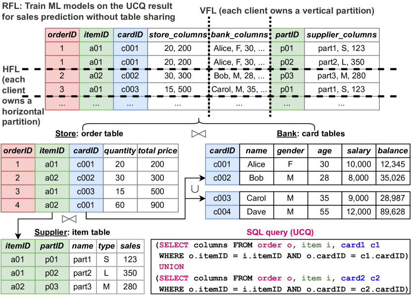
Figure 1. A RFL example, using UCQ (with SQL syntax) to express the joins and unions over three tables.

2.1. Example Scenario of RFL

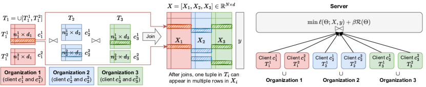
Figure 2. Illustration of RFL where the table $X$ with column $y$ is the UCQ result. Each horizontal table $T_{i}^{q}$ is owned by a client $c_{i}^{q}$.

Assume there are three organizations, a store, a supplier, and a bank, as well as the following FL task: the store wants to use both the supplier’s and the bank’s data to train a user purchase model for sales prediction. As shown in Figure 1, the store owns an order table and the supplier owns an item table, where an item contains one or multiple parts. Moreover, the bank owns a card table. To obtain the complete training data for the FL task, one needs to join the three tables order, item, and card with the join predicate

$$\textbf{order}.\textit{itemID}=\textbf{item}.\textit{itemID}\quad\textbf{and}\quad\textbf{order}.\textit{cardID}=\textbf{card}.\textit{cardID}.$$

The join columns can contain duplicates. For example, as shown in Figure 1, the order table contain multiple tuples with the same itemID or the same cardID. Consequently, the join result can be substantially larger than each individual table.

Each table involved in the join can be horizontally partitioned into multiple tables, and each horizontal table can be owned by a different client. In the example shown in Figure 1, the card table is partitioned into two tables, $\textbf{card}_{1}$ and $\textbf{card}_{2}$, that are managed by two branches of the same bank or even by two distinct banks maintaining the same schema as the original card table. This necessitates an additional union over the join results. In database literature, it can be naturally expressed as union of conjunctive queries (UCQ) (Ullman, 1988).

2.2. Problem Formalization

Assume there are $M$ organizations and the $i$-th organization consists of $Q_{i}$ clients. These $Q_{i}$ clients jointly possess a vertical table $T_{i}$, where the $q$-th client possesses a horizontal part of table $T_{i}$ denoted as $T_{i}^{q}$ and thus $T_{i}=\cup[T_{i}^{1},\dots,T_{i}^{Q_{i}}],\forall i\in[M]$. We call $T_{i}^{q}$ a horizontal table of $T_{i}$. Each $T_{i}^{q}$ contains $n_{i}^{q}$ tuples and $d_{i}$ features, and therefore $T_{i}$ contains $n_{i}=\sum_{q=1}^{Q}{n_{i}^{q}}$ tuples and $d_{i}$ features (i.e., $T_{i}\in\mathbb{R}^{n_{i}\times d_{i}}$). The total client count is $Q$, which is the sum of $Q_{i}$ across all organizations. We can perform SQL (UCQ) queries on these tables $\{T_{i}^{q}\}_{q\in[Q_{i}],i\in[M]}$, as shown in Figure 2. We assume that one of the $\{T_{i}\}_{i\in[M]}$ tables contains the label column.

We denote the entire joined table (i.e., the UCQ result) as $X=\,\bowtie[T_{1},\dots,T_{M}]=[X_{1},\dots,X_{M}]$, which contains $N$ tuples, $d=\sum_{i=1}^{M}d_{i}$ feature columns, and a label column $y\in\mathbb{R}^{N}$. A single server is responsible for coordinating these clients to jointly train machine learning models on $X$. We can now define the optimization problem associated with RFL as Eq. 1:

(1) $$\min_{\Theta}\frac{1}{N}\sum_{j=1}^{N}\ell(\Theta;X_{i,j},y_{j})+\beta\mathcal{R}(\Theta),$$

$$\text{where }X_{i,j}=\{\,\bowtie[T_{1},\dots,T_{M}]\}_{i,j},T_{i}=\cup[T_{i}^{1},\dots,T_{i}^{Q_{i}}],i\in[M].$$

Here, we assume that the server has obtained and stored the UCQ results as $X=[X_{1},\dots,X_{M}]=\{X_{i,j}\}_{i\in[M],j\in[N]}$, i.e., $X_{i,j}$ is the $j$-th tuple of $X_{i}$. In this case, we can directly train the ML models with parameters $\Theta$ on $X$ in the server. Moreover, $\ell$ represents the loss function (e.g., cross entropy loss) and $\mathcal{R}$ represents the regularization function (e.g., $L^{2}$-norm) for $\Theta$ (with constant $\beta$). In practice, clients do not share tables with the server, so the server cannot directly obtain $X$. As a result, Eq. 1 cannot be directly solved as it is.

2.3. Limitations of Existing Work

We present a brief overview of existing work on horizontal and vertical FL, and discuss its limitations for the RFL problem.

Horizontal FL (HFL) is a special case of RFL when there is only one organization (i.e., $M=1$). Each client in the organization owns a horizontal partition of a large table (McMahan et al., 2017; Konečný et al., 2016a, b). Existing work for HFL, such as FedAvg (McMahan et al., 2017), usually trains local models atop individual horizontal partitions and then synchronizes (e.g., by taking the average of) the model parameters or gradients periodically.

Vertical FL (VFL) is another special case of RFL. A single table is shared across multiple clients where each client owns a vertical partition, i.e., a set of feature columns. Moreover, it assumes that the tuples in each vertical partition can be one-to-one aligned without joins. VFL has been extensively studied (Liu et al., 2023; Cheng et al., 2021; Wu et al., 2020; Gu et al., 2020; Hardy et al., 2017; Yang et al., 2019b; Zhang et al., 2021; Feng and Yu, 2020; Hu et al., 2019a; Liu et al., 2019; Vepakomma et al., 2018; Chen et al., 2020a; Hu et al., 2019b; Jin et al., 2021), and typically leverages SGD (Liu et al., 2023; Hu et al., 2019b; Chen et al., 2020a) or ADMM (Xie et al., 2022; Hu et al., 2019a) to train local models in distributed clients.

Relational FL (RFL) is more complex than HFL and VFL, with both vertical and horizontal tables of different sizes, as well as one-to-many or many-to-many relationship introduced by joins. We cannot directly run HFL/VFL on the horizontal tables shown in Figure 2, because we cannot directly define the model objective functions for HFL/VFL on these horizontal tables (e.g., $T_{1}^{1}$ and $T_{1}^{2}$), as the model objective function is defined on the joined table. If we want to use HFL/VFL as shown in Figure 1, we need to perform the UCQ to extract the training data and then repartition the UCQ result to fit into the data layout expected by the existing HFL/VFL methods. However, it requires table sharing that is infeasible. In the rest of this paper, we present TablePuppet, a novel generic framework for RFL that generalizes HFL and VFL with SQL operations.

3. Overview of TablePuppet

The key idea of TablePuppet is to decompose the learning process involved in RFL into two steps: (1) learning over join (LoJ) followed by (2) learning over union (LoU).

Specifically, the LoJ step pushes ML on the entire joined table to each (virtual) vertical table $T_{i}$ instead of the vertical partition of the joined table. This step involves a table mapping mechanism to avoid actual joins and unions, and it employs optimization strategies that can significantly reduce the computation and communication complexities (from $\mathcal{O}(N)$ to $\mathcal{O}(n_{i})$, where $N$ is the length of the joined table and $n_{i}$ denotes the length of each vertical table $T_{i}$). For each learning problem on the vertical table $T_{i}$ resulted from the LoJ step, the LoU step further pushes ML computation to each horizontal table $T_{i}^{q}$.

TablePuppet coordinates the LoJ and LoU computation on vertical/horizontal tables using a server-client architecture (detailed in Section 4), where the server can be one of the clients or an independent instance. The global ML model with parameters $\Theta$ is partitioned into local models that are stored within individual clients. The server performs global server-side computation and coordinates the computation across clients, while clients perform client-side computation with local model updates.

Moreover, TablePuppet is a generic RFL framework in the sense that it allows for integrating with various genres of learning algorithm. We demonstrate this by illustrating how to integrate TablePuppet with two commonly used algorithms, SGD and ADMM.

Figure 3. TablePuppet framework and its training process. The red (black) locks indicate locations where DP is (can be) applied.

Table 1. Table of Notations.

Notation	Definition
$T_{i},T_{i}^{q}$	Organization $i$ owns $T_{i}$ and its $q$-th client owns $T_{i}^{q}$
$X_{i}$	The i-th vertical slice of the joined table $X$
$X_{i,j}\mapsto T_{i,p_{i}(j)}$	The $j$-th tuple of $X_{i}$ is from the $p_{i}(j)$-th tuple of $T_{i}$
$h_{i,j}=f_{i}(\theta_{i};x)$	$h_{i,j}$ is the prediction of model $f_{i}(\theta_{i})$ on tuple $x$

3.1. Learning over Join on Vertical Tables (LoJ)

LoJ first uses a table mapping mechanism to build a logical joined table $X$ to represent the UCQ result without table sharing among clients. It then decomposes/pushes learning over the joined table to each vertical table $T_{i}$. It finally performs computation and communication reduction for duplicate tuples introduced by joins.

3.1.1. Table-Mapping Mechanism

To represent the global table of UCQ results, our key idea is to join the $\langle\textit{join\_key},\textit{row\_id}\rangle$ columns of each table to get an index mapping between the logical joined table $X$ and each vertical table $T_{i}$ as $X_{i,j}\mapsto T_{i,p_{i}(j)}$, i.e., the $j$-th tuple of $X_{i}$ comes from the $p_{i}(j)$-th tuple of $T_{i}$ as shown in Figure 3(a), and $p_{i}$ denotes the mapping function for $T_{i}$. This index mapping can help us transform FL on the joined table $X$ to FL on each vertical table $T_{i}$.

Step 1: To obtain this mapping, each client first extracts the $\langle\textit{join\_key},\textit{row\_id}\rangle$ columns from its table, and then sends these columns to the server. The clients that own labels need to send the labels to the server as well. We will detail the related privacy guarantees in Section 4.3.

Step 2: After collecting $\langle\textit{join\_key},\textit{row\_id}\rangle$ columns from all the clients, the server first merges the collected $\langle\textit{join\_key},\textit{row\_id}\rangle$ of horizontal tables to be $\langle\textit{join\_key},\textit{row\_id}\rangle$ of vertical table $T_{i}$. It then joins the join_key columns specified in the UCQ and obtains the mapping $p_{i}=\left[X_{i,j}\mapsto T_{i,p_{i}(j)}\right]$ for mapping $X_{i}$ to $T_{i}$.

After that, the computation on each tuple of the joined table $X$ (i.e., $X_{i,j}$) can be transferred to the computation on the corresponding tuple of the vertical table $T_{i}$, i.e., $T_{i,p_{i}(j)}$. The server also aggregates the received labels as $y$ based on the table mapping.

3.1.2. Problem Decomposition and Push Down

LoJ aims to push ML training on the joined table $X$ down to each vertical table $T_{i}$. Inspired by the vertical FL solution (Liu et al., 2023), TablePuppet first decouples the global model to local models by partitioning global model parameters $\Theta$ to $\Theta=[\theta_{1},\dots,\theta_{M}]$, where $\theta_{i}$ is the parameter of the local model $f_{i}$ associated with $X_{i}$. Then, TablePuppet transforms the RFL problem of Eq. 1 to an optimization problem on the model prediction of each local model as Eq. 2, where $h_{i,j}$ denotes the model prediction of $f_{i}$ on tuple $X_{i,j},\forall j\in[N]$:

(2) $$\min_{\{\theta_{i}\}_{i=1}^{M}}\frac{1}{N}\sum_{j=1}^{N}\ell\left(\sum_{i=1}^{M}h_{i,j};y_{j}\right)+\beta\sum_{i=1}^{M}\mathcal{R}_{i}(\theta_{i}),$$

$$\text{where }h_{i,j}=f_{i}(\theta_{i};X_{i,j})=f_{i}(\theta_{i};T_{i,p_{i}(j)}),T_{i}=\cup[T_{i}^{1},\dots,T_{i}^{Q_{i}}].$$

Finally, we leverage the table-mapping mechanism to push the learning problem on $X_{i}$ to the corresponding vertical table $T_{i}$ with $h_{i,j}=f_{i}(\theta_{i};T_{i,p_{i}(j)}),\forall j\in[N]$, which does not require $X_{i}$ any more. In general, we can use a linear function of $\psi$ to aggregate the model predictions in the loss function $\ell$ as $\ell(\psi(h_{i,j},\dots,h_{M,j});y_{j})$. In this paper, we use summation for $\psi$ as $\ell(\psi(h_{i,j},\dots,h_{M,j});y_{j})=\ell(\sum_{i=1}^{M}h_{i,j};y_{j})$; we leave the extension to a general linear function in future work. For linear models, $\theta_{i}$ is a matrix as $\theta_{i}\in\mathbb{R}^{d_{i}\times d_{c}}$, where $d_{c}$ is the number of classes. For deep learning models, $\theta_{i}$ refers to the parameters of the neural network.

We cannot directly solve the optimization problem of Eq. 2, since the server cannot directly compute its gradient $\nabla_{\theta_{i}}\ell_{j}=\frac{\partial\ell_{j}}{\partial\theta_{i}}$ (here, $\ell_{j}=\ell(\sum_{i=1}^{M}h_{i,j};y_{j})$), which requires that both the local models and tables only reside in individual clients. To address this, we decompose this optimization problem into sub-problems and push each sub-problem to the corresponding vertical table $T_{i}$.

Specifically, we discuss below how to push SGD and ADMM down to vertical tables, alongside necessary computation on the server side. For SGD, we focus on how to break down the gradient computation across vertical tables as well as the server. For ADMM, we focus on how to decompose the global optimization problem into separate and independent optimization problems, each associated with a vertical table. Compared to decomposed gradient computation in SGD, these independent optimization problems in ADMM enable more computation on the client side, thereby reducing the communication rounds with the server:

(1) SGD. We can decompose the optimization problem of Eq. 2 into two sub-problems, by the chain rule $\nabla_{\theta_{i}}\ell_{j}=\frac{\partial\ell_{j}}{\partial h_{i,j}}\frac{\partial h_{i,j}}{\partial\theta_{i}}$. The first sub-problem is to compute the partial derivative of $\ell_{j}$ w.r.t. $h_{i,j}$ as $\frac{\partial\ell_{j}}{\partial h_{i,j}}$ on the server side, since the server can obtain all the model predictions $h_{i,j}$ from clients. The second sub-problem is to compute the partial derivative of $h_{i,j}$ w.r.t. $\theta_{i}$ as $\frac{\partial h_{i,j}}{\partial\theta_{i}}$ on the client side. Consequently, the client with $T_{i}$ can compute $\nabla_{\theta_{i}}\ell_{j}$ after receiving the $\frac{\partial\ell_{j}}{\partial h_{i,j}}$ from the server, and further compute the gradient of Eq. 2 as $\nabla_{\theta_{i}}F(T_{i})$ using Eq. 2 shown in Table 2. Finally, the client with $T_{i}$ can update its local $\theta_{i}$ using Eq. 2 with learning rate $\eta$. Now we have pushed the LoJ problem down to each vertical $T_{i}$ associated with client-side computation of Eq. 2 and Eq. 2, alongside server-side computation of Eq. 2. We can also use mini-batch SGD to perform these equations, by randomly subsampling a batch $B$ from $N$ and change $N$ to $B$ in each equation. However, the client-side computation complexity remains $\mathcal{O}(N)$.

(2) ADMM. Unlike SGD, ADMM aims to decompose the global optimization problem of Eq. 2 into multiple independent optimization sub-problems. To achieve this, we follow the sharing ADMM paradigm (Boyd et al., 2011) to rewrite Eq. 2 into the Eq. 3 below, by introducing auxiliary variables $z=\{z_{j}\}_{j=1}^{N}$ where $z_{j}\in\mathbb{R}^{d_{c}}$:

(3) $$\begin{matrix}\text{minimize }&\frac{1}{N}\sum_{j=1}^{N}\ell\left(z_{j};y_{j}\right)+\beta\sum_{i=1}^{M}\mathcal{R}_{i}(\theta_{i}),\\ \text{subject to}&\sum_{i=1}^{M}h_{i,j}-z_{j}=0,\,\,h_{i,j}=f_{i}(\theta_{i};T_{i,p_{i}(j)}).\end{matrix}$$

We then add a quadratic term to the Lagrangian of Eq. 3, known as augmented Lagrangian (Boyd et al., 2011). After that, we can solve the optimization problem using ADMM with three update steps, including the server-side $z$-update and $\lambda$-update (Eq. 2 and 2), as well as the client-side $\theta$-update (Eq. 2), as shown in Table 2. In these equations, the form of $a^{t}$ refers to the value of $a$ in the $t$-th epoch, while $\rho\in\mathbb{R}$ is a penalty parameter that can be tuned. $\{\lambda_{j}\}_{j=1}^{N}$ are dual variables and $\lambda_{j}\in\mathbb{R}^{d_{c}}$. The $\{s_{i,j}\}_{j=1}^{N}$ are residual variables for each table $T_{i}$, where $s_{i,j}=\sum_{k=1,k\neq i}^{M}f_{i}(\theta_{k};T_{k,p_{k}(j)})-z_{j}$. This decomposition pushes independent optimization problems (i.e., $\theta_{i}$-update) to each vertical table $T_{i}$, which requires less frequent communication with the server (only after the $\theta_{i}$-update finishes) compared to the (mini-batch) SGD.

Table 2. The problem decomposition for LoJ, using SGD and ADMM with computation/communication reduction.

Algorithm	Server	Client with $T_{i}$
SGD	$\begin{aligned} \frac{\partial\ell_{j}}{\partial h_{i,j}},\quad\forall j\in[N].(4)\end{aligned}$	$\begin{aligned} \nabla_{\theta_{i}}F(T_{i})&=\frac{1}{N}\sum_{j=1}^{N}\left(\frac{\partial\ell_{j}}{\partial\theta_{i}}+\beta\frac{\partial\mathcal{R}_{i}}{\partial\theta_{i}}\right),(5)\\ \theta_{i}&:=\theta_{i}-\eta\nabla_{\theta_{i}}F(T_{i}).(6)\end{aligned}$
ADMM	$\begin{aligned} z_{j}^{t}&=\operatorname*{argmin}_{z_{j}}\left(\ell\left(z_{j};y_{j}\right)-\left(\lambda_{j}^{t-1}\right)^{\top}z_{j}+\frac{\rho}{2}{\left\|\sum_{i=1}^{M}f_{i}(\theta_{i}^{t};T_{i,p_{i}(j)})-z_{j}\right\|}^{2}\right),(7)\\ \lambda_{j}^{t}&=\lambda_{j}^{t-1}+\rho\left(\sum_{i=1}^{M}f_{i}(\theta_{i}^{t};T_{i,p_{i}(j)})-z_{j}^{t}\right).(8)\end{aligned}$	$\begin{aligned} &\theta_{i}^{t+1}=\operatorname*{argmin}_{\theta_{i}}\left(\beta\mathcal{R}_{i}(\theta_{i})+\frac{1}{N}\sum_{j=1}^{N}\lambda_{j}^{t\top}f_{i}(\theta_{i};T_{i,p_{i}(j)})\right.\\ &\quad\quad\quad\quad\quad\quad\,\,\,\left.+\frac{1}{N}\sum_{j=1}^{N}\frac{\rho}{2}{\left\|s_{i,j}^{t}+f_{i}(\theta_{i};T_{i,p_{i}(j)})\right\|}^{2}\right).(9)\end{aligned}$
SGD-Opt	$\begin{aligned} Y_{i,j}&=\sum_{g\in G_{i}(j)}\frac{\partial\ell_{g}}{\partial h_{i,g}},\quad\forall j\in[n_{i}],(10)\\ G_{i,j}&=\left|G_{i}(j)\right|,\quad\forall j\in[n_{i}].(11)\end{aligned}$	$\begin{aligned} \nabla_{\theta_{i}}F(T_{i})&=\frac{1}{N}\sum_{j=1}^{n_{i}}\left(Y_{i,j}\frac{\partial h_{i,j}}{\partial\theta_{i}}+\beta G_{i,j}\frac{\partial\mathcal{R}_{i}}{\partial\theta_{i}}\right),(12)\\ \theta_{i}&:=\theta_{i}-\eta\nabla_{\theta_{i}}F(T_{i}).(13)\end{aligned}$
ADMM-Opt	$\begin{aligned} &\text{Apart from Eq.~{}\ref{Eq:z-update-unoptimized} and \ref{Eq:lambda-update-unoptimized}, the server also performs:}\\ Y_{i,j}^{t}&=\sum_{g\in G_{i}(j)}(\lambda_{g}^{t}+\rho s_{i,g}^{t}),\quad\forall j\in[n_{i}],(14)\\ G_{i,j}&=\left|G_{i}(j)\right|,\quad\forall j\in[n_{i}].(15)\end{aligned}$	$\begin{aligned} &\theta_{i}^{t+1}=\operatorname*{argmin}_{\theta_{i}}\left(\beta\mathcal{R}_{i}(\theta_{i})+\frac{1}{N}\sum_{j=1}^{n_{i}}({Y_{i,j}^{t}})^{\top}f_{i}(\theta_{i};T_{i,j})\right.\\ &\quad\quad\quad\quad\quad\quad\quad\quad\,\,\,\left.+\frac{1}{N}\sum_{j=1}^{n_{i}}\frac{\rho G_{i,j}}{2}\left\|f_{i}(\theta_{i};T_{i,j})\right\|^{2}\right).(16)\end{aligned}$

Table 3. The problem decomposition for LoU, using optimized SGD and ADMM.

Algorithm	Coordinator (Server)	Client with $T_{i}^{q}$
SGD-Opt	$\begin{aligned} \nabla_{\theta_{i}}F(T_{i})=\frac{1}{N}\sum_{q=1}^{Q_{i}}\nabla_{\theta_{i}}F(T_{i}^{q}).(17)\end{aligned}$	$\begin{aligned} \nabla_{\theta_{i}}F(T_{i}^{q})&=\sum_{j=1}^{n_{i}^{q}}\left(Y_{i,j}\frac{\partial h_{i,j}}{\partial\theta_{i}}+\beta G_{i,j}\frac{\partial\mathcal{R}_{i}}{\partial\theta_{i}}\right),(18)\\ \theta_{i}&:=\theta_{i}-\eta\nabla_{\theta_{i}}F(T_{i}).(19)\end{aligned}$
ADMM-Opt	$\begin{aligned} w_{i}^{\tau}&=\operatorname*{argmin}_{w_{i}}\left(\beta\mathcal{R}_{i}(w_{i})+\frac{M\rho}{2}{\left\|w_{i}-\overline{\theta_{i}^{\tau}}-\overline{u_{i}^{\tau-1}}\right\|}^{2}\right),(20)\\ u_{i}^{q,\tau}&=u_{i}^{q,\tau-1}+\theta_{i}^{q,\tau}-w_{i}^{\tau}.(21)\end{aligned}$	$\begin{aligned} &\theta_{i}^{q,\tau+1}=\operatorname*{argmin}_{\theta_{i}^{q}}\left(\frac{1}{N}l\left(\theta_{i}^{q};T_{i}^{q}\right)+\frac{\rho}{2}{\left\|\theta_{i}^{q}-w_{i}^{\tau}+u_{i}^{q,\tau}\right\|}^{2}\right).(22)\end{aligned}$

3.1.3. Computation and Communication Reduction

Though ADMM can reduce the communication rounds compared to SGD, its computation and communication complexity remains $\mathcal{O}(N)$ as that of SGD. Regarding the computation complexity, both SGD and ADMM need to perform $\sum_{j=1}^{N}(\cdot)$ during client-side computation using Eq. 2 and  2. Here, $N$ refers to the length of the joined table $X$, which can be orders of magnitude larger than the length of each vertical table $T_{i}$ as $n_{i}$, due to the duplicate tuples introduced by joins. For example, if both $X_{i,a}$ and $X_{i,b}$ are generated by the same tuple $T_{i,k}$ after the join, $T_{i,k}$ will be visited twice during the client-side computation of SGD and ADMM. Regarding the communication complexity, the server needs to send its computation results to each client with $T_{i}$ in each epoch, such as the partial gradient $\frac{\partial\ell_{j}}{\partial h_{i,j}}$ of SGD and the $s_{i,j}$, $\lambda_{j}$ of ADMM. These variables have the length of $N$, leading to communication complexity of $\mathcal{O}(N)$.

To minimize the computation and communication overhead, our LoJ step conducts the following two optimization strategies: (1) reduce the client-side computation on duplicate tuples by aggregating the server-side computation results (variables); and (2) communicate the aggregated variables instead of the original ones between the server and clients. Below we detail how to perform them for SGD and ADMM:

(1) SGD. After reviewing the chain rule of $\nabla_{\theta_{i}}\ell_{j}=\frac{\partial\ell_{j}}{\partial h_{i,j}}\frac{\partial h_{i,j}}{\partial\theta_{i}}$, we found that the second part $\frac{\partial h_{i,j}}{\partial\theta_{i}}$ is the same for duplicate tuples from $T_{i}$, because this part is only determined by the model function $f_{i}$ and each tuple of $T_{i}$. In this case, we can aggregate the first part for duplicate tuples on the server side, and then send the aggregated variables to the clients for reducing the client-side computation.

To facilitate the aggregation on the server side, we first construct a reverse table mapping $T_{i,j}\mapsto X_{i,G_{i}(j)}$, which means $T_{i,j}$, i.e., the $j$-th tuple of $T_{i}$, is mapped to multiple tuples in $X_{i}$, denoted as $\{X_{i,g}\}_{g\in G_{i}(j)}$. We then aggregate the $\frac{\partial\ell_{j}}{\partial h_{i,j}}$ of duplicate tuples as shown in Eq. 2 and Eq. 2. Using the aggregated variables $Y_{i,j}$ and $G_{i,j}$, we can rewrite the client-side computation of Eq. 2 into Eq. 2, where ${G}_{i}$ remains the same in each epoch.

Note that Eq. 2 has transformed the computation of $\sum_{j=1}^{N}(\cdot)$ to $\sum_{j=1}^{n_{i}}(\cdot)$ and therefore the computation overhead is reduced from $O(N)$ to $O(n_{i})$. Moreover, the server can send ${Y}_{i}\in\mathbb{R}^{n_{i}\times d_{c}}$ and $G_{i}\in\mathbb{R}^{n_{i}}$ to the client that owns $T_{i}$, instead of sending $\frac{\partial\ell_{j}}{\partial h_{i,j}}\in\mathbb{R}^{N\times d_{c}}$ and the table-mapping that are in $O(N)$. Therefore, the communication overhead between the server and the clients is reduced from $\mathcal{O}(N)$ to $\mathcal{O}(n_{i})$ as well. However, for mini-batch SGD with batch size of $B$, the server needs to perform the aggregation for the duplicate tuples inside each batch, so the reduced computation and communication is between $\mathcal{O}(n_{i})$ and $\mathcal{O}(N)$.

(2) ADMM. For the client-side computation of Eq. 2, duplicate tuples will lead to duplicate computation of $f_{i}(\theta_{i};T_{i,p_{i}(j)})$. To reduce this computation, we can perform the optimization strategy similar to SGD. The server combines and aggregates the variables (e.g., $\lambda_{j}$ and $s_{i,j}$) of duplicate tuples as shown in Eq. 2 and Eq. 2. Using $Y_{i,j}$ and $G_{i,j}$, we can rewrite the $\theta_{i}$-update as Eq. 2.

Similar with the optimization on SGD, Eq. 2 transforms the computation of $\sum_{j=1}^{N}(\cdot)$ to $\sum_{j=1}^{n_{i}}(\cdot)$ and thus reduces the computation overhead from $O(N)$ to $O(n_{i})$. Moreover, the server can send ${Y}_{i}$ and $G_{i}$ to the client that owns $T_{i}$, instead of sending $\lambda$, $s_{i}$ and the table-mapping that are in $O(N)$ as shown by Eq. 2. Therefore, the communication overhead is also reduced from $\mathcal{O}(N)$ to $\mathcal{O}(n_{i})$. More details can be found in the Appendix (App, 2024).

3.2. Learning over Union on Horizontal Tables

LoJ has pushed ML training down to each vertical table $T_{i}$. The next question is how to push the computation down to each horizontal table $T_{i}^{q}$. For SGD, we can decompose the gradient computation and synchronize it for local model update, as the gradient computation on each tuple is independent. For ADMM, to decompose the optimization problem of $\theta_{i}$-update, we can also use SGD. However, to reduce the number of communication rounds, we use horizontal ADMM instead to decompose it to independent optimization problems on horizontal tables:

(1) SGD. Our goal is to push the computation on $T_{i}$, i.e., Eq. 2 and Eq. 2, down to the clients that own $\{T_{i}^{q}\}_{q\in[Q_{i}]}$. Our key idea is to decouple the gradient computation while performing the same model update in each client as that of Eq. 2. First, we allocate the same model with the same $\theta_{i}$ for each client with $T_{i}^{q}$. Second, we decompose the gradient computation of Eq. 2 into sub-problems as follows: (1) each client first performs partial gradient computation on $T_{i}^{q}$ as Eq. 3; (2) a coordinator of the clients then aggregates the partial gradients as Eq. 3 and sends the aggregate back to the clients; (3) each client updates the model using Eq. 3. In particular, the server can act as the coordinator as well.

(2) ADMM. For ADMM, we decompose an independent optimization problem, i.e., the $\theta_{i}$-update, into sub-problems w.r.t. the $T_{i}^{q}$’s, by leveraging consensus ADMM (Boyd et al., 2011). Conceptually, this decomposition “pushes” ADMM through the union operation down to the horizontal tables. Specifically, we first rewrite Eq. 2 as Eq. 23:

(23) $$\begin{matrix}\text{minimize}\frac{1}{N}\sum_{q=1}^{Q_{i}}l\left(\theta_{i}^{q};T_{i}^{q}\right)+\beta\mathcal{R}_{i}(\theta_{i}),\\ l\left(\theta_{i}^{q};T_{i}^{q}\right)=\sum_{j=1}^{n_{i}^{q}}\left[(Y_{i,j}^{q,t})^{\top}f_{i}(\theta_{i}^{q};T_{i,j}^{q})+\frac{\rho G_{i,j}^{q}}{2}{\left\|f_{i}(\theta_{i}^{q};T_{i,j}^{q})\right\|}^{2}\right]\end{matrix}$$

Here, $\theta_{i}^{q}$ refers to the model parameters w.r.t. $T_{i}^{q}$. $T_{i,j}^{q}$ denotes the $j$-th tuple in $T_{i}^{q}$, and $Y_{i,j}^{q,t}$ refers to the $j$-th element of the $q$-th part of $Y_{i}$ in the $t$-th epoch. We then rewrite Eq. 23 as Eq. 24 by introducing auxiliary variables $w_{i}$ to approximate each $\theta_{i}^{q}$:

(24) $$\begin{matrix}\text{minimize }&\sum_{q=1}^{Q_{i}}\frac{1}{N}l\left(\theta_{i}^{q};T_{i}^{q}\right)+\beta\mathcal{R}_{i}(w_{i}),\\ \text{subject to}&\theta_{i}^{q}-w_{i}=0,\quad\forall q\in[Q_{i}].\end{matrix}$$

We can now use consensus ADMM to solve this optimization problem with three update steps (Table 3). Here, $\overline{\theta_{i}^{\tau}}$ is the average of $\{\theta_{i}^{q,\tau}\}_{q\in[Q_{i}]}$ and $\overline{u_{i}^{\tau-1}}$ is the average of $\{u_{i}^{q,\tau-1}\}_{q\in[Q_{i}]}$, where $u_{i}$ is the scaled dual variable and $\tau$ denotes the $\tau$-th epoch of the horizontal ADMM. The coordinator performs $w$-update and the $u$-update, while each client $q$ that owns $T_{i}^{q}$ can perform the $\theta_{i}^{q}$-update. During each epoch of the horizontal ADMM, each client $q$ sends its updated $\theta_{i}^{q}$ to the coordinator and the coordinator returns $w_{i}$ and $u_{i}^{q}$ to the client $q$ for model update with one round of communication.

4. Implementation of TablePuppet

TablePuppet adopts a server-client architecture (Figure 4), where the global ML model with parameters $\Theta$ is partitioned into local models with $\{\theta_{i}^{q}\}_{i\in[M],q\in[Q_{i}]}$ stored in clients. The server and clients collaboratively and iteratively train these local models. We abstract the training process as an execution plan of three physical operators (Section 4.1), which unifies the computation and communication of SGD/ADMM (Section 4.2). TablePuppet also ensures data privacy for both features and labels with differential privacy (Section 4.3).

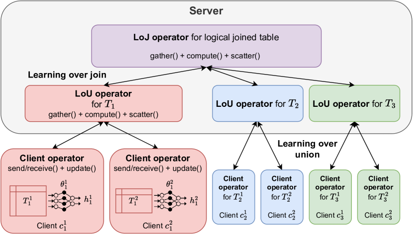
Figure 4. The architecture of TablePuppet.

4.1. Training Process with Physical Operators

We illustrate the training process in Algorithm 1. which mainly consists of two loops: (1) the outer loop that conducts learning over join (LoJ) and (2) the inner loop that performs learning over union (LoU). To implement and unify the training processes of SGD and ADMM, we design three physical operators that abstract the computation and communication of TablePuppet. The three operators include a LoJ operator, a LoU operator, and a client operator for client-side model updates. As shown in Table 4, each operator contains three functions, including a $\emph{compute}()$ for the computation, as well as $\emph{gather/scatter}()$ or $\emph{send/receive}()$ for the communication.

1

Input: Suppose $X=\bowtie[T_{1},\dots,T_{M}]$ and $T_{i}=\cup[T_{i}^{1},T_{i}^{2},\dots,T_{i}^{Q_{i}}]$. There are one server and $Q$ clients with $Q=\sum_{i=1}^{M}Q_{i}$. Each client owns a local model and a table as $T_{i}^{q}$. The number of communication rounds for outer loop is $\mathcal{T}$ and inner loop is $\mathcal{T}^{\prime}$. For SGD, $\mathcal{T}=KN/B$ and $\mathcal{T}^{\prime}=1$, where $K$ is the epoch number, $N$ is the tuple number of $X$, and $B$ is the batch size. For ADMM, $\mathcal{T}=K$.

2

3Server performs table mapping (Section 3.1.1).

4

5for communication round $t\in[\mathcal{T}]$ do  // Outer loop

6      

7      for each client with $T_{i}^{q}$, $i\in[M],q\in[Q_{i}]$ do

8            

9            computes model predictions and send them to the server.

10      Server gathers and aggregates model predictions.

11       Server does server-side computation (SGD-/ADMM-Opt in Table 2).

12       Server scatters computation results to the clients.

13      

14      for $i\in[M]$ do  // Inner loop

15             for communication round $\tau\in[\mathcal{T}^{\prime}]$  do  // $\mathcal{T}^{\prime}=1$ if $Q_{i}=1$

16                   if $Q_{i}>1$ then

17                         for each client with $T_{i}^{q}$, $q\in[Q_{i}]$ do

18                               computes and sends variables (SGD: Eq. 3 with DP, ADMM: local model parameters) to the server.

19                              

20                        Server performs coordinator-side computation (SGD: Eq. 3, ADMM: Eq. 3 and 3).

21                         Server scatters computation results to the clients.

22                        

23                  for each client with $T_{i}^{q}$, $q\in[Q_{i}]$ do

24                         performs client-side computation and model update (SGD: Eq. 3, ADMM: Eq. 3 with DP).

25                        

26                  

27            

28      

29

Algorithm 1 TablePuppet training process.

(1) LoJ operator: This operator is performed in the server for LoJ, with the assumption that each LoU operator represents a vertical table $T_{i}$. It first uses $\textit{gather}()$ to collect model predictions from each LoU operator, and then aggregates these model predictions based on the table mapping. After that, it performs server-side computation in $\textit{compute}()$. Finally, it performs $\textit{scatter}()$ to distribute the computation results to each LoU operator, as if the computation results were scattered to each $T_{i}$. As shown in Algorithm 1, the LoJ operator is responsible for the steps 5-7 of the training process.

(2) LoU operator: This operator can be performed in the server (or in each organization) as the coordinator of the clients with horizontal tables $\{T_{i}^{q}\}_{q\in[Q_{i}]}$. In the outer loop, it uses $\textit{gather}()$ to collect model predictions from clients in the same organization, and combines them as model predictions on a vertical $T_{i}$, which are sent to the LoJ operator. It also applies $\emph{scatter}()$ to distribute computation results from the LoJ operator to the clients. In the inner loop, it gathers partial gradients or variables from clients using $\textit{gather}()$, performs coordinator-side computation using $\textit{compute}()$, and distributes computation results back to clients with $\emph{scatter}()$. As shown in Algorithm 1, the LoU operator is responsible for the steps 13-14 of the training process.

(3) Client operator: This operator is performed in each client with horizontal table $T_{i}^{q}$. It applies $\emph{send}()$ to transmit model predictions, partial gradients, or model parameters to the LoU operator (coordinator) for aggregation and computation. It gets computation results, such as aggregated gradients and variables, from the LoU operator using $\emph{receive}()$. Finally, it performs $\textit{compute}()$ for model update. As shown in Algorithm 1, the client operator is responsible for the steps 4, 12, and 16 of the training process.

4.2. SGD/ADMM with TablePuppet

By combining the three physical operators in various ways and adjusting the implementations of their inner functions, we can implement SGD/ADMM not only for RFL but also for FL atop the vertical tables being joined (without the horizontal partitions). For ease of exposition, we call this special case RFL-V in the rest of this paper. As shown in Table 5, for RFL-V where each organization only has one client, we can just combine the LoJ operator and the client operator to implement RFL-SGD-V and RFL-ADMM-V. For RFL, we use all three operators with functions shown in Table 4 to implement RFL-SGD and RFL-ADMM.

Table 4. The physical operators with computation and communication functions, which cover both SGD and ADMM.

Operator	Function	SGD	ADMM
LoJ operator	gather()	model predictions	model predictions
	compute()	Eq. 2, 2	Eq. 2, 2, 2, 2
	scatter()	partial derivatives	auxiliary variables
LoU operator	gather()	model predictions,	model predictions,
		partial gradients	model parameters
	compute()	Eq. 3	Eq. 3 and Eq. 3
	scatter()	aggregated gradients	auxiliary variables
Client operator	send()	model predictions,	model predictions,
		partial gradients	model parameters
	receive()	aggregated gradients	auxiliary variables
	compute()	Eq. 3 and  3	Eq. 3

Table 5. The SGD and ADMM algorithms atop TablePuppet.

Scenario	Algorithm	Implementation of operators
RFL-V	RFL-SGD-V	LoJ: Eq. 2, 2, Client: Eq. 2, 2
	RFL-ADMM-V	LoJ: Eq. 2, 2, 2, 2, Client: Eq. 2
RFL	RFL-SGD	As that in Table 4 (SGD column)
	RFL-ADMM	As that in Table 4 (ADMM column)

4.3. Privacy Guarantees

TablePuppet introduces differential privacy (DP) (Dwork et al., 2014) to ensure data privacy for both the table features and labels. We adopt the DP definition for RFL as follows.

Definition 0 ($(\epsilon,\delta)$-DP (Dwork et al., 2014)).

A randomized algorithm $\mathcal{M}:\mathcal{X}^{n}\mapsto\Theta$ satisfies $(\epsilon,\delta)$-DP if, for every pair of neighboring datasets (i.e., the joined tables) $X,X^{\prime}\in\mathcal{X}^{n}$ that differ by one single tuple, and every possible (measurable) output set $E\subseteq\Theta$, the following inequality holds: $\operatorname{Pr}[\mathcal{M}(X)\in E]\leq e^{\epsilon}\operatorname{Pr}\left[\mathcal{M}\left(X^{\prime}\right)\in E\right]+\delta$.

We focus on addressing two key problems: (1) where to inject DP noises and (2) how to allocate the privacy budget for RFL. We present the details of our solutions below.

Noise Injection

Possible options for noise injections include the individual tables, local model parameters, or the diverse variables communicated between the server and clients, shown as black/red locks in Figure 3(b). The added noises should ensure the privacy of labels/features as well as SGD/ADMM. Our solution is to use separate DP mechanisms to safeguard labels and features, as labels are sent to the server whereas table features are kept in clients. To achieve label-level DP, we directly add noise to the raw labels (Section 4.3.1). To protect features, we perturb local model parameters on the client side (Section 4.3.2) instead of perturbing the communicated variables. Our rationale for making this design decision is that SGD and ADMM have different communicated variables so it is challenging to add noises to these variables in a uniform way. Adding noises to the local model parameters can automatically ensure DP of the communicated variables, due to the post-processing property of DP (Dwork et al., 2014).

Budget Allocation

RFL includes both LoJ and LoU that are performed on both vertical and horizontal tables and the challenge lies in how to calculate the privacy budget for this complex scenario. We allocate privacy budgets for labels and features separately: (1) For label protection, the budget is determined by the one-time noise added on raw labels (using noisy labels for training does not incur additional privacy costs due to the post-processing property of DP). (2) For feature protection, our solution is to extend the moments accountant (Abadi et al., 2016) to our framework and track the budget over multiple local training steps on each table (Section 5.2).

4.3.1. Privacy guarantee for labels

In TablePuppet, clients need to add noises to the labels before sending them to the server. Specifically, as shown by Eq. 25, TablePuppet first adds Laplace noise with per-coordinate standard deviation $\lambda$ to the labels $y$, to satisfy the DP guarantee, which results in a perturbed label vector. Then, we identify the class that retains the maximum value in the perturbed label vector as the new class label, with $N_{\mathrm{class}}$ representing the total number of classes. For continuous/numeric labels, $N_{\mathrm{class}}=1$.

(25) $$\hat{y}\leftarrow\mathrm{OneHot}(y)+\mathrm{Laplace}(\lambda),\quad\hat{y}\leftarrow\arg\max_{j\in[N_{\mathrm{class}}]}\hat{y}_{j}.$$

In addition to the labels, clients can use cryptographic methods such as SHA-256 hashing to encrypt the join_key. The server then uses the encrypted join_key to perform joins and unions, assuming that hash collision is rare.

Table 6. The computation and communication complexity comparison, where $B$ refers to the batch size and $\alpha_{i}\in[n_{i},N]$.

Complexity (Per epoch)	VFL-SGD	VFL-ADMM	RFL-SGD-V	RFL-ADMM-V	RFL-SGD	RFL-ADMM
Computation (Server)	$\mathcal{O}\left(N\right)$	$\mathcal{O}\left(N\right)$	$\mathcal{O}\left(N\right)$	$\mathcal{O}\left(N\right)$	$\mathcal{O}\left(N\right)+\mathcal{O}\left(MN/B\right)$	$\mathcal{O}\left(N\right)+\mathcal{O}\left(M\mathcal{T}^{\prime}\right)$
Computation (Client $c_{i}^{q}$)	$\mathcal{O}\left(N\right)$	$\mathcal{O}\left(N\right)$	$\mathcal{O}\left(\alpha_{i}\right)$	$\mathcal{O}\left(n_{i}\right)$	$\mathcal{O}\left(\alpha_{i}/|Q_{i}|\right)$	$\mathcal{O}\left(\mathcal{T}^{\prime}n_{i}^{q}\right)$
Communication rounds	$\mathcal{O}\left(N/B\right)$	$\mathcal{O}\left(1\right)$	$\mathcal{O}\left(N/B\right)$	$\mathcal{O}\left(1\right)$	$\mathcal{O}\left(N/B\right)$	$\mathcal{O}\left(\mathcal{T}^{\prime}\right)$
Comm. cost (Server $\leftrightarrow$ Clients)	$\mathcal{O}\left(MN\right)$	$\mathcal{O}\left(MN\right)$	$\mathcal{O}\left(\sum_{i=1}^{M}\alpha_{i}\right)$	$\mathcal{O}\left(\sum_{i=1}^{M}n_{i}\right)$	$\mathcal{O}\left(\sum_{i=1}^{M}\alpha_{i}\right)+\mathcal{O}\left(QN/B\right)$	$\mathcal{O}\left(\sum_{i=1}^{M}n_{i}+\mathcal{T}^{\prime}Q\right)$

4.3.2. Privacy guarantee for features

To protect the communicated variables as well as each client’s local data, we introduce DP-SGD (i.e., clipping and perturbing) (Abadi et al., 2016) when updating each local model so that it satisfies $(\epsilon,\delta)$-DP. Since DP holds for any post-processing on top of the data, the communicated variables based on client’s local model, such as model predictions, partial derivatives/gradients, and model parameters, also satisfy $(\epsilon,\delta)$-DP.

Specifically, when updating the local model of each client, we first clip per-sample gradient $\mathcal{G}_{j}$ with $L^{2}$-norm threshold $C$, and then add Gaussian noise sampled from $\mathcal{N}(0,\sigma^{2}C^{2})$ to the averaged batch gradient as $\mathcal{G}\leftarrow\frac{1}{B}\left(\sum_{j=1}^{B}\mathtt{Clip}\left(\mathcal{G}_{j},\mathcal{C}\right)+\mathcal{N}\left(0,\sigma^{2}\mathcal{C}^{2}\right)\right)$. Here, $\mathcal{G}_{j}$ is the gradient of the $j$-th sample/tuple, and $\mathcal{G}$ is the averaged gradient over a batch. $B$ refers to the batch size. For SGD, we perturb $\nabla_{\theta_{i}}F(T_{i})$, by performing per-sample gradient Clip in Eq. 3 with $\mathcal{G}_{j}=\frac{\partial\ell}{\partial\theta_{i}}+\beta\frac{\partial\mathcal{R}_{i}}{\partial\theta_{i}}$ and adding noise $\mathcal{N}$. For ADMM, we directly perform the formula of $\mathcal{G}$ while computing the gradient of the $\theta_{i}^{q}$-update optimization problem (Eq. 3).

5. Formal Analysis

5.1. Complexity analysis

Table 6 summarizes the computation and communication complexity of the SGD/ADMM algorithms atop TablePuppet, in comparison with traditional VFL methods (VFL-SGD and VFL-ADMM), which are hypothetically assumed to be running on the vertical partitions of the entire joined table. For simplicity, we omit the complexity analysis of the table-mapping mechanism in Table 6. We also represent the computation/communication complexity in terms of the tuple number (e.g., $N$ and $n_{i}$), since other parameters, such as feature dimension (e.g., $d_{i}$), are correlated with the tuple number.

5.1.1. VFL and RFL-V

Each organization has only one client and the client owns a vertical table. Below we analyze the complexity of VFL-SGD, VFL-ADMM, and our RFL-SGD-V, RFL-ADMM-V.

Computation complexity. The server-side computation complexity is $\mathcal{O}(N)$ per epoch for the four algorithms, since they all perform computation on the mapped model predictions with $N$ tuples. The computation complexity of each client is $\mathcal{O}(N)$ for VFL-SGD and VFL-ADMM, since they compute on vertical partitions of the joined table. Our RFL-SGD-V and RFL-ADMM-V reduces the computation complexity to $\mathcal{O}(\alpha_{i})$ and $\mathcal{O}(n_{i})$, respectively, where $\alpha_{i}\in[n_{i},N]$ (Section 3.1.3).

Communication complexity. VFL-SGD and RFL-SGD-V split the joined table into multiple batches with $\textit{batch\_size}=B$ and gathers/scatters model predictions/gradients for every batch. Therefore, the number of communication rounds is $N/B$ per epoch. The corresponding cost between the server and all clients is $O(MN)$ per epoch for VFL-SGD and is reduced to $\mathcal{O}(\sum_{i=1}^{M}\alpha_{i})$ for RFL-SGD-V. In contrast, VFL-ADMM and RFL-ADMM-V decouple the ML training problem into sub-problems and solve each sub-problem in each client. Thus, they only need to gather/scatter model predictions/variables once per epoch between the server and clients, introducing $\mathcal{O}(1)$ communication rounds. However, VFL-ADMM still suffers from $\mathcal{O}(MN)$ communication cost per epoch, while RFL-ADMM-V reduces it to $\mathcal{O}(\sum_{i=1}^{M}n_{i})$ (Section 3.1.3).

5.1.2. RFL

Each organization can have multiple clients and each client owns a horizontal table. Below we analyze the complexity of RFL-SGD and RFL-ADMM.

Computation complexity. In the outer loop of the training process, the server has $\mathcal{O}(N)$ computation complexity as it computes on the logical joined table; in the inner loop, the server acts as the coordinator for each organization to perform coordinator-side SGD/ADMM computation. For RFL-SGD, the coordinator-side computation complexity is $\mathcal{O}(1)$, which is repeated for $N/B$ times per epoch, leading to $\mathcal{O}(MN/B)$ computation complexity for all the $M$ organizations. On average, the client-side computation complexity is $\mathcal{O}\left(\alpha_{i}/|Q_{i}|\right)$. For RFL-ADMM, the coordinator-side computation complexity is also $\mathcal{O}(1)$ but is repeated for $\mathcal{T}^{\prime}$ times per epoch, leading to $\mathcal{O}\left(M\mathcal{T}^{\prime}\right)$ for all the $M$ organizations. The corresponding client-side computation complexity is $\mathcal{O}\left(\mathcal{T}^{\prime}n_{i}^{q}\right)$.

Communication complexity. In the outer loop of the training process, the server has the same number of communication rounds and cost as that in RFL-V; in the inner loop, the server (coordinator) needs to gather/scatter variables from clients in each organization. For RFL-SGD, there is only one communication round for each inner loop, leading to $\mathcal{O}\left(Q\right)$ communication cost between the server and the $Q$ clients. Since there are $N/B$ outer loops, the total communication cost of RFL-SGD is $\mathcal{O}(\sum_{i=1}^{M}\alpha_{i})+\mathcal{O}\left(QN/B\right)$. For RFL-ADMM, the number of communication rounds is $\mathcal{T}^{\prime}$ for each inner loop, leading to $\mathcal{O}\left(\mathcal{T}^{\prime}Q\right)$ communication cost between the server and the $Q$ clients. Since there is only one outer loop per epoch, its total communication cost is $\mathcal{O}\left(\sum_{i=1}^{M}n_{i}+\mathcal{T}^{\prime}Q\right)$.

5.2. Privacy Analysis

To protect the privacy of the labels stored in the server (i.e., the dataset in Definition 1 refers to the label set), we leverage the existing Laplace DP mechanism (Dwork et al., 2014) that adds one-time Laplace noise with standard deviation $\lambda$ to each coordinate of the labels before training (Malek Esmaeili et al., 2021), so that the labels satisfy $\epsilon$-label DP (with $\delta=0$).

Theorem 1.

(Privacy guarantee for labels.) Following standard Laplace mechanism ((Dwork et al., 2014)), $\epsilon$-label DP can be achieved by injecting additive Laplace noise with per-coordinate standard deviation $\lambda=\frac{2\sqrt{2}}{\epsilon}$.

To formally protect the privacy of client’s local data, when updating the local model of each client, we clip the per-sample gradient with $\ell_{2}$-norm threshold $C$ and add Gaussian noise sampled from $\mathcal{N}(0,C^{2}\sigma^{2})$. We accumulate privacy budget based on moments accountant in (Abadi et al., 2016) along with training as follows:

Theorem 2.

(Privacy guarantee for features.) There exist constants $c_{1}$ and $c_{2}$ such that, given $Q$ clients with $\tau$ local steps ($\tau=\mathcal{T}\mathcal{T}^{\prime}S$) for each client, clipping threshold $C$, noise level $\sigma$, and batch subsampling ratio $r$, for any $\epsilon\leq c_{1}r^{2}\tau$, DP version of Algorithm 1 satisfies $(\epsilon,\delta)$-DP for all $\delta\geq 0$ if we choose $\sigma\geq c_{2}\frac{r\sqrt{\tau\log(1/\delta)}}{\epsilon}$.

The proof extends the Theorem 1 in (Abadi et al., 2016) to the DP guarantee for each client in our Algorithm 1, where each client performs $\tau=\mathcal{T}\mathcal{T}^{\prime}S$ local DP-SGD steps.

6. Evaluation

We study the effectiveness and efficiency of TablePuppet, by evaluating model accuracy and performance of SGD/ADMM atop TablePuppet as well as counterparts in diverse scenarios. These scenarios include VFL/RFL-V/RFL, non-DP/DP, different network settings, as well as different ML models on a variety of datasets. We briefly summarize our evaluation methodology and main results as follows.

(1) Effectiveness (i.e., model accuracy). We regard directly training centralized (non-federated) ML models on the joined table as the baselines, and compare SGD/ADMM atop TablePuppet with these baselines in terms of model accuracy. The experiments show that SGD/ADMM atop TablePuppet can achieve comparable model accuracy to the baselines in both VFL/RFL-V and RFL scenarios. With privacy guarantee, SGD/ADMM atop TablePuppet suffers from up to 4.5% lower model accuracy than the baselines due to the noises injected into data labels and model training.

(2) Efficiency (i.e., performance). As communication is the primary bottleneck in FL (McMahan et al., 2017), our evaluation mainly focuses on the model accuracy vs. communication time among the SGD/ADMM algorithms atop TablePuppet. Compared to SGD, ADMM takes less communication time to converge to similar model accuracy. Specifically, SGD/ADMM algorithms atop TablePuppet outperform counterparts (VFL-SGD/ADMM) in terms of communication time.

6.1. Experimental setup

Table 7. The datasets and ML models used in the evaluation, where 15% of each dataset is used for model testing.

Dataset (ML Model)	Table	#Tuple	#Feature	#Class
MIMIC-III (LR)	5	[35K, 2.9M]	[2, 717]	2
Yelp (BERT-Softmax)	3	[35K, 3.2M]	[3, 775]	5
MovieLens-1M (Linear)	3	[6K, 0.9M]	[4, 52]	5
MovieLens-1M (NN)	3	[6K, 0.9M]	[4, 52]	5

6.1.1. Datasets and models

We train four linear/NN (neural network) ML models on three real-world datasets for both classification and regression tasks, as summarized in Table 7.

(1) MIMIC-III: This is a healthcare dataset with 46K patients admitted to ICUs at the BIDMC between 2001 and 2012 (MIM, 2016). We leverage the scripts in MIMIC-III Benchmarks (Harutyunyan et al., 2019; MIM, 2023) to extract 5 tables, including Patients, Admissions, Stays, Diagnoses, and Events. We perform the decompensation prediction task, which uses logistic regression (LR) to predict whether the patient’s health will rapidly deteriorate in the next 24 hours (with 0/1 label).

(2) Yelp: This Yelp dataset contains 3 core tables business, review, and user (Yel, 2023). The label column is stars in the review table, denoting the user rating of 1 to 5 for businesses. To be simple, we only use the tuples of restaurants in the business table, and obtain 3.2M reviews and ratings from 1.2M users. We first use BERT NLP model (Devlin et al., 2019) to extract 768-dimensional embeddings from review text and then use softmax regression for classification.

(3) MovieLens-1M: This dataset contains 0.9M user ratings on about 4K movies given by 6K users (Mov, 2003), including movies, ratings, and users tables. The label column is rating in the ratings table, which denotes the user rating of 1 to 5. We use both linear regression (Linear) and neural network (NN) model with a hidden layer of 16 neurons to predict the review score. If a movie has multiple genres, there are multiple tuples for this movie in the movies table.

In VFL/RFL-V, each client owns a whole table. In RFL, each table is further divided into two horizontal partitions, i.e., we have two clients in each organization.

6.1.2. Experimental settings

By following previous work on VFL (Chen et al., 2020a; Hu et al., 2019b; Vepakomma et al., 2018), we simulate VFL/RFL-V/RFL with 1 server and $Q$ clients, on a Linux machine with 16-core CPUs and 8 GPUs. The algorithms are implemented with NumPy and PyTorch. We assume that the clients are geo-distributed in US/UK, using two network settings as US-UK and US-US. US-UK refers to the speed of AWS instances between Oregon and London with 136ms latency and 0.42 Gbps bandwidth, while US-US denotes the speed between Oregon and Virginia with 67ms latency and 1.15 Gbps bandwidth (Yuan et al., 2022). We run each experiment three times and report the average value.

6.1.3. Hyperparameters

We use grid search to tune hyperparameters such as the learning rate $\eta$ for SGD and the $\rho$ for ADMM. For each dataset, we run 10 epochs for SGD/ADMM. We vary the learning rate of SGD from 0.01 to 0.5, and vary $\rho$ of ADMM from 0.1 to 2. We set the batch size of SGD to be 10K, as small batch size leads to too many communication rounds. In DP scenario, for model training with DP-SGD, we set the ($\epsilon$, $\delta$)-DP by using $\epsilon=1$, $\delta=1e$-5 (Abadi et al., 2016) with clipping threshold $C=1$. For label DP, we set the Laplace noise $\lambda=0.5$, which results in $\epsilon=5.6$ according to Theorem 1. This label DP level is consistent with existing label DP works that typically designate $\epsilon$ values between 3 and 8 (Malek Esmaeili et al., 2021; Ghazi et al., 2021). We leverage PyTorch’s DP tool Opacus (Yousefpour et al., 2021) to implement the DP and calculate the privacy budget.

6.2. Effectiveness of TablePuppet

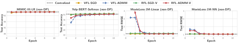
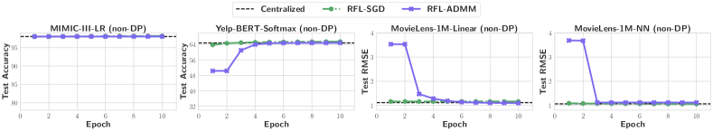
Figure 5. The convergence rates of different algorithms for VFL/RFL-V and RFL scenarios without privacy guarantees.

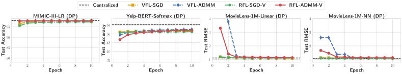
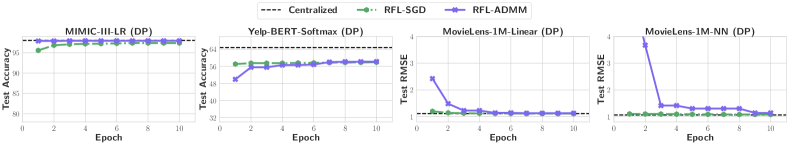
Figure 6. The convergence rates of different algorithms for VFL/RFL-V and RFL scenarios with privacy guarantees.

6.2.1. Baselines

As RFL is to train ML models on the UCQ result, we regard directly training ML models on the joined table as baselines, denoted as centralized. To obtain the baseline accuracy, we use SGD to train ML models on the joined table without privacy guarantees (shown as centralized in Figures 5 and 6). The model accuracy refers to test accuracy (higher is better) for classification models and test root mean square error (RMSE, lower is better) for regression models. We compare the model accuracy of SGD/ADMM atop TablePuppet with the baselines, as well as VFL methods (VFL-SGD/ADMM) that are forced to run directly on the vertical partitions of the joined table.

6.2.2. Results without privacy guarantee

Figure 5 illustrates the convergence rates of different SGD/ADMM algorithms without privacy guarantees. In this non-DP scenario, all the algorithms atop TablePuppet can converge to model accuracy comparable to the baselines, which demonstrates the effectiveness of TablePuppet.

For SGD algorithms, the convergence curve of RFL-SGD is similar to that of RFL-SGD-V, because they share the same gradient computation—the computation results of Eq. 3 and 3 of RFL-SGD are the same as Eq. 2 of RFL-SGD-V. Moreover, both of them exhibit comparable convergence rate to VFL-SGD, showcasing the effectiveness of our computational/communication optimization on SGD. Compared to ADMM, SGD converges faster in most cases, because SGD updates the local models much more frequently than ADMM in each epoch. For example, on the Yelp dataset, SGD updates local models 320 times (i.e., the number of batches) per epoch, whereas ADMM only updates the local model once per epoch (by completely solving the local optimization problem in each client). However, with more model updates, SGD requires more communication rounds than ADMM, leading to longer communication time per epoch (Section 6.3).

Regarding ADMM algorithms, RFL-ADMM-V achieves a similar convergence rate to VFL-ADMM. This reveals that the computation/communication optimization used by RFL-ADMM-V is effective and does not affect the convergence of ADMM. Moreover, compared to RFL-ADMM-V, RFL-ADMM demonstrates a bit lower convergence rate in the first two epochs, but catches up after two epochs on Yelp and MovieLens. We speculate the reason is that RFL-ADMM introduces more hyper-parameters, such as the number of inner loops and the $\rho$ for horizontal ADMM, which are harder to tune than RFL-ADMM-V.

6.2.3. Results with privacy guarantee

By introducing DP to both labels and model training in TablePuppet, the model accuracy of SGD/ADMM drops compared to the non-DP centralized baselines (Figure 6). Taking RFL-SGD-V for example, the test accuracy drops by 0.79 point for MIMIC-III-LR and 7.2 points for Yelp-BERT-Softmax, while the test RMSE slightly increases by 0.05 for MovieLens-Linear and 0.02 for MovieLens-NN. However, while model accuracy drops, these algorithms gain on privacy protection against feature and label leakages. In this DP scenario, we can still observe that all algorithms atop TablePuppet can converge to similar model accuracy. Specifically, SGD algorithms exhibit the fastest convergence in most cases due to the largest number of local model updates per epoch.

6.3. Efficiency of TablePuppet

We compare model accuracy vs. communication time among SGD and ADMM algorithms. We presume that the server and clients are distributed in US/UK, and we use two network setups, US-UK and US-US with different latency and bandwidth, to measure the communication between the server and clients. Due to space constraints, we only report the US-UK results here and move the US-US results, which are similar, to our GitHub repository. We measure the communication time via “latency + communication_data_size / bandwidth” for each epoch.

6.3.1. Results for VFL/RFL-V

Figure 7 illustrates the model accuracy vs. communication time in US-UK scenario, which contains two sub-figures for non-DP (top) and DP (bottom) scenarios. Each point in the figure represents the test accuracy/RMSE after one epoch. Note that VFL-SGD and RFL-SGD-V results are not fully plotted in the figure, due to the long communication time caused by too many communication rounds per epoch. For example, for the MIMIC-III dataset with 2.9M tuples, VFL-SGD suffers from 290 communication rounds per epoch, leading to extremely long communication time ($>$130 seconds for just three epochs) that exceeds the boundary of the horizontal axis. Although RFL-SGD-V outperforms VFL-SGD in terms of communication cost, it still requires the same communication rounds that leads to the long communication time. In contrast, VFL-ADMM can converge with 25s communication time, while RFL-ADMM-V only requires 6s. As another example of MovieLens-1M, RFL-ADMM-V converges with 4.3$\times$ less communication time than VFL-ADMM, owing to the communication reduction on duplicate tuples as described in Section 3.1.3. The above results are consistent with the complexity analysis in Section 5.1, where VFL-ADMM outperforms VFL-SGD due to fewer communication rounds and RFL-ADMM-V further outperforms VFL-ADMM due to less communication cost. In addition, we observe similar results in both non-DP and DP scenarios, which indicates that the privacy guarantee does not affect the number of communication rounds as well as the communication cost.

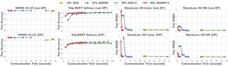
Figure 7. The model accuracy vs. communication time for VFL/RFL-V (US-UK with latency = 136ms, bandwidth = 0.42Gb/s).

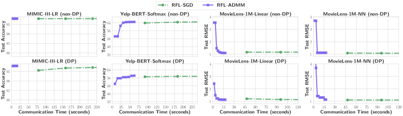
Figure 8. The model accuracy vs. communication time for RFL (US-UK with latency = 136ms, bandwidth = 0.42Gb/s).

6.3.2. Results for RFL

Figure 8 presents the model accuracy vs. communication time in US-UK scenario. Although RFL-SGD exhibits a faster convergence rate in terms of the number of epochs (Section 6.2), we can see that RFL-ADMM still takes less communication time than RFL-SGD to converge. The reason is similar to that analyzed in VFL/RFL-V, i.e., RFL-SGD requires more communication rounds due to per-batch communication as well as more communication costs due to duplicate tuples.

Compared to the results in VFL/RFL-V, SGD/ADMM algorithms for RFL require longer communication time per epoch, to communicate inner-loop computation results during LoU such as partial gradients for SGD and auxiliary variables for ADMM. Although the size of inner-loop computation results is normally smaller than that of the outer-loop computation results for LoJ, the extra inner-loop computation increases both the communication rounds and the communication cost per epoch. For example, for MovieLens-1M-Linear per epoch, the extra inner-loop communication rounds/time is 175/23.35s for RFL-SGD and 10/1.36s for RFL-ADMM, respectively. The corresponding complexity has been analyzed in Section 5.1, where RFL-SGD and RFL-ADMM require extra $\mathcal{O}(QN/B)$ and $\mathcal{O}(\mathcal{T}^{\prime}Q)$ communication cost in the inner loop. In summary, RFL-ADMM-V and RFL-ADMM outperform the others in terms of communication time.

7. Related Work

Federated Learning (FL). FL is a privacy-preserving technique for collaboratively training ML models across decentralized clients. Based on different types of data partitioning, existing surveys (Yang et al., 2019a; Liu et al., 2023) classify FL into horizontal FL, vertical FL, and federated transfer learning (FTL). Section 2.3 discussed horizontal and vertical FL, while FTL focuses on model transfer between clients using overlapping data samples and features (Liu et al., 2020; Saha and Ahmad, 2021; Chen et al., 2020b). A recent addition is hybrid FL (Zhang et al., 2020; Overman et al., 2022) where data can be partitioned both horizontally and vertically; however, existing work either requires overlapping samples/features like FTL (Zhang et al., 2020) or does not support non-convex models like neural network (Overman et al., 2022). Moreover, current FL solutions assume that the decentralized data tables can be simply one-to-one aligned, while our RFL problem targets relational tables in distributed databases that require joins and unions. FL traditionally employs training algorithms such as SGD, ADMM, block coordinate descent (BCD) (Liu et al., 2019), and gradient-boosted decision trees (GBDT) for tree-based models (Fu et al., 2021; Wu et al., 2020; Han et al., 2022). In future work, we plan to extend TablePuppet to support more types of training algorithms in addition to SGD and ADMM. To improve communication efficiency, we can also explore how to leverage asynchronous or other communication-efficient model update protocols from existing FL research (Fu et al., 2022; Xie et al., 2023; Liu et al., 2021; Gu et al., 2022).

Learning over Join. Several approaches have been proposed (Schleich et al., 2016, 2019; Kumar et al., 2015; Chen et al., 2017) for learning over joins (LoJ). However, these approaches assume that the data tables can be joined within a single machine. Moreover, these approaches suffer from either generality problems (e.g., they do not support non-polynomial loss functions well, such as logistic regression model (Schleich et al., 2016, 2019; Schleich, 2020)) or performance issues (e.g., they use standard gradient descent (GD) method that is slow to converge (Chen et al., 2017; Kumar et al., 2015; Schleich et al., 2016, 2019)). TablePuppet supports training with the more efficient (mini-batch) SGD, which converges faster than GD. TablePuppet also supports neural network models.

Privacy guarantee for FL. Different from HFL/VFL, both features and labels in RFL are distributed across clients, meaning that we need more advanced DP methods to protect them simultaneously. TablePuppet currently offers a solution by using separate label-level DP and DP-SGD to safeguard both features and labels. It remains interesting to explore how to combine these two DP methods or incorporate other advanced label-level DP mechanisms (Malek Esmaeili et al., 2021; Ghazi et al., 2021), such as post-processing the model predictions through Bayesian inference, into TablePuppet. Moreover, cryptographic techniques like homomorphic encryption (Rouhani et al., 2018; Gilad-Bachrach et al., 2016) and secure multiparty computation (Ben-Or et al., 1988; Bonawitz et al., 2017) can also be potentially added into TablePuppet to enhance its privacy guarantee, albeit with increased computation overhead.

8. Conclusion

We propose and formalize a new relational federated learning problem that aims at training ML models over relational tables with joins and unions across distributed databases. We present TablePuppet that can push two widely adopted ML training algorithms, SGD and ADMM, down to individual relational tables, with performance optimization and privacy guarantees. The SGD/ADMM algorithms based on TablePuppet can achieve model accuracy similar to centralized baseline approaches. Our ADMM algorithms also outperform others in terms of communication time.

References

- (1)
- Mov (2003) 2003. MovieLens 1M dataset. https://grouplens.org/datasets/movielens/1m/.
- GDP (2016) 2016. General Data Protection Regulation (GDPR). https://gdpr-info.eu/.
- MIM (2016) 2016. MIMIC-III Clinical Database. https://physionet.org/content/mimiciii/1.4/.
- MIM (2023) 2023. MIMIC-III Benchmarks. https://github.com/YerevaNN/mimic3-benchmarks.
- Yel (2023) 2023. Yelp Open Dataset: An all-purpose dataset for learning. https://www.yelp.com/dataset.
- App (2024) 2024. Appendix of our paper. https://github.com/JerryLead/TablePuppet/blob/master/Appendix.pdf.
- Abadi et al. (2016) Martin Abadi, Andy Chu, Ian Goodfellow, H Brendan McMahan, Ilya Mironov, Kunal Talwar, and Li Zhang. 2016. Deep learning with differential privacy. In Proceedings of the 2016 ACM SIGSAC conference on computer and communications security. 308–318.
- Ben-Or et al. (1988) Michael Ben-Or, Shafi Goldwasser, and Avi Wigderson. 1988. Completeness theorems for non-cryptographic fault-tolerant distributed computation. In Proceedings of the twentieth annual ACM symposium on Theory of computing. 1–10.
- Bonawitz et al. (2017) Keith Bonawitz, Vladimir Ivanov, Ben Kreuter, Antonio Marcedone, H Brendan McMahan, Sarvar Patel, Daniel Ramage, Aaron Segal, and Karn Seth. 2017. Practical secure aggregation for privacy-preserving machine learning. In proceedings of the 2017 ACM SIGSAC Conference on Computer and Communications Security. 1175–1191.
- Boyd et al. (2011) Stephen P. Boyd, Neal Parikh, Eric Chu, Borja Peleato, and Jonathan Eckstein. 2011. Distributed Optimization and Statistical Learning via the Alternating Direction Method of Multipliers. Found. Trends Mach. Learn. 3, 1 (2011), 1–122.
- Chen et al. (2017) Lingjiao Chen, Arun Kumar, Jeffrey F. Naughton, and Jignesh M. Patel. 2017. Towards Linear Algebra over Normalized Data. Proc. VLDB Endow. 10, 11 (2017), 1214–1225.
- Chen et al. (2020a) Tianyi Chen, Xiao Jin, Yuejiao Sun, and Wotao Yin. 2020a. Vafl: A Method of Vertical Asynchronous Federated Learning. arXiv preprint arXiv:2007.06081 (2020). arXiv:2007.06081
- Chen et al. (2020b) Yiqiang Chen, Xin Qin, Jindong Wang, Chaohui Yu, and Wen Gao. 2020b. Fedhealth: A federated transfer learning framework for wearable healthcare. IEEE Intelligent Systems 35, 4 (2020), 83–93.
- Cheng et al. (2021) Kewei Cheng, Tao Fan, Yilun Jin, Yang Liu, Tianjian Chen, Dimitrios Papadopoulos, and Qiang Yang. 2021. Secureboost: A lossless federated learning framework. IEEE Intelligent Systems 36, 6 (2021), 87–98.
- Devlin et al. (2019) Jacob Devlin, Ming-Wei Chang, Kenton Lee, and Kristina Toutanova. 2019. BERT: Pre-training of Deep Bidirectional Transformers for Language Understanding. In Proceedings of the 2019 Conference of the North American Chapter of the Association for Computational Linguistics: Human Language Technologies, NAACL-HLT 2019. 4171–4186.
- Dwork et al. (2014) Cynthia Dwork, Aaron Roth, et al. 2014. The algorithmic foundations of differential privacy. Vol. 9. Now Publishers, Inc. 211–407 pages.
- Feng and Yu (2020) Siwei Feng and Han Yu. 2020. Multi-participant multi-class vertical federated learning. arXiv preprint arXiv:2001.11154 (2020).
- Fu et al. (2022) Fangcheng Fu, Xupeng Miao, Jiawei Jiang, Huanran Xue, and Bin Cui. 2022. Towards Communication-efficient Vertical Federated Learning Training via Cache-enabled Local Update. Proc. VLDB Endow. 15, 10 (2022), 2111–2120.
- Fu et al. (2021) Fangcheng Fu, Yingxia Shao, Lele Yu, Jiawei Jiang, Huanran Xue, Yangyu Tao, and Bin Cui. 2021. VFBoost: Very Fast Vertical Federated Gradient Boosting for Cross-Enterprise Learning. In SIGMOD ’21: International Conference on Management of Data, 2021. ACM, 563–576.
- Fu et al. (2023) Rui Fu, Yuncheng Wu, Quanqing Xu, and Meihui Zhang. 2023. FEAST: A Communication-efficient Federated Feature Selection Framework for Relational Data. Proc. ACM Manag. Data 1, 1 (2023), 107:1–107:28.
- Ghazi et al. (2021) Badih Ghazi, Noah Golowich, Ravi Kumar, Pasin Manurangsi, and Chiyuan Zhang. 2021. Deep learning with label differential privacy. Advances in neural information processing systems 34 (2021), 27131–27145.
- Gilad-Bachrach et al. (2016) Ran Gilad-Bachrach, Nathan Dowlin, Kim Laine, Kristin Lauter, Michael Naehrig, and John Wernsing. 2016. Cryptonets: Applying neural networks to encrypted data with high throughput and accuracy. In International Conference on Machine Learning. PMLR, 201–210.
- Gu et al. (2020) Bin Gu, Zhiyuan Dang, Xiang Li, and Heng Huang. 2020. Federated doubly stochastic kernel learning for vertically partitioned data. In Proceedings of the 26th ACM SIGKDD International Conference on Knowledge Discovery & Data Mining. 2483–2493.
- Gu et al. (2022) Bin Gu, An Xu, Zhouyuan Huo, Cheng Deng, and Heng Huang. 2022. Privacy-Preserving Asynchronous Vertical Federated Learning Algorithms for Multiparty Collaborative Learning. IEEE Trans. Neural Networks Learn. Syst. 33, 11 (2022), 6103–6115.
- Han et al. (2022) Yujin Han, Pan Du, and Kai Yang. 2022. FedGBF: An efficient vertical federated learning framework via gradient boosting and bagging. CoRR abs/2204.00976 (2022). https://doi.org/10.48550/arXiv.2204.00976
- Hardy et al. (2017) Stephen Hardy, Wilko Henecka, Hamish Ivey-Law, Richard Nock, Giorgio Patrini, Guillaume Smith, and Brian Thorne. 2017. Private federated learning on vertically partitioned data via entity resolution and additively homomorphic encryption. arXiv preprint arXiv:1711.10677 (2017).
- Harutyunyan et al. (2019) Hrayr Harutyunyan, Hrant Khachatrian, David C. Kale, Greg Ver Steeg, and Aram Galstyan. 2019. Multitask learning and benchmarking with clinical time series data. Scientific Data 6, 1 (2019), 96.
- Hu et al. (2019a) Yaochen Hu, Peng Liu, Linglong Kong, and Di Niu. 2019a. Learning privately over distributed features: An ADMM sharing approach. arXiv preprint arXiv:1907.07735 (2019).
- Hu et al. (2019b) Yaochen Hu, Di Niu, Jianming Yang, and Shengping Zhou. 2019b. FDML: A collaborative machine learning framework for distributed features. In Proceedings of the 25th ACM SIGKDD International Conference on Knowledge Discovery & Data Mining. 2232–2240.
- Jin et al. (2021) Xiao Jin, Pin-Yu Chen, Chia-Yi Hsu, Chia-Mu Yu, and Tianyi Chen. 2021. Catastrophic Data Leakage in Vertical Federated Learning. Advances in Neural Information Processing Systems 34 (2021).
- Khan et al. (2022) Afsana Khan, Marijn ten Thij, and Anna Wilbik. 2022. Vertical Federated Learning: A Structured Literature Review. CoRR abs/2212.00622 (2022). https://doi.org/10.48550/arXiv.2212.00622
- Konečný et al. (2016a) Jakub Konečný, H. Brendan McMahan, Daniel Ramage, and Peter Richtárik. 2016a. Federated Optimization: Distributed Machine Learning for On-Device Intelligence. CoRR abs/1610.02527 (2016). arXiv:1610.02527 http://arxiv.org/abs/1610.02527
- Konečný et al. (2016b) Jakub Konečný, H. Brendan McMahan, Felix X. Yu, Peter Richtárik, Ananda Theertha Suresh, and Dave Bacon. 2016b. Federated Learning: Strategies for Improving Communication Efficiency. CoRR abs/1610.05492 (2016). arXiv:1610.05492 http://arxiv.org/abs/1610.05492
- Kumar et al. (2015) Arun Kumar, Jeffrey F. Naughton, and Jignesh M. Patel. 2015. Learning Generalized Linear Models Over Normalized Data. In Proceedings of the 2015 ACM SIGMOD International Conference on Management of Data. ACM, 1969–1984.
- Li et al. (2022) Qinbin Li, Yiqun Diao, Quan Chen, and Bingsheng He. 2022. Federated Learning on Non-IID Data Silos: An Experimental Study. In 38th IEEE International Conference on Data Engineering, ICDE 2022. IEEE, 965–978.
- Liu et al. (2021) Junxu Liu, Jian Lou, Li Xiong, Jinfei Liu, and Xiaofeng Meng. 2021. Projected Federated Averaging with Heterogeneous Differential Privacy. Proc. VLDB Endow. 15, 4 (2021), 828–840.
- Liu et al. (2020) Yang Liu, Yan Kang, Chaoping Xing, Tianjian Chen, and Qiang Yang. 2020. A secure federated transfer learning framework. IEEE Intelligent Systems 35, 4 (2020), 70–82.
- Liu et al. (2019) Yang Liu, Yan Kang, Xinwei Zhang, Liping Li, Yong Cheng, Tianjian Chen, Mingyi Hong, and Qiang Yang. 2019. A communication efficient collaborative learning framework for distributed features. arXiv preprint arXiv:1912.11187 (2019).
- Liu et al. (2023) Yang Liu, Yan Kang, Tianyuan Zou, Yanhong Pu, Yuanqin He, Xiaozhou Ye, Ye Ouyang, Ya-Qin Zhang, and Qiang Yang. 2023. Vertical Federated Learning: Concepts, Advances and Challenges. CoRR abs/2211.12814 (2023). https://doi.org/10.48550/arXiv.2211.12814 arXiv:2211.12814
- Malek Esmaeili et al. (2021) Mani Malek Esmaeili, Ilya Mironov, Karthik Prasad, Igor Shilov, and Florian Tramer. 2021. Antipodes of label differential privacy: Pate and alibi. Advances in Neural Information Processing Systems 34 (2021), 6934–6945.
- McMahan et al. (2017) Brendan McMahan, Eider Moore, Daniel Ramage, Seth Hampson, and Blaise Agüera y Arcas. 2017. Communication-Efficient Learning of Deep Networks from Decentralized Data. In Proceedings of the 20th International Conference on Artificial Intelligence and Statistics, AISTATS 2017, Vol. 54. PMLR, 1273–1282.
- Overman et al. (2022) Tom Overman, Garrett Blum, and Diego Klabjan. 2022. A Primal-Dual Algorithm for Hybrid Federated Learning. CoRR abs/2210.08106 (2022). https://doi.org/10.48550/arXiv.2210.08106
- R. et al. (2019) Santiago S. Silva R., Boris A. Gutman, Eduardo Romero, Paul M. Thompson, André Altmann, and Marco Lorenzi. 2019. Federated Learning in Distributed Medical Databases: Meta-Analysis of Large-Scale Subcortical Brain Data. In 16th IEEE International Symposium on Biomedical Imaging, ISBI 2019. IEEE, 270–274.
- Rouhani et al. (2018) Bita Darvish Rouhani, M Sadegh Riazi, and Farinaz Koushanfar. 2018. DeepSecure: Scalable provably-secure deep learning. In Proceedings of the 55th Annual Design Automation Conference. 1–6.
- Saha and Ahmad (2021) Sudipan Saha and Tahir Ahmad. 2021. Federated transfer learning: Concept and applications. Intelligenza Artificiale 15, 1 (2021), 35–44.
- Sandha et al. (2019) Sandeep Singh Sandha, Wellington Cabrera, Mohammed Al-Kateb, Sanjay Nair, and Mani B. Srivastava. 2019. In-database Distributed Machine Learning: Demonstration using Teradata SQL Engine. Proc. VLDB Endow. 12, 12 (2019), 1854–1857.
- Schleich (2020) Maximilian-Joel Schleich. 2020. Structure-aware machine learning over multi-relational databases. Ph.D. Dissertation. University of Oxford, UK. https://ethos.bl.uk/OrderDetails.do?uin=uk.bl.ethos.808366
- Schleich et al. (2016) Maximilian Schleich, Dan Olteanu, and Radu Ciucanu. 2016. Learning Linear Regression Models over Factorized Joins. In Proceedings of the 2016 International Conference on Management of Data, SIGMOD Conference 2016. ACM, 3–18.
- Schleich et al. (2019) Maximilian Schleich, Dan Olteanu, Mahmoud Abo Khamis, Hung Q. Ngo, and XuanLong Nguyen. 2019. A Layered Aggregate Engine for Analytics Workloads. In Proceedings of the 2019 International Conference on Management of Data, SIGMOD Conference 2019. ACM, 1642–1659.
- Shoham and Rappoport (2023) Ofir Ben Shoham and Nadav Rappoport. 2023. Federated Learning of Medical Concepts Embedding using BEHRT. CoRR abs/2305.13052 (2023). https://doi.org/10.48550/arXiv.2305.13052
- Ullman (1988) Jeffrey D. Ullman. 1988. Principles of Database and Knowledge-Base Systems, Volume I. Computer Science Press.
- Vepakomma et al. (2018) Praneeth Vepakomma, Otkrist Gupta, Tristan Swedish, and Ramesh Raskar. 2018. Split learning for health: Distributed deep learning without sharing raw patient data. arXiv preprint arXiv:1812.00564 (2018).
- Wu et al. (2020) Yuncheng Wu, Shaofeng Cai, Xiaokui Xiao, Gang Chen, and Beng Chin Ooi. 2020. Privacy preserving vertical federated learning for tree-based models. Proceedings of the VLDB Endowment 13, 12 (2020), 2090–2103.
- Xie et al. (2022) Chulin Xie, Pin-Yu Chen, Ce Zhang, and Bo Li. 2022. Improving Privacy-Preserving Vertical Federated Learning by Efficient Communication with ADMM. CoRR abs/2207.10226 (2022). https://doi.org/10.48550/arXiv.2207.10226
- Xie et al. (2023) Yuexiang Xie, Zhen Wang, Dawei Gao, Daoyuan Chen, Liuyi Yao, Weirui Kuang, Yaliang Li, Bolin Ding, and Jingren Zhou. 2023. FederatedScope: A Flexible Federated Learning Platform for Heterogeneity. Proc. VLDB Endow. 16, 5 (2023), 1059–1072.
- Yang et al. (2019a) Qiang Yang, Yang Liu, Tianjian Chen, and Yongxin Tong. 2019a. Federated Machine Learning: Concept and Applications. ACM Trans. Intell. Syst. Technol. 10, 2 (2019), 12:1–12:19. https://doi.org/10.1145/3298981
- Yang et al. (2019b) Shengwen Yang, Bing Ren, Xuhui Zhou, and Liping Liu. 2019b. Parallel distributed logistic regression for vertical federated learning without third-party coordinator. arXiv preprint arXiv:1911.09824 (2019).
- Yousefpour et al. (2021) Ashkan Yousefpour, Igor Shilov, Alexandre Sablayrolles, Davide Testuggine, Karthik Prasad, Mani Malek, John Nguyen, Sayan Ghosh, Akash Bharadwaj, Jessica Zhao, Graham Cormode, and Ilya Mironov. 2021. Opacus: User-Friendly Differential Privacy Library in PyTorch. CoRR abs/2109.12298 (2021). arXiv:2109.12298 https://arxiv.org/abs/2109.12298
- Yuan et al. (2022) Binhang Yuan, Yongjun He, Jared Quincy Davis, Tianyi Zhang, Tri Dao, Beidi Chen, Percy Liang, Christopher Ré, and Ce Zhang. 2022. Decentralized Training of Foundation Models in Heterogeneous Environments. CoRR abs/2206.01288 (2022). https://doi.org/10.48550/arXiv.2206.01288 arXiv:2206.01288
- Zhang et al. (2021) Qingsong Zhang, Bin Gu, Cheng Deng, and Heng Huang. 2021. Secure Bilevel Asynchronous Vertical Federated Learning with Backward Updating. In Proceedings of the AAAI Conference on Artificial Intelligence, Vol. 35. 10896–10904.
- Zhang et al. (2020) Xinwei Zhang, Wotao Yin, Mingyi Hong, and Tianyi Chen. 2020. Hybrid Federated Learning: Algorithms and Implementation. CoRR abs/2012.12420 (2020). https://arxiv.org/abs/2012.12420