Graph Image Prior for Unsupervised Dynamic MRI Reconstruction

Abstract

The inductive bias of the convolutional neural network (CNN) can act as a strong prior for image restoration, which is known as the Deep Image Prior (DIP). In recent years, DIP has been utilized in unsupervised dynamic MRI reconstruction, which adopts a generative model from the latent space to the image space. However, existing methods usually utilize a single pyramid-shaped CNN architecture to parameterize the generator, which cannot effectively exploit the spatio-temporal correlations within the dynamic data. In this work, we propose a novel scheme to exploit the DIP prior for dynamic MRI reconstruction, named “Graph Image Prior” (GIP). The generative model is decomposed into two stages: image recovery and manifold discovery, which is bridged by a graph convolutional network to exploit the spatio-temporal correlations. In addition, we devise an ADMM algorithm to alternately optimize the images and the network parameters to further improve the reconstruction performance. Experimental results demonstrate that GIP outperforms compressed sensing methods and unsupervised methods over different sampling trajectories, and significantly reduces the performance gap with the state-of-art supervised deep-learning methods. Moreover, GIP displays superior generalization ability when transferred to a different reconstruction setting, without the need for any additional data.

Dynamic MRI reconstruction, unsupervised learning, deep image prior.

1 Introduction

Dynamic magnetic resonance imaging (MRI) is one of the most challenging problems in the field of radiology, which is constrained by the trade-off between spatial resolution and temporal resolution. To break this limit, a typical approach is to accelerate the data acquisition by skipping a part of the k-space measurements. However, k-space undersampling will lead to aliasing artifacts, which need to be removed by appropriate reconstruction algorithms.

Over the past decades, reconstructing dynamic images from undersampled measurements has been one of the most investigated topics in MRI. Many methods have been proposed to exploit the spatio-temporal redundancy within the dynamic data, including the k-t space parallel imaging methods[1], linear subspace methods[2], sparsity-based methods[3][4], low-rank plus sparse methods[5][6][7], manifold-learning methods[8][9], and many others. These methods rely on hand-crafted priors for regularizing the iterative reconstruction algorithm. The reconstruction performance is highly limited by the accuracy of the priors.

In recent years, supervised deep learning methods have shown great potential for dynamic MRI reconstruction[10][11]. Given a fully sampled dataset for training, supervised learning methods can learn to remove the aliasing artifacts and reconstruct high-quality images. Besides, deep unrolling networks mark a great advance for MRI reconstruction[12][13][14]. Deep unrolling methods unfold an optimization algorithm into a fixed number of iterations, alternating between the data consistency and network regularization layers[15][16][17]. Learnable network layers can also be used to enhance the traditional regularization priors, such as sparsity[18] and low-rankness[19][20], which significantly improves the reconstruction performance and interpretability. However, supervised methods require a ground-truth dataset for training, which is not always available. Besides, supervised methods often have concerns about their generalization ability.

To address these challenges, unsupervised deep-learning methods have gained increasing research focus. Recently, it is discovered that an untrained convolutional neural network (CNN) can act as a strong regularizer for image restoration, which is known as the “Deep Image Prior” (DIP)[21]. DIP is soon used in inverse problems[22][23], and inspires several unsupervised methods for dynamic MRI reconstruction[24][25][26]. These methods generally adopt a generative model, which maps the latent variables to dynamic images. The mapping function is parameterized by a CNN, which is trained with the undersampled k-space data.

However, existing unsupervised dynamic MRI reconstruction algorithms based on DIP have some limitations. Firstly, they usually utilize a single pyramid-shaped CNN architecture to parameterize the generator. Since the convolution kernels are shared by all frames, the data correlations are totally embedded in the low-dimensional latent variables, which is disadvantageous for fully exploiting the spatio-temporal redundancies within the dynamic image. Secondly, they usually solve the model by simply fitting the undersampled k-space data, which often encounters difficulties during training and does not always converge to an optimal solution. Lastly, existing methods mainly focus on the reconstruction problem of free-breathing or un-gated cardiac imaging. However, since high-quality ground-truth images are unavailable for these applications, they usually lack the comparison with supervised deep-learning algorithms, which makes it difficult to evaluate the development status of unsupervised methods.

In this work, we propose a novel unsupervised learning model for dynamic MRI reconstruction, named “Graph Image Prior” (GIP). GIP decomposes the generative process into two stages: image recovery and manifold discovery. For the image recovery stage, independent small CNNs are used to recover the image structures for each frame. For the manifold discovery stage, the frames are considered as vertices embedded on a smooth manifold. A graph convolutional network (GCN) is adopted to exploit the spatio-temporal correlations. In addition, we devised an ADMM algorithm to enhance the reconstruction performance of GIP, which alternately optimizes the dynamic images and network parameters. The proposed method was validated on two public cardiac cine datasets. Thorough experiments were conducted to compare the proposed method with several compressed-sensing (CS) methods, unsupervised methods, and supervised deep-learning methods. Our contributions can be summarized as follows:

• This work proposes a new scheme to exploit the structural prior of CNN for unsupervised dynamic MRI reconstruction. The generative process is decomposed into two stages, bridged by a graph-structured manifold model.

• A GCN is adopted to exploit the spatio-temporal correlations. To the best of our knowledge, this work represents the first study applying the GCN to unsupervised dynamic MRI reconstruction.

• An ADMM algorithm is devised to alternately optimize the network and images. We demonstrate by experiments that the proposed optimization algorithm can significantly improve the reconstruction performance, compared with directly fitting the k-space data.

• Experimental results demonstrate that GIP outperforms the CS methods and unsupervised methods, and significantly reduces the performance gap with the state-of-art supervised deep-learning methods. Moreover, GIP displays superior generalization ability when it is transferred to a different reconstruction setting.

2 Background

2.1 Dynamic MRI Reconstruction based on DIP

The dynamic MRI acquisition can be modeled as:

$$y=Ax+\epsilon,$$ (1)

where $x\in\mathbb{C}^{N_{x}\times N_{y}\times N_{t}}$ denotes the dynamic MRI images, in which $N_{x}$ and $N_{y}$ are the image height and width, $N_{t}$ is the number of time frames. $y\in\mathbb{C}^{N_{s}\times N_{c}\times N_{t}}$ is the multi-coil undersampled k-space data, in which $N_{s}$ is the number of sample points per frame, $N_{c}$ is the number of coils. $\epsilon\in\mathbb{C}^{N_{s}\times N_{c}\times N_{t}}$ denotes the measurement noise. $A=F_{u}S$ is the multi-coil dynamic MRI system matrix, $S$ is the coil sensitivity maps, and $F_{u}$ is the undersampled Fourier transform.

In the generative model based on DIP, the dynamic images $x$ are considered to be generated from a latent variable $z$:

$$x=G_{\theta}(z),$$ (2)

where $G_{\theta}$ is a CNN network with learnable parameters $\theta$.

Previous studies usually formulate the generative model in an end-to-end manner. Yoo proposed the time-dependent DIP model (TDIP)[24], which uses a hand-crafted variable as $z$ and utilizes random batch sampling for network optimization. Zou proposed the generative SToRM model (Gen-SToRM)[25], which designs a regularization term to penalize the manifold distance of the generator output, and optimize the latent variable $z$ with the generator simultaneously. Ahmed proposed the deep bi-linear model (DEBLUR)[26], which factorizes the dynamic images into a spatial basis and a temporal basis, and uses two CNNs to generate them respectively.

2.2 Graph-Structured Manifold Model

The graph-structured manifold model was first introduced into dynamic MRI reconstruction as the SToRM model[8]. SToRM models the dynamic frames as vertices on a smooth manifold, which is parameterized by an undirected graph. The manifold smoothness is enforced by penalizing the weighted distance of neighboring vertices in the graph:

$$\min_{x}\,\,\frac{1}{2}\left\|Ax-y\right\|_{2}^{2}+\lambda\,\text{trace}\left(xLx^{H}\right),$$ (3)

where $L$ is the graph Laplacian matrix, which is estimated by the navigator signals. Subsequent studies have proposed an improved SToRM model, which exploits the local correlations to model the manifold, without the need for navigator acquisition[27]. Besides, the kernel techniques[28], sparsity priors[29] were also introduced to the graph-structured manifold model.

2.3 Graph Convolutional Networks

Graph neural networks are proposed to handle data in non-Euclidean space. Generally, a graph can be represented as $G=(V,E,X)$, where $V$ is the set of vertices or nodes, $E$ is the set of edges, and $X$ is the node feature matrix. “Graph convolution” indicates updating the node features by taking the weighted average of the information from the node’s neighbors[30]. Early works adopted the spectral-based method to perform graph convolution, which applies the filter in the graph Fourier space[31]. However, spectral-based methods need to perform eigenvalue decomposition to the graph Laplacian matrix, which is inflexible and computationally expensive[32]. Recently, spatial-based methods have become more popular, directly utilizing the graph adjacent matrix to perform graph convolution[33][34][35]. A graph convolution layer consists of a graph aggregate function and a graph update function:

$$G^{\prime} =GraphConv(G,\,W_{agg},\,W_{upd})$$ (4)

$$=Update(Aggregate(G,\,W_{agg}),\,W_{upd}),$$

where $W_{agg}$ and $W_{upd}$ denote the learnable weights.

At present, there is very limited research utilizing the GCN for MRI reconstruction. Feng proposed to use the GCN to substitute the GRAPPA kernel for highly undersampled magnetic resonance fingerprinting reconstruction[36]. However, how to use GCN in more general MRI reconstruction applications remains a problem worth further research.

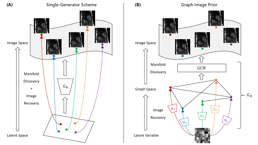
Figure 1: The conceptual model for the single-generator scheme (A) and Graph Image Prior (B). For the single-generator scheme, very low-dimensional latent variables are usually used to retain the temporal correlations. A single deep CNN architecture is utilized to directly map the latent variables to image frames in an end-to-end fashion. In comparison, GIP divides the generative process into two stages. Firstly, independent small CNNs are used to recover the spatial structure for each frame, starting from a noise input. Then, each frame is considered as a node embedded in the graph space. A GCN is used to exploit the spatio-temporal correlations, and finally output the dynamic images.

3 Methodology

3.1 Graph Image Prior Model

In concept, the generative model for unsupervised dynamic MRI reconstruction should be able to address two tasks. The first is “image recovery”, which indicates recovering the image spatial structures from the latent variable. The second is “manifold discovery”, which indicates exploiting the spatio-temporal redundancies and finding the best manifold embedding. Existing works usually adopt the single-generator scheme to address these two tasks in an end-to-end fashion, as shown in  Figure 1(A). The image structural prior and the manifold topology are both learned implicitly within the CNN weights. The two tasks are entangled with each other, which may reduce the model’s interpretability and performance.

Inspired by the SToRM model[8], we propose a novel Graph Image Prior (GIP) model as a better scheme for generative dynamic MRI representation, as shown in  Figure 1(B). First, independent small CNNs ($G_{1},\ldots,G_{N}$) are used to recover the image structure for each time frame from a single 2D noise input. Second, each frame is considered as a node embedded on the graph-structured manifold. A GCN is used to exploit the spatio-temporal correlations, and finally output the dynamic images. The independent CNNs and the GCN constitute the overall generator $G_{\theta}$.

3.2 Generator Structure

The structure of $G_{\theta}$ is illustrated in  Figure 2. In this figure, the image size is marked by purple and the channel number is marked by blue on the right side of the intermediate variables. For simplicity, we use $N$ to indicate the image of size $N\times N$. A hyper-parameter $C$ is used to control the model capacity.  Figure 2(A) displays the independent CNNs ($G_{1},\ldots,G_{N}$). A 2D noise input of size $8\times 8$ and $C_{z}$ channels is used as the latent variable, which is input into the CNNs to recover the image size for each frame.  Figure 2(B) illustrates the GCN network, which is composed of three learnable blocks: the feature extraction network (FEN), the graph aggregate layer (GAL), and the graph update layer (GUL), as shown in (C), (D), and (E), respectively. Since the graph structure is unknown before reconstruction, the FEN is used to obtain low-dimensional node features to estimate the neighborhood relationship. Cosine-similarity matrix is calculated between the node features, and the k-nearest-neighbor (kNN) algorithm is adopted for clustering the neighbors and producing the graph adjacent matrix. Next, the unordered nodes generated from the independent CNNs are connected into the input graph, where the number of vertices equals the number of frames. Then, the GAL is used to synthesize the neighborhood information for each node, which establishes a hidden graph containing the aggregated features. Finally, the GUL receives both the input graph and the hidden graph to update the features for each graph node. At the output layer of GUL, the channel number is reduced to $2$, which corresponds to the real and imaginary part of a complex-valued dynamic image.

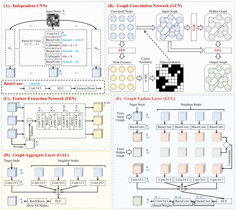
Figure 2: The network architecture of $G_{\theta}$, where the image size of the variables is marked by purple and the channel number is marked by blue. For simplicity, we use $N$ to indicate the image of size $N\times N$. $C_{z}$ is the channel number of the input latent variable. $C$ is a hyper-parameter which controls the model capacity. (A) displays the independent CNNs ($G_{1},\ldots,G_{N}$). (B) illustrates the GCN network, which is composed of three learnable blocks: the feature extraction network (FEN), the graph aggregate layer (GAL), and the graph update layer (GUL), as shown in (C), (D), and (E), respectively. The latent variable is first recovered to the image size for each frame by the independent CNNs. Then the GCN is utilized to adaptively determine the graph structure and exploit the spatio-temporal correlations. $G_{\theta}$ outputs the dynamic images of size $N$ with 2 channels, which correspond to the real and imaginary part.

3.3 Optimization Algorithm

Although the GIP generator is effective for exploiting the spatio-temporal correlations, its reconstruction performance may be limited by the strong structural bias of CNN. Inspired by Lu’s work[37], we devise an ADMM algorithm to alternately optimize the dynamic images and the network parameters to further improve the reconstruction performance.

We first consider the following optimization problem:

$$\min_{x,\theta}\,\,\,\,\frac{1}{2}\left\|Ax-y\right\|_{2}^{2},\,\,\,\,\,\,\,\,\,\,\,\,s.t.\,\,x=G_{\theta}(z),\vspace{-2.0pt}$$ (5)

where $G_{\theta}$ denotes GIP generator, $z$ denotes the latent variable.

Then, we form the augmented Lagrangian associated with  Equation 5 as follows:

$$\min_{x,\theta}\,\,\,\,\frac{1}{2}\left\|Ax-y\right\|_{2}^{2}+\frac{\rho}{2}\left\|x-G_{\theta}(z)\right\|_{2}^{2}+\textbf{Re}(<\Lambda,\,\,x-G_{\theta}(z)>),\vspace{-2.0pt}$$ (6)

where $\rho$ denotes the relaxation coefficient, $\Lambda$ is the Lagrangian multiplier, $\textbf{Re}(\cdot)$ denotes taking the real part.

Next, we adopt the ADMM algorithm to solve  Equation 6:

$$x^{(k+1)} =\min_{x}\,\,\,\,\frac{1}{2}\left\|Ax-y\right\|_{2}^{2}+\frac{\rho}{2}\left\|x-G_{\theta^{(k)}}(z)\right\|_{2}^{2}$$ (7)

$$+\textbf{Re}(<\Lambda^{(k)},\,\,x-G_{\theta^{(k)}}(z)>),$$

$$\theta^{(k+1)} =\min_{\theta}\,\,\,\,\frac{\rho}{2}\left\|x^{(k+1)}-G_{\theta}(z)\right\|_{2}^{2}$$

$$+\textbf{Re}(<\Lambda^{(k)},\,\,x^{(k+1)}-G_{\theta}(z)>),$$

$$\Lambda^{(k+1)} =\Lambda^{(k)}+\rho(x^{(k+1)}-G_{\theta^{(k+1)}}(z)).$$

Note that the first step has a closed-form solution by taking the derivative to zero. And the second step is a quadratic form for $G_{\theta}(z)$. The algorithm can be further simplified to:

$$x^{(k+1)} =(A^{H}A+\rho I)^{-1}(A^{H}y+\rho G_{\theta^{(k)}}(z)-\Lambda^{(k)}),$$ (8)

$$\theta^{(k+1)} =\min_{\theta}\,\,\,\,\left\|G_{\theta}(z)-(x^{(k+1)}+\frac{1}{\rho}\Lambda^{(k)})\right\|_{2}^{2},$$

$$\Lambda^{(k+1)} =\Lambda^{(k)}+\rho(x^{(k+1)}-G_{\theta^{(k+1)}}(z)).$$

For the first step, we adopt conjugate-gradient descent (CG) to solve the linear equation. The second step is a minimization problem about the generator output, which can be solved by network training using the back-propagation algorithm.

The network initialization is critical to the optimization performance. In this work, we adopt the “DIP initialization”, which is obtained by fitting the undersampled k-space data:

$$\min_{\theta}\,\,\,\,\left\|AG_{\theta}(z)-y\right\|_{2}^{2}.\vspace{-5.0pt}$$ (9)

In summary, we first solve  Equation 9 to initialize $G_{\theta}$. The best graph adjacent matrix is determined and fixed after the initialization. Then,  Equation 8 is implemented to fine-tune the parameters and enhance the reconstruction performance.

4 Experimental Setups

4.1 Dataset and Preprocessing

Two public cardiac MRI datasets were used in this work.

The first is the Ohio OCMR dataset[38]. A total of 76 fully sampled dynamic data slices from 43 different subjects were included in the experiment dataset. The coil number is compressed to 8 by the GCC algorithm[39]. The slices are all cropped to the image size $192\times 144$. We divided the data into three groups: 60 slices for training, 6 slices for validation, and 10 slices for testing. Besides, we applied data augmentation by cropping the slices to image size $144\times 144$ at stride $12$, which finally produced 300 slices for training, 30 slices for validation, and 50 slices for testing.

The second is the Siemens CMRxRecon dataset[40]. It contains 119 fully sampled multi-coil cardiac MRI cases. Each data has 12 frames and 10 coils. For each case, the central 3 slices at the middle position are included in the experiment dataset, which produces 357 dynamic slices. We cropped the image size to $192\times 192$, and divided the data into 240 slices for training, 30 slices for validation, and 87 slices for testing.

The ESPIRiT algorithm[41] was used to calculate the coil sensitivity maps. A $32\times 32$ block at the center of the time-averaged k-space data (ACS data) is used for calibration.

4.2 Algorithms and Experimental Details

In this work, we implemented two CS methods (L+S[7] and k-t SLR[6]), four supervised deep-learning methods (CRNN[16], SLR-net[19], CTF-net[17] and L+S-net[20]), and two unsupervised deep-learning methods (TDIP[24] and Gen-SToRM[25]) for comparison. All methods were implemented according to the source code provided by the authors. However, since the view-sharing strategy is not compatible with Cartesian sampling, the training strategy of TDIP and Gen-SToRM needs necessary modifications. To ensure a reliable comparison, we adopted the training strategy suggested by the authors, making the minimum changes to adapt the algorithms to arbitrary sampling patterns. For TDIP, we use random batch sampling among the time frames to train the generator, instead of sampling from all possible sliding windows[24]. For Gen-SToRM, we adopt a two-stage progressive training-in-time approach[25], which first initializes the generator by fitting the time-averaged k-space data and then fine-tune the parameters by training on the undersampled dynamic data.

For the supervised deep-learning methods, we directly used the default network architecture released by the authors. All the supervised methods were trained on the OCMR training set by the Adam optimizer with a learning rate $lr$=$5\times 10^{-4}$ and $\beta$=$(0.9,0.999)$. The mean squared error was used as the loss function. Random patch sampling is adopted along the time dimension to generate training samples of size $144\times 144\times 20$. 100 epochs were used for training to ensure complete convergence. Validation was performed after each epoch and the best model on the validation set was saved for testing. The trained model was tested by reconstructing a dynamic slice without temporal patch sampling.

For the CS methods and unsupervised methods, we adjusted their parameters on the OCMR validation set to ensure their best performance. For TDIP, we adopted the “Helix (L=3) + MapNet (L=64)” as the latent space design, which was reported to achieve the best performance[24]. For Gen-SToRM, we fixed the latent dimension $l(z)=2$ and model parameter $d=24$ as suggested by the authors[25].

The reconstruction methods were implemented in PyTorch on an Ubuntu 20.04 LTS operating system equipped with 8 NVIDIA A800 GPUs. Our code will be available at https://github.com/lizs17/GIP_Cardiac_MRI upon publication.

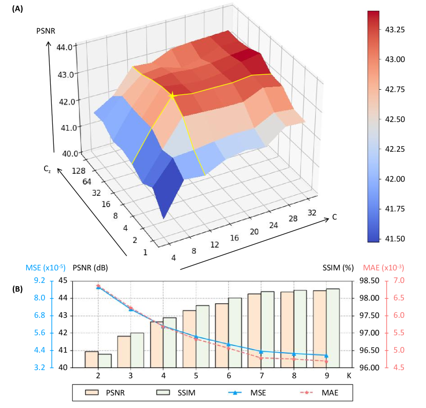
Figure 3: Experiment results on the influence of network parameters. (A) displays the 3D landscape of the reconstructed image PSNR, calculated from the parameter grid search about $C$ and $C_{z}$. The yellow star marks the choice of the optimal parameters, which correspond to $C=12$ and $C_{z}=8$. Experiment results on the influence of $K$ are shown in (B).

4.3 Evaluation Metrics

We used four quantitative metrics to provide a comprehensive evaluation of the reconstruction performance: mean square error (MSE), peak signal-to-noise ratio (PSNR), structural similarity index (SSIM), and mean absolute error (MAE):

$${\rm{MSE}} =\frac{1}{M}\left\|\hat{x}-x^{*}\right\|_{2}^{2},$$ (10)

$${\rm{PSNR}} =10{\rm{log}}_{10}\left(\frac{M}{\left\|\hat{x}-x^{*}\right\|_{2}^{2}}\right),$$

$${\rm{SSIM}} =\textbf{l}\left(\hat{x}-x^{*}\right)\cdot\textbf{c}\left(\hat{x}-x^{*}\right)\cdot\textbf{s}\left(\hat{x}-x^{*}\right),$$

$${\rm{MAE}} =\frac{1}{M}\left\|\hat{x}-x^{*}\right\|_{1}.$$

where $x^{*}$ is the ground-truth image and $\hat{x}$ is the reconstructed image, $M$ is the total number of image pixels. Details about the SSIM index are shown in [42]. The metrics are evaluated for each frame independently and then averaged to give the final value for the dynamic reconstruction. Besides, the unit for each metric is adjusted to ensure an appropriate value range: MSE ($\times 10^{-5}$), PSNR ($\rm{dB}$), SSIM ($\%$), MAE ($\times 10^{-3}$).

5 Experiments and Results

5.1 Effect of Algorithm Parameters

In this study, we investigated the influence of the algorithm hyper-parameters, which are divided into two categories:

5.1.1 Network Parameters

the parameters of $G_{\theta}$, including the network size parameter $C$, the latent variable channels $C_{z}$, and the number of neighbors $K$. Since a prohibitively long time is required to conduct a grid search over all parameter combinations, we empirically fixed the parameter $K$=5, and performed a grid search on $C$$\in${4,8,12,16,20,24,28,32} and $C_{z}$$\in${1,2,4,8,16,32,64,128}. After the optimal $C$ and $C_{z}$ are determined, we varied $K$$\in${2,3,4,5,6,7,8,9} to identify the best number of neighbors.

The results on the network parameters are shown in  Figure 3. We observed in  Figure 3(A) that when $C$ and $C_{z}$ are too small, the reconstruction performance is limited by the capacity of the generative model. The PSNR of the reconstructed image gradually increases with $C$ and $C_{z}$. This trend is approximately stopped at $C=12$ and $C_{z}=8$, after which the reconstruction performance seems to reach saturation, forming a plateau on the 3D landscape. Therefore, we set $(C,C_{z})=(12,8)$ as the best parameter. The results about $K$ are shown in  Figure 3(B). The reconstruction performance increases nearly monotonically with $K$. The turning point occurs at $K=7$, which is selected as the best value.

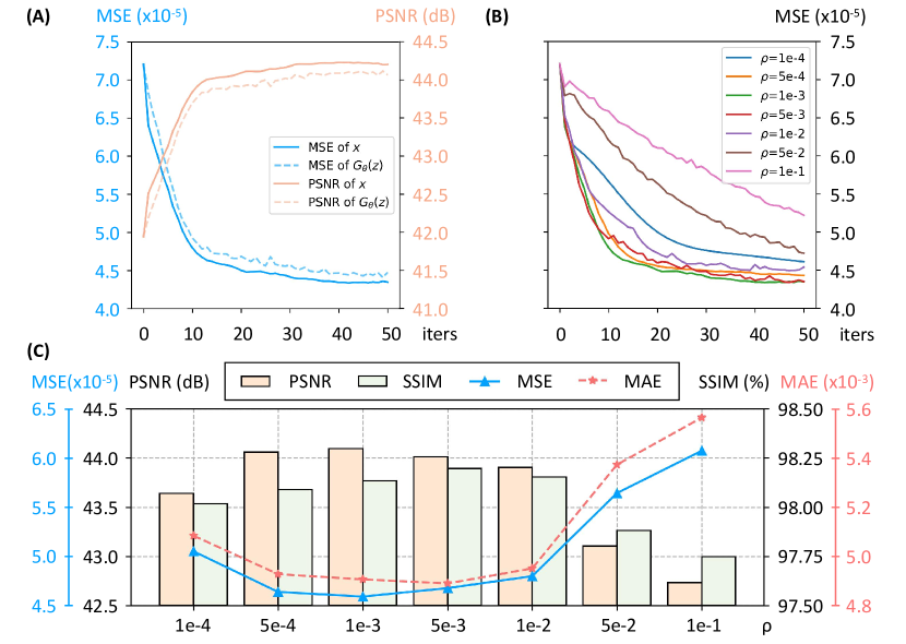
Figure 4: Experiment results on the influence of iteration parameters. (A) displays the MSE and PSNR curves related to the iteration steps, in which the reconstructed image $x$ is plotted by the solid line, and the generated image $G_{\theta}(z)$ is plotted by the dotted line. The MSE-iteration curves under different $\rho$ settings are shown in (B). The reconstruction performance under different $\rho$ settings are shown in (C).

5.1.2 ADMM Parameters

the parameters of the ADMM optimization algorithm. For each iteration, we used 10 CG steps and adopted the Adam optimizer with learning rate $lr$=$1\times 10^{-5}$ and $\beta$=$(0.5,0.98)$ to train the $G_{\theta}$ with 500 iterations. We mainly investigated the influence of two parameters: the number of ADMM iterations, and the relaxation parameter $\rho$. We varied $\rho$$\in${0.0001,0.0005,0.001,0.005,0.01,0.05,0.1}, and set the ADMM iterations to 50. The reconstructed images (including $G_{\theta}(z)$ and $x$) are evaluated for each $\rho$ and every iteration.

The results on the iteration parameters are shown in  Figure 4.  Figure 4(A) depicts the MSE and PSNR curves, which demonstrates that the ADMM algorithm comes to convergence as the iteration progresses. Besides, the image quality improvement of $x$ is closely accompanied by $G_{\theta}(z)$, indicating that the image $x$ and network parameters $\theta$ are indeed optimized simultaneously. The MSE curves under different $\rho$ settings are shown in (B). When $\rho$ is too large ($\rho$=0.1), the algorithm convergence will be significantly slowed down. When $\rho$ is too small ($\rho$=0.0001), the convergence also becomes slower, and the final solution seems to be worse. We fix the iterations to 20 and calculate the quantitative metrics under different $\rho$ values, as shown in (C), from which we select the best $\rho$=0.001.

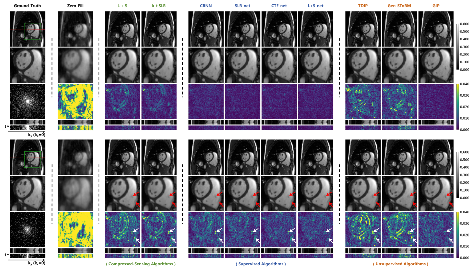
Figure 5: The reconstruction results of a case in the OCMR dataset. The upper half shows the results of R=8.0 and the lower half shows R=16.0. The first row displays, from left to right, the ground truth and the reconstructed images of different methods. The second row shows the zoomed-in image of the heart regions, framed by the green box on the ground-truth image. The third row shows the Poisson sampling mask and the reconstruction error maps for different methods. The fourth row shows the y-t motion profile (plotted at the red line in the ground truth image) and the corresponding error maps. The ky-t sampling pattern is plotted at the left-bottom corner. The grayscale range and error color bar are shown on the right side.

Table 1: Quantitative results on the OCMR dataset (Mean$\pm$Standard Deviation).

	Metrics	Compressed-Sensing		Supervised				Unsupervised
		L+S	k-t SLR	CRNN	SLR-net	CTF-net	L+S-net	TDIP	Gen-SToRM	GIP
R=8.0	MSE	2.25$\pm$1.10	2.21$\pm$0.92	1.18$\pm$0.70	0.95$\pm$0.54	0.83$\pm$0.48	0.75$\pm$0.43	4.63$\pm$2.35	6.64$\pm$3.47	0.98$\pm$0.45
	PSNR	47.30$\pm$2.57	47.15$\pm$2.09	50.27$\pm$3.01	51.11$\pm$2.85	51.82$\pm$3.06	52.14$\pm$2.92	44.76$\pm$2.57	42.73$\pm$2.44	50.63$\pm$2.08
	SSIM	99.22$\pm$0.32	99.30$\pm$0.28	99.58$\pm$0.24	99.63$\pm$0.21	99.68$\pm$0.18	99.70$\pm$0.18	98.68$\pm$0.49	98.08$\pm$0.83	99.59$\pm$0.18
	MAE	2.94$\pm$0.89	2.90$\pm$0.74	2.36$\pm$0.77	2.19$\pm$0.70	2.01$\pm$0.67	1.96$\pm$0.64	3.91$\pm$1.10	4.66$\pm$1.42	2.24$\pm$0.55
R=16.0	MSE	8.63$\pm$4.46	8.58$\pm$2.79	5.16$\pm$3.34	4.74$\pm$2.30	3.99$\pm$2.08	3.45$\pm$1.59	11.66$\pm$7.68	13.02$\pm$7.84	5.34$\pm$2.24
	PSNR	40.92$\pm$1.43	41.35$\pm$2.47	43.72$\pm$2.64	43.79$\pm$2.17	44.65$\pm$2.39	45.16$\pm$2.15	40.57$\pm$2.49	39.86$\pm$2.53	43.23$\pm$2.06
	SSIM	97.44$\pm$0.93	97.74$\pm$0.52	98.65$\pm$0.53	98.53$\pm$0.54	98.83$\pm$0.44	98.87$\pm$0.45	96.92$\pm$1.29	96.78$\pm$1.34	97.84$\pm$0.71
	MAE	6.11$\pm$1.19	5.88$\pm$1.66	4.77$\pm$1.56	4.64$\pm$1.24	4.24$\pm$1.23	4.02$\pm$1.05	6.27$\pm$1.76	6.28$\pm$1.94	5.33$\pm$1.23

5.2 Reconstruction Performance

The algorithms were adjusted to their best performance and evaluated on the OCMR dataset. 2D random Poisson masks are used for k-space sampling, which varies with different frames and the center region is fully sampled (ACS signals). Experiments were conducted under two acceleration settings (R=8.0, ACS=[10,10]) and (R=16.0, ACS=[6,6]).

The reconstructed images of a representative case are shown in  Figure 5. At R=8.0, L+S and k-t SLR can both produce good image quality. A relatively higher reconstructed error occurs at the blood-myocardium boundary. The supervised learning algorithms all achieve excellent reconstruction accuracy with very low error levels. For the unsupervised methods, TDIP and GenSToRM produce worse reconstruction quality, even compared with the CS methods. In comparison, the proposed GIP method achieves comparable reconstruction accuracy with the supervised methods, producing a uniform error map. At R=16.0, since fewer measurements are available, the reconstruction performances of all the algorithms decrease. Tiny structures are easily lost or blurred during reconstruction at such a high acceleration factor, especially for algorithms based on low-rank priors. However, as marked by the red arrows on the image and the white arrows on the error map, GIP achieves high reconstruction fidelity of the small details.

Table 2: Generalization results on the CMRxRecon dataset (Mean$\pm$Standard Deviation).

	Metrics	Compressed-Sensing		Supervised				Unsupervised
		L+S	k-t SLR	CRNN	SLR-net	CTF-net	L+S-net	TDIP	Gen-SToRM	GIP
R=8.0	MSE	2.26$\pm$2.10	2.11$\pm$1.71	1.75$\pm$1.62	1.26$\pm$0.62	1.08$\pm$0.66	1.43$\pm$2.28	5.73$\pm$2.74	10.06$\pm$7.35	0.87$\pm$0.34
	PSNR	47.15$\pm$2.03	47.35$\pm$1.92	48.34$\pm$2.23	49.43$\pm$1.83	50.21$\pm$1.98	49.67$\pm$2.51	43.05$\pm$1.83	40.86$\pm$2.40	50.90$\pm$1.62
	SSIM	99.06$\pm$0.25	99.18$\pm$0.18	99.31$\pm$0.25	99.41$\pm$0.18	99.50$\pm$0.16	99.46$\pm$0.20	97.82$\pm$0.56	96.36$\pm$1.99	99.53$\pm$0.13
	MAE	3.14$\pm$0.92	3.04$\pm$0.81	2.91$\pm$0.82	2.59$\pm$0.56	2.37$\pm$0.55	2.56$\pm$0.97	5.10$\pm$1.10	6.45$\pm$2.13	2.18$\pm$0.42
R=16.0	MSE	7.00$\pm$6.66	6.20$\pm$6.00	6.60$\pm$3.99	5.97$\pm$3.50	5.37$\pm$3.85	4.84$\pm$2.69	9.99$\pm$4.54	14.75$\pm$8.55	3.33$\pm$1.37
	PSNR	42.39$\pm$2.36	42.94$\pm$2.35	43.09$\pm$2.38	42.81$\pm$2.10	43.76$\pm$2.21	43.68$\pm$2.02	40.67$\pm$1.98	39.11$\pm$2.30	45.12$\pm$1.66
	SSIM	97.54$\pm$0.76	97.88$\pm$0.70	98.08$\pm$0.75	97.98$\pm$0.57	98.24$\pm$0.77	98.22$\pm$0.49	96.76$\pm$0.85	95.35$\pm$2.26	98.44$\pm$0.40
	MAE	5.34$\pm$1.71	4.91$\pm$1.56	5.14$\pm$2.02	5.16$\pm$1.24	4.73$\pm$1.64	4.73$\pm$1.10	6.34$\pm$1.36	7.52$\pm$2.21	4.21$\pm$0.84

Table 1 summarizes the quantitative results. We noticed that the supervised methods lead the first-level reconstruction performance at both acceleration settings, in which the L+S-net achieves the best results. The CS methods have a performance gap with the supervised methods, approximately 5dB in PSNR compared with the L+S-net method. The TDIP and Gen-SToRM methods display even worse performance compared with the CS methods. In comparison, the proposed GIP method significantly outperforms other CS and unsupervised methods, greatly reducing the gap with the supervised methods.

5.3 Generalization Performance

We compared the generalization ability of the reconstruction methods when they were transferred to a different dataset. We fixed the parameters adjusted in the OCMR dataset, and directly applied all the methods to reconstruct the CMRxRecon test set. 2D Poisson sampling with two acceleration settings (R=8.0, ACS=[12,12]) and (R=16.0, ACS=[8,8]) are evaluated.

Table 2 shows the quantitative results of the generalization experiment. The performance of the CS methods remains relatively stable when the dataset is changed. However, performance degradation occurs in all supervised algorithms, though most of them are still better than the CS methods. In comparison, GIP displays superior generalization performance, achieving the best score on all the quantitative metrics.

5.4 Ablation Experiments

We conducted ablation experiments to validate the effectiveness of the key components in the GIP method: the GCN network and the ADMM optimization algorithm. Specifically, we use “DIP only” to indicate that only the independent CNN generators $(G_{1},\ldots,G_{N})$ are used for reconstruction. “DIP+GCN” means utilizing the whole $G_{\theta}$ network for reconstruction by directly fitting the k-space data. “DIP+ADMM” means the CNN generators are used for reconstruction with the ADMM algorithm, in which the $G_{\theta}$ is substituted by $(G_{1},\ldots,G_{N})$. We also saved the intermediate results of different ADMM iterations to visualize the optimization process.

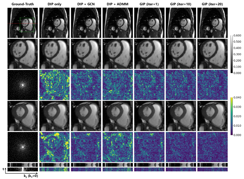
Figure 6: Illustration of the ablation study results. From left to right columns are the ground truth and the reconstruction results by “DIP only”, “DIP+GCN”, “DIP+ADMM’ and the proposed GIP method with 1, 10, and 20 iterations. The diastolic frames are displayed on the second row, and the third row displays the corresponding error maps. The results of the systolic frame are shown in the fourth and fifth row. The y-t motion profiles and error maps are shown at the bottom.

Table 3: Quantitative results of the ablation study.

	Metrics	DIP only	DIP + GCN	DIP + ADMM	GIP (iter=1)	GIP (iter=10)	GIP (iter=20)
R=8.0	MSE	23.91$\pm$8.15	2.59$\pm$0.96	5.67$\pm$1.62	1.44$\pm$0.62	1.17$\pm$0.50	0.98$\pm$0.45
	PSNR	36.52$\pm$1.36	46.23$\pm$1.70	42.69$\pm$1.27	48.93$\pm$2.01	49.83$\pm$1.97	50.63$\pm$2.08
	SSIM	94.20$\pm$0.98	99.05$\pm$0.34	97.64$\pm$0.40	99.40$\pm$0.23	99.51$\pm$0.19	99.59$\pm$0.18
	MAE	10.09$\pm$1.72	3.68$\pm$0.79	5.53$\pm$0.83	2.74$\pm$0.64	2.45$\pm$0.57	2.24$\pm$0.55
R=16.0	MSE	32.95$\pm$8.26	8.70$\pm$3.61	19.46$\pm$5.63	7.67$\pm$3.26	5.73$\pm$2.53	5.34$\pm$2.24
	PSNR	35.03$\pm$1.17	41.08$\pm$2.01	37.33$\pm$1.29	41.66$\pm$2.08	42.99$\pm$2.19	43.23$\pm$2.06
	SSIM	91.08$\pm$1.41	97.04$\pm$0.96	92.58$\pm$1.27	97.22$\pm$0.88	97.85$\pm$0.75	97.84$\pm$0.71
	MAE	12.27$\pm$1.78	6.64$\pm$1.56	10.14$\pm$1.52	6.24$\pm$1.48	5.42$\pm$1.34	5.33$\pm$1.23

The results of the ablation study are shown in  Figure 6. The “DIP only” approach can eliminate the undersampling artifacts to some extent; however, the reconstructed images exhibit significant blurring and artifacts. The “DIP+GCN” strategy utilizes the GCN to exploit the spatio-temporal correlations, significantly enhancing the reconstruction accuracy. The ”DIP+ADMM” method employs the ADMM optimization algorithm to leverage the structured priors of DIP, leading to improved reconstruction performance; however, its effectiveness is inferior to “DIP+GCN”. Our proposed GIP method synergistically incorporates DIP, GCN, and the ADMM optimizer into one algorithm, achieving the highest reconstruction fidelity.  Table 3 summarizes the quantitative results of the ablation study, corroborating the contribution of each component in GIP to the ultimate reconstruction performance.

5.5 Experiments on Other Sampling Trajectories

Because k-space trajectory needs to be continuous in a real MRI scan, the Poisson sampling mask could not be achieved for 2D MRI acquisition sequences. Therefore, we conducted reconstruction experiments using three physically feasible 2D sampling trajectories: Cartesian, Radial, and Spiral.

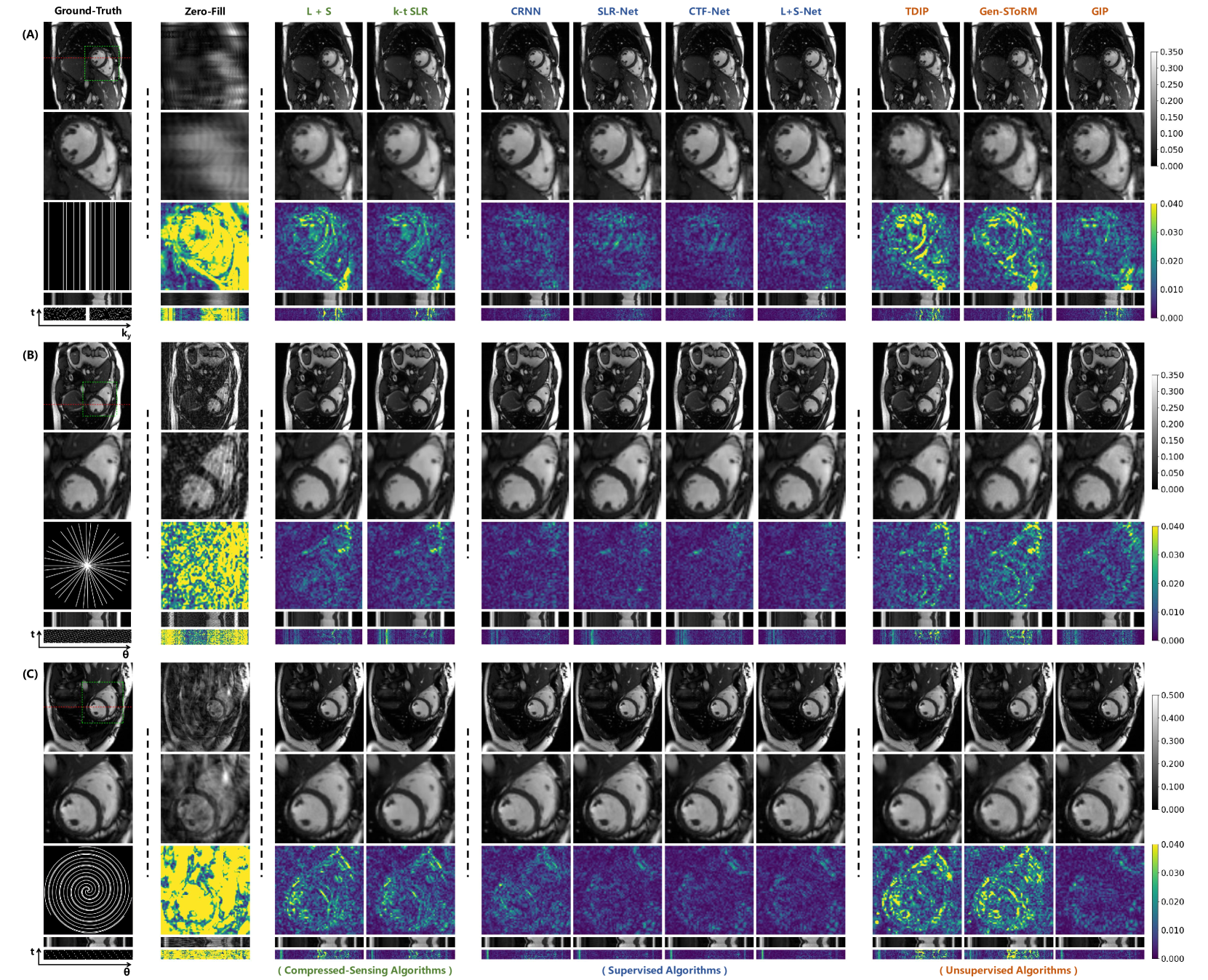
Figure 7: The reconstruction results of different k-space undersampling trajectories, where the Cartesian trajectory is shown in (A), Radial in (B) and Spiral in (C). For each trajectory, the first row displays the ground truth and the reconstructed images of different methods. The second row shows the zoomed-in image of the heart regions. The third row shows the sampling mask and the error maps. The fourth row shows the y-t motion profile and the corresponding error maps. The t-encoding sampling pattern is plotted at the left-bottom corner. The color bars are shown on the right side.

Table 4: Quantitative results of GIP vs. other methods on different sampling trajectories at acceleration factor R=8.0.

	Metrics	Compressed-Sensing		Supervised				Unsupervised
		L+S	k-t SLR	CRNN	SLR-net	CTF-net	L+S-net	TDIP	Gen-SToRM	GIP
Cartesian	MSE	12.87$\pm$7.12	10.25$\pm$5.33	5.18$\pm$2.65	4.51$\pm$2.38	3.98$\pm$2.15	3.70$\pm$2.05	20.29$\pm$15.50	19.77$\pm$12.47	8.93$\pm$5.42
	PSNR	39.73$\pm$2.47	40.70$\pm$2.46	43.57$\pm$2.23	44.21$\pm$2.32	44.80$\pm$2.44	45.18$\pm$2.59	38.49$\pm$2.72	38.08$\pm$2.57	41.62$\pm$2.95
	SSIM	96.57$\pm$1.39	97.16$\pm$1.01	98.51$\pm$0.53	98.60$\pm$0.51	98.78$\pm$0.49	98.85$\pm$0.51	95.61$\pm$2.06	95.29$\pm$2.30	97.67$\pm$1.04
	MAE	6.42$\pm$1.86	6.15$\pm$1.60	4.50$\pm$1.09	4.17$\pm$1.01	3.95$\pm$1.04	3.70$\pm$1.04	7.45$\pm$2.50	7.57$\pm$2.46	5.18$\pm$1.55
Radial	MSE	8.55$\pm$3.52	8.17$\pm$5.40	4.25$\pm$2.21	3.87$\pm$2.13	3.33$\pm$1.31	3.54$\pm$1.80	11.29$\pm$5.45	13.17$\pm$7.21	6.12$\pm$2.48
	PSNR	41.10$\pm$1.79	41.44$\pm$1.93	44.18$\pm$1.86	44.63$\pm$1.96	45.15$\pm$1.78	45.01$\pm$1.96	40.09$\pm$1.76	39.51$\pm$2.23	42.54$\pm$1.78
	SSIM	97.98$\pm$0.63	98.37$\pm$0.42	98.89$\pm$0.39	99.01$\pm$0.38	99.14$\pm$0.34	99.11$\pm$0.36	97.06$\pm$1.03	96.63$\pm$1.43	98.40$\pm$0.60
	MAE	5.70$\pm$1.41	5.60$\pm$1.77	4.30$\pm$1.10	4.03$\pm$1.12	3.77$\pm$0.90	3.85$\pm$1.05	6.54$\pm$1.56	6.85$\pm$1.83	5.14$\pm$1.16
Spiral	MSE	7.37$\pm$2.98	7.25$\pm$3.03	3.53$\pm$0.98	2.92$\pm$0.88	2.76$\pm$1.21	2.51$\pm$0.82	10.92$\pm$5.06	14.36$\pm$8.10	3.74$\pm$1.05
	PSNR	41.71$\pm$1.69	41.80$\pm$1.79	44.72$\pm$1.23	45.54$\pm$1.27	45.96$\pm$1.74	46.24$\pm$1.43	40.27$\pm$1.84	39.16$\pm$2.19	44.44$\pm$1.16
	SSIM	98.27$\pm$0.54	98.38$\pm$0.50	98.94$\pm$0.25	99.10$\pm$0.15	99.38$\pm$0.19	99.41$\pm$0.18	97.01$\pm$1.13	96.55$\pm$1.43	99.07$\pm$0.24
	MAE	5.23$\pm$1.22	5.26$\pm$1.32	3.98$\pm$0.69	3.67$\pm$0.65	3.40$\pm$0.80	3.25$\pm$0.69	6.40$\pm$1.43	7.02$\pm$1.93	4.00$\pm$0.73

For the Cartesian trajectory, the acceleration setting is R=8.0 and ACS=6. The ky encodings outside the ACS region are drawn from the uniform probability distribution. For the Radial trajectory, the acceleration factor is R=8.0, which corresponds to 18 spokes sampled for each frame. The spokes are 2-fold oversampled along the readout direction, and rotate according to the golden ratio angles $\bigtriangleup\theta\approx 111.246^{\circ}$[43]. For the Spiral trajectory, we use an equidistance Archimedean spiral trajectory, which has a readout length of $1002$ points and needs 32 interleaves to cover the k-space. The acceleration factor is R=8.0, leading to 4 interleaves acquired for each frame, which also rotate according to the golden angle interval.

For the non-Cartesian trajectories, the non-uniform fast Fourier Transform (NUFFT) is needed for image reconstruction. We re-implement all the algorithms in their non-uniform sampling version, in which the data consistency (DC) blocks and loss terms are all substituted by their NUFFT counterparts. An open-source library TorchKbNufft[44] is utilized to enable GPU acceleration and gradient back-propagation.

The experiment results on different trajectories are shown in  Figure 7, where the Cartesian trajectory is shown in (A), Radial in (B), and Spiral in (C). For the Cartesian trajectory, the reconstruction results of the CS methods are unsatisfactory, with noticeable blurring at the myocardium edges and over-smoothing in the y-t motion profiles. The supervised deep learning methods achieve significantly improved reconstruction performance, with good visual quality and clear image details. Among the unsupervised algorithms, the TDIP and Gen-SToRM methods showed relatively poor reconstruction performance, with evident image artifacts. In comparison, the GIP method displays better results than other CS and unsupervised methods. However, images reconstructed by GIP still exhibit higher local errors in the apex area, and the overall image quality still has a gap compared to the supervised methods. For the Radial trajectory, we noticed an improvement in the reconstruction performance of the CS and unsupervised methods. However, the CS and unsupervised methods still display higher errors in local image details. In contrast, the reconstruction performance of GIP is much closer to the supervised algorithms, with a quite uniform error map. The Spiral trajectory shows similar results as the Radial trajectory, in which the proposed GIP method could recover sharp image details and clear motion profiles, achieving comparable reconstruction quality to the supervised algorithms. The quantitative metrics are summarized in  Table 4. The GIP method outperforms the CS and other unsupervised algorithms on all trajectories. Besides, for the GIP method itself, we observed that the worst reconstruction results are obtained by the Cartesian trajectory. The Radial trajectory could produce better results, and the Spiral trajectory achieves the highest reconstruction accuracy among all the three trajectories.

6 Discussion

6.1 Analysis of the GIP Model

Previous studies have shown that the DIP generator structure is critical to its regularization effect[45]. In static image restoration, most works adopt a pyramid-shaped CNN generator and a Gaussian noise input[22][46], which is demonstrated to be asymptotically equivalent to a stationary Gaussian process prior[47]. However, dynamic images have a key distinction that there exist strong correlations between the frames. Existing methods for dynamic MRI reconstruction express the correlations as the proximity between the latent variables[24][25], using a single CNN to learn the direct mapping from the latent space topology to the dynamic image manifold. Besides, these methods have to utilize very low-dimensional latent variables to preserve the correlations in the latent space, further limiting the model’s capacity. In comparison, the GIP model employs a two-stage generative process that explicitly disentangles the structural prior of CNN and the spatiotemporal redundancies of dynamic data, improving the expression ability and reconstruction performance.

6.2 Benefit of the Alternated Optimization Algorithm

Despite the good regularization effect of DIP, CNN can also introduce a strong bias to the output images. It is well-known that images reconstructed by a pure CNN architecture tend to lose image texture and details[48]. For this reason, directly fitting the k-space often causes over-smoothing in the reconstructed images. Therefore, it is necessary to decouple image reconstruction from the constraints of the network structural prior. In this work, we devise an ADMM algorithm to alternately optimize network parameters and images, which allows us to update the images and priors synergistically, and control the contribution of the network’s output to the reconstruction results. Although the optimization objective is a non-convex problem, experimental results show that the optimization algorithm still has a good convergence property, and can significantly improve the reconstruction performance compared with directly fitting the k-space data.

6.3 The Sensitivity to Different Sampling Trajectories

In this work, four sampling trajectories are simulated for reconstruction: Poisson, Cartesian, Radial, and Spiral. The reconstruction performance of GIP demonstrated obvious sensitivity to the sampling trajectories. In fact, in the absence of a fully sampled dataset providing additional prior information, the behavior of the unsupervised methods is more similar to the CS methods rather than the supervised methods. An important conclusion in the compressed-sensing theory is the RIP condition[49], which states that sampling incoherence is an important prerequisite for effectively recovering a signal from sparse samples[50]. Although the RIP condition is derived for sparsity-based CS algorithms, we also noticed similar properties among the unsupervised methods, including TDIP, Gen-SToRM, and the GIP method. Experimental results show that both the CS and the unsupervised methods achieve the best results under the Poisson sampling trajectory and the worst under the Cartesian trajectory, with results of Radial and Spiral trajectories in between. Therefore, the proposed GIP method may be more suitable for reconstruction problems involving non-Cartesian trajectories, or 3D dynamic imaging applications that employ random sampling in the ky-kz plane.

6.4 Limitations and Future Directions

Although the proposed GIP method has shown promising results, it still has some limitations that need to be addressed in future research. The first is the long reconstruction time. Since the ADMM algorithm alternately optimizes the image and the network parameters, each iteration requires a separate network training. In this work, we fix the training iterations as 500, leading to a reconstruction time of about one hour for a single slice. Possible solutions may include exploring the optimal number of training iterations or designing accelerated optimization algorithms to shorten the reconstruction time. The second problem is the linear growth of the GIP model. Because GIP assigns an independent set of weights for each node, the model size and memory consumption are proportional to the number of frames. Therefore, GIP is mainly suitable for reconstruction problems with fewer frames, such as the gated dynamic MRI. For real-time dynamic imaging of a long period, the computational resource demand of the GIP model may become unacceptable. An interesting direction for future research could be designing a compromise model between the single-generator scheme and the GIP model, making a balance between resource consumption and model expression ability. Finally, this article mainly validates the GIP method in cardiac cine MRI reconstruction. Since the cine MRI data is relatively easy to obtain, supervised deep learning methods have an absolute advantage in terms of reconstruction accuracy and speed. However, in more challenging scenarios such as 4D blood flow imaging, it is very difficult to obtain high-quality training data. It is valuable to investigate the effectiveness of GIP in other dynamic imaging applications.

7 Conclusion

In this work, we proposed a new model for unsupervised dynamic MRI reconstruction named Graph Image Prior (GIP), which adopts a two-stage generative process. We utilized independent CNNs to recover the image structures and a graph convolutional network to exploit the spatiotemporal correlations. We also devised an ADMM algorithm to alternately optimize the images and network parameters to enhance the reconstruction accuracy. The proposed method outperforms other CS and unsupervised algorithms, and significantly reduces the performance gap with the state-of-art supervised deep-learning methods. Besides, GIP displays superior generalization performance without the need for any additional data.

References

- [1] J. Tsao, P. Boesiger, and K. P. Pruessmann, “k-t blast and k-t sense: dynamic mri with high frame rate exploiting spatiotemporal correlations,” Magnetic Resonance in Medicine: An Official Journal of the International Society for Magnetic Resonance in Medicine, vol. 50, no. 5, pp. 1031–1042, 2003.
- [2] Z.-P. Liang, “Spatiotemporal imagingwith partially separable functions,” in 2007 4th IEEE international symposium on biomedical imaging: from nano to macro. IEEE, 2007, pp. 988–991.
- [3] L. Feng, M. B. Srichai, R. P. Lim, A. Harrison, W. King, G. Adluru, E. V. Dibella, D. K. Sodickson, R. Otazo, and D. Kim, “Highly accelerated real-time cardiac cine mri using k–t sparse-sense,” Magnetic resonance in medicine, vol. 70, no. 1, pp. 64–74, 2013.
- [4] H. Jung, K. Sung, K. S. Nayak, E. Y. Kim, and J. C. Ye, “k-t focuss: a general compressed sensing framework for high resolution dynamic mri,” Magnetic Resonance in Medicine: An Official Journal of the International Society for Magnetic Resonance in Medicine, vol. 61, no. 1, pp. 103–116, 2009.
- [5] B. Zhao, J. P. Haldar, A. G. Christodoulou, and Z.-P. Liang, “Image reconstruction from highly undersampled (k, t)-space data with joint partial separability and sparsity constraints,” IEEE transactions on medical imaging, vol. 31, no. 9, pp. 1809–1820, 2012.
- [6] S. G. Lingala, Y. Hu, E. DiBella, and M. Jacob, “Accelerated dynamic mri exploiting sparsity and low-rank structure: kt slr,” IEEE transactions on medical imaging, vol. 30, no. 5, pp. 1042–1054, 2011.
- [7] R. Otazo, E. Candes, and D. K. Sodickson, “Low-rank plus sparse matrix decomposition for accelerated dynamic mri with separation of background and dynamic components,” Magnetic resonance in medicine, vol. 73, no. 3, pp. 1125–1136, 2015.
- [8] S. Poddar and M. Jacob, “Dynamic mri using smoothness regularization on manifolds (storm),” IEEE transactions on medical imaging, vol. 35, no. 4, pp. 1106–1115, 2015.
- [9] U. Nakarmi, Y. Wang, J. Lyu, D. Liang, and L. Ying, “A kernel-based low-rank (klr) model for low-dimensional manifold recovery in highly accelerated dynamic mri,” IEEE transactions on medical imaging, vol. 36, no. 11, pp. 2297–2307, 2017.
- [10] S. Wang, Z. Ke, H. Cheng, S. Jia, L. Ying, H. Zheng, and D. Liang, “Dimension: dynamic mr imaging with both k-space and spatial prior knowledge obtained via multi-supervised network training,” NMR in Biomedicine, vol. 35, no. 4, p. e4131, 2022.
- [11] Q. Huang, Y. Xian, D. Yang, H. Qu, J. Yi, P. Wu, and D. N. Metaxas, “Dynamic mri reconstruction with end-to-end motion-guided network,” Medical Image Analysis, vol. 68, p. 101901, 2021.
- [12] J. Sun, H. Li, Z. Xu et al., “Deep admm-net for compressive sensing mri,” Advances in neural information processing systems, vol. 29, 2016.
- [13] H. K. Aggarwal, M. P. Mani, and M. Jacob, “Modl: Model-based deep learning architecture for inverse problems,” IEEE transactions on medical imaging, vol. 38, no. 2, pp. 394–405, 2018.
- [14] K. Hammernik, T. Klatzer, E. Kobler, M. P. Recht, D. K. Sodickson, T. Pock, and F. Knoll, “Learning a variational network for reconstruction of accelerated mri data,” Magnetic resonance in medicine, vol. 79, no. 6, pp. 3055–3071, 2018.
- [15] J. Schlemper, J. Caballero, J. V. Hajnal, A. N. Price, and D. Rueckert, “A deep cascade of convolutional neural networks for dynamic mr image reconstruction,” IEEE transactions on Medical Imaging, vol. 37, no. 2, pp. 491–503, 2017.
- [16] C. Qin, J. Schlemper, J. Caballero, A. N. Price, J. V. Hajnal, and D. Rueckert, “Convolutional recurrent neural networks for dynamic mr image reconstruction,” IEEE transactions on medical imaging, vol. 38, no. 1, pp. 280–290, 2018.
- [17] C. Qin, J. Duan, K. Hammernik, J. Schlemper, T. Küstner, R. Botnar, C. Prieto, A. N. Price, J. V. Hajnal, and D. Rueckert, “Complementary time-frequency domain networks for dynamic parallel mr image reconstruction,” Magnetic Resonance in Medicine, vol. 86, no. 6, pp. 3274–3291, 2021.
- [18] J. Zhang and B. Ghanem, “Ista-net: Interpretable optimization-inspired deep network for image compressive sensing,” in Proceedings of the IEEE conference on computer vision and pattern recognition, 2018, pp. 1828–1837.
- [19] Z. Ke, W. Huang, Z.-X. Cui, J. Cheng, S. Jia, H. Wang, X. Liu, H. Zheng, L. Ying, Y. Zhu et al., “Learned low-rank priors in dynamic mr imaging,” IEEE Transactions on Medical Imaging, vol. 40, no. 12, pp. 3698–3710, 2021.
- [20] W. Huang, Z. Ke, Z.-X. Cui, J. Cheng, Z. Qiu, S. Jia, L. Ying, Y. Zhu, and D. Liang, “Deep low-rank plus sparse network for dynamic mr imaging,” Medical Image Analysis, vol. 73, p. 102190, 2021.
- [21] D. Ulyanov, A. Vedaldi, and V. Lempitsky, “Deep image prior,” in Proceedings of the IEEE conference on computer vision and pattern recognition, 2018, pp. 9446–9454.
- [22] M. Z. Darestani and R. Heckel, “Accelerated mri with un-trained neural networks,” IEEE Transactions on Computational Imaging, vol. 7, pp. 724–733, 2021.
- [23] K. Gong, C. Catana, J. Qi, and Q. Li, “Pet image reconstruction using deep image prior,” IEEE transactions on medical imaging, vol. 38, no. 7, pp. 1655–1665, 2018.
- [24] J. Yoo, K. H. Jin, H. Gupta, J. Yerly, M. Stuber, and M. Unser, “Time-dependent deep image prior for dynamic mri,” IEEE Transactions on Medical Imaging, vol. 40, no. 12, pp. 3337–3348, 2021.
- [25] Q. Zou, A. H. Ahmed, P. Nagpal, S. Kruger, and M. Jacob, “Dynamic imaging using a deep generative storm (gen-storm) model,” IEEE transactions on medical imaging, vol. 40, no. 11, pp. 3102–3112, 2021.
- [26] A. H. Ahmed, Q. Zou, P. Nagpal, and M. Jacob, “Dynamic imaging using deep bi-linear unsupervised representation (deblur),” IEEE transactions on medical imaging, vol. 41, no. 10, pp. 2693–2703, 2022.
- [27] Y. Q. Mohsin, S. Poddar, and M. Jacob, “Free-breathing & ungated cardiac mri using iterative storm (i-storm),” IEEE transactions on medical imaging, vol. 38, no. 10, pp. 2303–2313, 2019.
- [28] S. Poddar, Y. Q. Mohsin, D. Ansah, B. Thattaliyath, R. Ashwath, and M. Jacob, “Manifold recovery using kernel low-rank regularization: Application to dynamic imaging,” IEEE transactions on computational imaging, vol. 5, no. 3, pp. 478–491, 2019.
- [29] U. Nakarmi, K. Slavakis, and L. Ying, “Mls: Joint manifold-learning and sparsity-aware framework for highly accelerated dynamic magnetic resonance imaging,” in 2018 IEEE 15th International Symposium on Biomedical Imaging (ISBI 2018). IEEE, 2018, pp. 1213–1216.
- [30] Z. Wu, S. Pan, F. Chen, G. Long, C. Zhang, and S. Y. Philip, “A comprehensive survey on graph neural networks,” IEEE transactions on neural networks and learning systems, vol. 32, no. 1, pp. 4–24, 2020.
- [31] A. Sandryhaila and J. M. Moura, “Discrete signal processing on graphs,” IEEE transactions on signal processing, vol. 61, no. 7, pp. 1644–1656, 2013.
- [32] M. Defferrard, X. Bresson, and P. Vandergheynst, “Convolutional neural networks on graphs with fast localized spectral filtering,” Advances in neural information processing systems, vol. 29, 2016.
- [33] T. N. Kipf and M. Welling, “Semi-supervised classification with graph convolutional networks,” arXiv preprint arXiv:1609.02907, 2016.
- [34] G. Li, M. Muller, A. Thabet, and B. Ghanem, “Deepgcns: Can gcns go as deep as cnns?” in Proceedings of the IEEE/CVF international conference on computer vision, 2019, pp. 9267–9276.
- [35] K. Han, Y. Wang, J. Guo, Y. Tang, and E. Wu, “Vision gnn: An image is worth graph of nodes,” Advances in Neural Information Processing Systems, vol. 35, pp. 8291–8303, 2022.
- [36] F. Cheng, Y. Liu, Y. Chen, and P.-T. Yap, “High-resolution 3d magnetic resonance fingerprinting with a graph convolutional network,” IEEE transactions on medical imaging, vol. 42, no. 3, pp. 674–683, 2022.
- [37] H. Lu, H. Ye, L. L. Wald, and B. Zhao, “Accelerated mr fingerprinting with low-rank and generative subspace modeling,” arXiv preprint arXiv:2305.10651, 2023.
- [38] C. Chen, Y. Liu, P. Schniter, M. Tong, K. Zareba, O. Simonetti, L. Potter, and R. Ahmad, “Ocmr (v1. 0)–open-access multi-coil k-space dataset for cardiovascular magnetic resonance imaging,” arXiv preprint arXiv:2008.03410, 2020.
- [39] T. Zhang, J. M. Pauly, S. S. Vasanawala, and M. Lustig, “Coil compression for accelerated imaging with cartesian sampling,” Magnetic resonance in medicine, vol. 69, no. 2, pp. 571–582, 2013.
- [40] C. Wang, J. Lyu, S. Wang, C. Qin, K. Guo, X. Zhang, X. Yu, Y. Li, F. Wang, J. Jin et al., “Cmrxrecon: an open cardiac mri dataset for the competition of accelerated image reconstruction,” arXiv preprint arXiv:2309.10836, 2023.
- [41] M. Uecker, P. Lai, M. J. Murphy, P. Virtue, M. Elad, J. M. Pauly, S. S. Vasanawala, and M. Lustig, “Espirit—an eigenvalue approach to autocalibrating parallel mri: where sense meets grappa,” Magnetic resonance in medicine, vol. 71, no. 3, pp. 990–1001, 2014.
- [42] Z. Wang, A. C. Bovik, H. R. Sheikh, and E. P. Simoncelli, “Image quality assessment: from error visibility to structural similarity,” IEEE transactions on image processing, vol. 13, no. 4, pp. 600–612, 2004.
- [43] S. Winkelmann, T. Schaeffter, T. Koehler, H. Eggers, and O. Doessel, “An optimal radial profile order based on the golden ratio for time-resolved mri,” IEEE transactions on medical imaging, vol. 26, no. 1, pp. 68–76, 2006.
- [44] M. J. Muckley, R. Stern, T. Murrell, and F. Knoll, “TorchKbNufft: A high-level, hardware-agnostic non-uniform fast Fourier transform,” in ISMRM Workshop on Data Sampling & Image Reconstruction, 2020, source code available at https://github.com/mmuckley/torchkbnufft.
- [45] M. E. Arican, O. Kara, G. Bredell, and E. Konukoglu, “Isnas-dip: Image-specific neural architecture search for deep image prior,” in Proceedings of the IEEE/CVF Conference on Computer Vision and Pattern Recognition, 2022, pp. 1960–1968.
- [46] R. Heckel and P. Hand, “Deep decoder: Concise image representations from untrained non-convolutional networks,” arXiv preprint arXiv:1810.03982, 2018.
- [47] Z. Cheng, M. Gadelha, S. Maji, and D. Sheldon, “A bayesian perspective on the deep image prior,” in Proceedings of the IEEE/CVF Conference on Computer Vision and Pattern Recognition, 2019, pp. 5443–5451.
- [48] G. Yang, S. Yu, H. Dong, G. Slabaugh, P. L. Dragotti, X. Ye, F. Liu, S. Arridge, J. Keegan, Y. Guo et al., “Dagan: Deep de-aliasing generative adversarial networks for fast compressed sensing mri reconstruction,” IEEE transactions on medical imaging, vol. 37, no. 6, pp. 1310–1321, 2017.
- [49] R. G. Baraniuk, “Compressive sensing [lecture notes],” IEEE signal processing magazine, vol. 24, no. 4, pp. 118–121, 2007.
- [50] M. Lustig, D. Donoho, and J. M. Pauly, “Sparse mri: The application of compressed sensing for rapid mr imaging,” Magnetic Resonance in Medicine: An Official Journal of the International Society for Magnetic Resonance in Medicine, vol. 58, no. 6, pp. 1182–1195, 2007.