FusionINN: Invertible Image Fusion for Brain Tumor Monitoring

Abstract

Image fusion typically employs non-invertible neural networks to merge multiple source images into a single fused image. However, for clinical experts, solely relying on fused images may be insufficient for making diagnostic decisions, as the fusion mechanism blends features from source images, thereby making it difficult to interpret the underlying tumor pathology. We introduce FusionINN, a novel invertible image fusion framework, capable of efficiently generating fused images and also decomposing them back to the source images by solving the inverse of the fusion process. FusionINN guarantees lossless one-to-one pixel mapping by integrating a normally distributed latent image alongside the fused image to facilitate the generative modeling of the decomposition process. To the best of our knowledge, we are the first to investigate the decomposability of fused images, which is particularly crucial for life-sensitive applications such as medical image fusion compared to other tasks like multi-focus or multi-exposure image fusion. Our extensive experimentation validates FusionINN over existing discriminative and generative fusion methods, both subjectively and objectively. Moreover, compared to a recent denoising diffusion-based fusion model, our approach offers faster and qualitatively better fusion results. We also exhibit the clinical utility of our results in aiding disease prognosis.

1 Introduction

Magnetic Resonance Imaging (MRI) techniques, such as Diffusion-weighted imaging with Apparent Diffusion Coefficient (DWI-ADC) and T2-weighted Fluid Attenuated Inversion Recovery (T2-Flair), offer invaluable insights into the intricate pathology of tumors. A high-intensity signal on the T2-Flair image provides anatomical information about the presence of tumor and its boundary [1]. In contrast, DWI-ADC assist in revealing the tumor category, as a high-intensity signal indicates the existence of liquid components, i.e., necrotic tumor tissues and a low-intensity signal suggests the presence of solid components, i.e. enhancing tumor tissues [2]. Clinicians commonly utilize such image modalities post-operatively to detect any residual necrotic tumor tissues and assess the potential for its recurrence by locating enhancing tumor tissues. Fused images can aid in the visualization of the clinical features from multiple sources. However, merging grayscale values can obscure salient features, thereby complicating clinical interpretation of the fused image. To address this problem, we introduce the extended fusion task illustrated in Fig. 1, which demands decomposability of the fused image into the source images.

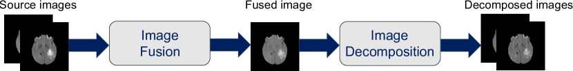
Figure 1: An illustration of the task of image fusion and decomposition.

Prior works in image fusion leverage deep learning algorithms via discriminative training [3, 4, 5, 6, 7, 10] or generative modeling using generative adversarial networks (GANs) [8]. However, the network architecture of such image fusion approaches is not invertible. Recently, a pre-trained Denoising Diffusion based image fusion model [9] has been proposed, that conditions each of the denoising diffusion steps on source images. In principle, diffusion models allow stable training dynamics, while not suffering from mode collapse. However, the decomposability of the fused images is not feasible using [9] as the pre-trained UNet [17] model used to perform the denoising steps is not invertible. Additionally, diffusion models perform slow sequential sampling through multiple denoising steps to obtain the fusion output, making real-time inference scheme infeasible.

We present normalizing flows as the generative model for medical image fusion and capitalize on their inherent invertibility to facilitate the decomposability of the fusion process. The flow also exhibits efficient sampling capabilities and stability during training using simple and invertible transformations. Previous attempts utilizing invertible neural networks (INNs) for image fusion [11, 12, 13, 14, 15] have predominantly integrated INNs only as a sub-module within a multi-step pipeline, preventing the invertibility of the end-to-end fusion procedure. Notably, no prior work has proposed image fusion as an inverse problem, modeled via an end-to-end INN that performs both image fusion and decomposition mechanisms. Our primary contributions include:

• We introduce a first-of-its-kind image fusion framework, FusionINN, that harnesses invertible normalizing flow for bidirectional training. FusionINN not only generates a fused image but can also decompose it into constituent source images, thus enhancing the interpretability for clinical practitioners.

• We present an extensive evaluation study that shows state-of-the-art results of FusionINN with common fusion metrics, alongside its additional capability to decompose the fused images.

• We illustrate FusionINN’s clinical viability by effectively decomposing and fusing new images from source modalities not encountered during training. Therefore, the model assists clinicians in accurately delineating tumor boundaries and visualizing tumor categories within those boundaries.

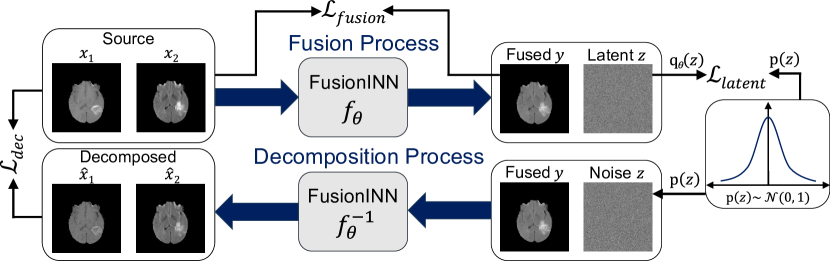
Figure 2: An overview of the FusionINN framework.

2 Method

The objective under decomposable image fusion, as depicted in Fig. 1, is to generate a fused image that closely resembles the source images and can be decomposed back into those source images without additional information.

2.1 INN-based Decomposable Image Fusion

The FusionINN framework for decomposable image fusion is shown in Fig. 2. In the forward fusion process, the FusionINN transforms the two source images $x_{1}\in\mathbb{R}^{n}$ and $x_{2}\in\mathbb{R}^{n}$ to the fused image $y\in\mathbb{R}^{n}$ and the latent image $z\in\mathbb{R}^{n}$ using the normalizing flow network $f$ with parameters $\theta$ such that $[y,z]=f_{\theta}(x_{1},x_{2})$, where $n$ is the number of pixels in the four equal resolution images. We add a latent image $z$ to the framework since the forward mapping from two source images into just one fused image, i.e., $f_{\theta}:\mathbb{R}^{2n}\rightarrow\mathbb{R}^{n}$ is an ill-posed inverse problem, thereby preventing the fusion model from being invertible. We formulate the latent image $z$ to follow a multivariate normal distribution such that $z\sim p(z)=\mathcal{N}(z;0,I)$ and the dimensionality of $[y,z]$ matches $[x_{1},x_{2}]$ with $f_{\theta},f^{-1}_{\theta}:\mathbb{R}^{2n}\leftrightarrow\mathbb{R}^{2n}$. Finally, the decomposition process is performed by using a newly sampled latent image $z$, along with the fused image $y$ through the reverse direction of FusionINN i.e. $f_{\theta}^{-1}$ to produce the decomposed images $\hat{x}_{1}$ and $\hat{x}_{2}$, such that $[\hat{x}_{1},\hat{x}_{2}]=f^{-1}_{\theta}([y,z])$. The inverse of the FusionINN i.e. $f_{\theta}^{-1}$ should aim to decompose the fused image $y$, independent from the latent image $z$.

2.2 INN Architecture

The FusionINN as a normalizing flow network $f_{\theta}$ consists of $k$ invertible coupling blocks stacked together such that $f=f_{k}\circ...f_{j}\circ...f_{1}$ with $[\hat{x}_{1},\hat{x}_{2}]=f_{\theta}^{-1}(y,z)$ and $[y,z]=f_{\theta}(x_{1},x_{2})$. In [20], the coupling blocks consists of transformations, scaling $s$ and translation $t$, which we construct as two convolutional layers with ReLU activation after each layer. The input to an arbitrary $j^{th}$ coupling block is first split into two parts $u^{j}_{1}$ and $u^{j}_{2}$, which are transformed by $s_{1},t_{1}$ and $s_{2},t_{2}$ networks that share the learnable parameters. The output of the $j^{th}$ coupling block is the concatenation of the resulting parts $v^{j}_{1}$ and $v^{j}_{2}$ given as:

$$v^{j}_{1}=u^{j}_{1}\odot\exp\big{(}s_{2}(u^{j}_{2})\big{)}+t_{2}(u^{j}_{2}),\ \ \ \\ v^{j}_{2}=u^{j}_{2}\odot\exp\big{(}s_{1}(v^{j}_{1})\big{)}+t_{1}(v^{j}_{1})$$ (1)

where $\odot$ is the element-wise multiplication, and the exponential term ensures non-zero coefficients. By construction, such a transformation is invertible, and $u^{j}_{1},u^{j}_{2}$ can be recovered from $v^{j}_{1},v^{j}_{2}$ (see [27]). After each coupling block, we implement a random permutation to reorganize the two channels corresponding to the source image modalities. This approach ensures that all channels contribute to influencing FusionINN’s learnable parameters, $\theta$.

2.3 Unsupervised Learning

The learning scheme of our framework is shown in Fig. 2. As there is no pre-defined fusion groundtruth, we formulate the fusion task in the forward process as a fully unsupervised problem with the fusion loss $\mathcal{L}_{fusion}$. FusionINN also learns to guide the latent image $z$ to follow standard normal distribution using $\mathcal{L}_{latent}$ loss. In the reverse process, the decomposition loss is defined as $\mathcal{L}_{dec}$.

2.3.1 Fusion Loss:

To learn the fused image $y$ from the flow network $f_{\theta}$ in an unsupervised manner, we follow [3] and leverage the metric Structural Similarity Index ($Q_{SSIM}$) [21] as the differentiable loss function to maximize the similarity between the source and the fused images. The loss function is formulated as:

$$\begin{gathered}\mathcal{L}_{SSIM}=\{1-Q_{SSIM}(x_{1},y)\}+\{1-Q_{SSIM}(x_{2},y)\}\end{gathered}$$ (2)

The sub-loss terms in $\mathcal{L}_{SSIM}$ are subtracted from 1 to satisfy the loss minimization objective, as the $Q_{SSIM}$ function inherently maximizes the similarity between the images. Moreover, it allows for brightness artifacts in the fused image, as discussed in [25]. Therefore, we use the $\ell_{2}$-loss in addition to the $Q_{SSIM}$ metric to better preserve the luminance of the fused image. Finally, given the weightage parameter as $\lambda$, the $\mathcal{L}_{\ell_{2}}$ and $\mathcal{L}_{fusion}$ losses are expressed as:

$$\begin{gathered}\mathcal{L}_{\ell_{2}}=||y-x_{1}||_{2}+||y-x_{2}||_{2},\ \ \ \mathcal{L}_{fusion}=\{\lambda*\mathcal{L}_{SSIM}+(1-\lambda)*\mathcal{L}_{\ell_{2}}\}\end{gathered}$$ (3)

2.3.2 Latent Loss:

We model the distribution of the latent image $z$ with a multivariate Gaussian $p(z)=\mathcal{N}(z;0,I)$. We utilize Maximum Mean Discrepancy ($\mathrm{MMD}$) [26] as the loss function to quantify the difference between the probability distribution $p(z)$ and the distribution $q_{\theta}(z)$ of the latent image $z$ generated by the forward process of the FusionINN model, $f_{\theta}$. Consequently, the latent loss $\mathcal{L}_{latent}$ is defined as $\mathcal{L}_{latent}=\mathrm{MMD}(q_{\theta}(z)\|p(z))$. Unlike the fused image $y$, which is normalized using the sigmoid function before applying the $\mathcal{L}_{fusion}$ loss, we do not impose such constraints on the latent image $z$ predicted by the FusionINN model, $f_{\theta}$. This enables the distribution $q_{\theta}(z)$ to approximate the standard normal distribution $p(z)$ after minimization of the $\mathcal{L}_{latent}$ loss.

2.3.3 Decomposition Loss:

We define the decomposition loss $\mathcal{L}_{dec}$ in the reverse direction of $f_{\theta}$ i.e. $f^{-1}_{\theta}$ to decompose the fused image $y$ back to the source images, using a newly sampled latent image $z$. We implement the $\mathcal{L}_{dec}$ loss as the combination of the $\mathcal{L}^{SSIM}_{dec}$ and $\mathcal{L}^{\ell_{2}}_{dec}$ losses, which are weighted using the meta-parameter $\lambda$, similar to the $\mathcal{L}_{fusion}$ loss. The $\mathcal{L}^{SSIM}_{dec}$ loss employs the $Q_{SSIM}$ metric to measure the similarity between the decomposed and the source images, while $\mathcal{L}^{\ell_{2}}_{dec}$ computes the $\ell_{2}$-loss between them. Hence, given the decomposed images $\hat{x}_{1}$ and $\hat{x}_{2}$, the losses $\mathcal{L}^{SSIM}_{dec}$, $\mathcal{L}^{\ell_{2}}_{dec}$ and $\mathcal{L}_{dec}$ are given as:

$$\begin{gathered}\mathcal{L}^{SSIM}_{dec}=\{1-Q_{SSIM}(x_{1},\hat{x}_{1})\}+\{1-Q_{SSIM}(x_{2},\hat{x}_{2})\}\\ \mathcal{L}^{\ell_{2}}_{dec}=||\hat{x}_{1}-x_{1}||_{2}+||\hat{x}_{2}-x_{2}||_{2},\ \ \ \mathcal{L}_{dec}=\lambda*\mathcal{L}^{SSIM}_{dec}+(1-\lambda)*\mathcal{L}^{\ell_{2}}_{dec}\end{gathered}$$ (4)

2.3.4 Training Procedure and Total Loss:

In the forward training process, the FusionINN optimizes the mapping $[y,z]=f_{\theta}(x_{1},x_{2})$ using $\mathcal{L}_{fusion}$ and $\mathcal{L}_{latent}$ losses. In the reverse training process, a new latent image $z$ is sampled from the normal distribution $p(z)$ to ensure the independence of the decomposition task from any specific $z$. Additionally, FusionINN’s invertibility guarantees that the latent image generated from the forward fusion process precisely reproduces the source images. Therefore, sampling a new latent image is necessary to assess the decomposition performance accurately. Hence, the resampled latent image $z$, together with the fused image $y$ is used to solve the reverse process by optimizing the mapping $[\hat{x}_{1},\hat{x}_{2}]=f^{-1}_{\theta}(y,z)$ using the $\mathcal{L}_{dec}$ loss. Finally, we weight the forward losses i.e., $\mathcal{L}_{fusion}$ and $\mathcal{L}_{latent}$ as well as the decomposition loss i.e., $\mathcal{L}_{dec}$ using the parameter $\alpha$ and formulate the total loss function $\mathcal{L}_{total}$ as follows:

$$\begin{gathered}\mathcal{L}_{total}=\{\alpha*(\mathcal{L}_{fusion}+\mathcal{L}_{latent})+(1-\alpha)*\mathcal{L}_{dec}\}\\ \end{gathered}$$ (5)

3 Results and Discussion

3.0.1 Data Description:

We use the publicly available BraTS-2018 brain imaging dataset [29] to prepare our training and validation data. We extract post-contrast T1-weighted (T1-Gd) and T2-Flair as the two source images, acquired with different clinical protocols and different scanners from multiple medical institutions. The data has been pre-processed, i.e., co-registered to the same anatomical template, interpolated to the same resolution and skull-stripped [29]. We only extract those images from the dataset where the clinical annotation comprises of the necrotic core, non-enhancing tumor, and the peritumoral edema. This results in 9653 image pairs of T1-Gd and T2-Flair modalities. We randomly assign 8500 image pairs as training and 1153 image pairs as the validation set.

Table 1: Comparison of the fusion performance of the evaluated models on the validation set of our pre-processed BraTS-2018 images [29]. The results from each model show averaged scores from five metrics after comparing the fused images with the source image pairs. For each metric, the best-performing model is highlighted in bold.

Model Type	Model Name	$Q_{SSIM}$ $\uparrow$	$Q_{FMI}$ $\uparrow$	$Q_{NCIE}$ $\uparrow$	$Q_{XY}$ $\uparrow$	$Q_{P}$ $\uparrow$
Discriminative	DeepFuse [3]	$0.927$	$0.791$	$0.806$	$0.449$	$0.766$
(Equal Dimension)	FunFuseAn [5]	$0.930$	$0.845$	$0.806$	$0.481$	$0.781$
Discriminative	Half-UNet [16]	$0.933$	$0.850$	$0.805$	$0.464$	$0.774$
(Dimension Reduction)	UNet [17]	$0.934$	$0.835$	$0.805$	$0.420$	$0.711$
	UNet++ [18]	$\mathbf{0.937}$	$0.849$	$0.805$	$0.433$	$0.739$
	UNet3+ [19]	$0.937$	$0.849$	$0.805$	$0.434$	$0.742$
Generative	DDFM [9]	$0.921$	$\mathbf{0.861}$	$0.806$	$0.472$	$0.702$
	FusionINN (Ours)	$0.927$	$0.835$	$\mathbf{0.806}$	$\mathbf{0.493}$	$\mathbf{0.783}$

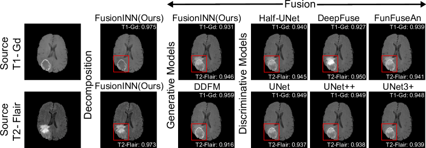
Figure 3: Fusion results obtained from the evaluated models on a sample validation image pair. The $Q_{SSIM}$ scores for individual modalities are shown in the fused images.

3.0.2 Competitive Methods and Evaluation Metrics:

We assess FusionINN’s performance by comparing it with other fusion methods, namely DeepFuse [3] and FunFuseAn [5]. We also repurpose popular image segmentation models namely Half-UNet [16], UNet [17], UNet++ [18], and UNet3+[19] for the image fusion task. Each of these models involve discriminative modeling and are trained on the fusion loss, i.e., $\mathcal{L}_{fusion}$ (Eq. 3). These models are non-invertible during training and only predict fused images. We maintain a common benchmark of meta-parameters during training of these models. Furthermore, we employ the pre-trained Denoising Diffusion-based Fusion model (DDFM) [9] as a generative method to evaluate its performance on our validation images. We utilize five quantitative metrics specifically designed for assessing the image fusion quality. The metrics are Feature Mutual Information ($Q_{FMI}$) [28], Structural Similarity Index ($Q_{SSIM}$) [21], Non-linear Correlation Information Entropy ($Q_{NCIE}$) [24], and by Petrovic et al. ($Q_{XY}$) [22], and Piella et al. ($Q_{P}$) [23]. The metric $Q_{XY}$ use gradient representation of the input images to quantify the information or feature transfer to the fused images. On the other hand, $Q_{P}$ weight the structural similarity scores based on local saliencies of the two input images.

Table 2: The effect of coupling blocks $k$, latent image $z$, and parameters $\lambda,\alpha$ on the fusion and decomposition performance. The results are averaged $Q_{SSIM}$ scores over the validation images with $Q_{SSIM}(x,y)$ for fusion and $Q_{SSIM}(x,\hat{x})$ for decomposition. For studying $\alpha,\lambda$ and $k$, we fix $z\sim\mathcal{N}(z;0,I)$. We fix $k=3$ for studying latent image $z$.

Weight ($\alpha$)	Fusion		Decomposition
($k=3,\lambda=0.8$)	T1-Gd	T2-Flair	T1-Gd	T2-Flair
0.2	0.903	0.929	0.930	0.930
0.5	0.921	0.933	0.976	0.972
0.8	0.926	0.933	0.927	0.920
1.0	0.948	0.898	0.033	0.004

Weight ($\lambda$)	Fusion		Decomposition
($k=3,\alpha=0.5$)	T1-Gd	T2-Flair	T1-Gd	T2-Flair
0.8	0.921	0.933	0.976	0.972
0.9	0.925	0.929	0.974	0.974
0.99	0.915	0.928	0.969	0.974
0.999	0.935	0.923	0.937	0.920

Blocks ($k$)	Fusion		Decomposition
($\alpha=0.5,\lambda=0.8$)	T1-Gd	T2-Flair	T1-Gd	T2-Flair
1	0.914	0.943	0.151	0.093
2	0.935	0.923	0.945	0.928
3	0.921	0.933	0.976	0.972
4	0.923	0.936	0.937	0.939

Latent ($z$)	Fusion		Decomposition
($\alpha=0.5,\lambda=0.8$)	T1-Gd	T2-Flair	T1-Gd	T2-Flair
0	0.918	0.930	0.932	0.928
$\mathcal{N}(0,I)$	0.921	0.933	0.976	0.972
$\mathcal{U}[0,I)$	0.924	0.925	0.958	0.954
1	0.916	0.929	0.967	0.969

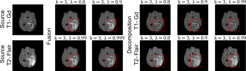
Figure 4: Qualitative results of our FusionINN model at $\alpha=0.5$ and $z\sim\mathcal{N}(0,I)$.

3.0.3 Fusion and Decomposition Performance:

Table 1 presents the quantitative fusion results of the evaluated models across various metrics after averaging over the validation images. Our FusionINN model demonstrates comparable or superior fusion performance with respect to all other evaluated methods across metrics such as $Q_{NCIE}$, $Q_{XY}$, and $Q_{P}$. Notably, FusionINN also exhibits competitive results on $Q_{SSIM}$ metric. Moreover, Fig. 3 contains qualitative fusion results using a sample image pair from the validation set. The fusion results from the FusionINN model is competitive with other methods and its decomposition results closely resemble the source images. Additionally, despite UNet-based methods exhibiting comparable $Q_{SSIM}$ scores, FusionINN excels in preserving the high-intensity features from the T2-Flair image within the fused output.

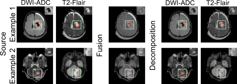
Figure 5: The results from the FusionINN model on closed-source and clinically acquired post-operative image pairs. Clinicians annotated tumor boundaries (highlighted in red), and we display tumor features within green boxes on each image.

3.0.4 Ablation Studies:

Table 2 demonstrates the impact of various parameters on FusionINN’s fusion and decomposition performance. The results indicate that three coupling blocks with $\lambda=0.8$ and $\alpha=0.5$ produce competitive results in terms of $Q_{SSIM}$ scores. Additionally, increasing $\alpha$ enhances image fusion performance with respect to at least one source modality. We also explored different latent priors for $z$, including learning zeros, ones and uniform distribution $\mathcal{U}[0,1)$. The results show that a normally distributed $z$ outperforms other settings, as it might contain more information about the data distribution than, for example, an image containing only zeros. In Fig. 4, the qualitative fusion and decomposition results convey that both $\lambda=0.8$ and $0.9$ prevents under-compensation of $Q_{SSIM}$ via $\ell_{2}$ loss, resulting in superior visual quality.

3.0.5 Clinical Translation:

Fig. 5 illustrates image pairs from DWI-ADC and T2-Flair modalities, depicting post-operative tumor regions of two patients following brain surgery. In this clinical study, medical practitioners sought fused and decomposed images to evaluate the model’s efficacy in aiding prognosis. Specifically, the model was expected to delineate features in T2-Flair indicative of the tumor’s anatomical boundary while preserving high- and low-intensity DWI-ADC features related to residual necrotic and enhancing tumor tissues, respectively. The results show that FusionINN preserves the salient features from both modalities in its decomposed images and effectively combines source features into the fused image. These findings should potentially assist clinicians in making better diagnostic decisions.

4 Conclusion

We introduced a novel framework that integrates the image decomposition task into the fusion problem through the utilization of an invertible and end-to-end normalizing flow network, thereby effectively addressing both optimization tasks with the same model. The bidirectional trainability of FusionINN ensures the robust decomposition of fused images back to their source images using latent image representations. Our framework also showcases its capability in producing clinically relevant fusion and decomposition results. Through extensive evaluation utilizing multiple metrics, FusionINN consistently achieves competitive results when compared to existing generative and discriminative models, while marking itself as the first framework to enable decomposability of fused images. To promote reproducibility and encourage further research, we plan to release the source code of FusionINN, along with other models, evaluation metrics, and pre-processed training data, as open-source.

References

- [1] Bitar, R., Leung, G., Perng, R., Tadros, S., Moody, A. R., Sarrazin, J., McGregor, C., Christakis, M., Symons, S., Nelson, A., Roberts, T.P.: MR pulse sequences: what every radiologist wants to know but is afraid to ask. In: Radiographics, 26(2), 513-537. (2006).
- [2] Xu, Q., Zou, Y., Zhang, X.F.: Sertoli-Leydig cell tumors of ovary: A case series. In: Medicine (Baltimore). 97(42):e12865. (2018).
- [3] Prabhakar, K.R., Srikar, V.S., Babu, R.V.: DeepFuse: A Deep Unsupervised Approach for Exposure Fusion With Extreme Exposure Image Pairs. In: Proceedings of the IEEE International Conference on Computer Vision (ICCV), pp. 4714–4722. (2017)
- [4] Xu, H., Fan, F., Zhang, H., Le, Z., Huang, J.: A deep model for multi-focus image fusion based on gradients and connected regions. IEEE Access 8, 26316–26327 (2020)
- [5] Kumar, N., Hoffmann, N., Oelschlägel, M., Koch, E., Kirsch, M., Gumhold, S.: Structural Similarity Based Anatomical and Functional Brain Imaging Fusion. In: Zhu, D., et al. Multimodal Brain Image Analysis and Mathematical Foundations of Computational Anatomy. MBIA MFCA 2019, 11846. (2019).
- [6] Liu, Y., Chen, X., Cheng, J., Peng, H.: A medical image fusion method based on convolutional neural networks. In: 20th International Conference on Information Fusion (Fusion), 1-7 (2017).
- [7] Zhang, Y., Liu, Y., Sun, P., Yan, H., Zhao, X., Zhang, L.: IFCNN: A general image fusion framework based on convolutional neural network. Information Fusion 54, 99-118 (2020).
- [8] Ma, J., Yu, W., Liang, P., Li, C., Jiang, J.: FusionGAN: A generative adversarial network for infrared and visible image fusion. Information Fusion 48, 11–26 (2019).
- [9] Zhao, Z., Bai, H., Zhu, Y., Zhang, J., Xu, S., Zhang, Y., Zhang, K., Meng, D., Timofte, R., Van Gool, L.: DDFM: Denoising Diffusion Model for Multi-Modality Image Fusion. In: Proceedings of the IEEE/CVF International Conference on Computer Vision (ICCV), 8082-8093. (2023).
- [10] Liu, Y., Chen, X., Wang, Z., Wang, Z. J., Ward, R. K., Wang, X.: Deep learning for pixel-level image fusion: Recent advances and future prospects. Information Fusion 42, 158–173 (2018).
- [11] Zhang, X., Liu, A., Jiang, P., Qian, R., Wei, W., Chen, X.: MSAIF-Net: A Multi-Stage Spatial Attention based Invertible Fusion Network for MR Images. IEEE Transactions on Instrumentation and Measurement. (2023).
- [12] Cui, J., Zhou, L., Li, F., Zha, Y.: Visible and Infrared Image Fusion by Invertible Neural Network. In: China Conference on Command and Control pp. 133–145. (2022).
- [13] Wang, Y., Liu, R., Li, Z., Wang, S., Yang, C., Liu, Q.: Variable Augmented Network for Invertible Modality Synthesis and Fusion. IEEE Journal of Biomedical and Health Informatics. (2023).
- [14] Wang, W., Deng, L. J., Ran, R., Vivone, G.: A General Paradigm with Detail-Preserving Conditional Invertible Network for Image Fusion. International Journal of Computer Vision, 1-26. (2023).
- [15] Zhao, Z., Bai, H., Zhang, J., Zhang, Y., Xu, S., Lin, Z., Timofte, R., Van Gool, L.: Cddfuse: Correlation-driven dual-branch feature decomposition for multi-modality image fusion. In: Proceedings of the IEEE/CVF Conference on Computer Vision and Pattern Recognition pp. 5906–5916. (2023).
- [16] Lu, H., She, Y., Tie, J., Xu, S.: Half-UNet: A Simplified U-Net Architecture for Medical Image Segmentation. Front. Neuroinform. 16:911679. (2022).
- [17] Ronneberger, O., Fischer, P., Brox, T.: U-net: Convolutional networks for biomedical image segmentation. In: Medical Image Computing and Computer-Assisted Intervention–MICCAI 2015: 18th International Conference, Munich, Germany, October 5-9, 2015, Proceedings, Part III 18, 234–-241 (2015).
- [18] Zhou Z, Siddiquee MMR, Tajbakhsh N, Liang J. UNet++: A Nested U-Net Architecture for Medical Image Segmentation. Deep Learn Med Image Anal Multimodal Learn Clin Decis Support (2018).
- [19] Huang, H. et al.: Unet 3+: A full-scale connected unet for medical image segmentation. In: ICASSP 2020-2020 IEEE international conference on acoustics, speech and signal processing (ICASSP), pp. 1055–1059 (2020).
- [20] Dinh, L., Sohl-Dickstein, J., Bengio, S.: Density estimation using Real NVP. In: International Conference on Learning Representations. (2016).
- [21] Wang, Z., Bovik, A. C., Sheikh, H. R., Simoncelli, E. P. Image quality assessment: from error visibility to structural similarity. In: IEEE transactions on image processing, 13(4), 600-612. (2004).
- [22] Petrovic, V., Xydeas, C.: Objective image fusion performance characterisation. In: Tenth IEEE International Conference on Computer Vision (ICCV), 2, 1866–1871, (2005).
- [23] Piella, G., Heijmans, H.: A new quality metric for image fusion. In: Proceedings 2003 International Conference on Image Processing (Cat. No.03CH37429), 3, III–173. (2003).
- [24] Wang, Q., Shen, Y., Jin, J.: 19 - Performance evaluation of image fusion techniques. In: Image Fusion,pp. 469–492. (2008).
- [25] Zhao, H., Gallo, O., Frosio, I., Kautz, J. Loss functions for image restoration with neural networks. In: IEEE Transactions on computational imaging, 3(1), 47-57. (2016).
- [26] Gretton, A., Borgwardt, K.M., Rasch, M.J., Schölkopf, B., Smola, A.: A kernel two-sample test. In: The Journal of Machine Learning Research, 13(1), 723-773. (2012).
- [27] Ardizzone, L., Kruse, J., Rother, C., Köthe, U.: Analyzing Inverse Problems with Invertible Neural Networks. In: International Conference on Learning Representations (ICLR). (2018).
- [28] Haghighat, M.B.A., Aghagolzadeh, A., Seyedarabi, H.: A non-reference image fusion metric based on mutual information of image features. In: Computers & Electrical Engineering, 37(5), 744-756. (2011).
- [29] Menze, B. H., Jakab, A., Bauer, S., Kalpathy-Cramer, J., Farahani, K., Kirby, J. et al.: The Multimodal Brain Tumor Image Segmentation Benchmark (BRATS). In: IEEE Transactions on Medical Imaging, 34(10), 1993-2024. (2015).