Exotic tetraquarks at the HL-LHC with Jethad:
A high-energy viewpoint

Abstract

We review the semi-inclusive hadroproduction of a neutral hidden-flavor tetraquark with light and heavy quark flavor at the HL-LHC, accompanied by another heavy hadron or a light-flavored jet. We make use of the novel TQHL1.0 determinations of leading-twist fragmentation functions to describe the formation mechanism of a tetraquark state within the next-to-leading order perturbative QCD. This framework builds on the basis of a spin-physics inspired model, taken as a proxy for the lowest-scale input of the constituent heavy-quark fragmentation channel. Then, all parton-to-tetraquark fragmentation functions are consistently obtained via the above-threshold DGLAP evolution in a variable-flavor number scheme. We provide predictions for a series of differential distributions calculated by the hands of the Jethad method well-adapted to ${\rm NLL/NLO^{+}}$ hybrid-factorization studies, where the resummation of next-to-leading energy logarithms and beyond is included in the collinear picture. We provide corroborating evidence that high-energy observables sensitive to semi-inclusive tetraquark emissions at the HL-LHC exhibit a fair stability under radiative corrections as well as MHOU studies. Our analysis constitutes a prime contact point between QCD resummations and the exotic matter.

1 Hors d’œuvre

The study of heavy-quark flavored objects in high-energy hadron collisions is crucial for shedding light on the core nature of fundamental interactions. These processes serve as gold-plated channels for probing the underlying dynamics of particle physics. Heavy quarks, due to their large masses, act as sentinels for potential imprints of New Physics, as they could interact with BSM particles. On the other hand, their masses fall within a regime where perturbative QCD calculations are feasible, thus enabling precision studies of strong interactions.

QCD, the theory of the strong force, is a cornerstone of the SM of particle physics. It is based on the non-Abelian $SU(N_{c})$ gauge group, with $N_{c}=3$ representing the number of colors [1, 2, 3, 4]. Quarks, which come in six flavors along with their antiquarks, constitute the building blocks of hadrons. In the QCD framework, quarks are described by fermionic fields belonging to the fundamental triplet representation of $SU(3)$. Gluons, the force carriers of the strong interaction, are massless spin-1 bosons that mediate interactions between quarks. In the QCD Lagrangian, gluons are represented by bosonic fields belonging to the adjoint octet representation of $SU(3)$.

While QCD stands as one of the fundamental pillars of the SM, it also serves as a fertile ground for probing BSM physics. Several potential portals to BSM extensions within the realm of QCD have been proposed. Among others, they include: axions, which were originally postulated to address the strong CP problem [5, 6, 7, 8], non-Abelian dark gauge forces [9, 10], quarkyonic matter [11, 12, 13], and higher-dimensional QCD operators incorporated into the Lagrangian [14, 15, 16, 17]. This wealthy of possibilities provide us with rich opportunities for exploring the frontiers of particle physics and searching for long-awaited signs of physics beyond the SM.

Within the QCD domain, a key role is played by hadrons whose lowest Fock state contains two or more heavy quarks. Mesons composed of a heavy quark ($Q$) and its antiquark ($\bar{Q}$) are known as (heavy) quarkonia. The origins of quarkonium studies trace back to the so-called “Quarkonium November Revolution”. Indeed, in November 1974, a groundbreaking discovery was made: a new vector meson, with a mass around 3.1 GeV and carrying photon quantum numbers, was observed independently by two research groups. This meson was named $J/\psi$, after the two institutions where it was discovered: the Stanford Linear Accelerator Center (SLAC) led by B. Richter [18], and the Brookhaven National Laboratory (BNL) led by S. Ting [19]. Shortly after these announcements, the discovery of the $J/\psi$ was confirmed by the Frascati ADONE experiment, under the direction of G. Bellettini [20]. This landmark heralded the beginning of quarkonium studies and provided crucial insights into the nature of the strong force and the underlying quark structure of hadrons.

Though quarkonium mesons fall into the class of ordinary hadrons, QCD color neutrality allows for the formation of bound states with more intricate valence-parton configurations, leading to the emergence of exotic hadrons. These exotic particles have quantum numbers that cannot be explained by conventional quark-antiquark or three-quark configurations. Instead, they are composed of unique combinations of quarks, antiquarks, and gluons. Understanding the inner structure of these exotic hadrons has been the focus of intense research in the field of exotic spectroscopy. Exotic hadrons can be classified into two main categories: those composed of active gluons, such as quark-gluon hybrids [21, 22, 23] (see also Refs. [24, 25, 26, 27, 28]) and glueballs [29, 30, 31, 32, 33, 34, 35, 36, 37], and those composed of multiple quarks, such as tetraquarks and pentaquarks [2, 38, 39, 40].

The observation of the first exotic hadron, the $X(3872)$, occurred in 2003 at the Belle experiment [41], and subsequent experiments confirmed its existence. Its discovery marked the beginning of the so-called “Second Quarkonium Revolution”, or “Exotic Revolution”. The $X(3872)$ is a hidden-charm particle, believed to be composed of charm and anticharm quarks [42, 43, 44]. The first exotic state with open-charm flavor, the $X(2900)$ particle, was observed for the first time in 2021 at LHCb [45]. Although the $X(3872)$ has quantum numbers that are not exotic, its decay properties violate isospin conservation, suggesting that its inner structure may involve more complex dynamics beyond traditional quarkonium states. Various theoretical models have been proposed to describe the $X(3872)$, including a loosely-bound meson molecule [46, 47, 48, 49, 50, 51, 52, 53, 54, 55, 56, 57, 58, 59], a compact diquark system [60, 61, 62, 63, 64, 65, 66, 67, 68], or a hadroquarkonium configuration consisting of a quarkonium core and an orbiting light meson [69, 70, 71, 72, 73, 74, 75, 76].

Quite recently, a high-energy description of the single hadroproduction of fully charmed tetraquarks was proposed [77, 78]. The production rates of the $X(3872)$ at large transverse momenta, as measured by experiments at the LHC, provide valuable insights into its production mechanisms. These measurements can help to constrain theoretical models and favor production mechanisms inherent in high-energy QCD, such as the fragmentation of a single parton into the observed particle.

In this review we address the associated hadroproduction, at LHC and its high-luminosity upgrade (HL-LHC), of a forward heavy-light tetraquark and a backward singly heavy-flavored hadron or a light jet. The two outgoing particles possesses high transverse momenta and a large mutual separation in rapidity. On the one side, the presence of moderate parton longitudinal-momentum fractions allows for a reliable description using collinear PDFs. On the other side, large rapidity intervals in the final state lead to significant exchanges of transverse momenta in the $t$-channel.

Therefore, a high-energy factorization treatment, accounting for energy logarithms due to $t$-channel gluon emissions, becomes necessary. With the aim of providing an accurate high-energy QCD description of our reactions in these kinematic ranges, we rely upon the Jethad method [79, 80, 81] to implement the ${\rm NLL/NLO^{+}}$ hybrid-factorization formalism [82, 79, 83, 84, 80, 85, 81], in which the resummation of next-to-leading energy logarithms and beyond is consistently included in the collinear picture.

Then, the last required ingredient is the choice of a reliable mechanism depicting the formation of our heavy-light tetraquark states in the kinematic regimes of interest. From a collinear-factorization viewpoint, the transverse momenta at which final-state particles are tagged make the use of a VFNS approach [86, 87] valid.

To this extent, we will make use of a novel set of collinear FFs, named TQHL1.0, suited to the VFNS fragmentation of $X_{Qq\bar{Q}\bar{q}}$ tetraquarks [88]. They were obtained by performing a next-to-leading DGLAP evolution of an initial-scale input for the constituent heavy-quark fragmentation channel, obtained within the spin-physics inspired SNAJ model [89, 90, 91, 92].

For the sake of completeness, we mention that other hybrid-factorization formalisms, closely related to our ${\rm NLL/NLO^{+}}$ framework and tailored for single forward detections, exist. These include the approaches proposed in Refs. [93, 94, 95, 96, 97, 98, 99], which offer valuable insights and can complement our approach in understanding high-energy QCD processes.

On the other side, analyses on small-$x$ resummed inclusive or differential distributions for Higgs and heavy-flavor hadroproduction have been conducted using the Hell method [100, 101]. The Hell method relies on the ABF approach [102, 103, 104, 105, 106, 107, 108], which combines collinear factorization with small-$x$ resummation, along with high-energy factorization theorems [109, 110, 111, 112, 113, 114, 115, 116]. These analyses offer complementary perspectives and contribute to a more comprehensive understanding of high-energy QCD phenomena.

The outline of this review reads as follows. In Section 2 we introduce the ${\rm NLL/NLO^{(+)}}$ hybrid collinear and high-energy factorization, whereas in we Section 3 we provide technical details on our strategy to describe tetraquark collinear fragmentation. Results and conclusions are presented in Sections 4 and 5, respectively.

2 Theoretical setup

This Section is for a digression on recent phenomenological progresses of high-energy resummation in QCD (see Section 2.1). Then, it gives a formal description of the observables matter of our analysis as cast within the hybrid factorization (see Section 2.2).

2.1 High-energy QCD phenomenology: An incomplete summary

Providing accurate predictions for high-energy observables relies upon the ability to disentangle long-distance from short-distance dynamics in hadron scatterings. This permits to factorize nonperturbative dynamics from perturbative calculations via the well-established collinear framework [117, 118].

However, specific kinematic regions pose challenges due to the emergence of large logarithms. These logarithmic corrections grows with the order of the perturbative expansion, thus offsetting the smallness of the QCD running coupling and hampering the convergence of perturbative series. In such scenarios, the standard collinear factorization must be enhanced via the incorporation of all-order resummations.

In the semi-hard regime of QCD [119] (see Refs. [120, 121, 122] for advances in phenomenology), characterized by a stringent energy scale hierarchy $\sqrt{s}\gg{Q}\gg\Lambda_{\rm QCD}$, large logarithms of the form $\ln s/Q^{2}$ enter perturbative series with a power increasing with the order, thus calling for a resummation treatment.

The BFKL formalism [123, 124, 125, 126] proves to be the most adequate tool for high-energy resummation. More in particular, BFKL allows us to resum all contributions proportional to $(\alpha_{s}\ln s)^{n}$, the so-called LL approximation, as well as the ones going with to $\alpha_{s}(\alpha_{s}\ln s)^{n}$, namely the next-to-leading logarithmic NLL approximation.

According to BFKL, a given scattering amplitude factorizes as a convolution between a universal Green’s function and two singly-off-shell, transverse-momentum dependent emission functions (also known as impact factors) describing the emission of a forward particle from the fragments of the corresponding parent hadron. Using the BFKL jargon, these coefficients are also known as forward-production impact factors. The Green’s function is governed by an integral evolution equation, whose kernel is known at the NLO perturbative accuracy [127, 128, 129, 130, 131, 132, 133] (see Refs. [134, 135, 136, 137, 138, 139] for ongoing efforts in calculating higher-order corrections).

The predictive capability of the high-energy resummation from BFKL at NLL is constrained by the availability of off-shell emission functions computed within NLO. They include: a) colliding-parton (quarks and gluons) impact factors [140, 141], which are needed to calculate b) forward-jet [142, 143, 144, 145, 146, 147] and c) forward light hadron [148] emission functions. Additionally, we mention: d) virtual photon to light vector meson [149], e) light-by-light impact factors [150, 151, 152, 153, 154, 155], and f) the emission function for the production of a forward Higgs boson in the infinite top-mass limit [156, 157] (see also Refs. [158, 159]). Staying at LO, we include: Drell–Yan pairs [160, 161], heavy-quark pairs [162, 163, 164], and forward $J/\psi$ emitted at low transverse momentum [165] (see also Refs. [166, 167, 168]).

Gold-plated phenomenological channels to probe high-energy QCD dynamics at hadron colliders essentially fall into the following classes: Mueller–Navelet dijets [169, 82, 145, 170, 171, 172, 173, 147, 174, 175, 176, 177, 178, 179, 180, 181, 182], dihadron production [183, 184, 185, 186, 187] and multi-jet tags [188, 189, 190, 191, 192, 193, 194, 195, 196, 197, 198, 199, 200, 201], hadron plus jet [202, 203, 204, 79, 205, 206], Higgs plus jet [83, 207, 208, 209, 210], heavy-light dijet systems [84, 211] and heavy-hadron [165, 162, 212, 164, 163, 213, 214, 215, 85, 216, 217, 218, 219, 220, 221] emissions.

Remarkably, detections of single forward particles are excellent probe channels for the proton’s content at low-$x$ through the BFKL Unintegrated Gluon Distribution (UGD), whose energy evolution is ruled by the BFKL Green’s function. We mention: light vector-meson leptoproduction at HERA [222, 223, 224, 225, 226, 227, 228, 229, 230] and the Electron-Ion Collider (EIC) [231, 232, 233, 234, 235], exclusive quarkonium photoproduction [236, 237, 238, 239], and the inclusive detection of Drell–Yan dilepton systems [161, 240, 241, 242].

The information on the gluon content at small-$x$ provided by the BFKL UGD turned out to be decisive to improve the description of small-$x$ resummed collinear PDFs [243, 244, 245]. Additionally, it connects with model studies of low-$x$ improved, twist-two gluon TMD distributions [246, 247, 248, 249, 250, 251, 252, 253, 254, 255, 256]. Analyses presented in Refs. [257, 258] provide insights into the relationship between TMD and low-$x$ dynamics. Studies in Refs. [259, 260] delve into the exploration of the connection between the UGD and color-dipole cross sections.

A striking challenge connected to the BFKL description of Mueller–Navelet rapidity distributions and azimuthal-angle correlations arises from the impact of NLL contributions. These NLL terms, while of the same order as the pure LL case, exhibit an opposite sign. This leads to strong instabilities within the resummed series, particularly when studies on MHOUs via variations of energy scales around their natural values are made.

Consequently, Mueller–Navelet observables tend to assume unphysical values, especially as the rapidity separation between jets becomes sufficiently large. Likewise, azimuthal correlations display anomalous behaviors at both small and large rapidity distances. Various approaches have been explored to address this issue. Notably, the BLM prescription [261, 262, 263, 264], specifically designed for semi-hard processes [174], provides a partial mitigation of these instabilities in azimuthal correlations, leading to a moderate improvement in agreement with experimental data.

However, the efficacy of BLM is limited, particularly in the case of light dihadron or hadron plus jet semi-hard distributions. The primary reason for this limitation is that the optimal renormalization scale values recommended by BLM are significantly higher than the natural scales of the underlying processes [120, 202, 79]. Consequently, in these scenarios total cross sections suffer from a substantial reduction in statistics.

Compelling indications of a reached stabilization of the high-energy resummation under higher-order corrections and scale variations have been recently observed in the context of semi-hard reactions featuring final states sensitive to Higgs boson detections [83, 265, 266, 267, 268, 269, 270, 271]. A clear signature of this stabilizing trend came out for the first time from studies on the semi-inclusive emissions of $\Lambda_{c}$ hyperons [213] or singly bottomed hadrons [214] at the LHC. In particular, it was highlighted that the stabilizing effect is directly connected with the distinctive pattern exhibited by VFNS collinear FFs governing the production of these singly heavy-flavored particles at high transverse momentum.

Subsequent analyses on vector quarkonia [85, 81], charmed $B$ mesons [218, 221], and heavy-light tetraquarks [88], clarified that this remarkable property, known as natural stability of the high-energy resummation in QCD [216], emerges as an intrinsic feature inherently associated with final states sensitive to heavy flavor.

2.2 Hybrid-factorization studies at ${\rm NLL/NLO}$ and beyond

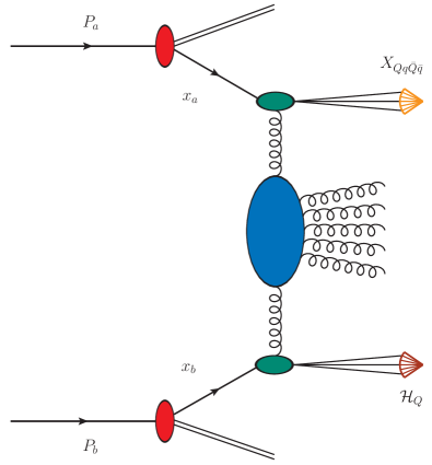
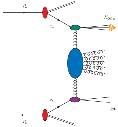
Figure 1: Pictorial representation of the tetraquark $+$ hadron (left) and tetraquark $+$ jet (right) semi-inclusive hadroproduction within the hybrid collinear and high-energy factorization (figures realized with JaxoDraw 2.0 [272]). Red blobs depict collinear FFs. The off-shell hard factor, part of the hadron (jet) emission function, is given by green (violet) ovals. Tetraquark ($Q$-hadron) emissions are portrayed by orange (firebrick) arrows. The large blue blob at the center of each diagram represents the BFKL Green’s function.

We investigate the two classes of processes represented in Fig. 1

$$\begin{split}{\rm p}(P_{a})\;+\;{\rm p}(P_{b})&\;\rightarrow\;X_{Qq\bar{Q}\bar{q}}(\bm{\kappa}_{1},y_{1})\;+\;{\cal X}\;+\;{\cal H}_{Q}(\bm{\kappa}_{2},y_{2})\;,\\ {\rm p}(P_{a})\;+\;{\rm p}(P_{b})&\;\rightarrow\;X_{Qq\bar{Q}\bar{q}}(\bm{\kappa}_{1},y_{1})\;+\;{\cal X}\;+\;{\rm jet}(\bm{\kappa}_{2},y_{2})\;,\end{split}$$ (1)

where a heavy-light tetraquark ($X_{cu\bar{c}\bar{u}}$, $X_{cs\bar{c}\bar{s}}$, $X_{bu\bar{b}\bar{u}}$, or $X_{bs\bar{b}\bar{s}}$) is emitted in association with singly heavy-flavored hadron (${\cal H}_{c}$ or ${\cal H}_{b}$), or a light jet, ${\cal O}=\{{\cal H}_{c},{\cal H}_{b},{\rm jet}\}$. The final-state particles possess large transverse momenta, $|\bm{\kappa}_{1,2}|\gg\Lambda_{\rm QCD}$, and their rapidity separation is $\Delta Y\equiv y_{1}-y_{2}$.

As for a ${\cal H}_{c}$ hadron, we refer to inclusive states consisting in the sum of fragmentation channels to single-charmed $D^{\pm}$, $D^{0}$ and $D^{*\pm}$ mesons, and also $\Lambda_{c}^{\pm}$ hyperons. Analogously, a ${\cal H}_{b}$ particle stands as combinations of noncharmed $B$ mesons and $\Lambda_{b}^{0}$ baryons [214]. The undetected gluon radiation is inclusively indicated as ${\cal X}$. Large observed transverse momenta and large rapidity distances are needed for dealing with semi-hard final-state configurations. Furthermore, transverse-momentum ranges have to be large enough to make the validity of the VFNS collinear fragmentation be the dominant mechanism for the production of heavy hadrons.

Incoming protons’ four-momenta can decomposed as Sudakov vectors satisfying $P_{a}^{2}=P_{b}^{2}=0$ and $2(P_{a}\cdot P_{b})=s$. In this way, $\kappa_{1}$ and $\kappa_{2}$ can be cast as

$$\kappa_{1,2}=x_{1,2}P_{a,b}-\frac{\kappa_{1,2\perp}^{\,2}}{x_{1,2}s}P_{b,a}+\kappa_{1,2\perp}\ ,\qquad\bm{\kappa}_{1,2}^{\,2}\equiv-\kappa_{1,2\perp}^{2}\;.$$ (2)

Final-state object’s longitudinal fractions, $x_{1,2}$, depend on rapidities as $y_{1,2}=\pm\frac{1}{2}\ln\frac{x_{1,2}^{2}s}{\bm{\kappa}_{1,2}^{2}}$. Thus one have ${\rm d}y_{1,2}=\pm\frac{{\rm d}x_{1,2}}{x_{1,2}}$, and $\Delta Y\equiv y_{1}-y_{2}=\ln\frac{x_{1}x_{2}s}{|\bm{\kappa}_{1}||\bm{\kappa}_{2}|}$.

The LO cross section of our reactions (Eq. (1)) in pure collinear QCD would take the form of a one-dimensional convolution among protons’ PDFs, hadrons’ FFs, and partonic hard factors. In the double hadron channel (panel a) of Fig. 1), one writes

$$\begin{split}\frac{{\rm d}\sigma_{[p\;+\;p\;\;\to\;\;X_{Qq\bar{Q}\bar{q}}\;+\;{\cal H}_{Q}]}^{\rm LO}}{{\rm d}x_{1}{\rm d}x_{2}{\rm d}^{2}\bm{\kappa}_{1}{\rm d}^{2}\bm{\kappa}_{2}}&=\sum_{a,b}\int_{0}^{1}{\rm d}x_{a}\int_{0}^{1}{\rm d}x_{b}\ f_{a}(x_{a},\mu_{F})f_{b}(x_{b},\mu_{F})\\ &\times\,\int_{x_{1}}^{1}\frac{{\rm d}z_{1}}{z_{1}}\int_{x_{2}}^{1}\frac{{\rm d}z_{2}}{z_{2}}\ D^{X}_{a}\left(\frac{x_{1}}{z_{1}},\mu_{F}\right)D^{\cal H}_{b}\left(\frac{x_{2}}{z_{2}},\mu_{F}\right)\frac{{\rm d}{\hat{\sigma}}_{a,b}}{{\rm d}x_{a}{\rm d}x_{b}{\rm d}z_{1}{\rm d}z_{2}{\rm d}^{2}\bm{\kappa}_{1}{\rm d}^{2}\bm{\kappa}_{2}}\;,\end{split}$$ (3)

where ($a,b$) indices run over quarks, antiquarks, and the gluon, $f_{a,b}$ are proton PDFs, $D^{X}_{a,b}$ $\big{(}D^{\cal H}_{a,b}\big{)}$ denote heavy-light tetraquark (singly heavy-flavored hadron) FFs, $x_{a,b}$ stand for the longitudinal fractions of the struck partons, $z_{1,2}$ are the longitudinal fractions of outgoing partons, and ${\rm d}\hat{\sigma}_{a,b}$ are partonic-subprocess cross sections.

Analogously, in the tetraquark plus jet channel (panel b) of Fig. 1) we have

$$\begin{split}\frac{{\rm d}\sigma_{[p\;+\;p\;\;\to\;\;{X_{Qq\bar{Q}\bar{q}}}\;+\;{\rm jet}]}^{\rm LO}}{{\rm d}x_{1}{\rm d}x_{2}{\rm d}^{2}\bm{\kappa}_{1}{\rm d}^{2}\bm{\kappa}_{2}}&=\sum_{a,b}\int_{0}^{1}{\rm d}x_{a}\int_{0}^{1}{\rm d}x_{b}\ f_{a}(x_{a},\mu_{F})f_{b}(x_{b},\mu_{F})\int_{x_{1}}^{1}\frac{{\rm d}z}{z}D^{X}_{a}\left(\frac{x_{1}}{z}\right)\frac{{\rm d}{\hat{\sigma}}_{a,b}}{{\rm d}x_{1}{\rm d}x_{2}{\rm d}z\,{\rm d}^{2}\bm{\kappa}_{1}{\rm d}^{2}\bm{\kappa}_{2}}\;.\end{split}$$ (4)

On the contrary, deriving the formula for the high-energy resummed cross section within our hybrid factorization requires a two-step process. First, we employ the high-energy factorization as prescribed by BFKL. Then, we enhance the description by incorporating collinear components, PDFs and FFs. To this extent, we express the differential cross section as a Fourier sum of azimuthal-angle coefficients

$$\frac{{\rm d}\sigma^{\rm NLL/NLO^{+}}}{{\rm d}y_{1}{\rm d}y_{2}{\rm d}\bm{\kappa}_{1}{\rm d}\bm{\kappa}_{2}{\rm d}\varphi_{1}{\rm d}\varphi_{2}}=\frac{1}{(2\pi)^{2}}\left[{\cal C}_{0}^{\rm NLL/NLO^{+}}+2\sum_{n=1}^{\infty}\cos\left(n(\Phi-\pi)\right)\,{\cal C}_{n}^{\rm NLL/NLO^{+}}\right]\,,$$ (5)

with $\varphi_{1,2}$ the observed azimuthal angles and $\Phi\equiv\varphi_{1}-\varphi_{2}$. Azimuthal coefficients are calculated within the BFKL formalism and they encode the LL and NLL resummation of high-energy logarithms. We rely upon the $\overline{\rm MS}$ renormalization scheme [273] to write (see Ref. [145] for details)

$$\begin{split}{\cal C}_{n}^{\rm NLL/NLO^{+}}&=\int_{0}^{2\pi}{\rm d}\varphi_{1}\int_{0}^{2\pi}{\rm d}\varphi_{2}\,\cos\left(n(\Phi-\pi)\right)\,\frac{{\rm d}\sigma^{\rm NLL/NLO^{+}}}{{\rm d}y_{1}{\rm d}y_{2}\,{\rm d}|\bm{\kappa}_{1}|\,{\rm d}|\bm{\kappa}_{2}|{\rm d}\varphi_{1}{\rm d}\varphi_{2}}\;\\ &=\;\frac{e^{\Delta Y}}{s}\int_{-\infty}^{+\infty}{\rm d}\nu\,e^{{\Delta Y}\bar{\alpha}_{s}(\mu_{R})\chi^{\rm NLO}(n,\nu)}\\ &\times\;\alpha_{s}^{2}(\mu_{R})\,\biggl{\{}{\cal F}_{1}^{\rm NLO}(n,\nu,|\bm{\kappa}_{1}|,x_{1})[{\cal F}_{2}^{\rm NLO}(n,\nu,|\bm{\kappa}_{2}|,x_{2})]^{*}\,\\ &+\,\left.\bar{\alpha}_{s}^{2}(\mu_{R})\,\Delta Y\frac{\beta_{0}}{4N_{c}}\chi(n,\nu)f(\nu)\right\}\;,\end{split}$$ (6)

where $\bar{\alpha}_{s}(\mu_{R})\equiv\alpha_{s}(\mu_{R})N_{c}/\pi$ with $N_{c}$ the color number, $\beta_{0}=11N_{c}/3-2n_{f}/3$ is the first coefficient of the QCD $\beta$-function with $n_{f}$ the flavor number. We select a two-loop running coupling with initial condition $\alpha_{s}\left(M_{Z}\right)=0.11707$ and a dynamic $n_{f}$. The BFKL kernel at the exponent of Eq. (6) reads

$$\chi^{\rm NLO}(n,\nu)=\chi(n,\nu)+\bar{\alpha}_{s}\hat{\chi}(n,\nu)\;,$$ (7)

with

$$\chi\left(n,\nu\right)=-2\gamma_{\rm E}-2\,{\rm Re}\left\{\psi\left(\frac{1+n}{2}+i\nu\right)\right\}\,$$ (8)

being the LO BFKL eigenvalues, $\gamma_{\rm E}$ the Euler-Mascheroni constant, and $\psi(z)\equiv\Gamma^{\prime}(z)/\Gamma(z)$ the logarithmic derivative of the Gamma function. The $\hat{\chi}(n,\nu)$ function in Eq. (7) is the NLO kernel correction

$$\begin{split}\hat{\chi}\left(n,\nu\right)&=\bar{\chi}(n,\nu)+\frac{\beta_{0}}{8N_{c}}\chi(n,\nu)\left(-\chi(n,\nu)+10/3+2\ln\frac{\mu_{R}^{2}}{\mu_{C}^{2}}\right)\;,\end{split}$$ (9)

with $\mu_{C}\equiv\sqrt{m_{1\perp}m_{2\perp}}$, where $m_{(1,2)\perp}$ are the observed-particle transverse masses. Masses or our heavy-light tetraquark are set to $m_{X}=2(m_{q}+m_{Q})$, with $M_{q}$ ($m_{Q}$) being the mass of the light (heavy) constituent quark. The transverse mass of the light-flavored jet merely coincides with its transverse momentum, $|\bm{\kappa}_{J}|$. The characteristic $\bar{\chi}(n,\nu)$ function was obtained in Ref. [274]

$$\bar{\chi}(n,\nu)\,=\,-\frac{1}{4}\left\{\frac{\pi^{2}-4}{3}\chi(n,\nu)-6\zeta(3)-\frac{{\rm d}^{2}\chi}{{\rm d}\nu^{2}}+\,2\,\phi(n,\nu)+\,2\,\phi(n,-\nu)\right.$$ (10)

$$\left.+\;\frac{\pi^{2}\sinh(\pi\nu)}{2\,\nu\,\cosh^{2}(\pi\nu)}\left[\left(3+\left(1+\frac{n_{f}}{N_{c}^{3}}\right)\frac{11+12\nu^{2}}{16(1+\nu^{2})}\right)\delta_{n0}-\left(1+\frac{n_{f}}{N_{c}^{3}}\right)\frac{1+4\nu^{2}}{32(1+\nu^{2})}\delta_{n2}\right]\right\}\,,$$

with

$$\phi(n,\nu)\,=\,-\int_{0}^{1}{\rm d}x\,\frac{x^{-1/2+i\nu+n/2}}{1+x}\left\{\frac{1}{2}\left(\psi^{\prime}\left(\frac{n+1}{2}\right)-\zeta(2)\right)+\mbox{Li}_{2}(x)+\mbox{Li}_{2}(-x)\right.$$ (11)

$$\left.+\;\ln x\left[\psi(n+1)-\psi(1)+\ln(1+x)+\sum_{k=1}^{\infty}\frac{(-x)^{k}}{k+n}\right]+\sum_{k=1}^{\infty}\frac{x^{k}}{(k+n)^{2}}\left[1-(-1)^{k}\right]\right\}$$

$$=\;\sum_{k=0}^{\infty}\frac{(-1)^{k+1}}{k+(n+1)/2+i\nu}\left\{\psi^{\prime}(k+n+1)-\psi^{\prime}(k+1)\right.$$

$$\left.+\;(-1)^{k+1}\left[\beta_{\psi}(k+n+1)+\beta_{\psi}(k+1)\right]-\frac{\psi(k+n+1)-\psi(k+1)}{k+(n+1)/2+i\nu}\right\}\;,$$

where

$$\beta_{\psi}(z)=\frac{1}{4}\left[\psi^{\prime}\left(\frac{z+1}{2}\right)-\psi^{\prime}\left(\frac{z}{2}\right)\right]\;,$$ (12)

and

$$\mbox{Li}_{2}(x)=\int^{x}_{0}{\rm d}\omega\,\frac{\ln(1-\omega)}{\omega}\;.$$ (13)

The singly off-shell emissions functions

$${\cal F}_{1,2}^{\rm NLO}(n,\nu,|\bm{\kappa}_{1,2}|,x_{1,2})={\cal F}_{1,2}(n,\nu,|\bm{\kappa}_{1,2}|,x_{1,2})+\alpha_{s}(\mu_{R})\,\hat{\cal F}_{1,2}(n,\nu,|\bm{\kappa}_{1,2}|,x_{1,2})$$ (14)

The LO expressions for these functions depicting the production of a forward hadron and a forward jet respectively read as

$$\begin{split}{\cal F}_{h}(n,\nu,|\bm{\kappa}_{h}|,x_{h})&=2\,\sqrt{\frac{C_{F}}{C_{A}}}|\bm{\kappa}_{h}|^{2i\nu-1}\,\int_{x_{h}}^{1}\frac{{\rm d}z}{z}\left(\frac{z}{x_{h}}\right)^{2i\nu-1}\left[\frac{C_{A}}{C_{F}}f_{g}(z)D_{g}^{h}\left(\frac{x_{h}}{z}\right)+\sum_{a=q,\bar{q}}f_{a}(z)D_{a}^{h}\left(\frac{x_{h}}{z}\right)\right]\end{split}$$ (15)

and

$${\cal F}_{J}(n,\nu,|\bm{\kappa}_{J}|,x_{J})=2\sqrt{\frac{C_{F}}{C_{A}}}|\bm{\kappa}_{J}|^{2i\nu-1}\,\left[\frac{C_{A}}{C_{F}}f_{g}(x_{J})+\sum_{b=q,\bar{q}}f_{b}(x_{J})\right]\;,$$ (16)

with $C_{F}\equiv(N_{c}^{2}-1)/(2N_{c})$ and $C_{A}\equiv N_{c}$ the usual Casimir QCD factors. The $f(\nu)$ function is related to a logarithmic derivative of LO emission functions

$$f(\nu)=\frac{i}{2}\,\frac{{\rm d}}{{\rm d}\nu}\ln\left(\frac{{\cal F}_{1}}{{\cal F}_{2}^{*}}\right)+\ln\left(|\bm{\kappa}_{1}||\bm{\kappa}_{2}|\right)\;.$$ (17)

In Eq. (6), the remaining components are the NLO emission-function corrections, denoted as $\hat{\cal F}_{1,2}$. The forward-hadron NLO term is determined under the was calculated in Ref. [148] and its expression is provided in Appendix A of this review. As for the forward-jet NLO term, our choice follows Refs. [148, 146]. To ease numerical analyses, we employ a jet selection function calculated within the SCA [279, 280] in its cone-type version [147] and with the jet cone radius set to ${\cal R}=0.5$. The analytic expression for this emission function is given in Appendix B.

A proper way for a phenomenological comparison between our hybrid factorization and pure fixed-order results would necessitate for a numerical framework tailored for computing NLO distributions two-particle reactions in hadron collisions. According to our knowledge, such a technology is currently unavailable. For the sake of comparison with reference fixed-order predictions, we truncate the expansion of azimuthal coefficients of Eq. (6) up to the ${\cal O}(\alpha_{s}^{3})$ levels. This gives us an effective high-energy fixed-order (${\rm HE}\mbox{-}{\rm NLO^{+}}$) expression, which captures the leading-power asymptotic signal present an pure NLO calculation and, at the same time, disregards terms proportional to inverse powers of the partonic center-of-mass energy. The $\overline{\rm MS}$ expressions for the azimuthal coefficients at ${\rm HE}\mbox{-}{\rm NLO^{+}}$ reads

$${\cal C}_{n}^{{\rm HE}\text{-}{\rm NLO}^{+}}=\frac{e^{\Delta Y}}{s}\int_{-\infty}^{+\infty}{\rm d}\nu\,\alpha_{s}^{2}(\mu_{R})\,\left[1+\bar{\alpha}_{s}(\mu_{R})\Delta Y\chi(n,\nu)\right]\,{\cal F}_{1}^{\rm NLO}(n,\nu,|\bm{\kappa}_{1}|,x_{1})\,[{\cal F}_{2}^{\rm NLO}(n,\nu,|\bm{\kappa}_{2}|,x_{2})]^{*}\;,$$ (18)

with the exponentiated kernel expanded and truncated at ${\cal O}(\alpha_{s})$. Moreover, we present predictions at a pure LL order, given by

$${\cal C}_{n}^{\rm LL/LO}=\frac{e^{\Delta Y}}{s}\int_{-\infty}^{+\infty}{\rm d}\nu\,e^{{\Delta Y}\bar{\alpha}_{s}(\mu_{R})\chi(n,\nu)}\,\alpha_{s}^{2}(\mu_{R})\,{\cal F}_{1}(n,\nu,|\bm{\kappa}_{1}|,x_{1})[{\cal F}_{2}(n,\nu,|\bm{\kappa}_{2}|,x_{2})]^{*}\,.$$ (19)

Eqs. (6) to (19) tells us the way our hybrid factorization is constructed. According to BFKL, the hadronic cross section is high-energy factorized as a transverse-momentum convolution between the Green’s function and the two off-shell emission functions. These impact factors embody collinear PDFs and FFs. The ${\rm NLL/NLO^{+}}$ label emphasizes the complete resummation of energy logarithms at NLL accuracy by means of perturbative ingredients calculated at NLO. The ‘$+$’ superscript in Eq. (6) highlights the fact that some next-to-NLL contributions, resulting from the cross product of the two NLO impact-factor corrections, are also accounted for.

Renormalization ($\mu_{R}$) and factorization ($\mu_{F}$) scales are set to the natural energies suggested by process kinematics. Thus, we have $\mu_{R}=\mu_{F}=\mu_{N}=m_{1\perp}+m_{2\perp}$. As for collinear PDFs, we make use of the NNPDF4.0 NLO set [281, 282] as implemented in the LHAPDF v6.5.4 interface [283]. Such PDFs were extracted by means of global fits and through the so-called replica method, originally derived in Ref. [284] in the context of neural-network techniques and now widely employed on multi-dimensional analyses of the proton structure [285, 286, 287, 288, 289, 290] (see Ref. [291] for a quantitative study on ambiguities emerging from correlations among different PDF sets). All calculations presented in this review are performed in the $\overline{\rm MS}$ renormalization scheme [273].

3 Heavy-flavor fragmentation: From heavy-light hadrons to tetraquarks

In this Section we present our strategy to depict inclusive emissions heavy-flavored hadrons via the VFNS collinear fragmentation. Section 3.1 is for a digression on the emergence of the natural stability [216]. Features of the novel TQHL1.0 FF determinations for heavy-light tetraquark state are discussed in detail in Section 3.2.

3.1 Rise and discovery of the natural stability

The direct link between the dynamics governing DGLAP-evolving VFNS FFs and the stabilization pattern of the hybrid factorization was initially uncovered via studies of semi-hard emissions of singly heavy-flavored hadrons, including $D$ mesons [292, 293, 294, 295, 296, 297, 298, 299, 300], $\Lambda_{c}$ hyperons [293, 301, 302], and $b$-flavored (${\cal H}_{b}$) hadrons [303, 304, 305, 306, 307, 308, 309, 310, 311].

A surprising and unexpected stabilizing trend under MHOU studies came out in observables sensitive to the forward semi-inclusive emission of $\Lambda_{c}$[213, 80, 215], $D^{*\pm}$[219, 217], and ${\cal H}_{b}$[214, 80] particles. It was then confirmed by analyses of vector quarkonia and charmed $B$ mesons produced via the single-parton (leading-twist) fragmentation mechanism relying upon an initial-scale input [312, 313, 314, 315, 316, 317, 318, 319, 320]. Contextually, novel determinations of DGLAP-evolving FFs for vector quarkonia and $B_{c}^{(*)}$ mesons were obtained in Refs. [85, 220] and [218], respectively. A weaker, but still present stabilization trend also rises when $s$-flavored, cascade $\Xi^{-}/\bar{\Xi}^{+}$ baryons are detected [206].

The main outcome of Refs. [216, 213, 214, 85, 218] was a clear indication that gluon collinear FF channel has a crucial role in our NLL hybrid factorization framework. Its energy dependence is responsible for the stability of the high-energy logarithmic series in our observables. Specifically, in the kinematic sectors of interest, where $10^{-4}\lesssim x\lesssim 10^{-2}$, the gluon PDF dominates over all (anti)quark channels. Since the gluon FF is convoluted diagonally with the gluon PDF in the LO hadron impact factor (see Eq.(15)), its behavior is significantly amplified. This characteristic persists even at NLO [214], when the $(qg)$ and $(gq)$ nondiagonal channels are active (see AppendixA).

While the QCD running coupling decreases with $\mu_{R}$, and this affects both the Green’s function and the impact factors, it is well-known that the gluon PDF grows with $\mu_{F}$. When the latter is convoluted in the emission function with a gluon FF that also increases with $\mu_{F}$, as it happens for heavy-flavored hadrons, these two effects counteract each other. The net results is a stabilizing trend of heavy-hadron distributions under MHOU studies. The more pronounced the growth with $\mu_{F}$ of the gluon FF, the clearer the stabilization pattern becomes. This is the reason why distributions sensitive to singly bottom-flavored states are generally more stable charm-sensitive ones [214]. In contrast, when the gluon FF decreases with $\mu_{F}$, as observed for lighter hadron species [213, 206, 221], no stabilization under MHOU is evident. This hampers any possibility of conducting precision studies of high-energy distributions at natural energy scales [79].

The manifestation of natural stability in the presence of both singly heavy-flavored hadrons or quarkonia clearly highlights that this remarkable property is an intrinsic characteristic of heavy-flavor emissions. It becomes apparent whenever a heavy-hadron species is detected and it does not depend on the basis assumptions made to build corresponding collinear FFs.

3.2 The TQHL1.0 FF determinations

Here we present our TQHL1.0 functions. They are VFNS, DGLAP-evolved collinear FFs describing the direct inclusive production of a $S$-wave $X_{Qq\bar{Q}\bar{q}}$ tetraquark state within the single-parton, leading-twist fragmentation mechanism. We essentially follow a two-step strategy. First, we define the initial energy-scale input for our FFs. Then, we obtain phenomenology-ready FF determinations released as LHAPDF grids.

Our approach to construct a tetraquark FF set begins with the calculation of the $(Q\to X_{Qq\bar{Q}\bar{q}})$ $S$-wave collinear function, as carried out in Ref. [90] (see Fig. 2). This computation relies on the spin-dependent Suzuki model [91, 89], which accounts for transverse-momentum dependence. The collinear limit is obtained by neglecting the relative motion of constituent quarks inside the tetraquark [321, 322, 92].

The treatment of initial-scale input for tetraquark fragmentation follows a similar factorization scheme as that for quarkonia in NRQCD [323, 324, 325, 326, 327, 328, 329]. There, a constituent $(Q\bar{Q})$ pair is produced perturbatively, after which tetraquark formation occurs via nonperturbative long-distance matrix elements. In our formulation, a four-quark $(Qq\bar{Q}q)$ system is first emitted through perturbative splittings. Subsequently, its production amplitude is convoluted with a bound-state wave function that encapsulates the non-perturbative dynamics of tetraquark formation, according to the Suzuki model.

Starting from the heavy-quark input in Fig. 2, taken at the initial scale of ${\cal Q}_{0}=m_{Q}+m_{X}$, we generate our DGLAP-evolved set of collinear FFs for $S$-wave $X_{Qq\bar{Q}\bar{q}}$ tetraquarks. The given ${\cal Q}_{0}$ value is noting but the minimum required energy to produce the $(Qq\bar{Q}q)$ system in a color-singlet configuration. Several tools, such as QCD-PEGASUS [330], HOPPET [331], QCDNUM [332], APFEL(++) [333, 334, 335], and EKO [336], come as public tools suited to numerically solve the DGLAP equations. Contrariwise to collinear PDFs, whose evolution is space-like, FF DGLAP evolution is time-like [337, 338]. In this work we make use of APFEL++ and we set the evolution accuracy at NLO.

Light partons and nonconstituent heavy-quark channels are obtained through the DGLAP evolution. Thus, for each $X_{Qq\bar{Q}\bar{q}}$ species, we obtain a phenomenology-ready FF determination in LHAPDF format, named TetraQuarks with Heavy and Light flavors (TQHL1.0) functions.

It could be argued that our methodology overlooks the initial-scale contribution of light partons and nonconstituent heavy quarks, which are only generated through evolution at scales $\mu_{F}>{\cal Q}_{0}$. However, as highlighted in Ref. [90], these channels are deemed negligible at the initial scale ${\cal Q}_{0}$. This observation holds true for vector-quarkonium FFs as well, as discussed in Ref. [85].

Panels of Fig. 3 is to show the dependence on $\mu_{F}$ of the four TQHL1.0 collinear FF sets describing $X_{Qq\bar{Q}\bar{q}}$ tetraquark formation at momentum fraction $z=0.5$, which roughly represent its average value, $\langle z\rangle$. As expected, the constituent heavy-quark FF channel heavily prevail over gluon and nonconstituent heavy-quark ones. The other light-quark channels are not shown, since the are almost negligible. Remarkably, the gluon FF smoothly increases with energy. This supports the statement that natural stability is encoded also in the $X_{Qq\bar{Q}\bar{q}}$ fragmentation mechanism.

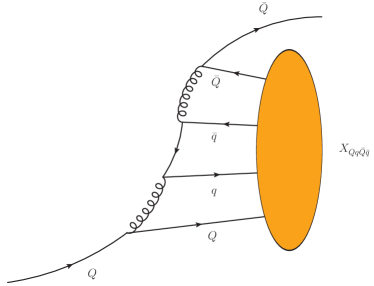
Figure 2: Leading diagram for the fragmentation of a heavy quark $Q$ into a $X_{Qq\bar{Q}\bar{q}}$ tetraquark. The orange blob portrays the nonperturbative hadronization of the $(Qq\bar{Q}\bar{q})$ system into the bound state. The diagram was made by using JaxoDraw 2.0 [272].

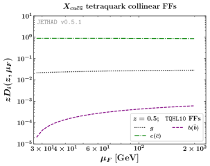
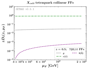
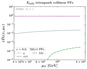
Figure 3: Dependence on $\mu_{F}$ of the four TQHL1.0 collinear FF sets describing $X_{Qq\bar{Q}\bar{q}}$ tetraquark formation at $z\simeq\langle z\rangle=0.5$.

4 Exotic tetraquarks at the HL-LHC with Jethad

All the predictions given in this review were obtained by making use of Jethad, a hybrid and multimodular interface which combines both Python- and Fortran-based modules. Jethad is designed for the computation, management, and processing of physical distributions defined within various formalisms [79, 80, 81]. In particular, numeric calculations of differential distributions were carried out via some of the Fortran 2008 modular routines within Jethad, whereas the native Python 3.0 analyzer served as a reference tool for final elaborations.

Section 4.1 provides an overview of the key features of the current version of Jethad technology (v0.5.1), which is not yet public. Further details on our error analysis are outlined in Section 4.2. Information regarding final-state kinematic cuts enforced can be found in Section 4.3. Numeric results and discussions on rapidity-interval and transverse-momentum rates are presented in Sections 4.4 and 4.5, respectively.

4.1 The Jethad v0.5.1 multimodular interface

The beginning of the Jethad project traces back to late 2017, driven by the need for accurate predictions of semi-hard hadron [183, 185] and jet [176, 178, 202] sensitive final states at the LHC. Phenomenological studies of such reactions, proposed as probe channels for the high-energy resummation in QCD, necessitated the establishment of a reference numeric technology devoted to the computation and analysis of high-energy related distributions.

Jethad v0.2.7 was the first named version and it played a key role in providing us with a pioneering BFKL-versus-DGLAP analysis in the context of semi-inclusive hadron-plus-jet emissions at the LHC [79]. Subsequent versions introduced new features, such as selecting forward heavy-quark pair observables (v0.3.0 [164]), enabling studies on Higgs emissions and transverse-momentum distributions (v0.4.2 [83]), and integrating the Python analyzer with the Fortran core supermodule (v0.4.3 [84]).

Advancements went on with the possibility to make analyses on heavy-flavored hadrons via VFNS FFs at NLO (v0.4.4 [213]). The Δϒναμις (DYnamis) work package, dedicated to the forward Drell–Yan dilepton reaction [242], became part of Jethad in v0.4.5. The integration with the Leptonic-Exclusive-Amplitudes (LExA) modular code allowed Jethad to explore the proton content at low-$x$ through small-$x$ TMD densities in v0.4.6 [231].

Version v0.4.7 [85] introduced quarkonium-sensitive reactions from NRQCD leading-twist fragmentation. The latest features in v0.5.0 [81] and v0.5.1 [221] encompass an enhanced system for MHOU-related studies, an expanded list of observables with a focus on singly- and doubly-differential transverse-momentum production rates [182, 206, 221], and support for matching procedures with collinear factorization [266, 267, 268, 269, 271].

From the fundamental core to service modules and routines, Jethad has been designed to dynamically achieve high levels of computational performance. The multidimensional integrators within Jethad leverage extensive parallel computing to actively choose the most suitable integration algorithm based on the shape of the integrand.

Any reaction analyzable with Jethad can be dynamically selected through an intuitive, structure based smart-management interface. Physical final-state particles are represented by object prototypes within this interface, where particle objects encapsulate all pertinent information about their physical counterparts, ranging from mass and charge to kinematic ranges and rapidity tags. These particle objects are initially loaded from a master database using a dedicated particle generation routine, and custom particle generation is also supported. Then, these objects are cloned into a final-state vector and injected from the integrand routine to the corresponding, process-specific module by a dedicated controller.

The flexibility in generating the physical final states is accompanied by a range of options for selecting the initial state. A unique particle-ascendancy structure attribute enables Jethad to rapidly learn whether a object is hadroproduced, electroproduced, photoproduced, etc. This dynamic feature ensures that only relevant modules are initialized, optimizing computing-time efficiency.

Jethad is structured as an object-based interface that is entirely independent of the specific reaction under investigation. While originally inspired by high-energy QCD and TMD factorization phenomenology, the code’s design allows for easy encoding of different approaches by simply implementing novel, dedicated (super)modules. These can be straightforwardly linked to the core structure of the code by means of a natively-equipped point-to-routine system, making Jethad a versatile, particle-physics oriented environment.

Having in mind providing the Scientific Community with a standard computation technology tailored for the management of diverse processes (described by distinct formalisms), we envision releasing the first public version of Jethad in the medium-term future.

4.2 Error analysis

A commonly employed methodology for gauging the impact of MHOUs involves evaluating the sensitivity of our observables to variations of the renormalization scale and the factorization one around their natural values.

It is widely recognized that MHOUs strongly contribute to the overall uncertainty [80]. To assess their weight, we vary $\mu_{R}$ and $\mu_{F}$ simultaneously around $\mu_{N}/2$ and $2\mu_{N}$, with the $C_{\mu}$ parameter in the figures of Sections 4.4 and 4.5 given as $C_{\mu}\equiv\mu_{F}/\mu_{N}=\mu_{R}/\mu_{N}$.

Another potential source of uncertainty lies in proton PDFs. Recent analyses on high-energy production rates indicate that choosing different PDF parametrizations and members within the same set has a minimal effect [202, 79, 214, 80]. Thus, our observables will be calculated by considering just the central member of the NNPDF4.0 parametrization.

Additional uncertainties may arise from a collinear improvement of the NLO kernel, involving the inclusion of renormalization-group (RG) terms to make the BFKL equation compatible with the DGLAP one in the collinear limit, or from changes in the renormalization scheme [339, 340, 341, 342, 343, 344, 345]. The impact of collinear-improvement techniques on semi-hard rapidity-differential rates is found to be contained within error bands produced by MHOUs [80].

Then, the $\overline{\rm MS}$ [273] to MOM [346, 347] renormalization-scheme transition was estimated in Ref. [80] and leads to systematically higher MOM results for rapidity distributions. However, these results remain within the MHOUs bands. We note, however, that a proper MOM analysis should be based on MOM-evolved PDFs and FFs, which are not currently available.

To derive uncertainty bands for our distributions, we combine MHOUs with the numerical errors generated by multidimensional integration (see Section 4.3). The latter is consistently maintained below $1\%$ thanks to the Jethad integrators.

4.3 Final-state kinematic cuts

The first observable matter of our investigation is the rapidity-interval rate, also known as $\Delta Y$-distribution. It is given by the ${\cal C}_{0}$ azimuthal coefficient, defined in Section 2.2, integrated over transverse momenta and rapidities of the two outgoing particles, while their rapidity distance, $\Delta Y$, is kept fixed. We write

$$\frac{{\rm d}\sigma(\Delta Y,s)}{{\rm d}\Delta Y}=\int_{|\bm{\kappa}_{1}|^{\rm min}}^{|\bm{\kappa}_{1}|^{\rm max}}\!\!{\rm d}|\bm{\kappa}_{1}|\int_{|\bm{\kappa}_{2}|^{\rm min}}^{|\bm{\kappa}_{2}|^{\rm max}}\!\!{\rm d}|\bm{\kappa}_{2}|\int_{\max\,(y_{1}^{\rm min},\,y_{2}^{\rm min}+\Delta Y)}^{\min\,(y_{1}^{\rm max},\,y_{2}^{\rm max}+\Delta Y)}{\rm d}y_{1}\,\,{\cal C}_{0}^{\rm[accuracy]}\left(|\bm{\kappa}_{1}|,|\bm{\kappa}_{2}|,y_{1},y_{2},s\right)\Bigm{\lvert}_{\Delta Y\;\equiv\;y_{1}-y_{2}}\;,$$ (20)

the ‘${\rm[accuracy]}$’ superscript of ${\cal C}_{0}$ inclusively denoting ${\rm NLL/NLO^{+}}$, ${\rm HE}\mbox{-}{\rm NLO^{+}}$, or ${\rm LL/LO}$. The $\delta(\Delta Y-y_{1}+y_{2})$ function enforces the fixed-$\Delta Y$ condition and thus removes one of the two rapidity integration: $y_{2}$ in our case. The transverse momentum of the forward hadron (always a tetraquark) lie in the range $30<|\bm{\kappa}_{1}|/{\rm GeV}<120$, whereas the one of the backward object (a singly heavy-flavored hadron or a light-flavored jet) stays in the range $50<|\bm{\kappa}_{1}|/{\rm GeV}<120$.

These tailoring cuts allow the VFNS-based fragmentation approach to be valid, since energy scales are higher than thresholds for the DGLAP evolution of heavy quarks. Furthermore, asymmetric transverse-momentum windows permit to better disengage the pure resummation dynamics from the fixed-order background [176, 177, 79]. They also suppress large Sudakov logarithms arising from (quasi) back-to-back emissions which are systematically missed by BFKL [348, 349, 350, 351, 352, 353]. Finally, they dampen instabilities encoded in higher-order contributions [354, 355] and drastically reduce energy-momentum-conservation breaking effects [356]. Rapidity configurations are the typical ones of current LHC studies. In particular, hadrons are tagged only in the barrel calorimeter [357], say $|y_{1,2}|<2.4$, while jets can be also detected by endcap detector [358], say $|y_{2}|<4.7$.

The second observable considered is the $|\bm{\kappa}_{1}|$-rate given by ${\cal C}_{0}$ coefficient, integrated over rapidities while $\Delta Y$ is kept fixed, and integrated over $|\bm{\kappa}_{2}|$ but not over $|\bm{\kappa}_{1}|$

$$\frac{{\rm d}\sigma(|\bm{\kappa}_{1}|,\Delta Y,s)}{{\rm d}|\bm{\kappa}_{1}|{\rm d}\Delta Y}=\int_{|\bm{\kappa}_{1}|^{\rm min}}^{|\bm{\kappa}_{1}|^{\rm max}}\!\!{\rm d}|\bm{\kappa}_{1}|\int_{\max\,(y_{1}^{\rm min},\,y_{2}^{\rm min}+\Delta Y)}^{\min\,(y_{1}^{\rm max},\,y_{2}^{\rm max}+\Delta Y)}{\rm d}y_{1}\,\,{\cal C}_{0}^{\rm[accuracy]}\left(|\bm{\kappa}_{1}|,|\bm{\kappa}_{2}|,y_{1},y_{2},s\right)\Bigm{\lvert}_{\Delta Y\;\equiv\;y_{1}-y_{2}}\;.$$ (21)

The last distribution considered is the $(|\bm{\kappa}_{1}|=|\bm{\kappa}_{2}|)$-rate, namely the ${\cal C}_{0}$ coefficient, integrated over rapidities while $\Delta Y$ is kept fixed, differential in $|\bm{\kappa}_{1}|$ and $|\bm{\kappa}_{2}|$, but with the $|\bm{\kappa}_{1}|=|\bm{\kappa}_{2}|$ constraint enforced

$$\frac{{\rm d}\sigma(|\bm{\kappa}_{1}|=|\bm{\kappa}_{2}|,\Delta Y,s)}{{\rm d}|\bm{\kappa}_{1}|{\rm d}|\bm{\kappa}_{2}|{\rm d}\Delta Y}=\int_{\max\,(y_{1}^{\rm min},\,y_{2}^{\rm min}+\Delta Y)}^{\min\,(y_{1}^{\rm max},\,y_{2}^{\rm max}+\Delta Y)}{\rm d}y_{1}\,\,{\cal C}_{0}^{\rm[accuracy]}\left(|\bm{\kappa}_{1}|,|\bm{\kappa}_{2}|\equiv|\bm{\kappa}_{1}|,y_{1},y_{2},s\right)\Bigm{\lvert}_{\Delta Y\;\equiv\;y_{1}-y_{2}}\;.$$ (22)

For both the $(|\bm{\kappa}_{1}|$- and the $(|\bm{\kappa}_{1}|=|\bm{\kappa}_{2}|)$-rate rapidities stay in the same range which the $\Delta Y$-distribution it tailored on, while the nonintegrated transverse momenta span from 10 to 120 GeV. To study configurations that align well with prospective HL-LHC data, we average our predictions on transverse-momentum bins set at a constant width of 10 GeV. Then, $\Delta Y$ will be integrated in a characteristic forward bin, say $3<\Delta Y<4.5$ for the tetraquark-plus-hadron case, and $4<\Delta Y<6$ for the tetraquark-plus-jet one.

4.4 Rapidity-interval rates

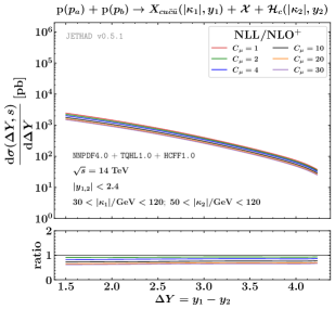
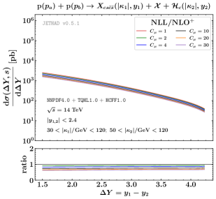
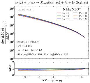
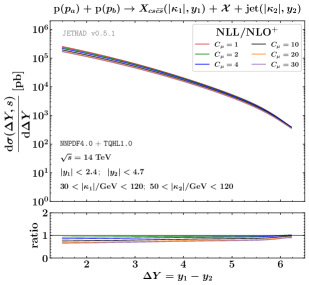
Figure 4: ${\rm NLL/NLO^{+}}$ versus ${\rm HE}\mbox{-}{\rm NLO^{+}}$ $\Delta Y$-rates for $X_{cq\bar{c}\bar{q}}+{\cal H}_{Q}$ (upper) and $X_{cq\bar{c}\bar{q}}+{\rm jet}$ (lower) reactions at 14 TeV LHC. An extended study of MHOUs in the range $1<C_{\mu}<30$ is illustrated.

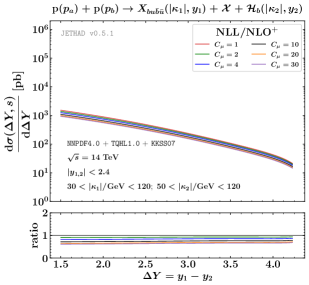
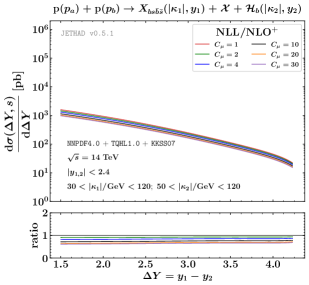
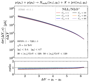
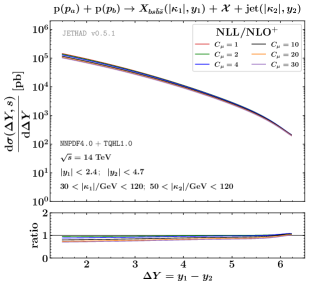
Figure 5: ${\rm NLL/NLO^{+}}$ versus ${\rm HE}\mbox{-}{\rm NLO^{+}}$ $\Delta Y$-rates for $X_{bq\bar{b}\bar{q}}+{\cal H}_{Q}$ (upper) and $X_{bq\bar{b}\bar{q}}+{\rm jet}$ (lower) reactions at 14 TeV LHC. An extended study of MHOUs in the range $1<C_{\mu}<30$ is illustrated.

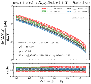
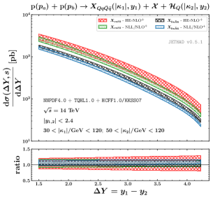
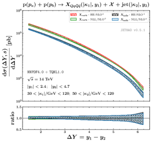
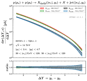
Figure 6: ${\rm NLL/NLO^{+}}$ versus ${\rm HE}\mbox{-}{\rm NLO^{+}}$ $\Delta Y$-rates for $X_{Qq\bar{Q}\bar{q}}+{\cal H}_{Q}$ (upper) and $X_{Qq\bar{Q}\bar{q}}+{\rm jet}$ (lower) reactions at 14 TeV LHC. Uncertainty bands are for the combined effect of MHOUs and errors on numeric integrations.

In this Section we present predictions for the rapidity-interval distribution for our reference processes (see Fig. 1). The main analysis depicted in Figs. 4 and 5 entails an examination of the observable across a wide spectrum. It is achieved through a progressive variation of factorization and renormalization scales, which spans a broad window, regulated by the parameter $C_{\mu}$ introduced in Section 4.2 and ranging from $1$ to $30$. This approach expands upon the conventional MHOU scan, which typically operates within the range $1/2<C_{\mu}<2$.

Left (right) plots of Fig. 4 contain ${\rm NLL/NLO^{+}}$ results for $X_{cu\bar{c}\bar{u}}$ ($X_{cs\bar{c}\bar{s}}$) production channels, whereas left (right) plots of Fig. 5 embody predictions for $X_{bu\bar{b}\bar{u}}$ ($X_{bs\bar{b}\bar{s}}$) corresponding ones. In all cases, upper (lower) plots are for tetraquark-plus-hadron (tetraquark-plus-jet) reactions. Ancillary panels below the primary ones display normalized distributions, obtained by dividing each distribution by its central value computed at $C_{\mu}=1$.

The general outcome from all eight examined final states is a minimal sensitivity to variations in $C_{\mu}$ across the entire range of $\Delta Y$ values explored in our analysis. This observation underscores the significant stabilizing mechanism embedded within our TQHL1.0 functions.

Results of Fig. 6 are for rapidity-interval distributions with a standard MHOU analysis in the range range $1/2<C_{\mu}<2$. The overall decreasing pattern with $\Delta Y$ of our $\Delta Y$-rates results from the interplay of two contrasting tendencies: while BFKL partonic cross sections increase with $\Delta Y$ and subsequently with energy, their convolution with collinear PDFs and FFs in the impact factors markedly restrains this escalation. Ancillary panels below primary plots in Fig. 6 underscore the stabilizing power of our TQHL1.0 FFs, with the ${\rm NLL/NLO^{+}}$ uncertainty bands consistently staying within the ${\rm LL/LO}$ ones for all channels.

We mention a pertinent aspect that extends the topic beyond the scope of this review, but still deserves a discussion. We refer to the influence of MPIs on differential distributions as the final-state rapidity distance $\Delta Y$ increase. Particularly noteworthy is the effect of the DPS. A recent analysis quantifies DPS corrections to Mueller–Navelet jets, potentially impacting $\Delta Y$-distributions at high center-of-mass energies and moderate transverse momenta [175].

Concerning quarkonia, studies of final states such as double $J/\psi$ [359, 360], $J/\psi$ plus $\Upsilon$ [360], $J/\psi$ plus electroweak-boson [361, 362], and triple $J/\psi$ [363, 364], have indicated the presence potentially large DPS contributions. Thus, the search for MPI signatures also in tetraquark-sensitive final states represents an important and promising avenue for future research.

4.5 Transverse-momentum rates

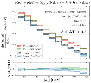
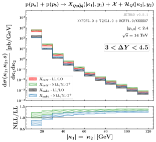
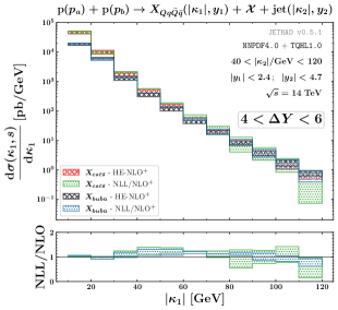
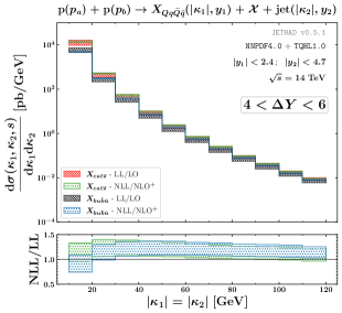
Figure 7: ${\rm NLL/NLO^{+}}$ transverse-momentum rates for $X_{Qq\bar{Q}\bar{q}}+{\cal H}_{Q}$ (upper) and $X_{Qq\bar{Q}\bar{q}}+{\rm jet}$ (lower) reactions at 14 TeV LHC. Uncertainty bands are for the combined effect of MHOUs and errors on numeric integrations.

The first transverse-momentum distribution matter of our investigation is the $|\bm{\kappa}_{1}|$-rate. This observable serves as a common basis whereby exploring potential links between our hybrid factorization and alternative formalisms. By varying $|\vec{\kappa}_{1}|$ within a wide range, we can delve into a broad kinematic domain, where alternative resummation techniques may become pertinent and necessary.

In scenarios where transverse momenta are high or widely separated, the magnitude of DGLAP-like logarithms and threshold contaminations increases, rendering a pure high-energy approach inadequate [365, 366, 367, 368, 369, 370, 371, 372, 373, 374, 375, 376, 377, 378, 379, 380, 381, 382]. Additionally, in the very-low transverse-momentum regime, enhanced $|\vec{\kappa}_{1}|$-logarithms, which are not accounted for by BFKL, become significant. Moreover, effects like diffusion patterns grow to a point where they impede the convergence of high-energy resummation [383, 384, 385].

In these kinematic corners, an all-order transverse-momentum (TM) resummation is necessary [386, 387, 388, 389, 390, 391, 392, 393]. TM-resummed distributions have been explored extensively in various processes, including photon [394, 395, 396, 397], Higgs [398], and $W$-boson pair production, as well as in final states involving bosons and jets. Recent studies have provided third-order fiducial predictions for Drell–Yan and Higgs emissions, incorporating TM resummation [399, 400, 401, 402, 403, 404, 400, 405]. Furthermore, when the transverse momenta of detected particles result in nearly back-to-back configurations, Sudakov-type logarithms emerge, requiring additional resummation techniques [406, 348, 349, 350, 351].

Left panels of Fig. 7 carry information about $|\bm{\kappa}_{1}|$-rates for tetraquark-plus-hadron (upper) and tetraquark-plus-jet (right) channels with their within ${\rm NLL/NLO^{+}}$ and ${\rm HE}\mbox{-}{\rm NLO^{+}}$ accuracies. Here, for the sake of brevity, we consider just the $X_{cs\bar{c}\bar{s}}$ and $X_{bu\bar{b}\bar{u}}$ channels, namely the ones complementary to our first study presented in Ref. [88]. Overall, we observe a falloff with increasing $|\bm{\kappa}_{1}|$ across the distributions. Notably, the results remain remarkably stable MHOU studies, with error bands generally confined within a 30% width, except for the initial and final two bins.

In the tetraquark-plus-hadron scenario, the NLL-resummed distribution initially appears smaller than its fixed-order counterpart in the first bin, subsequently reaching a comparable magnitude and exhibiting a slight upward trend with $|\bm{\kappa}_{1}|$. Conversely, in the case of hadron-plus-jet events, the resummation leads to a visible rise with $|\bm{\kappa}_{1}|$, reaching up to a 50% increase. However, larger uncertainties in the final two bins indicate a loss of stability for BFKL due to threshold contaminations. Notably, these uncertainties are less pronounced when detecting a bottomed tetraquark, aligning with recent findings suggesting that VFNS FFs for bottom-flavored hadrons offer greater stabilizing effects compared to their charm-flavored counterparts [214].

On the other hand, the initial bin may be susceptible to instabilities arising from energy scales nearing thresholds for DGLAP evolution dictated by heavy-quark masses. This could explain the downturn observed in the $X_{bu\bar{b}\bar{u}}$ NLL cross section with respect to the $X_{cs\bar{c}\bar{s}}$ one in the left upper plot, which could potentially stem from instabilities associated with values of $\mu_{F}$ approaching the bottom mass.

The final observable under investigation is a doubly differential distribution in both $|\bm{\kappa}_{1}|$ and $|\bm{\kappa}_{2}|$. As the separation between the two transverse momenta increases, additional kinematic regions adjacent to the BFKL regime become accessible (as observed in recent analyses on ${\cal H}_{b}$ hadrons [214] and $\Xi$ baryons [206]). A joint resummation of transverse-momentum logarithms for two-particle distributions was initially achieved in the context of Higgs-plus-jet hadroproduction [407] through the RadISH momentum-space method [403]. Here we make use of a complementary configuration by setting $|\bm{\kappa}_{1}|\equiv|\bm{\kappa}_{2}|$ and spanning them from 10 to 120 GeV, while maintaining the same rapidity bins as before. This choice permits to examine in deep the strict BFKL regime, thus easing a precise determination of the impact of higher-order corrections.

In the right plots of Fig. 7 we present ${\rm NLL/NLO^{+}}$ distributions for both the tetraquark-plus-hadron (upper) and hadron-plus-jet (lower) channel, juxtaposed with their ${\rm LL/LO}$ limits. To provide further insight, we magnify the NLL to LL ratio in ancillary plots. With the exception of the initial bin, where $X_{bu\bar{b}\bar{u}}$ cross sections are affected by instabilities due to their proximity to thresholds, NLL corrections in the upper plot exhibit a moderate increase with transverse momentum, plateauing at around +30%. Conversely, NLL corrections in the lower plot consistently augment LL results by approximately +30% across the entire spectrum. This dichotomy arises from the positive sign of NLO hadron impact-factor corrections owing to large values of the $(gg)$ channel [185], while NLO jet corrections are generally negative [171, 173, 176, 182].

5 Final remarks

We made use of the hybrid high-energy and collinear factorization framework at ${\rm NLL/NLO^{+}}$ to conduct a comprehensive study of the inclusive hadroproduction of four different species of exotic heavy-light tetraquark at high energies. We described the formation of tetraquark states by means of the single-parton collinear-fragmentation mechanism at leading twist, which holds validity in the large transverse-momentum regime pertinent to our analysis.

To this end, we developed first tetraquark collinear NLO FF sets, named TQHL1.0 functions. They were constructed by DGLAP-evolving a SNAJ-inspired model input for the heavy-quark channel [89, 90, 91, 92]. The interconnection between high-energy resummation and the fragmentation mechanism played a crucial role in our analysis.

Notably, we observed that the distinct behavior of the gluon-to-tetraquark fragmentation channel acts as a robust stabilizer of the hybrid factorization scheme under NLL corrections and scale variations. This enabled us to achieve a remarkable level of accuracy in describing our observables at the natural scales provided by kinematics. Natural stability, revealed as a general property across various heavy-flavored species considered thus far, including single heavy-flavored hadrons [213, 214, 80, 219], vector quarkonia [85, 81], and charmed $B$ mesons [218, 221]), was now found also in the case of $X_{Qq\bar{Q}\bar{q}}$ states as well.

As for future tetraquark studies within high-energy QCD, a step forward would come out from linking our program with NLO investigations of single-forward or nearly back-to-back semi-inclusive emissions within the framework of gluon saturation (see, for instance, Refs. [408, 409, 410, 411, 412, 413, 414, 415, 416, 417, 418, 419, 420] and references therein). In these analyses, the influence of soft-gluon radiation on angular asymmetries in dijet or dihadron production was addressed (see Refs. [352, 353, 421, 422, 423, 424]).

NLO saturation allows us to access the (un)polarized gluon content of protons and nucleons at small-$x$ [425, 426, 427, 428, 429, 430]. Authors of Refs. [431, 432, 433, 434, 435] explore heavy-hadron emissions in proton-proton and proton-nucleus collisions by incorporating small-$x$ effects. Future investigations will explore the intersection between our approach to tetraquarks production via the ${\rm NLL/NLO^{+}}$ hybrid factorization and higher-order calculations for NLO saturation in exclusive emissions of heavy particles [436, 437].

A milestone in deepening our understanding of tetraquark fragmentation will rely upon comparing predictions from our TQHL1.0 FFs with ones based on functions extracted from global data. Along this direction, artificial-intelligence techniques already adapted to address the collinear fragmentation of lighter-hadron species [438, 439, 440, 441, 442, 443, 444, 445] will be an asset.

As a prospect, we plan to extend to explore heavy-light tetraquark production through other resummations, as well as by using different inputs for the initial-scale fragmentation and through exclusive reactions. Promising avenues to be investigated via the fragmentation approximation include emissions of fully-charmed tetraquarks [446, 447, 448, 449] and pentaquarks [450, 451, 452].

Until recently, the $X(3872)$ was the sole exotic state observed in prompt proton collisions. However, the discovery of fully-charmed structures [453] and the $T_{cc}$ [454, 455] brought novelty to the exotic-physics panorama. Extending our fragmentation approach to these states should be feasible and could offer valuable insights. Additionally, it could be applied to investigate the $Z_{c}(3900)$, which has not yet been observed promptly [456].

While further analyses are required from both the theoretical and phenomenological perspectives, we believe that the present study can contribute to open new windows of discovery. This gives us an intriguing opportunity to gain deeper insights into the true nature of exotic matter, which can be explored at the HL-LHC and at future colliders [457, 458, 459, 460, 461, 462, 463, 464, 465, 466, 467, 468, 469, 470, 471, 472, 473, 474, 475, 476, 477, 478, 479, 480, 481, 482, 483, 484].

Data availability

The four grids for the TQHL1.0 FF determinations

• NLO, $X_{bu\bar{b}\bar{u}}$ :  TQHL10_Xbu_nlo;

• NLO, $X_{cu\bar{c}\bar{u}}$ :  TQHL10_Xcu_nlo;

• NLO, $X_{bs\bar{b}\bar{s}}$ :  TQHL10_Xbs_nlo;

• NLO, $X_{cs\bar{c}\bar{s}}$ :  TQHL10_Xcs_nlo,

can be publicly accessed from the following url: https://github.com/FGCeliberto/Collinear_FFs/.

Appendix A: NLO correction for the heavy-hadron singly off-shell emission function

The analytic expression for the NLO correction to the forward heavy-hadron singly off-shell emission function reads [148]

$$\hat{\cal F}_{h}(n,\nu,|\bm{\kappa}_{h}|,x_{h})=\frac{1}{\pi}\sqrt{\frac{C_{F}}{C_{A}}}\left(|\bm{\kappa}_{h}|^{2}\right)^{i\nu-\frac{1}{2}}\int_{x_{h}}^{1}\frac{{\rm d}x}{x}\int_{\frac{x_{h}}{x}}^{1}\frac{{\rm d}\eta}{\eta}\left(\frac{x\eta}{x_{h}}\right)^{2i\nu-1}$$ (23)

$$\times\,\left[\frac{C_{A}}{C_{F}}f_{g}(x)D_{g}^{h}\left(\frac{x_{h}}{x\eta}\right){\cal C}_{gg}\left(x,\eta\right)+\sum_{i=q\bar{q}}f_{i}(x)D_{i}^{h}\left(\frac{x_{h}}{x\eta}\right){\cal C}_{qq}\left(x,\eta\right)\right.$$

$$\times\,\left.D_{g}^{h}\left(\frac{x_{h}}{x\eta}\right)\sum_{i=q\bar{q}}f_{i}(x){\cal C}_{qg}\left(x,\eta\right)+\frac{C_{A}}{C_{F}}f_{g}(x)\sum_{i=q\bar{q}}D_{i}^{h}\left(\frac{x_{h}}{x\eta}\right){\cal C}_{gq}\left(x,\eta\right)\right]\,,$$

with the ${\cal C}_{ij}$ partonic coefficients being

$${\cal C}_{gg}\left(x,\eta\right)=P_{gg}(\eta)\left(1+\eta^{-2\gamma}\right)\ln\left(\frac{|\bm{\kappa}_{h}|^{2}x^{2}\eta^{2}}{\mu_{F}^{2}x_{h}^{2}}\right)-\frac{\beta_{0}}{2}\ln\left(\frac{|\bm{\kappa}_{h}|^{2}x^{2}\eta^{2}}{\mu^{2}_{R}x_{h}^{2}}\right)$$ (24)

$$+\,\delta(1-\eta)\left[C_{A}\ln\left(\frac{s_{0}\,x^{2}}{|\bm{\kappa}_{h}|^{2}\,x_{h}^{2}}\right)\chi(n,\gamma)-C_{A}\left(\frac{67}{18}-\frac{\pi^{2}}{2}\right)+\frac{5}{9}n_{f}\right.$$

$$\left.+\frac{C_{A}}{2}\left(\psi^{\prime}\left(1+\gamma+\frac{n}{2}\right)-\psi^{\prime}\left(\frac{n}{2}-\gamma\right)-\chi^{2}(n,\gamma)\right)\right]+\,C_{A}\left(\frac{1}{\eta}+\frac{1}{(1-\eta)_{+}}-2+\eta\bar{\eta}\right)$$

$$\times\,\left(\chi(n,\gamma)(1+\eta^{-2\gamma})-2(1+2\eta^{-2\gamma})\ln\eta+\frac{\bar{\eta}^{2}}{\eta^{2}}{\cal I}_{2}\right)$$

$$+\,2\,C_{A}(1+\eta^{-2\gamma})\left(\left(\frac{1}{\eta}-2+\eta\bar{\eta}\right)\ln\bar{\eta}+\left(\frac{\ln(1-\eta)}{1-\eta}\right)_{+}\right)\ ,$$

$${\cal C}_{gq}\left(x,\eta\right)=P_{qg}(\eta)\left(\frac{C_{F}}{C_{A}}+\eta^{-2\gamma}\right)\ln\left(\frac{|\bm{\kappa}_{h}|^{2}x^{2}\eta^{2}}{\mu_{F}^{2}x_{h}^{2}}\right)$$ (25)

$$+\,2\,\eta\bar{\eta}\,T_{R}\,\left(\frac{C_{F}}{C_{A}}+\eta^{-2\gamma}\right)+\,P_{qg}(\eta)\,\left(\frac{C_{F}}{C_{A}}\,\chi(n,\gamma)+2\eta^{-2\gamma}\,\ln\frac{\bar{\eta}}{\eta}+\frac{\bar{\eta}}{\eta}{\cal I}_{3}\right)\ ,$$

$${\cal C}_{qg}\left(x,\eta\right)=P_{gq}(\eta)\left(\frac{C_{A}}{C_{F}}+\eta^{-2\gamma}\right)\ln\left(\frac{|\bm{\kappa}_{h}|^{2}x^{2}\eta^{2}}{\mu_{F}^{2}x_{h}^{2}}\right)$$ (26)

$$+\eta\left(C_{F}\eta^{-2\gamma}+C_{A}\right)+\,\frac{1+\bar{\eta}^{2}}{\eta}\left[C_{F}\eta^{-2\gamma}(\chi(n,\gamma)-2\ln\eta)+2C_{A}\ln\frac{\bar{\eta}}{\eta}+\frac{\bar{\eta}}{\eta}{\cal I}_{1}\right]\ ,$$

and

$${\cal C}_{qq}\left(x,\eta\right)=P_{qq}(\eta)\left(1+\eta^{-2\gamma}\right)\ln\left(\frac{|\bm{\kappa}_{h}|^{2}x^{2}\eta^{2}}{\mu_{F}^{2}x_{h}^{2}}\right)-\frac{\beta_{0}}{2}\ln\left(\frac{|\bm{\kappa}_{h}|^{2}x^{2}\eta^{2}}{\mu^{2}_{R}x_{h}^{2}}\right)$$ (27)

$$+\,\delta(1-\eta)\left[C_{A}\ln\left(\frac{s_{0}\,x_{h}^{2}}{|\bm{\kappa}_{h}|^{2}\,x^{2}}\right)\chi(n,\gamma)+C_{A}\left(\frac{85}{18}+\frac{\pi^{2}}{2}\right)-\frac{5}{9}n_{f}-8\,C_{F}\right.$$

$$\left.+\frac{C_{A}}{2}\left(\psi^{\prime}\left(1+\gamma+\frac{n}{2}\right)-\psi^{\prime}\left(\frac{n}{2}-\gamma\right)-\chi^{2}(n,\gamma)\right)\right]+\,C_{F}\,\bar{\eta}\,(1+\eta^{-2\gamma})$$

$$+\left(1+\eta^{2}\right)\left[C_{A}(1+\eta^{-2\gamma})\frac{\chi(n,\gamma)}{2(1-\eta)_{+}}+\left(C_{A}-2\,C_{F}(1+\eta^{-2\gamma})\right)\frac{\ln\eta}{1-\eta}\right]$$

$$+\,\left(C_{F}-\frac{C_{A}}{2}\right)\left(1+\eta^{2}\right)\left[2(1+\eta^{-2\gamma})\left(\frac{\ln(1-\eta)}{1-\eta}\right)_{+}+\frac{\bar{\eta}}{\eta^{2}}{\cal I}_{2}\right]\;,$$

The $s_{0}$ scale is a BFKL-typical energy-normalization parameter, usually set to $s_{0}=\mu_{C}$. Furthermore, one has $\bar{\eta}\equiv 1-\eta$ and $\gamma\equiv-\frac{1}{2}+i\nu$. The LO DGLAP $P_{ij}(\eta)$ splitting functions read

$$P_{gq}(z) = C_{F}\frac{1+(1-z)^{2}}{z}\;,$$ (28)

$$P_{qg}(z) = T_{R}\left[z^{2}+(1-z)^{2}\right]\;,$$

$$P_{qq}(z) = C_{F}\left(\frac{1+z^{2}}{1-z}\right)_{+}=C_{F}\left[\frac{1+z^{2}}{(1-z)_{+}}+{3\over 2}\delta(1-z)\right]\;,$$

$$P_{gg}(z) = 2C_{A}\left[\frac{1}{(1-z)_{+}}+\frac{1}{z}-2+z(1-z)\right]+\left({11\over 6}C_{A}-\frac{n_{f}}{3}\right)\delta(1-z)\;,$$

while the ${\cal I}_{2,1,3}$ functions are

$${\cal I}_{2}=\frac{\eta^{2}}{\bar{\eta}^{2}}\left[\eta\left(\frac{{}_{2}F_{1}(1,1+\gamma-\frac{n}{2},2+\gamma-\frac{n}{2},\eta)}{\frac{n}{2}-\gamma-1}-\frac{{}_{2}F_{1}(1,1+\gamma+\frac{n}{2},2+\gamma+\frac{n}{2},\eta)}{\frac{n}{2}+\gamma+1}\right)\right.$$ (29)

$$\left.+\eta^{-2\gamma}\left(\frac{{}_{2}F_{1}(1,-\gamma-\frac{n}{2},1-\gamma-\frac{n}{2},\eta)}{\frac{n}{2}+\gamma}-\frac{{}_{2}F_{1}(1,-\gamma+\frac{n}{2},1-\gamma+\frac{n}{2},\eta)}{\frac{n}{2}-\gamma}\right)\right.$$

$$\left.+\left(1+\eta^{-2\gamma}\right)\left(\chi(n,\gamma)-2\ln\bar{\eta}\right)+2\ln{\eta}\right]\;,$$

$${\cal I}_{1}=\frac{\bar{\eta}}{2\eta}{\cal I}_{2}+\frac{\eta}{\bar{\eta}}\left[\ln\eta+\frac{1-\eta^{-2\gamma}}{2}\left(\chi(n,\gamma)-2\ln\bar{\eta}\right)\right]\;,$$ (30)

and

$${\cal I}_{3}=\frac{\bar{\eta}}{2\eta}{\cal I}_{2}-\frac{\eta}{\bar{\eta}}\left[\ln\eta+\frac{1-\eta^{-2\gamma}}{2}\left(\chi(n,\gamma)-2\ln\bar{\eta}\right)\right]\;.$$ (31)

Moreover, ${}_{2}F_{1}$ stands for the Gauss hypergeometric function.

The plus prescription in Eqs. (24) and (27) is given by

$$\int^{1}_{\zeta}{\rm d}x\frac{f(x)}{(1-x)_{+}}=\int^{1}_{\zeta}{\rm d}x\frac{f(x)-f(1)}{(1-x)}-\int^{\zeta}_{0}{\rm d}x\frac{f(1)}{(1-x)}\;,$$ (32)

where $f(x)$ represents a regular-behaved generic function at $y=1$.

Appendix B: NLO correction for the light-jet singly off-shell emission function

The analytic expression for the NLO correction to the forward light-jet singly off-shell emission function within the small-cone algorithm reads [145, 147]

$$\hat{\cal F}_{J}(n,\nu,|\bm{\kappa}_{J}|,x_{J})=\frac{1}{\pi}\sqrt{\frac{C_{F}}{C_{A}}}\left(|\bm{\kappa}_{J}|^{2}\right)^{i\nu-1/2}\int^{1}_{x_{J}}\frac{{\rm d}\eta}{\eta}\eta^{-\bar{\alpha}_{s}(\mu_{R})\chi(n,\nu)}$$ (33)

$$\times\;\left\{\sum_{i=q,\bar{q}}f_{i}\left(\frac{x_{J}}{\eta}\right)\left[\left(P_{qq}(\eta)+\frac{C_{A}}{C_{F}}P_{gq}(\eta)\right)\ln\frac{|\bm{\kappa}_{J}|^{2}}{\mu_{F}^{2}}\right.\right.$$

$$-\;2\eta^{-2\gamma}\ln\frac{{\cal R}}{\max(\eta,\bar{\eta})}\,\left\{P_{qq}(\eta)+P_{gq}(\eta)\right\}-\frac{\beta_{0}}{2}\ln\frac{|\bm{\kappa}_{J}|^{2}}{\mu_{R}^{2}}\delta(1-\eta)$$

$$+\;C_{A}\delta(1-\eta)\left[\chi(n,\gamma)\ln\frac{s_{0}}{|\bm{\kappa}_{J}|^{2}}+\frac{85}{18}\right.$$

$$\left.+\;\frac{\pi^{2}}{2}+\frac{1}{2}\left(\psi^{\prime}\left(1+\gamma+\frac{n}{2}\right)-\psi^{\prime}\left(\frac{n}{2}-\gamma\right)-\chi^{2}(n,\gamma)\right)\right]$$

$$+\;(1+\eta^{2})\left\{C_{A}\left[\frac{(1+\eta^{-2\gamma})\,\chi(n,\gamma)}{2(1-\eta)_{+}}-\eta^{-2\gamma}\left(\frac{\ln(1-\eta)}{1-\eta}\right)_{+}\right]\right.$$

$$\left.+\;\left(C_{F}-\frac{C_{A}}{2}\right)\left[\frac{\bar{\eta}}{\eta^{2}}{\cal I}_{2}-\frac{2\ln\eta}{1-\eta}+2\left(\frac{\ln(1-\eta)}{1-\eta}\right)_{+}\right]\right\}$$

$$+\;\delta(1-\eta)\left(C_{F}\left(3\ln 2-\frac{\pi^{2}}{3}-\frac{9}{2}\right)-\frac{5n_{f}}{9}\right)+C_{A}\eta+C_{F}\bar{\eta}$$

$$\left.+\;\frac{1+\bar{\eta}^{2}}{\eta}\left(C_{A}\frac{\bar{\eta}}{\eta}{\cal I}_{1}+2C_{A}\ln\frac{\bar{\eta}}{\eta}+C_{F}\eta^{-2\gamma}(\chi(n,\gamma)-2\ln\bar{\eta})\right)\right]$$

$$+\;f_{g}\left(\frac{x_{J}}{\eta}\right)\frac{C_{A}}{C_{F}}\left[\left(P_{gg}(\eta)+2\,n_{f}\frac{C_{F}}{C_{A}}P_{qg}(\eta)\right)\ln\frac{|\bm{\kappa}_{J}|^{2}}{\mu_{F}^{2}}\right.$$

$$\left.-\;2\eta^{-2\gamma}\ln\frac{{\cal R}}{\max(\eta,\bar{\eta})}\left(P_{gg}(\eta)+2\,n_{f}P_{qg}(\eta)\right)-\frac{\beta_{0}}{2}\ln\frac{|\bm{\kappa}_{J}|^{2}}{4\mu_{R}^{2}}\delta(1-\eta)\right.$$

$$\left.+\;C_{A}\delta(1-\eta)\left(\chi(n,\gamma)\ln\frac{s_{0}}{|\bm{\kappa}_{J}|^{2}}+\frac{1}{12}+\frac{\pi^{2}}{6}\right.\right.$$

$$\left.+\;\frac{1}{2}\left[\psi^{\prime}\left(1+\gamma+\frac{n}{2}\right)-\psi^{\prime}\left(\frac{n}{2}-\gamma\right)-\chi^{2}(n,\gamma)\right]\right)$$

$$+\,2C_{A}(1-\eta^{-2\gamma})\left(\left(\frac{1}{\eta}-2+\eta\bar{\eta}\right)\ln\bar{\eta}+\frac{\ln(1-\eta)}{1-\eta}\right)$$

$$+\,C_{A}\,\left[\frac{1}{\eta}+\frac{1}{(1-\eta)_{+}}-2+\eta\bar{\eta}\right]\left((1+\eta^{-2\gamma})\chi(n,\gamma)-2\ln\eta+\frac{\bar{\eta}^{2}}{\eta^{2}}{\cal I}_{2}\right)$$

$$\left.\left.+\,n_{f}\left[\,2\eta\bar{\eta}\,\frac{C_{F}}{C_{A}}+(\eta^{2}+\bar{\eta}^{2})\left(\frac{C_{F}}{C_{A}}\chi(n,\gamma)+\frac{\bar{\eta}}{\eta}{\cal I}_{3}\right)-\frac{1}{12}\delta(1-\eta)\right]\right]\right\}\;,$$

with ${\cal R}$ denoting the jet-cone radius.

References

- [1] M. Gell-Mann, Symmetries of baryons and mesons, Phys. Rev. 125 (1962) 1067–1084. doi:10.1103/PhysRev.125.1067.
- [2] M. Gell-Mann, A Schematic Model of Baryons and Mesons, Phys. Lett. 8 (1964) 214–215. doi:10.1016/S0031-9163(64)92001-3.
- [3] G. Zweig, An SU(3) model for strong interaction symmetry and its breaking. Version 2, 1964, pp. 22–101.
- [4] H. Fritzsch, M. Gell-Mann, H. Leutwyler, Advantages of the Color Octet Gluon Picture, Phys. Lett. B 47 (1973) 365–368. doi:10.1016/0370-2693(73)90625-4.
- [5] R. D. Peccei, H. R. Quinn, CP Conservation in the Presence of Instantons, Phys. Rev. Lett. 38 (1977) 1440–1443. doi:10.1103/PhysRevLett.38.1440.
- [6] R. D. Peccei, H. R. Quinn, Constraints Imposed by CP Conservation in the Presence of Instantons, Phys. Rev. D 16 (1977) 1791–1797. doi:10.1103/PhysRevD.16.1791.
- [7] R. D. Peccei, The Strong CP problem and axions, Lect. Notes Phys. 741 (2008) 3–17. arXiv:hep-ph/0607268, doi:10.1007/978-3-540-73518-2_1.
- [8] L. D. Duffy, K. van Bibber, Axions as Dark Matter Particles, New J. Phys. 11 (2009) 105008. arXiv:0904.3346, doi:10.1088/1367-2630/11/10/105008.
- [9] L. Forestell, D. E. Morrissey, K. Sigurdson, Cosmological Bounds on Non-Abelian Dark Forces, Phys. Rev. D 97 (7) (2018) 075029. arXiv:1710.06447, doi:10.1103/PhysRevD.97.075029.
- [10] W.-C. Huang, M. Reichert, F. Sannino, Z.-W. Wang, Testing the dark SU(N) Yang-Mills theory confined landscape: From the lattice to gravitational waves, Phys. Rev. D 104 (3) (2021) 035005. arXiv:2012.11614, doi:10.1103/PhysRevD.104.035005.
- [11] L. McLerran, R. D. Pisarski, Phases of cold, dense quarks at large N(c), Nucl. Phys. A 796 (2007) 83–100. arXiv:0706.2191, doi:10.1016/j.nuclphysa.2007.08.013.
- [12] Y. Hidaka, L. D. McLerran, R. D. Pisarski, Baryons and the phase diagram for a large number of colors and flavors, Nucl. Phys. A 808 (2008) 117–123. arXiv:0803.0279, doi:10.1016/j.nuclphysa.2008.05.009.
- [13] L. McLerran, S. Reddy, Quarkyonic Matter and Neutron Stars, Phys. Rev. Lett. 122 (12) (2019) 122701. arXiv:1811.12503, doi:10.1103/PhysRevLett.122.122701.
- [14] W. Buchmuller, D. Wyler, Effective Lagrangian Analysis of New Interactions and Flavor Conservation, Nucl. Phys. B 268 (1986) 621–653. doi:10.1016/0550-3213(86)90262-2.
- [15] E. Witten, Baryons in the 1/n Expansion, Nucl. Phys. B 160 (1979) 57–115. doi:10.1016/0550-3213(79)90232-3.
- [16] J. J. Dudek, R. G. Edwards, M. J. Peardon, D. G. Richards, C. E. Thomas, Toward the excited meson spectrum of dynamical QCD, Phys. Rev. D 82 (2010) 034508. arXiv:1004.4930, doi:10.1103/PhysRevD.82.034508.
- [17] S. S. Afonin, The effect of higher dimensional QCD operators on the spectroscopy of bottom-up holographic models, Universe 7 (4) (2021) 102. arXiv:1905.13086, doi:10.3390/universe7040102.
- [18] J. E. Augustin, et al., Discovery of a Narrow Resonance in Annihilation, Phys. Rev. Lett. 33 (1974) 1406–1408. doi:10.1103/PhysRevLett.33.1406.
- [19] J. J. Aubert, et al., Experimental Observation of a Heavy Particle , Phys. Rev. Lett. 33 (1974) 1404–1406. doi:10.1103/PhysRevLett.33.1404.
- [20] C. Bacci, et al., Preliminary Result of Frascati (ADONE) on the Nature of a New 3.1-GeV Particle Produced in e+ e- Annihilation, Phys. Rev. Lett. 33 (1974) 1408, [Erratum: Phys.Rev.Lett. 33, 1649 (1974)]. doi:10.1103/PhysRevLett.33.1408.
- [21] E. Kou, O. Pene, Suppressed decay into open charm for the Y(4260) being an hybrid, Phys. Lett. B 631 (2005) 164–169. arXiv:hep-ph/0507119, doi:10.1016/j.physletb.2005.09.013.
- [22] E. Braaten, How the (3900) Reveals the Spectra of Quarkonium Hybrid and Tetraquark Mesons, Phys. Rev. Lett. 111 (2013) 162003. arXiv:1305.6905, doi:10.1103/PhysRevLett.111.162003.
- [23] M. Berwein, N. Brambilla, J. Tarrús Castellà, A. Vairo, Quarkonium Hybrids with Nonrelativistic Effective Field Theories, Phys. Rev. D 92 (11) (2015) 114019. arXiv:1510.04299, doi:10.1103/PhysRevD.92.114019.
- [24] A. P. Szczepaniak, Triangle Singularities and XYZ Quarkonium Peaks, Phys. Lett. B 747 (2015) 410–416. arXiv:1501.01691, doi:10.1016/j.physletb.2015.06.029.
- [25] A. P. Szczepaniak, Dalitz plot distributions in presence of triangle singularities, Phys. Lett. B 757 (2016) 61–64. arXiv:1510.01789, doi:10.1016/j.physletb.2016.03.064.
- [26] F.-K. Guo, U.-G. Meißner, W. Wang, Z. Yang, How to reveal the exotic nature of the Pc(4450), Phys. Rev. D 92 (7) (2015) 071502. arXiv:1507.04950, doi:10.1103/PhysRevD.92.071502.
- [27] E. S. Swanson, Cusps and Exotic Charmonia, Int. J. Mod. Phys. E 25 (07) (2016) 1642010. arXiv:1504.07952, doi:10.1142/S0218301316420106.
- [28] F.-K. Guo, X.-H. Liu, S. Sakai, Threshold cusps and triangle singularities in hadronic reactions, Prog. Part. Nucl. Phys. 112 (2020) 103757. arXiv:1912.07030, doi:10.1016/j.ppnp.2020.103757.
- [29] F. Close, Glueballs and exotic matter, Nature 349 (1991) 368–369. doi:10.1038/349368a0.
- [30] F. E. Close, Glueballs and hybrids: New states of matter, Contemp. Phys. 38 (1997) 1–12. doi:10.1080/001075197182522.
- [31] F. E. Close, Glueballs and the pomeron: A central mystery, in: 33rd Rencontres de Moriond: QCD and High-Energy Hadronic Interactions, 1998, pp. 589–602.
- [32] P. Minkowski, W. Ochs, Identification of the glueballs and the scalar meson nonet of lowest mass, Eur. Phys. J. C 9 (1999) 283–312. arXiv:hep-ph/9811518, doi:10.1007/s100520050533.
- [33] F. E. Close, Glueballs: A Central mystery, Acta Phys. Polon. B 31 (2000) 2557–2565. arXiv:hep-ph/0006288.
- [34] V. Mathieu, N. Kochelev, V. Vento, The Physics of Glueballs, Int. J. Mod. Phys. E 18 (2009) 1–49. arXiv:0810.4453, doi:10.1142/S0218301309012124.
- [35] Y. K. Hsiao, C. Q. Geng, Identifying Glueball at 3.02 GeV in Baryonic Decays, Phys. Lett. B 727 (2013) 168–171. arXiv:1302.3331, doi:10.1016/j.physletb.2013.10.008.
- [36] V. M. Abazov, et al., Odderon Exchange from Elastic Scattering Differences between and Data at 1.96 TeV and from pp Forward Scattering Measurements, Phys. Rev. Lett. 127 (6) (2021) 062003. arXiv:2012.03981, doi:10.1103/PhysRevLett.127.062003.
- [37] T. Csörgő, T. Novak, R. Pasechnik, A. Ster, I. Szanyi, Evidence of Odderon-exchange from scaling properties of elastic scattering at TeV energies, Eur. Phys. J. C 81 (2) (2021) 180. arXiv:1912.11968, doi:10.1140/epjc/s10052-021-08867-6.
- [38] R. L. Jaffe, Multi-Quark Hadrons. 1. The Phenomenology of (2 Quark 2 anti-Quark) Mesons, Phys. Rev. D 15 (1977) 267. doi:10.1103/PhysRevD.15.267.
- [39] R. L. Jaffe, Multi-Quark Hadrons. 2. Methods, Phys. Rev. D 15 (1977) 281. doi:10.1103/PhysRevD.15.281.
- [40] J. P. Ader, J. M. Richard, P. Taxil, DO NARROW HEAVY MULTI - QUARK STATES EXIST?, Phys. Rev. D 25 (1982) 2370. doi:10.1103/PhysRevD.25.2370.
- [41] S. K. Choi, et al., Observation of a narrow charmonium-like state in exclusive decays, Phys. Rev. Lett. 91 (2003) 262001. arXiv:hep-ex/0309032, doi:10.1103/PhysRevLett.91.262001.
- [42] H.-X. Chen, W. Chen, X. Liu, S.-L. Zhu, The hidden-charm pentaquark and tetraquark states, Phys. Rept. 639 (2016) 1–121. arXiv:1601.02092, doi:10.1016/j.physrep.2016.05.004.
- [43] Y.-R. Liu, H.-X. Chen, W. Chen, X. Liu, S.-L. Zhu, Pentaquark and Tetraquark states, Prog. Part. Nucl. Phys. 107 (2019) 237–320. arXiv:1903.11976, doi:10.1016/j.ppnp.2019.04.003.
- [44] A. Esposito, E. G. Ferreiro, A. Pilloni, A. D. Polosa, C. A. Salgado, The nature of X(3872) from high-multiplicity pp collisions, Eur. Phys. J. C 81 (7) (2021) 669. arXiv:2006.15044, doi:10.1140/epjc/s10052-021-09425-w.
- [45] R. Aaij, et al., A model-independent study of resonant structure in decays, Phys. Rev. Lett. 125 (2020) 242001. arXiv:2009.00025, doi:10.1103/PhysRevLett.125.242001.
- [46] N. A. Tornqvist, From the deuteron to deusons, an analysis of deuteron - like meson meson bound states, Z. Phys. C 61 (1994) 525–537. arXiv:hep-ph/9310247, doi:10.1007/BF01413192.
- [47] E. Braaten, M. Kusunoki, Low-energy universality and the new charmonium resonance at 3870-MeV, Phys. Rev. D 69 (2004) 074005. arXiv:hep-ph/0311147, doi:10.1103/PhysRevD.69.074005.
- [48] E. Braaten, H.-W. Hammer, T. Mehen, Scattering of an Ultrasoft Pion and the X(3872), Phys. Rev. D 82 (2010) 034018. arXiv:1005.1688, doi:10.1103/PhysRevD.82.034018.
- [49] E. Braaten, L.-P. He, K. Ingles, J. Jiang, Charm-meson triangle singularity in annihilation into , Phys. Rev. D 101 (9) (2020) 096020. arXiv:2004.12841, doi:10.1103/PhysRevD.101.096020.
- [50] F.-K. Guo, C. Hidalgo-Duque, J. Nieves, M. P. Valderrama, Consequences of Heavy Quark Symmetries for Hadronic Molecules, Phys. Rev. D 88 (2013) 054007. arXiv:1303.6608, doi:10.1103/PhysRevD.88.054007.
- [51] F.-K. Guo, C. Hidalgo-Duque, J. Nieves, M. P. Valderrama, Heavy-antiquark–diquark symmetry and heavy hadron molecules: Are there triply heavy pentaquarks?, Phys. Rev. D 88 (5) (2013) 054014. arXiv:1305.4052, doi:10.1103/PhysRevD.88.054014.
- [52] M. Cleven, F.-K. Guo, C. Hanhart, Q. Wang, Q. Zhao, Employing spin symmetry to disentangle different models for the XYZ states, Phys. Rev. D 92 (1) (2015) 014005. arXiv:1505.01771, doi:10.1103/PhysRevD.92.014005.
- [53] S. Fleming, R. Hodges, T. Mehen, decays: Differential spectra and two-body final states, Phys. Rev. D 104 (11) (2021) 116010. arXiv:2109.02188, doi:10.1103/PhysRevD.104.116010.
- [54] L. Dai, S. Fleming, R. Hodges, T. Mehen, Strong decays of Tcc+ at NLO in an effective field theory, Phys. Rev. D 107 (7) (2023) 076001. arXiv:2301.11950, doi:10.1103/PhysRevD.107.076001.
- [55] S. Fleming, M. Kusunoki, T. Mehen, U. van Kolck, Pion interactions in the , Phys. Rev. D 76 (2007) 034006. arXiv:hep-ph/0703168, doi:10.1103/PhysRevD.76.034006.
- [56] S. Fleming, T. Mehen, Hadronic Decays of the X(3872) to chi(cJ) in Effective Field Theory, Phys. Rev. D 78 (2008) 094019. arXiv:0807.2674, doi:10.1103/PhysRevD.78.094019.
- [57] S. Fleming, T. Mehen, The decay of the into and the Operator Product Expansion in XEFT, Phys. Rev. D 85 (2012) 014016. arXiv:1110.0265, doi:10.1103/PhysRevD.85.014016.
- [58] T. Mehen, Hadronic loops versus factorization in effective field theory calculations of , Phys. Rev. D 92 (3) (2015) 034019. arXiv:1503.02719, doi:10.1103/PhysRevD.92.034019.
- [59] H. Mutuk, Molecular interpretation of X(3960) as state, Eur. Phys. J. C 82 (12) (2022) 1142. arXiv:2211.14836, doi:10.1140/epjc/s10052-022-11120-3.
- [60] L. Maiani, F. Piccinini, A. D. Polosa, V. Riquer, Diquark-antidiquarks with hidden or open charm and the nature of X(3872), Phys. Rev. D 71 (2005) 014028. arXiv:hep-ph/0412098, doi:10.1103/PhysRevD.71.014028.
- [61] G. ’t Hooft, G. Isidori, L. Maiani, A. D. Polosa, V. Riquer, A Theory of Scalar Mesons, Phys. Lett. B 662 (2008) 424–430. arXiv:0801.2288, doi:10.1016/j.physletb.2008.03.036.
- [62] L. Maiani, V. Riquer, R. Faccini, F. Piccinini, A. Pilloni, A. D. Polosa, A Charged Resonance in the Decay?, Phys. Rev. D 87 (11) (2013) 111102. arXiv:1303.6857, doi:10.1103/PhysRevD.87.111102.
- [63] L. Maiani, F. Piccinini, A. D. Polosa, V. Riquer, The Z(4430) and a New Paradigm for Spin Interactions in Tetraquarks, Phys. Rev. D 89 (2014) 114010. arXiv:1405.1551, doi:10.1103/PhysRevD.89.114010.
- [64] L. Maiani, A. D. Polosa, V. Riquer, A Theory of X and Z Multiquark Resonances, Phys. Lett. B 778 (2018) 247–251. arXiv:1712.05296, doi:10.1016/j.physletb.2018.01.039.
- [65] H. Mutuk, Nonrelativistic treatment of fully-heavy tetraquarks as diquark-antidiquark states, Eur. Phys. J. C 81 (4) (2021) 367. arXiv:2104.11823, doi:10.1140/epjc/s10052-021-09176-8.
- [66] H. Mutuk, The status of baryon: investigating quark–diquark model, Eur. Phys. J. Plus 137 (1) (2022) 10. arXiv:2112.06205, doi:10.1140/epjp/s13360-021-02256-4.
- [67] H. Mutuk, K. Azizi, Investigation of 00 dibaryon in QCD, Phys. Rev. D 105 (9) (2022) 094021. arXiv:2204.03050, doi:10.1103/PhysRevD.105.094021.
- [68] H. Mutuk, Spectrum of , , and tetraquark states in the dynamical diquark model, Phys. Lett. B 834 (2022) 137404. arXiv:2208.11048, doi:10.1016/j.physletb.2022.137404.
- [69] S. Dubynskiy, M. B. Voloshin, Hadro-Charmonium, Phys. Lett. B 666 (2008) 344–346. arXiv:0803.2224, doi:10.1016/j.physletb.2008.07.086.
- [70] S. Dubynskiy, A. Gorsky, M. B. Voloshin, Holographic Hadro-Quarkonium, Phys. Lett. B 671 (2009) 82–86. arXiv:0804.2244, doi:10.1016/j.physletb.2008.11.040.
- [71] X. Li, M. B. Voloshin, (4260) and (4360) as mixed hadrocharmonium, Mod. Phys. Lett. A 29 (12) (2014) 1450060. arXiv:1309.1681, doi:10.1142/S0217732314500606.
- [72] M. B. Voloshin, - what is inside?, Phys. Rev. D 87 (9) (2013) 091501. arXiv:1304.0380, doi:10.1103/PhysRevD.87.091501.
- [73] F.-K. Guo, C. Hanhart, U.-G. Meißner, Q. Wang, Q. Zhao, B.-S. Zou, Hadronic molecules, Rev. Mod. Phys. 90 (1) (2018) 015004, [Erratum: Rev.Mod.Phys. 94, 029901 (2022)]. arXiv:1705.00141, doi:10.1103/RevModPhys.90.015004.
- [74] J. Ferretti, E. Santopinto, M. Naeem Anwar, M. A. Bedolla, The baryo-quarkonium picture for hidden-charm and bottom pentaquarks and LHCb and states, Phys. Lett. B 789 (2019) 562–567. arXiv:1807.01207, doi:10.1016/j.physletb.2018.09.047.
- [75] J. Ferretti, E. Santopinto, Threshold corrections of (2 P ) and (3 P ) states and J / and J / transitions of the (3872) in a coupled-channel model, Phys. Lett. B 789 (2019) 550–555. arXiv:1806.02489, doi:10.1016/j.physletb.2018.12.052.
- [76] J. Ferretti, E. Santopinto, Hidden-charm and bottom tetra- and pentaquarks with strangeness in the hadro-quarkonium and compact tetraquark models, JHEP 04 (2020) 119. arXiv:2001.01067, doi:10.1007/JHEP04(2020)119.
- [77] R. Maciuła, W. Schäfer, A. Szczurek, On the mechanism of (6900) tetraquark production, Phys. Lett. B 812 (2021) 136010. arXiv:2009.02100, doi:10.1016/j.physletb.2020.136010.
- [78] A. Cisek, W. Schäfer, A. Szczurek, Structure and production mechanism of the enigmatic X(3872) in high-energy hadronic reactions, Eur. Phys. J. C 82 (11) (2022) 1062. arXiv:2203.07827, doi:10.1140/epjc/s10052-022-11029-x.
- [79] F. G. Celiberto, Hunting BFKL in semi-hard reactions at the LHC, Eur. Phys. J. C 81 (8) (2021) 691. arXiv:2008.07378, doi:10.1140/epjc/s10052-021-09384-2.
- [80] F. G. Celiberto, High-energy emissions of light mesons plus heavy flavor at the LHC and the Forward Physics Facility, Phys. Rev. D 105 (11) (2022) 114008. arXiv:2204.06497, doi:10.1103/PhysRevD.105.114008.
- [81] F. G. Celiberto, Vector quarkonia at the LHC with JETHAD: A high-energy viewpoint, Universe 9 (7) (2023) 324. arXiv:2305.14295, doi:10.3390/universe9070324.
- [82] D. Colferai, F. Schwennsen, L. Szymanowski, S. Wallon, Mueller Navelet jets at LHC - complete NLL BFKL calculation, JHEP 12 (2010) 026. arXiv:1002.1365, doi:10.1007/JHEP12(2010)026.
- [83] F. G. Celiberto, D. Yu. Ivanov, M. M. A. Mohammed, A. Papa, High-energy resummed distributions for the inclusive Higgs-plus-jet production at the LHC, Eur. Phys. J. C 81 (4) (2021) 293. arXiv:2008.00501, doi:10.1140/epjc/s10052-021-09063-2.
- [84] A. D. Bolognino, F. G. Celiberto, M. Fucilla, D. Yu. Ivanov, A. Papa, Inclusive production of a heavy-light dijet system in hybrid high-energy and collinear factorization, Phys. Rev. D 103 (9) (2021) 094004. arXiv:2103.07396, doi:10.1103/PhysRevD.103.094004.
- [85] F. G. Celiberto, M. Fucilla, Diffractive semi-hard production of a or a from single-parton fragmentation plus a jet in hybrid factorization, Eur. Phys. J. C 82 (10) (2022) 929. arXiv:2202.12227, doi:10.1140/epjc/s10052-022-10818-8.
- [86] B. Mele, P. Nason, The Fragmentation function for heavy quarks in QCD, Nucl. Phys. B 361 (1991) 626–644, [Erratum: Nucl.Phys.B 921, 841–842 (2017)]. doi:10.1016/0550-3213(91)90597-Q.
- [87] M. Cacciari, M. Greco, Large hadroproduction of heavy quarks, Nucl. Phys. B 421 (1994) 530–544. arXiv:hep-ph/9311260, doi:10.1016/0550-3213(94)90515-0.
- [88] F. G. Celiberto, A. Papa, A high-energy QCD portal to exotic matter: Heavy-light tetraquarks at the HL-LHC, Phys. Lett. B 848 (2024) 138406. arXiv:2308.00809, doi:10.1016/j.physletb.2023.138406.
- [89] M. Suzuki, Spin Property of Heavy Hadron in Heavy Quark Fragmentation: A Simple Model, Phys. Rev. D 33 (1986) 676. doi:10.1103/PhysRevD.33.676.
- [90] S. M. Moosavi Nejad, N. Amiri, Ground state heavy tetraquark production in heavy quark fragmentation, Phys. Rev. D 105 (3) (2022) 034001. arXiv:2110.15251, doi:10.1103/PhysRevD.105.034001.
- [91] M. Suzuki, Fragmentation of Hadrons from Heavy Quark Partons, Phys. Lett. B 71 (1977) 139–141. doi:10.1016/0370-2693(77)90761-4.
- [92] F. Amiri, C.-R. Ji, Perturbative Quantum Chromodynamic Prediction for the Heavy Quark Fragmentation Function, Phys. Lett. B 195 (1987) 593–598. doi:10.1016/0370-2693(87)91579-6.
- [93] M. Deak, F. Hautmann, H. Jung, K. Kutak, Forward Jet Production at the Large Hadron Collider, JHEP 09 (2009) 121. arXiv:0908.0538, doi:10.1088/1126-6708/2009/09/121.
- [94] A. van Hameren, P. Kotko, K. Kutak, Resummation effects in the forward production of Z0+jet at the LHC, Phys. Rev. D 92 (5) (2015) 054007. arXiv:1505.02763, doi:10.1103/PhysRevD.92.054007.
- [95] M. Deak, A. van Hameren, H. Jung, A. Kusina, K. Kutak, M. Serino, Calculation of the Z+jet cross section including transverse momenta of initial partons, Phys. Rev. D 99 (9) (2019) 094011. arXiv:1809.03854, doi:10.1103/PhysRevD.99.094011.
- [96] H. Van Haevermaet, A. Van Hameren, P. Kotko, K. Kutak, P. Van Mechelen, Trijets in -factorisation: matrix elements vs parton shower, Eur. Phys. J. C 80 (7) (2020) 610. arXiv:2004.07551, doi:10.1140/epjc/s10052-020-8193-2.
- [97] A. van Hameren, L. Motyka, G. Ziarko, Hybrid -factorization and impact factors at NLO, JHEP 11 (2022) 103. arXiv:2205.09585, doi:10.1007/JHEP11(2022)103.
- [98] A. Giachino, A. van Hameren, G. Ziarko, A new subtraction scheme at NLO exploiting the privilege of kT-factorizationarXiv:2312.02808.
- [99] B. Guiot, A. van Hameren, Examination of -factorization in a Yukawa theoryarXiv:2401.06888.
- [100] M. Bonvini, S. Marzani, Double resummation for Higgs production, Phys. Rev. Lett. 120 (20) (2018) 202003. arXiv:1802.07758, doi:10.1103/PhysRevLett.120.202003.
- [101] F. Silvetti, M. Bonvini, Differential heavy quark pair production at small x, Eur. Phys. J. C 83 (4) (2023) 267. arXiv:2211.10142, doi:10.1140/epjc/s10052-023-11326-z.
- [102] R. D. Ball, S. Forte, Summation of leading logarithms at small x, Phys. Lett. B 351 (1995) 313–324. arXiv:hep-ph/9501231, doi:10.1016/0370-2693(95)00395-2.
- [103] R. D. Ball, S. Forte, Asymptotically free partons at high-energy, Phys. Lett. B 405 (1997) 317–326. arXiv:hep-ph/9703417, doi:10.1016/S0370-2693(97)00625-4.
- [104] G. Altarelli, R. D. Ball, S. Forte, Factorization and resummation of small x scaling violations with running coupling, Nucl. Phys. B 621 (2002) 359–387. arXiv:hep-ph/0109178, doi:10.1016/S0550-3213(01)00563-6.
- [105] G. Altarelli, R. D. Ball, S. Forte, An Anomalous dimension for small x evolution, Nucl. Phys. B 674 (2003) 459–483. arXiv:hep-ph/0306156, doi:10.1016/j.nuclphysb.2003.09.040.
- [106] G. Altarelli, R. D. Ball, S. Forte, Perturbatively stable resummed small x evolution kernels, Nucl. Phys. B 742 (2006) 1–40. arXiv:hep-ph/0512237, doi:10.1016/j.nuclphysb.2006.01.046.
- [107] G. Altarelli, R. D. Ball, S. Forte, Small x Resummation with Quarks: Deep-Inelastic Scattering, Nucl. Phys. B 799 (2008) 199–240. arXiv:0802.0032, doi:10.1016/j.nuclphysb.2008.03.003.
- [108] C. White, R. Thorne, A Global Fit to Scattering Data with NLL BFKL Resummations, Phys. Rev. D 75 (2007) 034005. arXiv:hep-ph/0611204, doi:10.1103/PhysRevD.75.034005.
- [109] S. Catani, M. Ciafaloni, F. Hautmann, GLUON CONTRIBUTIONS TO SMALL x HEAVY FLAVOR PRODUCTION, Phys. Lett. B 242 (1990) 97–102. doi:10.1016/0370-2693(90)91601-7.
- [110] S. Catani, M. Ciafaloni, F. Hautmann, High-energy factorization and small x heavy flavor production, Nucl. Phys. B 366 (1991) 135–188. doi:10.1016/0550-3213(91)90055-3.
- [111] J. C. Collins, R. Ellis, Heavy quark production in very high-energy hadron collisions, Nucl. Phys. B 360 (1991) 3–30. doi:10.1016/0550-3213(91)90288-9.
- [112] S. Catani, M. Ciafaloni, F. Hautmann, High-energy factorization in QCD and minimal subtraction scheme, Phys. Lett. B 307 (1993) 147–153. doi:10.1016/0370-2693(93)90204-U.
- [113] S. Catani, F. Hautmann, Quark anomalous dimensions at small x, Phys. Lett. B 315 (1993) 157–163. doi:10.1016/0370-2693(93)90174-G.
- [114] S. Catani, F. Hautmann, High-energy factorization and small x deep inelastic scattering beyond leading order, Nucl. Phys. B 427 (1994) 475–524. arXiv:hep-ph/9405388, doi:10.1016/0550-3213(94)90636-X.
- [115] R. D. Ball, Resummation of Hadroproduction Cross-sections at High Energy, Nucl. Phys. B 796 (2008) 137–183. arXiv:0708.1277, doi:10.1016/j.nuclphysb.2007.12.014.
- [116] F. Caola, S. Forte, S. Marzani, Small x resummation of rapidity distributions: The Case of Higgs production, Nucl. Phys. B 846 (2011) 167–211. arXiv:1010.2743, doi:10.1016/j.nuclphysb.2011.01.001.
- [117] J. C. Collins, D. E. Soper, G. F. Sterman, Factorization of Hard Processes in QCD, Adv. Ser. Direct. High Energy Phys. 5 (1989) 1–91. arXiv:hep-ph/0409313, doi:10.1142/9789814503266_0001.
- [118] G. F. Sterman, Partons, factorization and resummation, TASI 95, in: Theoretical Advanced Study Institute in Elementary Particle Physics (TASI 95): QCD and Beyond, 1995, pp. 327–408. arXiv:hep-ph/9606312.
- [119] L. V. Gribov, E. M. Levin, M. G. Ryskin, Semihard Processes in QCD, Phys. Rept. 100 (1983) 1–150. doi:10.1016/0370-1573(83)90022-4.
- [120] F. G. Celiberto, High-energy resummation in semi-hard processes at the LHC, Ph.D. thesis, Università della Calabria and INFN-Cosenza (2017). arXiv:1707.04315.
- [121] A. D. Bolognino, From semi-hard processes to the unintegrated gluon distribution: a phenomenological path in the high-energy framework, Ph.D. thesis, Calabria U. (2021). arXiv:2109.03033.
-
[122]
F. G. Celiberto, M. Fucilla, A. Papa, The high-energy limit of perturbative QCD: Theory and phenomenology, EPJ Web Conf. 270 (2022) 00001.
arXiv:2209.01372, doi:10.1051/epjconf/202227000001.
URL https://doi.org/10.1051/epjconf/202227000001 - [123] V. S. Fadin, E. Kuraev, L. Lipatov, On the Pomeranchuk Singularity in Asymptotically Free Theories, Phys. Lett. B 60 (1975) 50–52. doi:10.1016/0370-2693(75)90524-9.
- [124] E. A. Kuraev, L. N. Lipatov, V. S. Fadin, Multi - Reggeon Processes in the Yang-Mills Theory, Sov. Phys. JETP 44 (1976) 443–450.
- [125] E. Kuraev, L. Lipatov, V. S. Fadin, The Pomeranchuk Singularity in Nonabelian Gauge Theories, Sov. Phys. JETP 45 (1977) 199–204.
- [126] I. Balitsky, L. Lipatov, The Pomeranchuk Singularity in Quantum Chromodynamics, Sov. J. Nucl. Phys. 28 (1978) 822–829.
- [127] V. S. Fadin, L. N. Lipatov, BFKL pomeron in the next-to-leading approximation, Phys. Lett. B 429 (1998) 127–134. arXiv:hep-ph/9802290, doi:10.1016/S0370-2693(98)00473-0.
- [128] M. Ciafaloni, G. Camici, Energy scale(s) and next-to-leading BFKL equation, Phys. Lett. B 430 (1998) 349–354. arXiv:hep-ph/9803389, doi:10.1016/S0370-2693(98)00551-6.
- [129] V. S. Fadin, R. Fiore, A. Papa, The Quark part of the nonforward BFKL kernel and the ’bootstrap’ for the gluon Reggeization, Phys. Rev. D 60 (1999) 074025. arXiv:hep-ph/9812456, doi:10.1103/PhysRevD.60.074025.
- [130] V. S. Fadin, D. A. Gorbachev, Nonforward color octet BFKL kernel, JETP Lett. 71 (2000) 222–226. doi:10.1134/1.568320.
- [131] V. S. Fadin, D. A. Gorbachev, Nonforward color-octet kernel of the Balitsky-Fadin-Kuraev-Lipatov equation, Phys. Atom. Nucl. 63 (2000) 2157–2172. doi:10.1134/1.1333885.
- [132] V. S. Fadin, R. Fiore, Non-forward BFKL pomeron at next-to-leading order, Phys. Lett. B 610 (2005) 61–66, [Erratum: Phys.Lett.B 621, 320 (2005)]. arXiv:hep-ph/0412386, doi:10.1016/j.physletb.2005.06.074.
- [133] V. S. Fadin, R. Fiore, Non-forward NLO BFKL kernel, Phys. Rev. D 72 (2005) 014018. arXiv:hep-ph/0502045, doi:10.1103/PhysRevD.72.014018.
- [134] F. Caola, A. Chakraborty, G. Gambuti, A. von Manteuffel, L. Tancredi, Three-Loop Gluon Scattering in QCD and the Gluon Regge Trajectory, Phys. Rev. Lett. 128 (21) (2022) 212001. arXiv:2112.11097, doi:10.1103/PhysRevLett.128.212001.
- [135] G. Falcioni, E. Gardi, N. Maher, C. Milloy, L. Vernazza, Disentangling the Regge Cut and Regge Pole in Perturbative QCD, Phys. Rev. Lett. 128 (13) (2022) 132001. arXiv:2112.11098, doi:10.1103/PhysRevLett.128.132001.
- [136] V. Del Duca, R. Marzucca, B. Verbeek, The gluon Regge trajectory at three loops from planar Yang-Mills theory, JHEP 01 (2022) 149. arXiv:2111.14265, doi:10.1007/JHEP01(2022)149.
- [137] E. P. Byrne, V. Del Duca, L. J. Dixon, E. Gardi, J. M. Smillie, One-loop central-emission vertex for two gluons in = 4 super Yang-Mills theory, JHEP 08 (2022) 271. arXiv:2204.12459, doi:10.1007/JHEP08(2022)271.
- [138] V. S. Fadin, M. Fucilla, A. Papa, One-loop Lipatov vertex in QCD with higher -accuracy, JHEP 04 (2023) 137. arXiv:2302.09868, doi:10.1007/JHEP04(2023)137.
- [139] E. P. Byrne, One-loop five-parton amplitudes in the NMRK limitarXiv:2312.15051.
- [140] V. S. Fadin, R. Fiore, M. I. Kotsky, A. Papa, The Gluon impact factors, Phys. Rev. D 61 (2000) 094005. arXiv:hep-ph/9908264, doi:10.1103/PhysRevD.61.094005.
- [141] V. S. Fadin, R. Fiore, M. I. Kotsky, A. Papa, The Quark impact factors, Phys. Rev. D 61 (2000) 094006. arXiv:hep-ph/9908265, doi:10.1103/PhysRevD.61.094006.
- [142] J. Bartels, D. Colferai, G. P. Vacca, The NLO jet vertex for Mueller-Navelet and forward jets: The Quark part, Eur. Phys. J. C 24 (2002) 83–99. arXiv:hep-ph/0112283, doi:10.1007/s100520200919.
- [143] J. Bartels, D. Colferai, G. P. Vacca, The NLO jet vertex for Mueller-Navelet and forward jets: The Gluon part, Eur. Phys. J. C 29 (2003) 235–249. arXiv:hep-ph/0206290, doi:10.1140/epjc/s2003-01169-5.
- [144] F. Caporale, D. Yu. Ivanov, B. Murdaca, A. Papa, A. Perri, The next-to-leading order jet vertex for Mueller-Navelet and forward jets revisited, JHEP 02 (2012) 101. arXiv:1112.3752, doi:10.1007/JHEP02(2012)101.
- [145] F. Caporale, D. Yu. Ivanov, B. Murdaca, A. Papa, Mueller-Navelet small-cone jets at LHC in next-to-leading BFKL, Nucl. Phys. B 877 (2013) 73–94. arXiv:1211.7225, doi:10.1016/j.nuclphysb.2013.09.013.
- [146] D. Yu. Ivanov, A. Papa, The next-to-leading order forward jet vertex in the small-cone approximation, JHEP 05 (2012) 086. arXiv:1202.1082, doi:10.1007/JHEP05(2012)086.
- [147] D. Colferai, A. Niccoli, The NLO jet vertex in the small-cone approximation for kt and cone algorithms, JHEP 04 (2015) 071. arXiv:1501.07442, doi:10.1007/JHEP04(2015)071.
- [148] D. Yu. Ivanov, A. Papa, Inclusive production of a pair of hadrons separated by a large interval of rapidity in proton collisions, JHEP 07 (2012) 045. arXiv:1205.6068, doi:10.1007/JHEP07(2012)045.
- [149] D. Yu. Ivanov, M. I. Kotsky, A. Papa, The Impact factor for the virtual photon to light vector meson transition, Eur. Phys. J. C 38 (2004) 195–213. arXiv:hep-ph/0405297, doi:10.1140/epjc/s2004-02039-4.
- [150] J. Bartels, S. Gieseke, C. F. Qiao, The (gamma* — q anti-q) Reggeon vertex in next-to-leading order QCD, Phys. Rev. D 63 (2001) 056014, [Erratum: Phys.Rev.D 65, 079902 (2002)]. arXiv:hep-ph/0009102, doi:10.1103/PhysRevD.63.056014.
- [151] J. Bartels, S. Gieseke, A. Kyrieleis, The Process gamma*(L) + q — (q anti-q g) + q: Real corrections to the virtual photon impact factor, Phys. Rev. D 65 (2002) 014006. arXiv:hep-ph/0107152, doi:10.1103/PhysRevD.65.014006.
- [152] J. Bartels, D. Colferai, S. Gieseke, A. Kyrieleis, NLO corrections to the photon impact factor: Combining real and virtual corrections, Phys. Rev. D 66 (2002) 094017. arXiv:hep-ph/0208130, doi:10.1103/PhysRevD.66.094017.
- [153] J. Bartels, A. Kyrieleis, NLO corrections to the gamma* impact factor: First numerical results for the real corrections to gamma*(L), Phys. Rev. D 70 (2004) 114003. arXiv:hep-ph/0407051, doi:10.1103/PhysRevD.70.114003.
- [154] V. S. Fadin, D. Yu. Ivanov, M. I. Kotsky, Photon Reggeon interaction vertices in the NLA, Phys. Atom. Nucl. 65 (2002) 1513–1527. arXiv:hep-ph/0106099, doi:10.1134/1.1501664.
- [155] I. Balitsky, G. A. Chirilli, Photon impact factor and -factorization for DIS in the next-to-leading order, Phys. Rev. D 87 (1) (2013) 014013. arXiv:1207.3844, doi:10.1103/PhysRevD.87.014013.
- [156] M. Hentschinski, K. Kutak, A. van Hameren, Forward Higgs production within high energy factorization in the heavy quark limit at next-to-leading order accuracy, Eur. Phys. J. C 81 (2) (2021) 112, [Erratum: Eur. Phys. J. C 81, 262 (2021)]. arXiv:2011.03193, doi:10.1140/epjc/s10052-021-08902-6.
- [157] F. G. Celiberto, M. Fucilla, D. Yu. Ivanov, M. M. A. Mohammed, A. Papa, The next-to-leading order Higgs impact factor in the infinite top-mass limit, JHEP 08 (2022) 092. arXiv:2205.02681, doi:10.1007/JHEP08(2022)092.
- [158] M. Hentschinski, Forward Higgs production at NLO using Lipatov’s high energy effective action, SciPost Phys. Proc. 8 (2022) 136. doi:10.21468/SciPostPhysProc.8.136.
- [159] M. Fucilla, The Higgs Impact Factor at Next-to-leading Order, Acta Phys. Polon. Supp. 16 (5) (2023) 44. arXiv:2212.01794, doi:10.5506/APhysPolBSupp.16.5-A44.
- [160] M. Hentschinski, C. Salas, Forward Drell-Yan plus backward jet as a test of BFKL evolution, in: 20th International Workshop on Deep-Inelastic Scattering and Related Subjects, 2012. arXiv:1301.1227, doi:10.3204/DESY-PROC-2012-02/115.
- [161] L. Motyka, M. Sadzikowski, T. Stebel, Twist expansion of Drell-Yan structure functions in color dipole approach, JHEP 05 (2015) 087. arXiv:1412.4675, doi:10.1007/JHEP05(2015)087.
- [162] F. G. Celiberto, D. Yu. Ivanov, B. Murdaca, A. Papa, High-energy resummation in heavy-quark pair photoproduction, Phys. Lett. B 777 (2018) 141–150. arXiv:1709.10032, doi:10.1016/j.physletb.2017.12.020.
- [163] A. D. Bolognino, F. G. Celiberto, M. Fucilla, D. Yu. Ivanov, B. Murdaca, A. Papa, Inclusive production of two rapidity-separated heavy quarks as a probe of BFKL dynamics, PoS DIS2019 (2019) 067. arXiv:1906.05940, doi:10.22323/1.352.0067.
- [164] A. D. Bolognino, F. G. Celiberto, M. Fucilla, D. Yu. Ivanov, A. Papa, High-energy resummation in heavy-quark pair hadroproduction, Eur. Phys. J. C 79 (11) (2019) 939. arXiv:1909.03068, doi:10.1140/epjc/s10052-019-7392-1.
- [165] R. Boussarie, B. Ducloué, L. Szymanowski, S. Wallon, Forward and very backward jet inclusive production at the LHC, Phys. Rev. D 97 (1) (2018) 014008. arXiv:1709.01380, doi:10.1103/PhysRevD.97.014008.
- [166] R. Boussarie, B. Ducloué, L. Szymanowski, S. Wallon, Production of a forward J/psi and a backward jet at the LHC, in: International Conference on the Structure and Interactions of the Photon and 21st International Workshop on Photon-Photon Collisions and International Workshop on High Energy Photon Linear Colliders, 2015. arXiv:1511.02181.
- [167] R. Boussarie, B. Ducloue, L. Szymanowski, S. Wallon, Production of a forward and a backward jet at the LHC, PoS DIS2016 (2016) 204. doi:10.22323/1.265.0204.
- [168] R. Boussarie, B. Ducloué, L. Szymanowski, S. Wallon, QCD resummation effects in forward and very backward jet inclusive production at the LHC, PoS DIS2017 (2018) 063. arXiv:1709.02671, doi:10.22323/1.297.0063.
- [169] A. H. Mueller, H. Navelet, An Inclusive Minijet Cross-Section and the Bare Pomeron in QCD, Nucl. Phys. B 282 (1987) 727–744. doi:10.1016/0550-3213(87)90705-X.
- [170] B. Ducloué, L. Szymanowski, S. Wallon, Confronting Mueller-Navelet jets in NLL BFKL with LHC experiments at 7 TeV, JHEP 05 (2013) 096. arXiv:1302.7012, doi:10.1007/JHEP05(2013)096.
- [171] B. Ducloué, L. Szymanowski, S. Wallon, Evidence for high-energy resummation effects in Mueller-Navelet jets at the LHC, Phys. Rev. Lett. 112 (2014) 082003. arXiv:1309.3229, doi:10.1103/PhysRevLett.112.082003.
- [172] F. Caporale, B. Murdaca, A. Sabio Vera, C. Salas, Scale choice and collinear contributions to Mueller-Navelet jets at LHC energies, Nucl. Phys. B 875 (2013) 134–151. arXiv:1305.4620, doi:10.1016/j.nuclphysb.2013.07.005.
- [173] F. Caporale, D. Yu. Ivanov, B. Murdaca, A. Papa, Mueller–Navelet jets in next-to-leading order BFKL: theory versus experiment, Eur. Phys. J. C 74 (10) (2014) 3084, [Erratum: Eur.Phys.J.C 75, 535 (2015)]. arXiv:1407.8431, doi:10.1140/epjc/s10052-015-3754-5.
- [174] F. Caporale, D. Yu. Ivanov, B. Murdaca, A. Papa, Brodsky-Lepage-Mackenzie optimal renormalization scale setting for semihard processes, Phys. Rev. D 91 (11) (2015) 114009. arXiv:1504.06471, doi:10.1103/PhysRevD.91.114009.
- [175] B. Ducloué, L. Szymanowski, S. Wallon, Evaluating the double parton scattering contribution to Mueller-Navelet jets production at the LHC, Phys. Rev. D 92 (7) (2015) 076002. arXiv:1507.04735, doi:10.1103/PhysRevD.92.076002.
- [176] F. G. Celiberto, D. Yu. Ivanov, B. Murdaca, A. Papa, Mueller–Navelet Jets at LHC: BFKL Versus High-Energy DGLAP, Eur. Phys. J. C 75 (6) (2015) 292. arXiv:1504.08233, doi:10.1140/epjc/s10052-015-3522-6.
- [177] F. G. Celiberto, D. Yu. Ivanov, B. Murdaca, A. Papa, Mueller–Navelet Jets at the LHC: Discriminating BFKL from DGLAP by Asymmetric Cuts, Acta Phys. Polon. Supp. 8 (2015) 935. arXiv:1510.01626, doi:10.5506/APhysPolBSupp.8.935.
- [178] F. G. Celiberto, D. Yu. Ivanov, B. Murdaca, A. Papa, Mueller–Navelet jets at 13 TeV LHC: dependence on dynamic constraints in the central rapidity region, Eur. Phys. J. C 76 (4) (2016) 224. arXiv:1601.07847, doi:10.1140/epjc/s10052-016-4053-5.
- [179] F. G. Celiberto, D. Yu. Ivanov, B. Murdaca, A. Papa, BFKL effects and central rapidity dependence in Mueller-Navelet jet production at 13 TeV LHC, PoS DIS2016 (2016) 176. arXiv:1606.08892, doi:10.22323/1.265.0176.
- [180] F. Caporale, F. G. Celiberto, G. Chachamis, D. Gordo Gómez, A. Sabio Vera, Inclusive dijet hadroproduction with a rapidity veto constraint, Nucl. Phys. B 935 (2018) 412–434. arXiv:1806.06309, doi:10.1016/j.nuclphysb.2018.09.002.
- [181] N. B. de León, G. Chachamis, A. Sabio Vera, Average minijet rapidity ratios in Mueller–Navelet jets, Eur. Phys. J. C 81 (11) (2021) 1019. arXiv:2106.11255, doi:10.1140/epjc/s10052-021-09811-4.
- [182] F. G. Celiberto, A. Papa, Mueller-Navelet jets at the LHC: Hunting data with azimuthal distributions, Phys. Rev. D 106 (11) (2022) 114004. arXiv:2207.05015, doi:10.1103/PhysRevD.106.114004.
- [183] F. G. Celiberto, D. Yu. Ivanov, B. Murdaca, A. Papa, High energy resummation in dihadron production at the LHC, Phys. Rev. D 94 (3) (2016) 034013. arXiv:1604.08013, doi:10.1103/PhysRevD.94.034013.
- [184] F. G. Celiberto, D. Yu. Ivanov, B. Murdaca, A. Papa, Dihadron Production at LHC: BFKL Predictions for Cross Sections and Azimuthal Correlations, AIP Conf. Proc. 1819 (1) (2017) 060005. arXiv:1611.04811, doi:10.1063/1.4977161.
- [185] F. G. Celiberto, D. Yu. Ivanov, B. Murdaca, A. Papa, Dihadron production at the LHC: full next-to-leading BFKL calculation, Eur. Phys. J. C 77 (6) (2017) 382. arXiv:1701.05077, doi:10.1140/epjc/s10052-017-4949-8.
- [186] F. G. Celiberto, D. Yu. Ivanov, B. Murdaca, A. Papa, Inclusive charged light di-hadron production at 7 and 13 TeV LHC in the full NLA BFKL approach, in: 25th Low-x Meeting, 2017. arXiv:1709.01128.
- [187] F. G. Celiberto, D. Yu. Ivanov, B. Murdaca, A. Papa, Inclusive dihadron production at the LHC in NLA BFKL, in: 17th conference on Elastic and Diffractive Scattering, 2017. arXiv:1709.04758.
- [188] F. Caporale, G. Chachamis, B. Murdaca, A. Sabio Vera, Balitsky-Fadin-Kuraev-Lipatov Predictions for Inclusive Three Jet Production at the LHC, Phys. Rev. Lett. 116 (1) (2016) 012001. arXiv:1508.07711, doi:10.1103/PhysRevLett.116.012001.
- [189] F. Caporale, F. G. Celiberto, G. Chachamis, A. Sabio Vera, Multi-Regge kinematics and azimuthal angle observables for inclusive four-jet production, Eur. Phys. J. C 76 (3) (2016) 165. arXiv:1512.03364, doi:10.1140/epjc/s10052-016-3963-6.
- [190] F. Caporale, F. G. Celiberto, G. Chachamis, D. Gordo Gómez, A. Sabio Vera, BFKL azimuthal imprints in inclusive three-jet production at 7 and 13 TeV, Nucl. Phys. B 910 (2016) 374–386. arXiv:1603.07785, doi:10.1016/j.nuclphysb.2016.07.012.
- [191] F. Caporale, F. G. Celiberto, G. Chachamis, A. Sabio Vera, Inclusive four-jet production: a study of Multi-Regge kinematics and BFKL observables, PoS DIS2016 (2016) 177. arXiv:1610.01880, doi:10.22323/1.265.0177.
- [192] F. Caporale, F. G. Celiberto, G. Chachamis, D. Gordo Gómez, A. Sabio Vera, Inclusive Four-jet Production at 7 and 13 TeV: Azimuthal Profile in Multi-Regge Kinematics, Eur. Phys. J. C 77 (1) (2017) 5. arXiv:1606.00574, doi:10.1140/epjc/s10052-016-4557-z.
- [193] F. G. Celiberto, BFKL phenomenology: resummation of high-energy logs in semi-hard processes at LHC, Frascati Phys. Ser. 63 (2016) 43–48. arXiv:1606.07327.
- [194] F. Caporale, F. G. Celiberto, G. Chachamis, D. Gordo Gómez, A. Sabio Vera, Inclusive three- and four-jet production in multi-Regge kinematics at the LHC, AIP Conf. Proc. 1819 (1) (2017) 060009. arXiv:1611.04813, doi:10.1063/1.4977165.
- [195] F. Caporale, F. G. Celiberto, G. Chachamis, D. Gordo Gomez, B. Murdaca, A. Sabio Vera, High energy effects in multi-jet production at LHC, in: 24th Low-x Meeting, Vol. 5, 2017, p. 47. arXiv:1610.04765.
- [196] G. Chachamis, F. Caporale, F. Celiberto, D. Gomez Gordo, A. Sabio Vera, Inclusive three jet production at the LHC for 7 and 13 TeV collision energies, PoS DIS2016 (2016) 178. doi:10.22323/1.265.0178.
- [197] G. Chachamis, F. Caporale, F. G. Celiberto, D. G. Gomez, A. Sabio Vera, Inclusive three jet production at the LHC at 7 and 13 TeV collision energies, PoS DIS2016 (2016) 178. arXiv:1610.01342, doi:10.22323/1.265.0178.
- [198] F. Caporale, F. G. Celiberto, G. Chachamis, D. Gordo Gómez, A. Sabio Vera, Probing the BFKL dynamics in inclusive three jet production at the LHC, EPJ Web Conf. 164 (2017) 07027. arXiv:1612.02771, doi:10.1051/epjconf/201716407027.
- [199] F. Caporale, F. G. Celiberto, G. Chachamis, D. Gordo Gómez, A. Sabio Vera, Stability of Azimuthal-angle Observables under Higher Order Corrections in Inclusive Three-jet Production, Phys. Rev. D 95 (7) (2017) 074007. arXiv:1612.05428, doi:10.1103/PhysRevD.95.074007.
- [200] F. Caporale, F. G. Celiberto, D. Gordo Gomez, A. Sabio Vera, G. Chachamis, Multi-jet production in the high energy limit at LHC, in: 25th Low-x Meeting, 2017. arXiv:1801.00014.
- [201] G. Chachamis, F. Caporale, F. G. Celiberto, D. Gordo Gomez, A. Sabio Vera, Azimuthal-angle Observables in Inclusive Three-jet Production, PoS DIS2017 (2018) 067. arXiv:1709.02649, doi:10.22323/1.297.0067.
- [202] A. D. Bolognino, F. G. Celiberto, D. Yu. Ivanov, M. M. A. Mohammed, A. Papa, Hadron-jet correlations in high-energy hadronic collisions at the LHC, Eur. Phys. J. C 78 (9) (2018) 772. arXiv:1808.05483, doi:10.1140/epjc/s10052-018-6253-7.
- [203] A. D. Bolognino, F. G. Celiberto, D. Yu. Ivanov, M. M. A. Mohammed, A. Papa, High-energy effects in forward inclusive dijet and hadron-jet production, PoS DIS2019 (2019) 049. arXiv:1906.11800, doi:10.22323/1.352.0049.
- [204] A. D. Bolognino, F. G. Celiberto, D. Yu. Ivanov, M. M. A. Mohammed, A. Papa, Inclusive hadron-jet production at the LHC, Acta Phys. Polon. Supp. 12 (4) (2019) 773. arXiv:1902.04511, doi:10.5506/APhysPolBSupp.12.773.
- [205] F. G. Celiberto, D. Yu. Ivanov, A. Papa, Diffractive production of hyperons in the high-energy limit of strong interactions, Phys. Rev. D 102 (2020) 094019. arXiv:2008.10513, doi:10.1103/PhysRevD.102.094019.
- [206] F. G. Celiberto, Emergence of high-energy dynamics from cascade-baryon detections at the LHC, Eur. Phys. J. C 83 (4) (2023) 332. arXiv:2208.14577, doi:10.1140/epjc/s10052-023-11417-x.
- [207] F. G. Celiberto, D. Yu. Ivanov, M. M. A. Mohammed, A. Papa, High-energy resummation in inclusive hadroproduction of Higgs plus jet, SciPost Phys. Proc. 8 (2022) 039. arXiv:2107.13037, doi:10.21468/SciPostPhysProc.8.039.
- [208] F. G. Celiberto, M. Fucilla, A. Papa, D. Yu. Ivanov, M. M. A. Mohammed, Higgs-plus-jet inclusive production as stabilizer of the high-energy resummation, PoS EPS-HEP2021 (2022) 589. arXiv:2110.09358, doi:10.22323/1.398.0589.
- [209] F. G. Celiberto, M. Fucilla, D. Yu. Ivanov, M. M. A. Mohammed, A. Papa, Higgs boson production in the high-energy limit of pQCD, PoS PANIC2021 (2022) 352. arXiv:2111.13090, doi:10.22323/1.380.0352.
- [210] F. G. Celiberto, M. Fucilla, D. Yu. Ivanov, M. M. A. Mohammed, A. Papa, BFKL phenomenology: resummation of high-energy logs in inclusive processes, SciPost Phys. Proc. 10 (2022) 002. arXiv:2110.12649, doi:10.21468/SciPostPhysProc.10.002.
- [211] A. D. Bolognino, F. G. Celiberto, M. Fucilla, D. Yu. Ivanov, A. Papa, Hybrid high-energy/collinear factorization in a heavy-light dijets system reaction, SciPost Phys. Proc. 8 (2022) 068. arXiv:2107.12120, doi:10.21468/SciPostPhysProc.8.068.
- [212] A. D. Bolognino, F. G. Celiberto, M. Fucilla, D. Yu. Ivanov, B. Murdaca, A. Papa, Inclusive production of two rapidity-separated heavy quarks as a probe of BFKL dynamics, PoS DIS2019 (2019) 067. arXiv:1906.05940, doi:10.22323/1.352.0067.
- [213] F. G. Celiberto, M. Fucilla, D. Yu. Ivanov, A. Papa, High-energy resummation in baryon production, Eur. Phys. J. C 81 (8) (2021) 780. arXiv:2105.06432, doi:10.1140/epjc/s10052-021-09448-3.
- [214] F. G. Celiberto, M. Fucilla, D. Yu. Ivanov, M. M. A. Mohammed, A. Papa, Bottom-flavored inclusive emissions in the variable-flavor number scheme: A high-energy analysis, Phys. Rev. D 104 (11) (2021) 114007. arXiv:2109.11875, doi:10.1103/PhysRevD.104.114007.
- [215] A. D. Bolognino, F. G. Celiberto, M. Fucilla, D. Yu. Ivanov, A. Papa, Heavy flavored emissions in hybrid collinear/high energy factorization, PoS EPS-HEP2021 (2022) 389. arXiv:2110.12772, doi:10.22323/1.398.0389.
- [216] F. G. Celiberto, Stabilizing BFKL via Heavy-flavor and NRQCD Fragmentation, Acta Phys. Polon. Supp. 16 (5) (2023) 41. arXiv:2211.11780, doi:10.5506/APhysPolBSupp.16.5-A41.
- [217] A. D. Bolognino, F. G. Celiberto, M. Fucilla, D. Yu. Ivanov, M. M. A. Mohammed, A. Papa, High-energy Signals from Heavy-flavor Physics, Acta Phys. Polon. Supp. 16 (5) (2023) 17. arXiv:2211.16818, doi:10.5506/APhysPolBSupp.16.5-A17.
- [218] F. G. Celiberto, The high-energy spectrum of QCD from inclusive emissions of charmed B-mesons, Phys. Lett. B 835 (2022) 137554. arXiv:2206.09413, doi:10.1016/j.physletb.2022.137554.
- [219] F. G. Celiberto, M. Fucilla, M. M. A. Mohammed, A. Papa, Ultraforward production of a charmed hadron plus a Higgs boson in unpolarized proton collisions, Phys. Rev. D 105 (11) (2022) 114056. arXiv:2205.13429, doi:10.1103/PhysRevD.105.114056.
- [220] F. G. Celiberto, M. Fucilla, Inclusive and emissions from single-parton fragmentation in hybrid high-energy and collinear factorization, in: 29th International Workshop on Deep-Inelastic Scattering and Related Subjects, 2022. arXiv:2208.07206, doi:10.5281/zenodo.7237044.
- [221] F. G. Celiberto, High-energy QCD dynamics from bottom flavor fragmentation at the Hi-Lumi LHC, Eur. Phys. J. CarXiv:2401.01410.
- [222] I. Anikin, D. Yu. Ivanov, B. Pire, L. Szymanowski, S. Wallon, QCD factorization of exclusive processes beyond leading twist: impact factor with twist three accuracy, Nucl. Phys. B 828 (2010) 1–68. arXiv:0909.4090, doi:10.1016/j.nuclphysb.2009.10.022.
- [223] I. Anikin, A. Besse, D. Yu. Ivanov, B. Pire, L. Szymanowski, S. Wallon, A phenomenological study of helicity amplitudes of high energy exclusive leptoproduction of the rho meson, Phys. Rev. D 84 (2011) 054004. arXiv:1105.1761, doi:10.1103/PhysRevD.84.054004.
- [224] A. Besse, L. Szymanowski, S. Wallon, Saturation effects in exclusive rhoT, rhoL meson electroproduction, JHEP 11 (2013) 062. arXiv:1302.1766, doi:10.1007/JHEP11(2013)062.
- [225] A. D. Bolognino, F. G. Celiberto, D. Yu. Ivanov, A. Papa, Unintegrated gluon distribution from forward polarized -electroproduction, Eur. Phys. J. C78 (12) (2018) 1023. arXiv:1808.02395, doi:10.1140/epjc/s10052-018-6493-6.
- [226] A. D. Bolognino, F. G. Celiberto, D. Yu. Ivanov, A. Papa, -meson leptoproduction as testfield for the unintegrated gluon distribution in the proton, Frascati Phys. Ser. 67 (2018) 76–82. arXiv:1808.02958.
- [227] A. D. Bolognino, F. G. Celiberto, D. Yu. Ivanov, A. Papa, Leptoproduction of -mesons as discriminator for the unintegrated gluon distribution in the proton, Acta Phys. Polon. Supp. 12 (4) (2019) 891. arXiv:1902.04520, doi:10.5506/APhysPolBSupp.12.891.
- [228] A. D. Bolognino, A. Szczurek, W. Schaefer, Exclusive production of meson in the reaction at large photon virtualities within -factorization approach, Phys. Rev. D 101 (5) (2020) 054041. arXiv:1912.06507, doi:10.1103/PhysRevD.101.054041.
- [229] F. G. Celiberto, Unraveling the Unintegrated Gluon Distribution in the Proton via -Meson Leptoproduction, Nuovo Cim. C42 (2019) 220. arXiv:1912.11313, doi:10.1393/ncc/i2019-19220-9.
- [230] A. Łuszczak, M. Łuszczak, W. Schäfer, Unintegrated gluon distributions from the color dipole cross section in the BGK saturation model, Phys. Lett. B 835 (2022) 137582. arXiv:2210.02877, doi:10.1016/j.physletb.2022.137582.
- [231] A. D. Bolognino, F. G. Celiberto, D. Yu. Ivanov, A. Papa, W. Schäfer, A. Szczurek, Exclusive production of -mesons in high-energy factorization at HERA and EIC, Eur. Phys. J. C 81 (10) (2021) 846. arXiv:2107.13415, doi:10.1140/epjc/s10052-021-09593-9.
- [232] A. D. Bolognino, F. G. Celiberto, D. Yu. Ivanov, A. Papa, Exclusive emissions of rho-mesons and the unintegrated gluon distribution, SciPost Phys. Proc. 8 (2022) 089. arXiv:2107.12725, doi:10.21468/SciPostPhysProc.8.089.
- [233] A. D. Bolognino, F. G. Celiberto, M. Fucilla, D. Yu. Ivanov, A. Papa, W. Schäfer, A. Szczurek, Hadron structure at small-x via unintegrated gluon densities, Rev. Mex. Fis. Suppl. 3 (3) (2022) 0308109. arXiv:2202.02513, doi:10.31349/SuplRevMexFis.3.0308109.
- [234] F. G. Celiberto, Phenomenology of the hadronic structure at small-, 2022. arXiv:2202.04207.
- [235] A. D. Bolognino, F. G. Celiberto, D. Yu.. Ivanov, A. Papa, W. Schäfer, A. Szczurek, Exclusive emissions of polarized mesons at the EIC and the proton content at low , in: 29th International Workshop on Deep-Inelastic Scattering and Related Subjects, 2022. arXiv:2207.05726, doi:10.5281/zenodo.7112750.
- [236] I. Bautista, A. Fernandez Tellez, M. Hentschinski, BFKL evolution and the growth with energy of exclusive and photoproduction cross sections, Phys. Rev. D 94 (5) (2016) 054002. arXiv:1607.05203, doi:10.1103/PhysRevD.94.054002.
- [237] A. Arroyo Garcia, M. Hentschinski, K. Kutak, QCD evolution based evidence for the onset of gluon saturation in exclusive photo-production of vector mesons, Phys. Lett. B 795 (2019) 569–575. arXiv:1904.04394, doi:10.1016/j.physletb.2019.06.061.
- [238] M. Hentschinski, E. Padrón Molina, Exclusive and photo-production as a probe of QCD low evolution equations, Phys. Rev. D 103 (7) (2021) 074008. arXiv:2011.02640, doi:10.1103/PhysRevD.103.074008.
- [239] M. A. Peredo, M. Hentschinski, Ratio of and exclusive photoproduction cross-sections as an indicator for the presence of non-linear QCD evolution, Phys. Rev. D 109 (1) (2024) 014032. arXiv:2308.15430, doi:10.1103/PhysRevD.109.014032.
- [240] D. Brzeminski, L. Motyka, M. Sadzikowski, T. Stebel, Twist decomposition of Drell-Yan structure functions: phenomenological implications, JHEP 01 (2017) 005. arXiv:1611.04449, doi:10.1007/JHEP01(2017)005.
- [241] L. Motyka, M. Sadzikowski, T. Stebel, Lam-Tung relation breaking in hadroproduction as a probe of parton transverse momentum, Phys. Rev. D95 (11) (2017) 114025. arXiv:1609.04300, doi:10.1103/PhysRevD.95.114025.
- [242] F. G. Celiberto, D. Gordo Gómez, A. Sabio Vera, Forward Drell-Yan production at the LHC in the BFKL formalism with collinear corrections, Phys. Lett. B786 (2018) 201–206. arXiv:1808.09511, doi:10.1016/j.physletb.2018.09.045.
- [243] R. D. Ball, V. Bertone, M. Bonvini, S. Marzani, J. Rojo, L. Rottoli, Parton distributions with small-x resummation: evidence for BFKL dynamics in HERA data, Eur. Phys. J. C78 (4) (2018) 321. arXiv:1710.05935, doi:10.1140/epjc/s10052-018-5774-4.
- [244] H. Abdolmaleki, et al., Impact of low- resummation on QCD analysis of HERA data, Eur. Phys. J. C 78 (8) (2018) 621. arXiv:1802.00064, doi:10.1140/epjc/s10052-018-6090-8.
- [245] M. Bonvini, F. Giuli, A new simple PDF parametrization: improved description of the HERA data, Eur. Phys. J. Plus 134 (10) (2019) 531. arXiv:1902.11125, doi:10.1140/epjp/i2019-12872-x.
- [246] A. Bacchetta, F. G. Celiberto, M. Radici, P. Taels, Transverse-momentum-dependent gluon distribution functions in a spectator model, Eur. Phys. J. C 80 (8) (2020) 733. arXiv:2005.02288, doi:10.1140/epjc/s10052-020-8327-6.
- [247] F. G. Celiberto, 3D tomography of the nucleon: transverse-momentum-dependent gluon distributions, Nuovo Cim. C44 (2021) 36. arXiv:2101.04630, doi:10.1393/ncc/i2021-21036-3.
- [248] A. Bacchetta, F. G. Celiberto, M. Radici, P. Taels, A spectator-model way to transverse-momentum-dependent gluon distribution functions, SciPost Phys. Proc. 8 (2022) 040. arXiv:2107.13446, doi:10.21468/SciPostPhysProc.8.040.
- [249] A. Bacchetta, F. G. Celiberto, M. Radici, Toward twist-2 -odd transverse-momentum-dependent gluon distributions: the -type Sivers function, PoS EPS-HEP2021 (2022) 376. arXiv:2111.01686, doi:10.22323/1.398.0376.
- [250] A. Bacchetta, F. G. Celiberto, M. Radici, Toward twist-2 -odd transverse-momentum-dependent gluon distributions: the -type linearity function, PoS PANIC2021 (2022) 378. arXiv:2111.03567, doi:10.22323/1.380.0378.
- [251] A. Bacchetta, F. G. Celiberto, M. Radici, Towards Leading-twist T-odd TMD Gluon Distributions, JPS Conf. Proc. 37 (2022) 020124. arXiv:2201.10508, doi:10.7566/JPSCP.37.020124.
- [252] A. Bacchetta, F. G. Celiberto, M. Radici, Unveiling the proton structure via transverse-momentum-dependent gluon distributions, Rev. Mex. Fis. Suppl. 3 (3) (2022) 0308108. arXiv:2206.07815, doi:10.31349/SuplRevMexFis.3.0308108.
- [253] A. Bacchetta, F. G. Celiberto, M. Radici, A. Signori, Phenomenology of gluon TMDs from production, in: 29th International Workshop on Deep-Inelastic Scattering and Related Subjects, 2022. arXiv:2208.06252, doi:10.5281/zenodo.7085045.
- [254] F. G. Celiberto, A Journey into the Proton Structure: Progresses and Challenges, Universe 8 (12) (2022) 661. arXiv:2210.08322, doi:10.3390/universe8120661.
- [255] A. Bacchetta, F. G. Celiberto, M. Radici, Spectator-model studies for spin-dependent gluon TMD PDFs at the LHC and EIC, PoS EPS-HEP2023 (2024) 247. arXiv:2310.19916, doi:10.22323/1.449.0247.
- [256] A. Bacchetta, F. G. Celiberto, M. Radici, T-odd gluon distribution functions in a spectator modelarXiv:2402.17556.
- [257] M. Hentschinski, Transverse momentum dependent gluon distribution within high energy factorization at next-to-leading order, Phys. Rev. D 104 (5) (2021) 054014. arXiv:2107.06203, doi:10.1103/PhysRevD.104.054014.
- [258] S. Mukherjee, V. V. Skokov, A. Tarasov, S. Tiwari, Unified description of DGLAP, CSS, and BFKL evolution: TMD factorization bridging large and small x, Phys. Rev. D 109 (3) (2024) 034035. arXiv:2311.16402, doi:10.1103/PhysRevD.109.034035.
- [259] G. R. Boroun, Dipole cross section from the unintegrated gluon distribution at small x, Phys. Rev. D 108 (3) (2023) 034025. arXiv:2301.01083, doi:10.1103/PhysRevD.108.034025.
- [260] G. R. Boroun, The unintegrated gluon distribution from the GBW and BGK models, Eur. Phys. J. A 60 (3) (2024) 48. arXiv:2309.04832, doi:10.1140/epja/s10050-024-01255-0.
- [261] S. J. Brodsky, F. Hautmann, D. E. Soper, Probing the QCD pomeron in e+ e- collisions, Phys. Rev. Lett. 78 (1997) 803–806, [Erratum: Phys.Rev.Lett. 79, 3544 (1997)]. arXiv:hep-ph/9610260, doi:10.1103/PhysRevLett.78.803.
- [262] S. J. Brodsky, F. Hautmann, D. E. Soper, Virtual photon scattering at high-energies as a probe of the short distance pomeron, Phys. Rev. D 56 (1997) 6957–6979. arXiv:hep-ph/9706427, doi:10.1103/PhysRevD.56.6957.
- [263] S. J. Brodsky, V. S. Fadin, V. T. Kim, L. N. Lipatov, G. B. Pivovarov, The QCD pomeron with optimal renormalization, JETP Lett. 70 (1999) 155–160. arXiv:hep-ph/9901229, doi:10.1134/1.568145.
- [264] S. J. Brodsky, V. S. Fadin, V. T. Kim, L. N. Lipatov, G. B. Pivovarov, High-energy QCD asymptotics of photon-photon collisions, JETP Lett. 76 (2002) 249–252. arXiv:hep-ph/0207297, doi:10.1134/1.1520615.
- [265] M. M. A. Mohammed, Hunting stabilization effects of the high-energy resummation at the LHC, Ph.D. thesis, Università della Calabria and INFN-Cosenza (4 2022). arXiv:2204.11606.
- [266] F. G. Celiberto, A. Papa, The high-energy QCD dynamics from Higgs-plus-jet correlations at the FCCarXiv:2305.00962.
- [267] F. G. Celiberto, L. Delle Rose, M. Fucilla, G. Gatto, A. Papa, High-energy resummed Higgs-plus-jet distributions at NLL/NLO* with Powheg+Jethad, in: 57th Rencontres de Moriond on QCD and High Energy Interactions, 2023. arXiv:2305.05052.
- [268] F. G. Celiberto, L. Delle Rose, M. Fucilla, G. Gatto, A. Papa, NLL/NLO- studies on Higgs-plus-jet production with POWHEG+JETHAD, PoS RADCOR2023 (2024) 069. arXiv:2309.11573, doi:10.22323/1.432.0069.
- [269] F. G. Celiberto, L. Delle Rose, M. Fucilla, G. Gatto, A. Papa, Towards high-energy Higgs+jet distributions at NLL matched to NLO, PoS EPS-HEP2023 (2024) 390. arXiv:2310.16967, doi:10.22323/1.449.0390.
- [270] F. G. Celiberto, M. Fucilla, D. Yu. Ivanov, M. M. A. Mohammed, A. Papa, Higgs boson production at next-to-leading logarithmic accuracy, in: 57th Rencontres de Moriond on QCD and High Energy Interactions, 2023. arXiv:2305.11760.
- [271] F. G. Celiberto, M. Fucilla, M. M. A. Mohammed, D. Yu. Ivanov, A. Papa, High-energy resummation in Higgs production at the next-to-leading order, PoS RADCOR2023 (2024) 091. arXiv:2309.07570, doi:10.22323/1.432.0091.
- [272] D. Binosi, J. Collins, C. Kaufhold, L. Theussl, JaxoDraw: A Graphical user interface for drawing Feynman diagrams. Version 2.0 release notes, Comput. Phys. Commun. 180 (2009) 1709–1715. arXiv:0811.4113, doi:10.1016/j.cpc.2009.02.020.
- [273] W. A. Bardeen, A. J. Buras, D. W. Duke, T. Muta, Deep-inelastic scattering beyond the leading order in asymptotically free gauge theories, Phys. Rev. D 18 (1978) 3998–4017. doi:10.1103/PhysRevD.18.3998.
- [274] A. V. Kotikov, L. N. Lipatov, NLO corrections to the BFKL equation in QCD and in supersymmetric gauge theories, Nucl. Phys. B 582 (2000) 19–43. arXiv:hep-ph/0004008, doi:10.1016/S0550-3213(00)00329-1.
- [275] S. V. Chekanov, Jet algorithms: A Minireview, in: 14th Topical Conference on Hadron Collider Physics (HCP 2002), 2002, pp. 478–486. arXiv:hep-ph/0211298.
- [276] G. P. Salam, Towards Jetography, Eur. Phys. J. C 67 (2010) 637–686. arXiv:0906.1833, doi:10.1140/epjc/s10052-010-1314-6.
- [277] S. Catani, Y. L. Dokshitzer, M. H. Seymour, B. R. Webber, Longitudinally invariant clustering algorithms for hadron hadron collisions, Nucl. Phys. B 406 (1993) 187–224. doi:10.1016/0550-3213(93)90166-M.
- [278] M. Cacciari, G. P. Salam, G. Soyez, The anti- jet clustering algorithm, JHEP 04 (2008) 063. arXiv:0802.1189, doi:10.1088/1126-6708/2008/04/063.
- [279] M. Furman, Study of a Nonleading {QCD} Correction to Hadron Calorimeter Reactions, Nucl. Phys. B 197 (1982) 413–445. doi:10.1016/0550-3213(82)90452-7.
- [280] F. Aversa, P. Chiappetta, M. Greco, J. P. Guillet, QCD Corrections to Parton-Parton Scattering Processes, Nucl. Phys. B 327 (1989) 105. doi:10.1016/0550-3213(89)90288-5.
- [281] R. D. Ball, et al., An open-source machine learning framework for global analyses of parton distributions, Eur. Phys. J. C 81 (10) (2021) 958. arXiv:2109.02671.
- [282] R. D. Ball, et al., The path to proton structure at 1% accuracy, Eur. Phys. J. C 82 (5) (2022) 428. arXiv:2109.02653, doi:10.1140/epjc/s10052-022-10328-7.
- [283] A. Buckley, J. Ferrando, S. Lloyd, K. Nordström, B. Page, M. Rüfenacht, M. Schönherr, G. Watt, LHAPDF6: parton density access in the LHC precision era, Eur. Phys. J. C 75 (2015) 132. arXiv:1412.7420, doi:10.1140/epjc/s10052-015-3318-8.
- [284] S. Forte, L. Garrido, J. I. Latorre, A. Piccione, Neural network parametrization of deep inelastic structure functions, JHEP 05 (2002) 062. arXiv:hep-ph/0204232, doi:10.1088/1126-6708/2002/05/062.
- [285] A. Bacchetta, F. Delcarro, C. Pisano, M. Radici, A. Signori, Extraction of partonic transverse momentum distributions from semi-inclusive deep-inelastic scattering, Drell-Yan and Z-boson production, JHEP 06 (2017) 081, [Erratum: JHEP 06, 051 (2019)]. arXiv:1703.10157, doi:10.1007/JHEP06(2017)081.
- [286] I. Scimemi, A. Vladimirov, Non-perturbative structure of semi-inclusive deep-inelastic and Drell-Yan scattering at small transverse momentum, JHEP 06 (2020) 137. arXiv:1912.06532, doi:10.1007/JHEP06(2020)137.
- [287] A. Bacchetta, V. Bertone, C. Bissolotti, G. Bozzi, F. Delcarro, F. Piacenza, M. Radici, Transverse-momentum-dependent parton distributions up to N3LL from Drell-Yan data, JHEP 07 (2020) 117. arXiv:1912.07550, doi:10.1007/JHEP07(2020)117.
- [288] A. Bacchetta, V. Bertone, C. Bissolotti, G. Bozzi, M. Cerutti, F. Piacenza, M. Radici, A. Signori, Unpolarized transverse momentum distributions from a global fit of Drell-Yan and semi-inclusive deep-inelastic scattering data, JHEP 10 (2022) 127. arXiv:2206.07598, doi:10.1007/JHEP10(2022)127.
- [289] M. Bury, F. Hautmann, S. Leal-Gomez, I. Scimemi, A. Vladimirov, P. Zurita, PDF bias and flavor dependence in TMD distributions, JHEP 10 (2022) 118. arXiv:2201.07114, doi:10.1007/JHEP10(2022)118.
- [290] V. Moos, I. Scimemi, A. Vladimirov, P. Zurita, Extraction of unpolarized transverse momentum distributions from fit of Drell-Yan data at N4LLarXiv:2305.07473.
- [291] R. D. Ball, S. Forte, R. Stegeman, Correlation and combination of sets of parton distributions, Eur. Phys. J. C 81 (11) (2021) 1046. arXiv:2110.08274, doi:10.1140/epjc/s10052-021-09863-6.
- [292] B. A. Kniehl, G. Kramer, I. Schienbein, H. Spiesberger, Inclusive D*+- production in p anti-p collisions with massive charm quarks, Phys. Rev. D 71 (2005) 014018. arXiv:hep-ph/0410289, doi:10.1103/PhysRevD.71.014018.
- [293] B. A. Kniehl, G. Kramer, D0, D+, D+(s), and Lambda+(c) fragmentation functions from CERN LEP1, Phys. Rev. D 71 (2005) 094013. arXiv:hep-ph/0504058, doi:10.1103/PhysRevD.71.094013.
- [294] B. A. Kniehl, G. Kramer, Charmed-hadron fragmentation functions from CERN LEP1 revisited, Phys. Rev. D 74 (2006) 037502. arXiv:hep-ph/0607306, doi:10.1103/PhysRevD.74.037502.
- [295] T. Kneesch, B. A. Kniehl, G. Kramer, I. Schienbein, Charmed-meson fragmentation functions with finite-mass corrections, Nucl. Phys. B 799 (2008) 34–59. arXiv:0712.0481, doi:10.1016/j.nuclphysb.2008.02.015.
- [296] G. Corcella, G. Ferrera, Charm-quark fragmentation with an effective coupling constant, JHEP 12 (2007) 029. arXiv:0706.2357, doi:10.1088/1126-6708/2007/12/029.
- [297] D. P. Anderle, T. Kaufmann, M. Stratmann, F. Ringer, I. Vitev, Using hadron-in-jet data in a global analysis of fragmentation functions, Phys. Rev. D 96 (3) (2017) 034028. arXiv:1706.09857, doi:10.1103/PhysRevD.96.034028.
- [298] M. Salajegheh, S. M. Moosavi Nejad, M. Soleymaninia, H. Khanpour, S. Atashbar Tehrani, NNLO charmed-meson fragmentation functions and their uncertainties in the presence of meson mass corrections, Eur. Phys. J. C 79 (12) (2019) 999. arXiv:1904.09832, doi:10.1140/epjc/s10052-019-7521-x.
- [299] M. Salajegheh, S. M. Moosavi Nejad, M. Delpasand, Determination of meson fragmentation functions through two different approaches, Phys. Rev. D 100 (11) (2019) 114031. doi:10.1103/PhysRevD.100.114031.
- [300] M. Soleymaninia, H. Khanpour, S. M. Moosavi Nejad, First determination of -meson fragmentation functions and their uncertainties at next-to-next-to-leading order, Phys. Rev. D 97 (7) (2018) 074014. arXiv:1711.11344, doi:10.1103/PhysRevD.97.074014.
- [301] B. A. Kniehl, G. Kramer, I. Schienbein, H. Spiesberger, production in collisions with a new fragmentation function, Phys. Rev. D 101 (11) (2020) 114021. arXiv:2004.04213, doi:10.1103/PhysRevD.101.114021.
- [302] M. Delpasand, S. M. Moosavi Nejad, M. Soleymaninia, fragmentation functions from pQCD approach and the Suzuki model, Phys. Rev. D 101 (11) (2020) 114022. arXiv:2006.07602, doi:10.1103/PhysRevD.101.114022.
- [303] J. Binnewies, B. A. Kniehl, G. Kramer, Inclusive meson production in and collisions, Phys. Rev. D 58 (1998) 034016. arXiv:hep-ph/9802231, doi:10.1103/PhysRevD.58.034016.
- [304] B. A. Kniehl, G. Kramer, I. Schienbein, H. Spiesberger, Finite-mass effects on inclusive meson hadroproduction, Phys. Rev. D 77 (2008) 014011. arXiv:0705.4392, doi:10.1103/PhysRevD.77.014011.
- [305] B. A. Kniehl, G. Kramer, I. Schienbein, H. Spiesberger, Finite-mass effects on inclusive meson hadroproduction, Phys. Rev. D 77 (2008) 014011. arXiv:0705.4392, doi:10.1103/PhysRevD.77.014011.
- [306] B. A. Kniehl, G. Kramer, I. Schienbein, H. Spiesberger, Inclusive B-Meson Production at the LHC in the GM-VFN Scheme, Phys. Rev. D 84 (2011) 094026. arXiv:1109.2472, doi:10.1103/PhysRevD.84.094026.
- [307] B. A. Kniehl, G. Kramer, S. M. Moosavi Nejad, Bottom-Flavored Hadrons from Top-Quark Decay at Next-to-Leading order in the General-Mass Variable-Flavor-Number Scheme, Nucl. Phys. B 862 (2012) 720–736. arXiv:1205.2528, doi:10.1016/j.nuclphysb.2012.05.008.
- [308] G. Kramer, H. Spiesberger, -hadron production in the general-mass variable-flavour-number scheme and LHC data, Phys. Rev. D 98 (11) (2018) 114010. arXiv:1809.04297, doi:10.1103/PhysRevD.98.114010.
- [309] G. Kramer, H. Spiesberger, -baryon production in pp collisions in the general-mass variable-flavour-number scheme and comparison with CMS and LHCb data, Chin. Phys. C 42 (8) (2018) 083102. arXiv:1803.11103, doi:10.1088/1674-1137/42/8/083102.
- [310] M. Salajegheh, S. M. Moosavi Nejad, H. Khanpour, B. A. Kniehl, M. Soleymaninia, -hadron fragmentation functions at next-to-next-to-leading order from a global analysis of annihilation data, Phys. Rev. D 99 (11) (2019) 114001. arXiv:1904.08718, doi:10.1103/PhysRevD.99.114001.
- [311] B. A. Kniehl, S. M. Moosavi Nejad, Angular analysis of bottom-flavored hadron production in semileptonic decays of polarized top quarks, Phys. Rev. D 103 (3) (2021) 034015. arXiv:2101.11521, doi:10.1103/PhysRevD.103.034015.
- [312] E. Braaten, K.-m. Cheung, T. C. Yuan, Z0 decay into charmonium via charm quark fragmentation, Phys. Rev. D 48 (1993) 4230–4235. arXiv:hep-ph/9302307, doi:10.1103/PhysRevD.48.4230.
- [313] X.-C. Zheng, C.-H. Chang, X.-G. Wu, NLO fragmentation functions of heavy quarks into heavy quarkonia, Phys. Rev. D 100 (1) (2019) 014005. arXiv:1905.09171, doi:10.1103/PhysRevD.100.014005.
- [314] E. Braaten, T. C. Yuan, Gluon fragmentation into heavy quarkonium, Phys. Rev. Lett. 71 (1993) 1673–1676. arXiv:hep-ph/9303205, doi:10.1103/PhysRevLett.71.1673.
- [315] C.-H. Chang, Y.-Q. Chen, The Production of B(c) or anti-B(c) meson associated with two heavy quark jets in Z0 boson decay, Phys. Rev. D 46 (1992) 3845, [Erratum: Phys.Rev.D 50, 6013 (1994)]. doi:10.1103/PhysRevD.46.3845.
- [316] E. Braaten, K.-m. Cheung, T. C. Yuan, Perturbative QCD fragmentation functions for and * production, Phys. Rev. D 48 (11) (1993) R5049. arXiv:hep-ph/9305206, doi:10.1103/PhysRevD.48.R5049.
- [317] J. P. Ma, Calculating fragmentation functions from definitions, Phys. Lett. B 332 (1994) 398–404. arXiv:hep-ph/9401249, doi:10.1016/0370-2693(94)91271-8.
- [318] X.-C. Zheng, C.-H. Chang, T.-F. Feng, X.-G. Wu, QCD NLO fragmentation functions for c or b¯ quark to Bc or Bc* meson and their application, Phys. Rev. D 100 (3) (2019) 034004. arXiv:1901.03477, doi:10.1103/PhysRevD.100.034004.
- [319] X.-C. Zheng, C.-H. Chang, X.-G. Wu, Fragmentation functions for gluon into or meson, JHEP 05 (2022) 036. arXiv:2112.10520, doi:10.1007/JHEP05(2022)036.
- [320] F. Feng, Y. Jia, D. Yang, Gluon fragmentation into Bc(*) in NRQCD factorization, Phys. Rev. D 106 (5) (2022) 054030. arXiv:2112.15569, doi:10.1103/PhysRevD.106.054030.
- [321] G. P. Lepage, S. J. Brodsky, Exclusive Processes in Perturbative Quantum Chromodynamics, Phys. Rev. D 22 (1980) 2157. doi:10.1103/PhysRevD.22.2157.
- [322] S. J. Brodsky, C.-R. Ji, Exclusive Production of Higher Generation Hadrons and Form-factor Zeros in Quantum Chromodynamics, Phys. Rev. Lett. 55 (1985) 2257. doi:10.1103/PhysRevLett.55.2257.
- [323] W. E. Caswell, G. P. Lepage, Effective Lagrangians for Bound State Problems in QED, QCD, and Other Field Theories, Phys. Lett. B 167 (1986) 437–442. doi:10.1016/0370-2693(86)91297-9.
- [324] B. A. Thacker, G. P. Lepage, Heavy quark bound states in lattice QCD, Phys. Rev. D 43 (1991) 196–208. doi:10.1103/PhysRevD.43.196.
- [325] G. T. Bodwin, E. Braaten, G. P. Lepage, Rigorous QCD analysis of inclusive annihilation and production of heavy quarkonium, Phys. Rev. D 51 (1995) 1125–1171, [Erratum: Phys.Rev.D 55, 5853 (1997)]. arXiv:hep-ph/9407339, doi:10.1103/PhysRevD.55.5853.
- [326] P. L. Cho, A. K. Leibovich, Color octet quarkonia production, Phys. Rev. D 53 (1996) 150–162. arXiv:hep-ph/9505329, doi:10.1103/PhysRevD.53.150.
- [327] P. L. Cho, A. K. Leibovich, Color octet quarkonia production. 2., Phys. Rev. D 53 (1996) 6203–6217. arXiv:hep-ph/9511315, doi:10.1103/PhysRevD.53.6203.
- [328] A. K. Leibovich, Psi-prime polarization due to color octet quarkonia production, Phys. Rev. D 56 (1997) 4412–4415. arXiv:hep-ph/9610381, doi:10.1103/PhysRevD.56.4412.
- [329] G. T. Bodwin, E. Braaten, J. Lee, Comparison of the color-evaporation model and the NRQCD factorization approach in charmonium production, Phys. Rev. D 72 (2005) 014004. arXiv:hep-ph/0504014, doi:10.1103/PhysRevD.72.014004.
- [330] A. Vogt, Efficient evolution of unpolarized and polarized parton distributions with QCD-PEGASUS, Comput. Phys. Commun. 170 (2005) 65–92. arXiv:hep-ph/0408244, doi:10.1016/j.cpc.2005.03.103.
- [331] G. P. Salam, J. Rojo, A Higher Order Perturbative Parton Evolution Toolkit (HOPPET), Comput. Phys. Commun. 180 (2009) 120–156. arXiv:0804.3755, doi:10.1016/j.cpc.2008.08.010.
- [332] M. Botje, QCDNUM: Fast QCD Evolution and Convolution, Comput. Phys. Commun. 182 (2011) 490–532. arXiv:1005.1481, doi:10.1016/j.cpc.2010.10.020.
- [333] V. Bertone, S. Carrazza, J. Rojo, APFEL: A PDF Evolution Library with QED corrections, Comput. Phys. Commun. 185 (2014) 1647–1668. arXiv:1310.1394, doi:10.1016/j.cpc.2014.03.007.
- [334] S. Carrazza, A. Ferrara, D. Palazzo, J. Rojo, APFEL Web: a web-based application for the graphical visualization of parton distribution functions, J. Phys. G 42 (5) (2015) 057001. arXiv:1410.5456, doi:10.1088/0954-3899/42/5/057001.
- [335] V. Bertone, APFEL++: A new PDF evolution library in C++, PoS DIS2017 (2018) 201. arXiv:1708.00911, doi:10.22323/1.297.0201.
- [336] A. Candido, F. Hekhorn, G. Magni, EKO: evolution kernel operators, Eur. Phys. J. C 82 (10) (2022) 976. arXiv:2202.02338, doi:10.1140/epjc/s10052-022-10878-w.
- [337] G. Curci, W. Furmanski, R. Petronzio, Evolution of Parton Densities Beyond Leading Order: The Nonsinglet Case, Nucl. Phys. B 175 (1980) 27–92. doi:10.1016/0550-3213(80)90003-6.
- [338] W. Furmanski, R. Petronzio, Singlet Parton Densities Beyond Leading Order, Phys. Lett. B 97 (1980) 437–442. doi:10.1016/0370-2693(80)90636-X.
- [339] G. P. Salam, A Resummation of large subleading corrections at small x, JHEP 07 (1998) 019. arXiv:hep-ph/9806482, doi:10.1088/1126-6708/1998/07/019.
- [340] M. Ciafaloni, D. Colferai, G. P. Salam, A. M. Stasto, Renormalization group improved small x Green’s function, Phys. Rev. D 68 (2003) 114003. arXiv:hep-ph/0307188, doi:10.1103/PhysRevD.68.114003.
- [341] M. Ciafaloni, D. Colferai, D. Colferai, G. P. Salam, A. M. Stasto, Extending QCD perturbation theory to higher energies, Phys. Lett. B 576 (2003) 143–151. arXiv:hep-ph/0305254, doi:10.1016/j.physletb.2003.09.078.
- [342] M. Ciafaloni, D. Colferai, G. P. Salam, On factorization at small x, JHEP 07 (2000) 054. arXiv:hep-ph/0007240, doi:10.1088/1126-6708/2000/07/054.
- [343] M. Ciafaloni, D. Colferai, G. P. Salam, Renormalization group improved small x equation, Phys. Rev. D 60 (1999) 114036. arXiv:hep-ph/9905566, doi:10.1103/PhysRevD.60.114036.
- [344] M. Ciafaloni, D. Colferai, The BFKL equation at next-to-leading level and beyond, Phys. Lett. B 452 (1999) 372–378. arXiv:hep-ph/9812366, doi:10.1016/S0370-2693(99)00281-6.
- [345] A. Sabio Vera, An ’All-poles’ approximation to collinear resummations in the Regge limit of perturbative QCD, Nucl. Phys. B 722 (2005) 65–80. arXiv:hep-ph/0505128, doi:10.1016/j.nuclphysb.2005.06.003.
- [346] R. Barbieri, E. d’Emilio, G. Curci, E. Remiddi, Strong Radiative Corrections to Annihilations of Quarkonia in QCD, Nucl. Phys. B 154 (1979) 535–546. doi:10.1016/0550-3213(79)90047-6.
- [347] W. Celmaster, R. J. Gonsalves, Quantum-chromodynamics perturbation expansions in a coupling constant renormalized by momentum-space subtraction, Phys. Rev. Lett. 42 (1979) 1435–1438. doi:10.1103/PhysRevLett.42.1435.
- [348] A. Mueller, B.-W. Xiao, F. Yuan, Sudakov double logarithms resummation in hard processes in the small-x saturation formalism, Phys. Rev. D 88 (11) (2013) 114010. arXiv:1308.2993, doi:10.1103/PhysRevD.88.114010.
- [349] S. Marzani, Combining and small- resummations, Phys. Rev. D 93 (5) (2016) 054047. arXiv:1511.06039, doi:10.1103/PhysRevD.93.054047.
- [350] A. Mueller, L. Szymanowski, S. Wallon, B.-W. Xiao, F. Yuan, Sudakov Resummations in Mueller-Navelet Dijet Production, JHEP 03 (2016) 096. arXiv:1512.07127, doi:10.1007/JHEP03(2016)096.
- [351] B.-W. Xiao, F. Yuan, BFKL and Sudakov Resummation in Higgs Boson Plus Jet Production with Large Rapidity Separation, Phys. Lett. B 782 (2018) 28–33. arXiv:1801.05478, doi:10.1016/j.physletb.2018.04.070.
- [352] Y. Hatta, B.-W. Xiao, F. Yuan, J. Zhou, Anisotropy in Dijet Production in Exclusive and Inclusive Processes, Phys. Rev. Lett. 126 (14) (2021) 142001. arXiv:2010.10774, doi:10.1103/PhysRevLett.126.142001.
- [353] Y. Hatta, B.-W. Xiao, F. Yuan, J. Zhou, Azimuthal angular asymmetry of soft gluon radiation in jet production, Phys. Rev. D 104 (5) (2021) 054037. arXiv:2106.05307, doi:10.1103/PhysRevD.104.054037.
- [354] J. R. Andersen, V. Del Duca, S. Frixione, C. R. Schmidt, W. J. Stirling, Mueller-Navelet jets at hadron colliders, JHEP 02 (2001) 007. arXiv:hep-ph/0101180, doi:10.1088/1126-6708/2001/02/007.
- [355] M. Fontannaz, J. P. Guillet, G. Heinrich, Is a large intrinsic k(T) needed to describe photon + jet photoproduction at HERA?, Eur. Phys. J. C 22 (2001) 303–315. arXiv:hep-ph/0107262, doi:10.1007/s100520100797.
- [356] B. Ducloué, L. Szymanowski, S. Wallon, Violation of energy–momentum conservation in Mueller–Navelet jets production, Phys. Lett. B 738 (2014) 311–316. arXiv:1407.6593, doi:10.1016/j.physletb.2014.09.025.
- [357] S. Chatrchyan, et al., Measurement of the cross section and the to ratio with decays in collisions at TeV, Phys. Lett. B 714 (2012) 136–157. arXiv:1205.0594, doi:10.1016/j.physletb.2012.05.063.
- [358] V. Khachatryan, et al., Azimuthal decorrelation of jets widely separated in rapidity in pp collisions at TeV, JHEP 08 (2016) 139. arXiv:1601.06713, doi:10.1007/JHEP08(2016)139.
- [359] J.-P. Lansberg, H.-S. Shao, -pair production at large momenta: Indications for double parton scatterings and large contributions, Phys. Lett. B 751 (2015) 479–486. arXiv:1410.8822, doi:10.1016/j.physletb.2015.10.083.
- [360] J.-P. Lansberg, H.-S. Shao, N. Yamanaka, Y.-J. Zhang, C. Noûs, Complete NLO QCD study of single- and double-quarkonium hadroproduction in the colour-evaporation model at the Tevatron and the LHC, Phys. Lett. B 807 (2020) 135559. arXiv:2004.14345, doi:10.1016/j.physletb.2020.135559.
- [361] J.-P. Lansberg, H.-S. Shao, Associated production of a quarkonium and a Z boson at one loop in a quark-hadron-duality approach, JHEP 10 (2016) 153. arXiv:1608.03198, doi:10.1007/JHEP10(2016)153.
- [362] J.-P. Lansberg, H.-S. Shao, N. Yamanaka, Indication for double parton scatterings in prompt production at the LHC, Phys. Lett. B 781 (2018) 485–491. arXiv:1707.04350, doi:10.1016/j.physletb.2018.04.020.
- [363] D. d’Enterria, A. M. Snigirev, Triple parton scatterings in high-energy proton-proton collisions, Phys. Rev. Lett. 118 (12) (2017) 122001. arXiv:1612.05582, doi:10.1103/PhysRevLett.118.122001.
- [364] H.-S. Shao, Y.-J. Zhang, Triple prompt hadroproduction as a hard probe of multiple-parton scatterings, Phys. Rev. Lett. 122 (19) (2019) 192002. arXiv:1902.04949, doi:10.1103/PhysRevLett.122.192002.
- [365] G. F. Sterman, Summation of Large Corrections to Short Distance Hadronic Cross-Sections, Nucl. Phys. B 281 (1987) 310–364. doi:10.1016/0550-3213(87)90258-6.
- [366] S. Catani, L. Trentadue, Resummation of the QCD Perturbative Series for Hard Processes, Nucl. Phys. B 327 (1989) 323–352. doi:10.1016/0550-3213(89)90273-3.
- [367] S. Catani, M. L. Mangano, P. Nason, L. Trentadue, The Resummation of soft gluons in hadronic collisions, Nucl. Phys. B 478 (1996) 273–310. arXiv:hep-ph/9604351, doi:10.1016/0550-3213(96)00399-9.
- [368] R. Bonciani, S. Catani, M. L. Mangano, P. Nason, Sudakov resummation of multiparton QCD cross-sections, Phys. Lett. B 575 (2003) 268–278. arXiv:hep-ph/0307035, doi:10.1016/j.physletb.2003.09.068.
- [369] D. de Florian, A. Kulesza, W. Vogelsang, Threshold resummation for high-transverse-momentum Higgs production at the LHC, JHEP 02 (2006) 047. arXiv:hep-ph/0511205, doi:10.1088/1126-6708/2006/02/047.
- [370] V. Ahrens, T. Becher, M. Neubert, L. L. Yang, Renormalization-Group Improved Prediction for Higgs Production at Hadron Colliders, Eur. Phys. J. C 62 (2009) 333–353. arXiv:0809.4283, doi:10.1140/epjc/s10052-009-1030-2.
- [371] D. de Florian, M. Grazzini, Higgs production at the LHC: updated cross sections at TeV, Phys. Lett. B 718 (2012) 117–120. arXiv:1206.4133, doi:10.1016/j.physletb.2012.10.019.
- [372] S. Forte, G. Ridolfi, S. Rota, Threshold resummation of transverse momentum distributions beyond next-to-leading log, JHEP 08 (2021) 110. arXiv:2106.11321, doi:10.1007/JHEP08(2021)110.
- [373] A. Mukherjee, W. Vogelsang, Threshold resummation for W-boson production at RHIC, Phys. Rev. D 73 (2006) 074005. arXiv:hep-ph/0601162, doi:10.1103/PhysRevD.73.074005.
- [374] P. Bolzoni, Threshold resummation of Drell-Yan rapidity distributions, Phys. Lett. B 643 (2006) 325–330. arXiv:hep-ph/0609073, doi:10.1016/j.physletb.2006.10.064.
- [375] T. Becher, M. Neubert, Threshold resummation in momentum space from effective field theory, Phys. Rev. Lett. 97 (2006) 082001. arXiv:hep-ph/0605050, doi:10.1103/PhysRevLett.97.082001.
- [376] T. Becher, M. Neubert, G. Xu, Dynamical Threshold Enhancement and Resummation in Drell-Yan Production, JHEP 07 (2008) 030. arXiv:0710.0680, doi:10.1088/1126-6708/2008/07/030.
- [377] M. Bonvini, S. Forte, G. Ridolfi, Soft gluon resummation of Drell-Yan rapidity distributions: Theory and phenomenology, Nucl. Phys. B 847 (2011) 93–159. arXiv:1009.5691, doi:10.1016/j.nuclphysb.2011.01.023.
- [378] T. Ahmed, M. K. Mandal, N. Rana, V. Ravindran, Higgs Rapidity Distribution in Annihilation at Threshold in N3LO QCD, JHEP 02 (2015) 131. arXiv:1411.5301, doi:10.1007/JHEP02(2015)131.
- [379] P. Banerjee, G. Das, P. K. Dhani, V. Ravindran, Threshold resummation of the rapidity distribution for Drell-Yan production at NNLO+NNLL, Phys. Rev. D 98 (5) (2018) 054018. arXiv:1805.01186, doi:10.1103/PhysRevD.98.054018.
- [380] C. Duhr, B. Mistlberger, G. Vita, Soft integrals and soft anomalous dimensions at N3LO and beyond, JHEP 09 (2022) 155. arXiv:2205.04493, doi:10.1007/JHEP09(2022)155.
- [381] Y. Shi, L. Wang, S.-Y. Wei, B.-W. Xiao, Pursuing the Precision Study for Color Glass Condensate in Forward Hadron Productions, Phys. Rev. Lett. 128 (20) (2022) 202302. arXiv:2112.06975, doi:10.1103/PhysRevLett.128.202302.
- [382] L. Wang, L. Chen, Z. Gao, Y. Shi, S.-Y. Wei, B.-W. Xiao, Forward inclusive jet productions in pA collisions, Phys. Rev. D 107 (1) (2023) 016016. arXiv:2211.08322, doi:10.1103/PhysRevD.107.016016.
- [383] J. Bartels, H. Lotter, A Note on the BFKL pomeron and the ’hot spot’ cross-section, Phys. Lett. B 309 (1993) 400–408. doi:10.1016/0370-2693(93)90953-F.
- [384] F. Caporale, G. Chachamis, J. D. Madrigal, B. Murdaca, A. Sabio Vera, A study of the diffusion pattern in N = 4 SYM at high energies, Phys. Lett. B 724 (2013) 127–132. arXiv:1305.1474, doi:10.1016/j.physletb.2013.05.058.
- [385] D. A. Ross, A. Sabio Vera, The Effect of the Infrared Phase of the Discrete BFKL Pomeron on Transverse Momentum Diffusion, JHEP 08 (2016) 071. arXiv:1605.08265, doi:10.1007/JHEP08(2016)071.
- [386] S. Catani, D. de Florian, M. Grazzini, Universality of nonleading logarithmic contributions in transverse momentum distributions, Nucl. Phys. B 596 (2001) 299–312. arXiv:hep-ph/0008184, doi:10.1016/S0550-3213(00)00617-9.
- [387] G. Bozzi, S. Catani, D. de Florian, M. Grazzini, Transverse-momentum resummation and the spectrum of the Higgs boson at the LHC, Nucl. Phys. B 737 (2006) 73–120. arXiv:hep-ph/0508068, doi:10.1016/j.nuclphysb.2005.12.022.
- [388] G. Bozzi, S. Catani, G. Ferrera, D. de Florian, M. Grazzini, Transverse-momentum resummation: A Perturbative study of Z production at the Tevatron, Nucl. Phys. B 815 (2009) 174–197. arXiv:0812.2862, doi:10.1016/j.nuclphysb.2009.02.014.
- [389] S. Catani, M. Grazzini, QCD transverse-momentum resummation in gluon fusion processes, Nucl. Phys. B 845 (2011) 297–323. arXiv:1011.3918, doi:10.1016/j.nuclphysb.2010.12.007.
- [390] S. Catani, M. Grazzini, Higgs Boson Production at Hadron Colliders: Hard-Collinear Coefficients at the NNLO, Eur. Phys. J. C 72 (2012) 2013, [Erratum: Eur.Phys.J.C 72, 2132 (2012)]. arXiv:1106.4652, doi:10.1140/epjc/s10052-012-2013-2.
- [391] S. Catani, L. Cieri, D. de Florian, G. Ferrera, M. Grazzini, Universality of transverse-momentum resummation and hard factors at the NNLO, Nucl. Phys. B 881 (2014) 414–443. arXiv:1311.1654, doi:10.1016/j.nuclphysb.2014.02.011.
- [392] S. Catani, D. de Florian, G. Ferrera, M. Grazzini, Vector boson production at hadron colliders: transverse-momentum resummation and leptonic decay, JHEP 12 (2015) 047. arXiv:1507.06937, doi:10.1007/JHEP12(2015)047.
- [393] C. Duhr, B. Mistlberger, G. Vita, Four-Loop Rapidity Anomalous Dimension and Event Shapes to Fourth Logarithmic Order, Phys. Rev. Lett. 129 (16) (2022) 162001. arXiv:2205.02242, doi:10.1103/PhysRevLett.129.162001.
- [394] L. Cieri, F. Coradeschi, D. de Florian, Diphoton production at hadron colliders: transverse-momentum resummation at next-to-next-to-leading logarithmic accuracy, JHEP 06 (2015) 185. arXiv:1505.03162, doi:10.1007/JHEP06(2015)185.
- [395] S. Alioli, A. Broggio, A. Gavardi, S. Kallweit, M. A. Lim, R. Nagar, D. Napoletano, L. Rottoli, Precise predictions for photon pair production matched to parton showers in GENEVA, JHEP 04 (2021) 041. arXiv:2010.10498, doi:10.1007/JHEP04(2021)041.
- [396] T. Becher, T. Neumann, Fiducial resummation of color-singlet processes at N3LL+NNLO, JHEP 03 (2021) 199. arXiv:2009.11437, doi:10.1007/JHEP03(2021)199.
- [397] T. Neumann, The diphoton spectrum at N3LL′ + NNLO, Eur. Phys. J. C 81 (10) (2021) 905. arXiv:2107.12478, doi:10.1140/epjc/s10052-021-09687-4.
- [398] G. Ferrera, J. Pires, Transverse-momentum resummation for Higgs boson pair production at the LHC with top-quark mass effects, JHEP 02 (2017) 139. arXiv:1609.01691, doi:10.1007/JHEP02(2017)139.
- [399] M. A. Ebert, J. K. L. Michel, I. W. Stewart, F. J. Tackmann, Drell-Yan resummation of fiducial power corrections at N3LL, JHEP 04 (2021) 102. arXiv:2006.11382, doi:10.1007/JHEP04(2021)102.
- [400] E. Re, L. Rottoli, P. Torrielli, Fiducial Higgs and Drell-Yan distributions at N3LL′+NNLO with RadISH, JHEP 09 (2021) 108. arXiv:2104.07509, doi:10.1007/JHEP09(2021)108.
- [401] X. Chen, T. Gehrmann, E. W. N. Glover, A. Huss, P. F. Monni, E. Re, L. Rottoli, P. Torrielli, Third-Order Fiducial Predictions for Drell-Yan Production at the LHC, Phys. Rev. Lett. 128 (25) (2022) 252001. arXiv:2203.01565, doi:10.1103/PhysRevLett.128.252001.
- [402] T. Neumann, J. Campbell, Fiducial Drell-Yan production at the LHC improved by transverse-momentum resummation at N4LLp+N3LO, Phys. Rev. D 107 (1) (2023) L011506. arXiv:2207.07056, doi:10.1103/PhysRevD.107.L011506.
- [403] W. Bizon, P. F. Monni, E. Re, L. Rottoli, P. Torrielli, Momentum-space resummation for transverse observables and the Higgs p⟂ at N3LL+NNLO, JHEP 02 (2018) 108. arXiv:1705.09127, doi:10.1007/JHEP02(2018)108.
- [404] G. Billis, B. Dehnadi, M. A. Ebert, J. K. L. Michel, F. J. Tackmann, Higgs pT Spectrum and Total Cross Section with Fiducial Cuts at Third Resummed and Fixed Order in QCD, Phys. Rev. Lett. 127 (7) (2021) 072001. arXiv:2102.08039, doi:10.1103/PhysRevLett.127.072001.
- [405] F. Caola, W. Chen, C. Duhr, X. Liu, B. Mistlberger, F. Petriello, G. Vita, S. Weinzierl, The Path forward to N3LO, in: 2022 Snowmass Summer Study, 2022. arXiv:2203.06730.
- [406] A. Mueller, B.-W. Xiao, F. Yuan, Sudakov Resummation in Small- Saturation Formalism, Phys. Rev. Lett. 110 (8) (2013) 082301. arXiv:1210.5792, doi:10.1103/PhysRevLett.110.082301.
- [407] P. F. Monni, L. Rottoli, P. Torrielli, Higgs transverse momentum with a jet veto: a double-differential resummation, Phys. Rev. Lett. 124 (25) (2020) 252001. arXiv:1909.04704, doi:10.1103/PhysRevLett.124.252001.
- [408] F. Gelis, E. Iancu, J. Jalilian-Marian, R. Venugopalan, The Color Glass Condensate, Ann. Rev. Nucl. Part. Sci. 60 (2010) 463–489. arXiv:1002.0333, doi:10.1146/annurev.nucl.010909.083629.
- [409] Y. V. Kovchegov, E. Levin, Quantum chromodynamics at high energy, Vol. 33, Cambridge University Press, 2012. doi:10.1017/CBO9781139022187.
- [410] G. A. Chirilli, B.-W. Xiao, F. Yuan, Inclusive Hadron Productions in pA Collisions, Phys. Rev. D 86 (2012) 054005. arXiv:1203.6139, doi:10.1103/PhysRevD.86.054005.
- [411] R. Boussarie, A. V. Grabovsky, L. Szymanowski, S. Wallon, Impact factor for high-energy two and three jets diffractive production, JHEP 09 (2014) 026. arXiv:1405.7676, doi:10.1007/JHEP09(2014)026.
- [412] S. Benic, K. Fukushima, O. Garcia-Montero, R. Venugopalan, Probing gluon saturation with next-to-leading order photon production at central rapidities in proton-nucleus collisions, JHEP 01 (2017) 115. arXiv:1609.09424, doi:10.1007/JHEP01(2017)115.
- [413] S. Benić, K. Fukushima, O. Garcia-Montero, R. Venugopalan, Constraining unintegrated gluon distributions from inclusive photon production in proton–proton collisions at the LHC, Phys. Lett. B 791 (2019) 11–16. arXiv:1807.03806, doi:10.1016/j.physletb.2019.02.007.
- [414] K. Roy, R. Venugopalan, NLO impact factor for inclusive photondijet production in DIS at small , Phys. Rev. D 101 (3) (2020) 034028. arXiv:1911.04530, doi:10.1103/PhysRevD.101.034028.
- [415] K. Roy, R. Venugopalan, Extracting many-body correlators of saturated gluons with precision from inclusive photon+dijet final states in deeply inelastic scattering, Phys. Rev. D 101 (7) (2020) 071505. arXiv:1911.04519, doi:10.1103/PhysRevD.101.071505.
- [416] G. Beuf, H. Hänninen, T. Lappi, H. Mäntysaari, Color Glass Condensate at next-to-leading order meets HERA data, Phys. Rev. D 102 (2020) 074028. arXiv:2007.01645, doi:10.1103/PhysRevD.102.074028.
- [417] E. Iancu, A. H. Mueller, D. N. Triantafyllopoulos, Probing Parton Saturation and the Gluon Dipole via Diffractive Jet Production at the Electron-Ion Collider, Phys. Rev. Lett. 128 (20) (2022) 202001. arXiv:2112.06353, doi:10.1103/PhysRevLett.128.202001.
- [418] E. Iancu, A. H. Mueller, D. N. Triantafyllopoulos, S. Y. Wei, Probing gluon saturation via diffractive jets in ultra-peripheral nucleus-nucleus collisionsarXiv:2304.12401.
- [419] A. van Hameren, H. Kakkad, P. Kotko, K. Kutak, S. Sapeta, Searching for saturation in forward dijet production at the LHC, Eur. Phys. J. C 83 (10) (2023) 947. arXiv:2306.17513, doi:10.1140/epjc/s10052-023-12120-7.
- [420] S. Wallon, The QCD Shockwave Approach at NLO: Towards Precision Physics in Gluonic Saturation, Acta Phys. Polon. Supp. 16 (5) (2023) 26. arXiv:2302.04526, doi:10.5506/APhysPolBSupp.16.5-A26.
- [421] P. Caucal, F. Salazar, R. Venugopalan, Dijet impact factor in DIS at next-to-leading order in the Color Glass Condensate, JHEP 11 (2021) 222. arXiv:2108.06347, doi:10.1007/JHEP11(2021)222.
- [422] P. Caucal, F. Salazar, B. Schenke, R. Venugopalan, Back-to-back inclusive dijets in DIS at small x: Sudakov suppression and gluon saturation at NLO, JHEP 11 (2022) 169. arXiv:2208.13872, doi:10.1007/JHEP11(2022)169.
- [423] P. Taels, T. Altinoluk, G. Beuf, C. Marquet, Dijet photoproduction at low x at next-to-leading order and its back-to-back limit, JHEP 10 (2022) 184. arXiv:2204.11650, doi:10.1007/JHEP10(2022)184.
- [424] M. Fucilla, A. V. Grabovsky, E. Li, L. Szymanowski, S. Wallon, NLO computation of diffractive di-hadron production in a saturation framework, JHEP 03 (2023) 159. arXiv:2211.05774, doi:10.1007/JHEP03(2023)159.
- [425] P. Kotko, K. Kutak, C. Marquet, E. Petreska, S. Sapeta, A. van Hameren, Improved TMD factorization for forward dijet production in dilute-dense hadronic collisions, JHEP 09 (2015) 106. arXiv:1503.03421, doi:10.1007/JHEP09(2015)106.
- [426] A. van Hameren, P. Kotko, K. Kutak, C. Marquet, E. Petreska, S. Sapeta, Forward di-jet production in p+Pb collisions in the small-x improved TMD factorization framework, JHEP 12 (2016) 034, [Erratum: JHEP 02, 158 (2019)]. arXiv:1607.03121, doi:10.1007/JHEP12(2016)034.
- [427] T. Altinoluk, R. Boussarie, C. Marquet, P. Taels, Photoproduction of three jets in the CGC: gluon TMDs and dilute limitarXiv:2001.00765.
- [428] T. Altinoluk, C. Marquet, P. Taels, Low-x improved TMD approach to the lepto- and hadroproduction of a heavy-quark pair, JHEP 06 (2021) 085. arXiv:2103.14495, doi:10.1007/JHEP06(2021)085.
- [429] R. Boussarie, H. Mäntysaari, F. Salazar, B. Schenke, The importance of kinematic twists and genuine saturation effects in dijet production at the Electron-Ion Collider, JHEP 09 (2021) 178. arXiv:2106.11301, doi:10.1007/JHEP09(2021)178.
- [430] P. Caucal, F. Salazar, B. Schenke, T. Stebel, R. Venugopalan, Back-to-back inclusive dijets in DIS at small x: gluon Weizsäcker-Williams distribution at NLO, JHEP 08 (2023) 062. arXiv:2304.03304, doi:10.1007/JHEP08(2023)062.
- [431] Z.-B. Kang, Y.-Q. Ma, R. Venugopalan, Quarkonium production in high energy proton-nucleus collisions: CGC meets NRQCD, JHEP 01 (2014) 056. arXiv:1309.7337, doi:10.1007/JHEP01(2014)056.
- [432] Y.-Q. Ma, R. Venugopalan, Comprehensive Description of Production in Proton-Proton Collisions at Collider Energies, Phys. Rev. Lett. 113 (19) (2014) 192301. arXiv:1408.4075, doi:10.1103/PhysRevLett.113.192301.
- [433] Y.-Q. Ma, R. Venugopalan, H.-F. Zhang, production and suppression in high energy proton-nucleus collisions, Phys. Rev. D 92 (2015) 071901. arXiv:1503.07772, doi:10.1103/PhysRevD.92.071901.
- [434] Y.-Q. Ma, T. Stebel, R. Venugopalan, polarization in the CGC+NRQCD approach, JHEP 12 (2018) 057. arXiv:1809.03573, doi:10.1007/JHEP12(2018)057.
- [435] T. Stebel, K. Watanabe, polarization in high multiplicity pp and pA collisions: CGC + NRQCD approach, Phys. Rev. D 104 (3) (2021) 034004. arXiv:2103.01724, doi:10.1103/PhysRevD.104.034004.
- [436] H. Mäntysaari, J. Penttala, Exclusive heavy vector meson production at next-to-leading order in the dipole picture, Phys. Lett. B 823 (2021) 136723. arXiv:2104.02349, doi:10.1016/j.physletb.2021.136723.
- [437] H. Mäntysaari, J. Penttala, Complete calculation of exclusive heavy vector meson production at next-to-leading order in the dipole picture, JHEP 08 (2022) 247. arXiv:2204.14031, doi:10.1007/JHEP08(2022)247.
- [438] E. R. Nocera, Towards a Neural Network Determination of Charged Pion Fragmentation Functions, in: 22nd International Symposium on Spin Physics, 2017. arXiv:1701.09186.
- [439] V. Bertone, S. Carrazza, E. R. Nocera, N. P. Hartland, J. Rojo, Towards a Neural Network determination of Pion Fragmentation Functions, in: Parton radiation and fragmentation from LHC to FCC-ee, 2017, pp. 19–25.
- [440] V. Bertone, S. Carrazza, N. P. Hartland, E. R. Nocera, J. Rojo, A determination of the fragmentation functions of pions, kaons, and protons with faithful uncertainties, Eur. Phys. J. C 77 (8) (2017) 516. arXiv:1706.07049, doi:10.1140/epjc/s10052-017-5088-y.
- [441] V. Bertone, N. P. Hartland, E. R. Nocera, J. Rojo, L. Rottoli, Charged hadron fragmentation functions from collider data, Eur. Phys. J. C 78 (8) (2018) 651. arXiv:1807.03310, doi:10.1140/epjc/s10052-018-6130-4.
- [442] R. Abdul Khalek, V. Bertone, E. R. Nocera, Determination of unpolarized pion fragmentation functions using semi-inclusive deep-inelastic-scattering data, Phys. Rev. D 104 (3) (2021) 034007. arXiv:2105.08725, doi:10.1103/PhysRevD.104.034007.
- [443] R. Abdul Khalek, V. Bertone, A. Khoudli, E. R. Nocera, Pion and kaon fragmentation functions at next-to-next-to-leading order, Phys. Lett. B 834 (2022) 137456. arXiv:2204.10331, doi:10.1016/j.physletb.2022.137456.
- [444] M. Soleymaninia, H. Hashamipour, H. Khanpour, H. Spiesberger, Fragmentation Functions for Using Neural Networks, Nucl. Phys. A 2023 (2022) 01. arXiv:2202.05586, doi:10.1016/j.nuclphysa.2022.122564.
- [445] M. Soleymaninia, H. Hashamipour, H. Khanpour, Neural network QCD analysis of charged hadron fragmentation functions in the presence of SIDIS data, Phys. Rev. D 105 (11) (2022) 114018. arXiv:2202.10779, doi:10.1103/PhysRevD.105.114018.
- [446] F. Feng, Y. Huang, Y. Jia, W.-L. Sang, X. Xiong, J.-Y. Zhang, Fragmentation production of fully-charmed tetraquarks at the LHC, Phys. Rev. D 106 (11) (2022) 114029. arXiv:2009.08450, doi:10.1103/PhysRevD.106.114029.
- [447] F. Feng, Y. Huang, Y. Jia, W.-L. Sang, J.-Y. Zhang, Exclusive radiative production of fully-charmed tetraquarks at Factory, Phys. Lett. B 818 (2021) 136368. arXiv:2011.03039, doi:10.1016/j.physletb.2021.136368.
- [448] F. Feng, Y. Huang, Y. Jia, W.-L. Sang, D.-S. Yang, J.-Y. Zhang, Inclusive production of fully-charmed tetraquarks at LHCarXiv:2304.11142.
- [449] F. Feng, Y. Huang, Y. Jia, W.-L. Sang, D.-S. Yang, J.-Y. Zhang, Photoproduction of fully-charmed tetraquark at electron-ion collidersarXiv:2311.08292.
- [450] K. Cheung, A Note on charmed and bottomed pentaquark production by fragmentation, Phys. Lett. B 595 (2004) 283–287. arXiv:hep-ph/0405281, doi:10.1016/j.physletb.2004.06.072.
- [451] S. M. Moosavi Nejad, R. Farashahian, S-wave heavy pentaquark production in direct fragmentation of heavy quark, Phys. Scripta 98 (11) (2023) 115304. doi:10.1088/1402-4896/acfeac.
- [452] R. Farashaeian, S. M. Moosavi Nejad, Ground state fully heavy pentaquark production in the pair annihilation process, Eur. Phys. J. A 60 (3) (2024) 65. doi:10.1140/epja/s10050-024-01294-7.
- [453] R. Aaij, et al., Observation of structure in the -pair mass spectrum, Sci. Bull. 65 (23) (2020) 1983–1993. arXiv:2006.16957, doi:10.1016/j.scib.2020.08.032.
- [454] R. Aaij, et al., Observation of an exotic narrow doubly charmed tetraquark, Nature Phys. 18 (7) (2022) 751–754. arXiv:2109.01038, doi:10.1038/s41567-022-01614-y.
- [455] R. Aaij, et al., Study of the doubly charmed tetraquark , Nature Commun. 13 (1) (2022) 3351. arXiv:2109.01056, doi:10.1038/s41467-022-30206-w.
- [456] F.-K. Guo, U.-G. Meißner, W. Wang, Production of charged heavy quarkonium-like states at the LHC and the Tevatron, Commun. Theor. Phys. 61 (2014) 354–358. arXiv:1308.0193, doi:10.1088/0253-6102/61/3/14.
- [457] E. Chapon, et al., Prospects for quarkonium studies at the high-luminosity LHC, Prog. Part. Nucl. Phys. 122 (2022) 103906. arXiv:2012.14161, doi:10.1016/j.ppnp.2021.103906.
- [458] L. A. Anchordoqui, et al., The Forward Physics Facility: Sites, experiments, and physics potential, Phys. Rept. 968 (2022) 1–50. arXiv:2109.10905, doi:10.1016/j.physrep.2022.04.004.
- [459] J. L. Feng, et al., The Forward Physics Facility at the High-Luminosity LHC, J. Phys. G 50 (3) (2023) 030501. arXiv:2203.05090, doi:10.1088/1361-6471/ac865e.
- [460] M. Hentschinski, et al., White Paper on Forward Physics, BFKL, Saturation Physics and Diffraction, Acta Phys. Polon. B 54 (3) (2023) 2. arXiv:2203.08129, doi:10.5506/APhysPolB.54.3-A2.
- [461] A. Accardi, et al., Electron Ion Collider: The Next QCD Frontier: Understanding the glue that binds us all, Eur. Phys. J. A 52 (9) (2016) 268. arXiv:1212.1701, doi:10.1140/epja/i2016-16268-9.
- [462] R. Abdul Khalek, et al., Science Requirements and Detector Concepts for the Electron-Ion Collider: EIC Yellow Report, Nucl. Phys. A 1026 (2022) 122447. arXiv:2103.05419, doi:10.1016/j.nuclphysa.2022.122447.
- [463] R. Abdul Khalek, et al., Snowmass 2021 White Paper: Electron Ion Collider for High Energy Physics, in: 2022 Snowmass Summer Study, 2022. arXiv:2203.13199.
- [464] D. Acosta, E. Barberis, N. Hurley, W. Li, O. M. Colin, D. Wood, X. Zuo, The Potential of a TeV-Scale Muon-Ion Collider, in: 2022 Snowmass Summer Study, 2022. arXiv:2203.06258.
- [465] I. Adachi, et al., The International Linear Collider: Report to Snowmass 2021arXiv:2203.07622.
- [466] O. Brunner, et al., The CLIC projectarXiv:2203.09186.
- [467] A. Arbuzov, et al., On the physics potential to study the gluon content of proton and deuteron at NICA SPD, Prog. Part. Nucl. Phys. 119 (2021) 103858. arXiv:2011.15005, doi:10.1016/j.ppnp.2021.103858.
- [468] V. M. Abazov, et al., Conceptual design of the Spin Physics DetectorarXiv:2102.00442.
- [469] G. Bernardi, et al., The Future Circular Collider: a Summary for the US 2021 Snowmass ProcessarXiv:2203.06520.
- [470] S. Amoroso, et al., Snowmass 2021 whitepaper: Proton structure at the precision frontier, Acta Phys. Polon. B 53 (12) (2022) A1. arXiv:2203.13923, doi:10.5506/APhysPolB.53.12-A1.
-
[471]
F. G. Celiberto, M. Fucilla, D. Yu. Ivanov, M. M. A. Mohammed, A. Papa, High-energy QCD at colliders: semi-hard reactions and unintegrated gluon densities: Letter of Interest for SnowMass 2021, in: 2022 Snowmass Summer Study, 2021.
URL https://inspirehep.net/literature/1841481 - [472] S. Klein, et al., New opportunities at the photon energy frontierarXiv:2009.03838.
- [473] A. Canepa, M. D’Onofrio, Future Accelerator Projects: New Physics at the Energy Frontier (FERMILAB-PUB-22-248-PPD).
- [474] J. de Blas, et al., The physics case of a 3 TeV muon collider stagearXiv:2203.07261.
- [475] C. Aimè, et al., Muon Collider Physics SummaryarXiv:2203.07256.
- [476] N. Bartosik, et al., Simulated Detector Performance at the Muon Collider, in: 2022 Snowmass Summer Study, 2022. arXiv:2203.07964.
- [477] C. Accettura, et al., Towards a muon collider, Eur. Phys. J. C 83 (9) (2023) 864, [Erratum: Eur.Phys.J.C 84, 36 (2024)]. arXiv:2303.08533, doi:10.1140/epjc/s10052-023-11889-x.
- [478] N. Vignaroli, Charged resonances and MDM bound states at a multi-TeV muon colliderarXiv:2304.12362.
- [479] K. M. Black, et al., Muon Collider Forum report, JINST 19 (02) (2024) T02015. arXiv:2209.01318, doi:10.1088/1748-0221/19/02/T02015.
- [480] S. Dawson, et al., Report of the Topical Group on Higgs Physics for Snowmass 2021: The Case for Precision Higgs Physics, in: 2022 Snowmass Summer Study, 2022. arXiv:2209.07510.
- [481] T. Bose, et al., Report of the Topical Group on Physics Beyond the Standard Model at Energy Frontier for Snowmass 2021, in: 2022 Snowmass Summer Study, 2022. arXiv:2209.13128.
- [482] M. Begel, et al., Precision QCD, Hadronic Structure & Forward QCD, Heavy Ions: Report of Energy Frontier Topical Groups 5, 6, 7 submitted to Snowmass 2021arXiv:2209.14872.
- [483] R. Abir, et al., The case for an EIC Theory Alliance: Theoretical Challenges of the EICarXiv:2305.14572.
- [484] A. Accardi, et al., Strong Interaction Physics at the Luminosity Frontier with 22 GeV Electrons at Jefferson LabarXiv:2306.09360.