Differentially Private Next-Token Prediction of Large Language Models

Abstract

Ensuring the privacy of Large Language Models (LLMs) is becoming increasingly important. The most widely adopted technique to accomplish this is DP-SGD, which trains a model to guarantee Differential Privacy (DP). However, DP-SGD overestimates an adversary’s capabilities in having white box access to the model and, as a result, causes longer training times and larger memory usage than SGD. On the other hand, commercial LLM deployments are predominantly cloud-based; hence, adversarial access to LLMs is black-box. Motivated by these observations, we present Private Mixing of Ensemble Distributions (PMixED): a private prediction protocol for next-token prediction that utilizes the inherent stochasticity of next-token sampling and a public model to achieve Differential Privacy. We formalize this by introducing RD-mollifers which project each of the model’s output distribution from an ensemble of fine-tuned LLMs onto a set around a public LLM’s output distribution, then average the projected distributions and sample from it. Unlike DP-SGD which needs to consider the model architecture during training, PMixED is model agnostic, which makes PMixED a very appealing solution for current deployments. Our results show that PMixED achieves a stronger privacy guarantee than sample-level privacy and outperforms DP-SGD for privacy $\epsilon=8$ on large-scale datasets. Thus, PMixED offers a practical alternative to DP training methods for achieving strong generative utility without compromising privacy.

Differentially Private Next-Token Prediction of Large Language Models

James Flemings  Meisam Razaviyayn  Murali Annavaram University of Southern California {jamesf17, razaviya, annavara}@usc.edu

1 Introduction

Large language models (LLMs) are being deployed to improve societal productivity, from troubleshooting complex systems to autocompletion tools and interactive chatbots. Their commercial success is largely attributed to their ability to generate human-like text. However, when given query access to an LLM, it has been shown that LLMs are susceptible to training data extraction attacks Carlini et al. (2021) due to memorization of training samples Carlini et al. (2019). These security vulnerabilities have recently catalyzed government intervention, most notably the EU’s AI Act EU (2024) and the US executive order on Safe, Secure, and Trustworthy AI US (2023). Thus, it is becoming a requirement that entities deploying LLMs must do so in a privacy-preserving way.

The gold standard for achieving strong privacy is Differential Privacy (DP), a mathematical framework that reduces how much an LLM memorizes individual data samples Dwork (2006). The most widely known technique injects strategic noise into the training algorithm, called DP-SGD Abadi et al. (2016). It has recently been shown that applying DP-SGD during fine-tuning on pre-trained LLMs provides acceptable results Li et al. (2021); Yu et al. (2021). Unfortunately, scaling these results to larger datasets and models becomes challenging since (1) The magnitude of the noise added by DP-SGD scales with the total number of parameters of the model, i.e., $\sqrt{d}$ Kamath (2020), in the worst case; and (2) ML accelerated hardware is designed to exploit batch operations but is underutilized by DP-SGD since it requires per-sample gradient calculations, which cause large runtime and memory consumption Yousefpour et al. (2021).

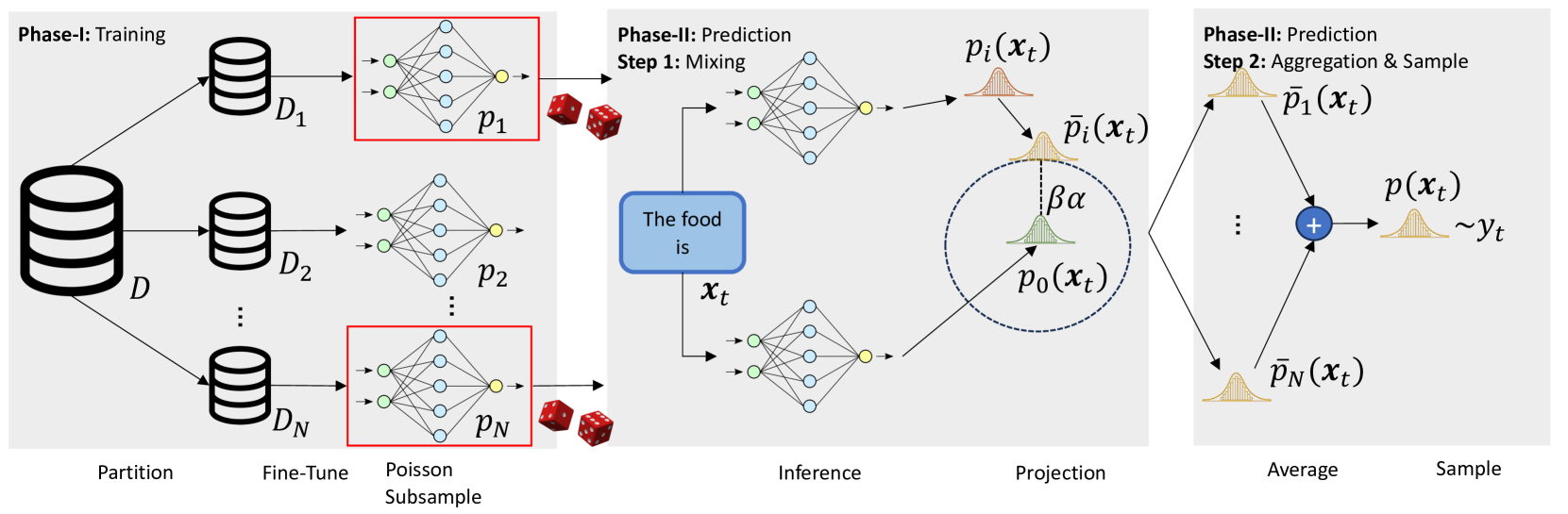
Figure 1: A brief overview of PMixED, which can be broken down into two phases. In Phase-I, the private dataset $D$ is partitioned into $N$ pairwise disjoint subsets $D_{1},...,D_{N}$, each of which $D_{i}$ is fine-tuned with a pre-trained LLM to produce $p_{i}$. Afterward, PMixED performs private predictions in Phase-II which can be further broken down into two steps. In Step 1, which we call mixing, a query $\mathbf{x}_{t}$ from a user is received at time $1\leq t\leq T$. First, PMixED subsamples a subset of the ensemble, then generates the output distribution of each selected model $p_{i}(\mathbf{x}_{t})$ and the output distribution of a public model $p_{0}(\mathbf{x}_{t})$. Each $p_{i}(\mathbf{x}_{t})$ is projected along a Renyi Divergence ball centered at the output distribution $p_{0}(\mathbf{x}_{t})$ with radius $\beta\alpha$ to produce $\overline{p}_{i}(\mathbf{x}_{t})$, which is a mixture of private $p_{i}(\mathbf{x}_{t})$ and public $p_{0}(\mathbf{x}_{t})$ information. In Step 2, all projected distributions are averaged into $p(\mathbf{x}_{t})$ then sampled $y_{t}\sim p(\mathbf{x}_{t})$.

A key observation that motivates this work is that many commercial deployments of LLMs are only accessible via an API, e.g. Chat-GPT. Hence, an adversary has only black-box access to the model, yet DP-SGD assumes the adversary has white-box access to the model since it applies differential privacy to the model parameters. Such a pessimistic assumption on adversarial capabilities can lead to overestimating the privacy loss bounds Nasr et al. (2021). We believe that improving the privacy of LLMs under the black box assumption is the key to enabling wider adoption of privacy-preserving LLMs. However, prior work has demonstrated that private prediction algorithms generally perform worse than private training algorithms van der Maaten and Hannun (2020).

To address the aforementioned limitations, we propose PMixED, depicted in Figure 1. Rather than providing DP during training, PMixED instead provides DP for a private corpus during inference by utilizing two crucial features: (1) Randomness comes for free when predicting the next-token by sampling from the output probability distribution of a language model; (2) We can bound the privacy leakage of a prediction using a public model to mix the predictions of privacy-sensitive LLMs. We formalize these two observations by introducing $(\alpha,\beta)$-RD Mollifiers which generalize $\epsilon$-Mollifers introduced in Husain et al. (2020) and could be of interest independent of this work.

PMixED can be broken down into two phases: training and private prediction. During Phase-I: training, PMixED follows the sample-and-aggregate paradigm Nissim et al. (2007) by partitioning a private corpus into $N$ pairwise disjoint subsets, then fine-tuning a pre-trained LLM on each subset to produce an ensemble. Using an ensemble is crucial for guaranteeing privacy, but also has been shown to boost perplexity Jozefowicz et al. (2016). During Phase-II: private prediction, PMixED selects a subset of the ensemble using Poisson subsampling. Each selected model produces its output probability distribution, then follows the RD-mollification process by projecting its output distribution onto a Renyi Divergence ball centered at a public model’s output distribution. Lastly, PMixED averages these optimal projections and then samples from it.

Because PMixED does not employ differentially private training algorithms, it does not incur substantial training overhead like DP-SGD. Furthermore, we reduce computational and storage costs by employing parameter-efficient fine-tuning methods. In summary, our key contributions are the following: (1) We introduce and formalize $(\alpha,\beta)$-RD Mollifiers, a generalization of $\epsilon$-Mollifers, to avoid additive DP noise. (2) We propose a private prediction protocol utilizing RD Mollifiers and prove that it satisfies the DP prediction definition with group-level privacy. (3) We experimentally demonstrate that PMixED outperforms DP-SGD on two large-scale datasets. (4) We open-source our software implementation of PMixED to further spark research in this area.

2 Related Works

Most of the previous differential privacy work in LLMs has focused on private training. McMahan et al. (2017) first explored private training of language models using a small recurrent neural network to achieve user-level differential privacy in the federated learning setting. Recent breakthroughs in differentially private LLMs involve self-supervised pre-training on public data, followed by privately fine-tuning on a private corpus Li et al. (2021); Yu et al. (2021).

An orthogonal approach, but conceptually similar to ours, is PATE Papernot et al. (2016, 2018). PATE also uses an ensemble of models trained on pairwise disjoint subsets of a private dataset to generate DP labels. However, PATE and PMixED rely on substantially different private aggregation schemes. PATE uses the Gaussian/Laplacian mechanism to perturb its output vote count histogram while our method utilizes the inherent stochastic nature of sampling from a probability distribution and a public model in LLMs. Furthermore, PATE does not satisfy the DP prediction definition Dwork and Feldman (2018) since its data-dependent privacy accounting causes its privacy loss to be a function of the private data. Hence, testing that the data-dependent loss does not exceed the privacy budget will leak additional privacy Redberg et al. (2023).

There is a much smaller body of work that has focused on private prediction for generative language models, mainly due to prior work empirically showing that private prediction methods perform worse than private training van der Maaten and Hannun (2020). Private prediction can be broadly categorized into two methods: prediction sensitivity, which adds noise to the output distribution of an LLM; and sample-and-aggregate, which involves the same process as PATE for generating noisy labels. For prediction sensitivity, Majmudar et al. (2022) used the uniform distribution as their perturbation mechanism and showed that it satisfies $\epsilon$-DP. However, the privacy loss needs to be large, $\epsilon\approx 60$, in order to be practical.

One work closely related to PMixED, which motivated our work, also falls under the sample-and-aggregate method as ours Ginart et al. (2022). However, their ensemble could exceed the privacy budget before completing all $T$ queries due to their data-dependent privacy accounting. Hence, they had to define a new privacy notion to account for this. Our work does not have this limitation.

3 Preliminaries

3.1 Next-Token Prediction Task

Given some context vector $\mathbf{x}_{t}=x_{1},x_{2},...,x_{t}$, which is a string of tokens from some vocabulary $V$, i.e. $x_{i}\in V$ for all $i=1,...,t$, the task is to predict the next token $x_{t+1}$ using a generative language model $p$. More precisely, the output of a language model $p$ for a given context $\mathbf{x}_{t}$ is a likelihood function of all possible tokens $p(x_{t+1}=w|\mathbf{x}_{t})$, and choosing the next token involves sampling from this probability mass function to obtain a token $\hat{x}_{t+1}\sim p(x_{t+1}|\mathbf{x}_{t})$.

3.2 Differential Privacy

If a machine learning model has memorized any sensitive information that is contained in its training data, then it can potentially reveal this information during prediction. Differential Privacy (DP) is a mathematical framework that gives privacy guarantees for this type of privacy leakage by reducing the effect any individual has on a model.

Definition 3.1 (Approximate DP Dwork et al. (2014)).

More formally, let $\epsilon>0,\delta\in[0,1]$. A randomized algorithm $A:\mathcal{D}\rightarrow\mathcal{R}$ satisfies $(\epsilon,\delta)$-DP if for any pair of adjacent datasets $D,D^{{}^{\prime}}\in\mathcal{D}$ and any set of subset of outputs $S\subseteq\mathcal{R}$ it holds that:

$$\Pr[A(D)\in S]\leq e^{\epsilon}\Pr[A(D^{{}^{\prime}})\in S]+\delta.$$

The privacy parameters $\epsilon,\delta$ can be interpreted as follows: $\epsilon$ upper bounds the privacy loss, and $\delta$ is the probability that this guarantee does not hold. One subtle, but crucial, technicality is that adjacency can be achieved at any granularity. E.g., $D^{\prime}$ adds or removes $k$ entries from $D$, which is known as the "add\remove" scheme, or $D$ and $D^{\prime}$ differ by $k$ entries where $0<k\leq n$, which is known as the replacement scheme. Technically, both schemes are equivalent but for this work, we focus on the "add\remove" scheme.

Renyi DP (RDP), another notion of DP, contains composition properties that are easier to work with than $(\epsilon,\delta)$-DP Mironov (2017). To define RDP, we first define Renyi Divergence.

Definition 3.2 (Renyi Divergence Mironov (2017)).

For two probability distributions $P$ and $Q$ defined over $\mathcal{R}$, the Renyi divergence of order $\alpha>1$ is

$$D_{\alpha}(P||Q)=\frac{1}{\alpha-1}\log\mathop{\mathbb{E}}_{x\sim Q}\left[\left(\frac{P(x)}{Q(x)}\right)^{\alpha}\right],$$ (1)

and $D_{\alpha}^{\leftrightarrow}(P||Q)=\max\{D_{\alpha}(P||Q),D_{\alpha}(Q||P)\}$.

Definition 3.3 ($(\alpha,\epsilon)$-RDPMironov (2017)).

A randomized algorithm $A:\mathcal{D}\rightarrow\mathcal{R}$ is $(\alpha,\epsilon)$-RDP if for any adjacent datasets $D,D^{{}^{\prime}}\in\mathcal{D}$ it holds that

$$D_{\alpha}(A(D)||A(D^{{}^{\prime}}))\leq\epsilon.$$ (2)

RDP possesses useful properties which we will make use of in our privacy analysis and discuss in Appendix C.

3.3 Private Training vs. Private Prediction

We say that $A$ is a private training algorithm if it produces weights that are differentially private with respect to a private corpus $D$. For DP-SGD, $A(D)$ returns the per-sample gradients of the parameters perturbed with Gaussian noise for each iteration of training. Private training algorithms provide strong privacy since they limit privacy leakage even when an adversary has complete, white-box access to the model parameters.

We observe that commercial deployments of LLMs are typically cloud-based and the model is only accessible through API, so an adversary does not have access to model parameters. In this black box setting an alternative approach, called private prediction Dwork and Feldman (2018), provides DP at prediction, which exploits this important relaxation. We formalize this below:

Definition 3.4 (Privacy-Preserving Prediction).

Let $A$ be a non-private training algorithm such that $p=A(D)$, $Q$ be an interactive query generating algorithm that generates queries $\mathbf{x}_{t}$, and $\mathcal{P}$ be a protocol that responds with $y_{t}\in V$. Define the output $(Q\rightleftharpoons_{T}\mathcal{P}(\theta))=\{(\mathbf{x}_{t},y_{t})\}_{t=1}^{T}$ as a sequence query-response pairs where $T>0$ is some positive integer. Then $\mathcal{P}$ is a private prediction protocol if $(Q\rightleftharpoons_{T}\mathcal{P}(\theta))$ is $(\alpha,\epsilon)$-RDP, i.e., for adjacent datasets $D,D^{{}^{\prime}}$ with $p=A(D)$ and $p^{\prime}=A(D^{{}^{\prime}})$:

$$D_{\alpha}((Q\rightleftharpoons_{T}\mathcal{P}(p)||(Q\rightleftharpoons_{T}\mathcal{P}(p^{\prime})))\leq\epsilon.$$

Note that due to the Post-Processing Theorem C.1, any predictions made by a privately-trained model are differentially private. Alternatively, the goal of our work, given a private budget $\epsilon_{G}$, is to develop a protocol $\mathcal{P}$ that uses a non-private model $p$ to make $(\alpha,\epsilon_{G})$-RDP predictions on a sequence of queries $\{\mathbf{x}_{t}\}_{t=1}^{T}$.

4 PMixED: A Protocol For Private Next Token Prediction

We now introduce and describe PMixED, a private prediction protocol for next token prediction. First, we will introduce a concept called Renyi Divergence (RD) Mollifiers, which formalize the projection of a private distribution onto a set around a public distribution, and help us prove the privacy guarantees of PMixED. Next, we will discuss the fine-tuning process of the ensemble, which follows the sample-and-aggregate paradigm. Lastly, we will describe the prediction protocol and show its privacy guarantees.

4.1 Renyi Divergence Mollifiers

Results from Ginart et al. (2022); Majmudar et al. (2022) showed that perturbing the output probability distribution of an LLM with noise significantly degrades the performance. We take a different approach by leveraging the inherent probabilistic nature of next-token prediction, which involves sampling the output distribution of an LLM. Hence, the output distribution of each fine-tuned LLM is mixed with the output distribution of a public LLM, thereby reducing the memorization obtained by fine-tuning. More formally, a privacy-sensitive distribution $P$ is projected onto a given RD mollifier, which is a set of distributions such that the Renyi Divergence of any pair of distributions in this mollifier does not diverge by too much while preserving the modes of $P$. This is pictorially shown in figure 2, and we formally define this below:

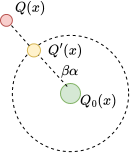
Figure 2: Left: Projecting a distribution $P$ (blue curve) onto an $(\alpha,\beta)$-RD mollifier (black curve). The dotted line represents the maximum divergence $\beta\alpha$ of the mollifier. Note how the projected distribution maintains the same modes as $P$. Right: $Q^{\prime}$ is the maximized projection of $Q$ onto a relative RD-mollifier around $Q_{0}$, which diverges by at most $\beta\alpha$ from $Q_{0}$.

Definition 4.1 ($(\alpha,\beta)$-RD Mollifier).

Let $\mathcal{M}\subset\mathcal{D}(\mathcal{X})$ be a set of distributions and $\alpha>1,\beta>0$. Then $\mathcal{M}$ is an $(\alpha,\beta)$-RD mollifier iff for all $Q,Q^{{}^{\prime}}\in\mathcal{M}$, $x\in\mathcal{X}$

$$D_{\alpha}(Q(x)||Q^{{}^{\prime}}(x))\leq\beta\alpha.$$ (3)

For example, the singleton $\mathcal{M}=\{Q\}$ is an $(\alpha,0)$-RD mollifier. Note that an $\epsilon$-Mollifier from Husain et al. (2020) is also an $(\alpha,\frac{1}{2}\epsilon^{2})$-RD mollifer for all $\alpha$ by the conversion from pure to zero concentrated DP Bun and Steinke (2016). RD-mollifiers consist of distributions that are close to each other with respect to the Renyi Divergence. Husain et al. (2020) states that deriving mollifiers is not always clear, but one way is to start from a reference distribution $Q_{0}$ and consider the set of all distributions that are close to $Q_{0}$, which we define below:

Definition 4.2 ($(\alpha,\beta)$-RD Mollifier relative to $Q_{0}$).

Let $\mathcal{M}_{(\alpha,\beta),Q_{0}}\subset\mathcal{D}(\mathcal{X})$ be a set of distributions. Then for all $Q\in\mathcal{M}_{(\alpha,\beta),Q_{0}}$

$$D_{\alpha}^{\leftrightarrow}(Q(x)||Q_{0}(x))\leq\beta\alpha.$$

Lemma 4.1.

If $\mathcal{M}_{(\alpha,\beta),Q_{0}}$ is an $(\alpha,\beta)$-RD Mollifier relative to $Q_{0}$, then $\mathcal{M}_{(\alpha,\beta),Q_{0}}$ is an $(\alpha,4\beta)$-RD Mollifer.

Proof. A straightforward application of the Triangle-like inequality property of Renyi Divergence, Theorem C.5. ∎

The goal then becomes taking a distribution $P$ and finding a distribution $\hat{P}$ inside a given mollifier $\mathcal{M}$ that minimizes the RD divergence:

$$\hat{P}\in\operatorname*{arg\,min}_{Q\in\mathcal{M}}D_{\alpha}(P||Q).$$ (4)

This process is called RD-mollification. In the following subsection, we will describe a mollification mechanism that takes a privacy-sensitive distribution $P$ as input and outputs a mollified distribution $\hat{P}$ that maximizes utility by finding the closest distribution to $P$ in a given mollifier.

4.2 Fine-tuning a Pre-trained Model

Suppose we have access to a non-private training procedure $A$, which takes as input a private dataset $D$ and a set of pre-trained weights $p_{0}$. Then $A(D,p_{0})$ returns a set of weights that have been fine-tuned on $p_{0}$ using $D$. Our instantiation of the fine-tuning process utilizes LoRA for parameter efficiency Hu et al. (2021), however, any fine-tuning method can be used. First we partition a private dataset $D$ into $N$ subsets $D_{1},D_{2},...D_{N}$ such that they are pairwise disjoint, i.e., $D_{i}\cap D_{j}=\varnothing$ for $i\neq j$, and $|D_{i}|=|D|/N$. Then for each subset $D_{i}$, we fine-tune $p_{0}$ using our training procedure $A$ to produce $p_{i}=A(D_{i},p_{0})$.

We want to highlight why LoRA is the natural parameter-efficient fine-tuning method to apply in this setting, and how it makes an ensemble of LLMs practical. Although PMixED conceptually produces $N$ models by the end of the fine-tuning process, using LoRA in our implementation only needs one model for inference, which is the pre-trained model $p_{0}$ combined with a set of LoRA adapter weights $p_{i}$. So when the $i$-th model performs inference, we just replace the LoRA weights with $p_{i}$ while still using the pre-trained model $p_{0}$.

4.3 Differentially Private Prediction Protocol

Given a sequence of queries $\{\mathbf{x}_{t}\}_{t=1}^{T}$, PMixED responds to each query $\mathbf{x}_{t}$ in a differentially private manner. This is succinctly summarized in Algorithm 1 and is broken down into three steps:

Algorithm 1 PMixED: A protocol for Private Next Token Prediction

Input. Number of LLMs $N$, Fine-Tuned LLM’s $\{p_{i}\}_{i=1}^{N}$, public model $p_{0}$, total number of queries $T$, privacy budget $\epsilon_{G}>0$, Renyi Divergence order $\alpha>1$, subsample probability $0<q\leq 1$, a series of queries $\{\mathbf{x}_{t}\}_{t=1}^{T}$, Subsampled privacy loss function $\epsilon^{\prime}_{q}(\alpha)$

1:for $t=1,...,T$ do

2:     Select a subset $S_{t}\subseteq[N]$ by choosing each model with probability $q$.

3:     $\beta\leftarrow\operatorname*{arg\,max}_{\beta^{\prime}}\left\{\epsilon^{\prime}_{q}(\alpha)\leq\epsilon_{G}/T\right\}$

4:     for $i\in S_{t}$ do

5:         $\lambda_{i}\leftarrow$ using eq. 5

6:         $\overline{p}_{i}(\mathbf{x}_{t})=\lambda_{i}p_{i}(\mathbf{x}_{t})+(1-\lambda_{i})p_{0}(\mathbf{x}_{t})$

7:     end for

8:     $p(\mathbf{x}_{t})=p_{0}(\mathbf{x}_{t})$

9:     if $S_{t}\neq\emptyset$ then

10:         $p(\mathbf{x}_{t})=\frac{1}{|S_{t}|}\sum\limits_{i\in S_{t}}\overline{p}_{i}(\mathbf{x}_{t})$

11:     end if

12:     $y_{t}\sim p(\mathbf{x}_{t})$

13:end for

14:return $\{y_{1},...,y_{T}\}$

Poisson Subsampling of Ensemble.

We perform Poisson subsampling on the entire ensemble $\{p_{i}\}_{i=1}^{N}$ to obtain a subset of the ensemble $S_{t}\subseteq[N]$ such that each model $p_{i}$ is selected with probability $q$. The benefit of subsampling a subset of the ensemble is that it can further amplify the privacy of our protocol, since running on some random subset of the ensemble introduces additional uncertainty. In particular, if a protocol is $(\epsilon,\delta)$-DP then with subsampling probability $q$ it is roughly $(O(q\epsilon),q\delta)$-DP Steinke (2022). In the case that no models are sampled, PMixED resorts to the public model $p_{0}$ for prediction entirely.

Inference and RD-Mollification.

Each sampled model $i\in S_{t}$ performs inference to produce an output distribution $p_{i}(\mathbf{x}_{t})$. Then we RD-mollify each distribution $p_{i}(\mathbf{x}_{t})$ by mixing it with the public distribution $p_{0}(\mathbf{x}_{t})$ using a mixing parameter $\lambda_{i}$ to produce $\overline{p}_{i}(\mathbf{x}_{t})=\lambda_{i}p_{i}(\mathbf{x}_{t})+(1-\lambda_{i})p_{0}(\mathbf{x}_{t})$. $\lambda_{i}$ is automatically chosen by solving the following optimization scheme:

$$\lambda_{i}\leftarrow\operatorname*{arg\,max}\limits_{\lambda\in[0,1]}\{D_{\alpha}^{\leftrightarrow}(\overline{p}_{i}(\mathbf{x}_{t})||p_{0}(\mathbf{x}_{t}))\leq\beta\alpha\}.$$ (5)

The value of $\beta$ will be specified once we state the privacy guarantees of our protocol. We opt to numerically solve Equation 5 by using the bisection method from the SciPy library. Note that as we increase $\lambda_{i}$, the function $D_{\alpha}^{\leftrightarrow}(\overline{p}_{i}(\mathbf{x}_{t})||p_{0}(\mathbf{x}_{t}))$ will increase because $\overline{p}_{i}(\mathbf{x}_{t})$ diverges more from $p_{0}(\mathbf{x}_{t})$ and approaches $p_{i}(\mathbf{x}_{t})$. Hence $D_{\alpha}^{\leftrightarrow}(\overline{p}_{i}(\mathbf{x}_{t})||p_{0}(\mathbf{x}_{t}))$ is monotonically increasing with respect to $\lambda_{i}$, which allows us to use bisection for this function. Moreover, each of the projected distributions is an element in the RD-Mollifer relative to $p_{0}(\mathbf{x}_{t})$, i.e., $\overline{p}_{i}(\mathbf{x}_{t})\in\mathcal{M}_{(\alpha,\beta),p_{0}(\mathbf{x}_{t})}$ for all $i\in[N]$, which satisfies Equation 4, giving us the optimal projection.

Aggregation and Sampling.

The last step is to average the projected distributions, then sample from this averaged distribution:
$y_{t}\sim\frac{1}{|S_{t}|}\sum\limits_{i\in S_{t}}\lambda_{i}p_{i}(\mathbf{x}_{t})+(1-\lambda_{i})p_{0}(\mathbf{x}_{t})$.

5 Privacy Analysis

We begin our privacy analysis of PMixED by first considering the case of no Poisson subsampling. Then we invoke the privacy amplification theorem C.4 to derive our final privacy guarantees. Lastly, we will discuss the implications of our privacy guarantees. Let $\mathcal{P}$ denote our private prediction protocol, PMixED. Note that $D$ and $D^{{}^{\prime}}$ are neighboring datasets if $D^{{}^{\prime}}$ adds or removes a subset $D_{i}$ from $D$, which is equivalent to adding or removing the model $p_{i}$ from the ensemble.

5.1 DP Guarantees for PMixED

At a high level, we will prove that $\mathcal{P}$ is $(\alpha,\epsilon_{G}/T)$-RDP for query $\mathbf{x}_{t}$. Then, using the Composition Theorem C.2, we can say that $\mathcal{P}$ is $(\alpha,\epsilon_{G})$-RDP for query-responses $\{(\mathbf{x}_{t},y_{t})\}_{t=1}^{T}$, thus satisfying the Private Prediction Definition 3.4. Appendix B analyzes the case when $\alpha=\infty$, which is pure DP. Essentially, $D_{\alpha}(p(\mathbf{x}_{t})||p_{-i}(\mathbf{x}_{t}))$ gives an upper bound while $D_{\alpha}(p_{-i}(\mathbf{x}_{t})||p(\mathbf{x}_{t}))$ gives a lower bound for $\beta$ . Thus, it suffices to show $D_{\alpha}(p(\mathbf{x}_{t})||p_{-i}(\mathbf{x}_{t}))\leq\epsilon_{G}/T$.

Theorem 5.1.

Let

$$\beta\leq\begin{cases}\frac{\log\left(Ne^{(\alpha-1)\epsilon_{G}/T}+1-N\right)}{4(\alpha-1)\alpha},&\text{if }N>1\\ \frac{\epsilon_{G}}{T\alpha}&\text{otherwise}\end{cases}.$$ (6)

Then the output of PMixED $\mathcal{P}$ on query $\mathbf{x}_{t}$ is $(\alpha,\epsilon_{G}/T)$-RDP with respect to $D$.

Proof. Let $i\in[N]$ and $\mathbf{x}_{t}$ be a query. Define

$$p(\mathbf{x}_{t})=\frac{1}{N}\sum_{i=1}^{N}\lambda_{i}p_{i}(\mathbf{x}_{t})+(1-\lambda_{i})p_{0}(\mathbf{x}_{t}),$$

$$p_{-i}(\mathbf{x}_{t})=\frac{1}{N-1}\sum_{j\neq i}\lambda_{j}p_{j}(\mathbf{x}_{t})+(1-\lambda_{j})p_{0}(\mathbf{x}_{t})$$

where $\lambda_{i}$ is selected from Equation 5. Now, observe that each $\lambda_{i}$ is dependent only on $D_{i}$, so $p_{-i}(\mathbf{x}_{t})$ does not contain $D_{i}$. Using the fact that $D_{\alpha}^{\leftrightarrow}(p_{j}(\mathbf{x}_{t})||p_{0}(\mathbf{x}_{t}))\leq\beta\alpha$ for all $j\in[N]$, then for any two neighboring ensembles $\{p_{i}\}_{i=1}^{N}$, $\{p_{j}\}_{j\neq i}$ with $N>1$

$$e^{(\alpha-1)D_{\alpha}\left(y_{t}\sim\mathcal{P}\left(\{p_{i}\}_{i=1}^{N},\mathbf{x}_{t}\right)||y_{t}\sim\mathcal{P}\left(\{p_{j}\}_{j\neq i},\mathbf{x}_{t}\right)\right)}$$

$$=e^{(\alpha-1)D_{\alpha}(p(\mathbf{x}_{t})||p_{-i}(\mathbf{x}_{t}))}$$

$$=\mathop{\mathbb{E}}_{p_{-i}(\mathbf{x}_{t})}\left[\left(\frac{p(\mathbf{x}_{t})}{p_{-i}(\mathbf{x}_{t})}\right)^{\alpha}\right]$$

$$=\mathop{\mathbb{E}}_{p_{-i}(\mathbf{x}_{t})}\left[\left(\frac{\frac{N-1}{N}p_{-i}(\mathbf{x}_{t})+\frac{1}{N}\overline{p}_{i}(\mathbf{x}_{t})}{p_{-i}(\mathbf{x}_{t})}\right)^{\alpha}\right]$$

$$\leq\mathop{\mathbb{E}}_{p_{-i}(\mathbf{x}_{t})}\left[\frac{\frac{N-1}{N}(p_{-i}(\mathbf{x}_{t}))^{\alpha}+\frac{1}{N}(\overline{p}_{i}(\mathbf{x}_{t}))^{\alpha}}{(p_{-i}(\mathbf{x}_{t}))^{\alpha}}\right]$$ (7)

$$=\mathop{\mathbb{E}}_{p_{-i}(\mathbf{x}_{t})}\left[\frac{N-1}{N}+\frac{1}{N}\left(\frac{\overline{p}_{i}(\mathbf{x}_{t})}{p_{-i}(\mathbf{x}_{t})}\right)^{\alpha}\right]$$

$$=\frac{N-1}{N}+\frac{1}{N}\mathop{\mathbb{E}}_{p_{-i}(\mathbf{x}_{t})}\left[\left(\frac{\overline{p}_{i}(\mathbf{x}_{t})}{p_{-i}(\mathbf{x}_{t})}\right)^{\alpha}\right]$$

$$=\frac{N-1}{N}+\frac{1}{N}e^{(\alpha-1)D_{\alpha}(\overline{p}_{i}(\mathbf{x}_{t})||p_{-i}(\mathbf{x}_{t}))}$$

$$\leq\frac{N-1}{N}+\frac{1}{N}e^{(\alpha-1)4\beta\alpha}$$ (8)

where Equation 7 uses Jensen’s inequality for the convex function $f(x)=x^{\alpha}$ since $\alpha\geq 1$ and $x\geq 0$ because we are dealing with probabilities, and Equation 8 is due to $D_{\alpha}(\overline{p}_{i}(\mathbf{x}_{t})||p_{0}(\mathbf{x}_{t}))\leq\beta\alpha$ and

$$D_{\alpha}(p_{0}(\mathbf{x}_{t})||p_{-i}(\mathbf{x}_{t})) \leq\max_{j\neq i}D_{\alpha}(p_{0}(\mathbf{x}_{t})||\overline{p}_{j}(\mathbf{x}_{t}))$$

$$\leq\beta\alpha$$

by the Quasi Convexity property of Renyi Divergence C.6. Then using the Triangle-like Inquality C.5 gives us $D_{\alpha}(\overline{p}_{i}(\mathbf{x}_{t})||p_{-i}(\mathbf{x}_{t}))\leq 4\beta\alpha$. Hence plugging in Equation 6 for $\beta$ into Equation 8 implies $D_{\alpha}(p(\mathbf{x}_{t})||p_{-i}(\mathbf{x}_{t}))\leq\epsilon_{G}/T$. When $N=1$, then $p_{-i}(\mathbf{x}_{t})=p_{0}(\mathbf{x}_{t})$ since our protocol will resort to using $p_{0}$. Hence $D_{\alpha}(p(\mathbf{x}_{t})||p_{-i}(\mathbf{x}_{t}))\leq\beta\alpha\leq\epsilon_{G}/T$. Thus proves the claim that the output of $\mathcal{P}$ on query $\mathbf{x}_{t}$ is $(\alpha,\epsilon_{G}/T)$-RDP. ∎

Theorem 5.2.

PMixED $\mathcal{P}$ is an $(\alpha,\epsilon_{G})$-RDP prediction protocol with respect to $D$.

Proof. Let $Q$ be an interactive query generating algorithm that generates queries $\mathbf{x}_{t}$. We first obtain fine-tuned weights using our training algorithm $p_{i}=A(p_{0},D_{i})$. Then $\mathcal{P}$ uses $\mathbf{x}_{t}$ as input and returns a response, which is a sample $y_{t}\sim\mathcal{P}(\{p_{i}\}_{i=1}^{N},\mathbf{x}_{t})$. By Theorem 5.1, $y_{t}$ is $(\alpha,\epsilon_{G}/T)$-RDP. Then after $T$ queries and responses, the sequence $\{(\mathbf{x}_{t},y_{t})\}_{t=1}^{T}$ is $(\alpha,\epsilon_{G})$-RDP by the Composition Theorem C.1. Therefore $\mathcal{P}$ is an $(\alpha,\epsilon_{G})$-RDP prediction protocol. ∎

A few observations to highlight: (1) $\beta$ depends on the number of models in the ensemble $N$. As $N$ increases, then $\beta$ also becomes larger. Intuitively, each model has less effect on the overall output, which allows them to diverge more from the public model. Also note that the choice of $N$ is fixed by the analyst, independent of the dataset. Hence $\beta$ does not leak information about the dataset.

(2) Our analysis also relies on the fact that PMixED employs ancestral sampling as its decoding strategy, which samples directly from the ensemble’s per query distribution, $p(\mathbf{x}_{t})$. Truncated decoding such as top-k Fan et al. (2018) or top-p Holtzman et al. (2019) sampling which samples only plausible tokens in the distribution, and greedy decoding which only samples the most likely next token, could be employed to improve the text generation quality. However, additional privacy leakage can occur, so we leave it as a future work to extend PMixED to these decoding strategies.

5.2 DP Guarantees for Subsampled PMixED

Now that we have shown that $\mathcal{P}$ is an $(\alpha,\epsilon_{G})$-RDP prediction protocol with the "add\remove" scheme, PMixED is compatible with the Privacy Amplification by Poisson Subsampling Theorem C.4. Let $S_{t}$ be the subsampled set at time $t$ where $p_{S_{t}}$ is $(p_{S_{t}})_{i}=p_{i}$ if $i\in S_{t}$ and $(p_{S_{t}})_{i}=\bot$ if $i\notin S_{t}$. Let $\mathcal{P}^{S_{t}}$ be the subsampled PMixED protocol where $\mathcal{P}^{S_{t}}(p,\mathbf{x}_{t})=\mathcal{P}(p_{S_{t}},\mathbf{x}_{t})$. Then by Theorem C.4, the output of $\mathcal{P}^{S_{t}}$ on query $\mathbf{x}_{t}$ is $(\alpha,\epsilon^{\prime}_{q}(\alpha))$-RDP where $\epsilon^{\prime}_{q}(\alpha)$ is defined in Equation 12.

Since $\epsilon^{{}^{\prime}}_{q}(\alpha)\ll\epsilon_{G}/T$, we can increase $\epsilon^{{}^{\prime}}_{q}(\alpha)$ to be as close to $\epsilon_{G}/T$ as possible by increasing $\epsilon(\alpha)$, the privacy loss of $\mathcal{P}$, using $\beta$. In other words, the privacy loss of PMixED is

$$\epsilon(\alpha)\leq\begin{cases}\frac{\log\left(\frac{|S_{t}|-1+\exp\left({(\alpha-1)4\beta\alpha}\right)}{|S_{t}|}\right)}{\alpha-1}&\text{if }|S_{t}|>1\\ \beta\alpha&\text{otherwise}\end{cases}.$$

Hence, PMixED uses $\epsilon(\alpha)$ to solve the following equation: $\beta^{*}=\operatorname*{arg\,max}_{\beta}\left\{\epsilon^{\prime}_{q}(\alpha)\leq\epsilon_{G}/T\right\}$, which selects the optimal RD radius $\beta^{*}$.

5.3 Privacy Level Granularity

Seemingly, PMixED is stronger than sample level privacy since $D_{\alpha}^{\leftrightarrow}(\mathcal{P}(D)||\mathcal{P}(D\setminus\{d\}))\leq D_{\alpha}^{\leftrightarrow}(\mathcal{P}(D)||\mathcal{P}(D\setminus D_{i}))$ for some sample $d\in D_{i}$ and $i\in[N]$, due to the group privacy property Mironov (2017). In actuality, our method is closely related to group-level privacy Ponomareva et al. (2023), where each subset $D_{i}$ defines a group of samples, and each sample is contained in exactly one group. This flexibility allows PMixED to offer different granularities of privacy, depending on the partitioning of the private corpus. For example, PMixED is compatible with virtual client-level privacy Xu et al. (2023), a stronger version of user-level privacy, where a subset $D_{i}$ is considered a virtual client comprised of groups of user data, and each user’s data is stored in at most one subset. For practical language modeling datasets where users can contain multiple data samples, guaranteeing sample-level privacy is insufficient to ensure the privacy of an individual user McMahan et al. (2017). Hence, for these types of datasets, PMixED can provide a strong enough privacy guarantee for users. We delegate dataset partitioning, consequently determining the privacy level, to the practitioner.

6 Experiments

Parameter	Value
Privacy Budget: $\epsilon_{G}$	8
Runs:	$32$
Probability of Failure: $\delta$	1e-5
Renyi Divergence Order: $\alpha$	3
Inference Budget: $T$	1024
Number of Ensembles: $N$	80
Subsample Probability: $p$	0.03

Table 1: Privacy Hyperparameters for PMixED and DP-SGD.

6.1 Experimental Setup

We experimentally evaluated the privacy-utility tradeoff of PMixED by using LoRA Hu et al. (2021) to fine-tune pre-trained GPT-2 models Radford et al. (2019) from HuggingFace Wolf et al. (2019) on the WikiText-103 Merity et al. (2016) and One Billion Word Chelba et al. (2013) datasets. We view these two large word-level English language modeling benchmarks as complementary to each other, in that they give a good comprehensive evaluation of differentially private next token prediction. WikiText-103 tests the ability of long-term dependency modeling, while One Billion Word mainly tests the ability to model only short-term dependency Dai et al. (2019).

The public model in our experiments is a pre-trained GPT-2 small model. We compare PMixED to three baselines: the public model, a non-private fine-tuned model, and a private fine-tuned model produced by DP-SGD. Although DP-SGD has a weaker privacy level, we compared PMixED to per-sample DP-SGD as our baseline because it illustrates how well PMixED performs against the most widely-used DP solution. The non-private and private fine-tuned baselines also used LoRA. LoRA based fine-tuning can outperform full private fine-tuning since the LoRA updates a much smaller set of parameters during fine-tuningYu et al. (2021). The LoRA parameters used for each model $p_{i}$ contain $0.11\%$ of the total number of parameters of the pre-trained model, allowing us to fit the entire ensemble into one GPU during prediction. Appendix A contains more details about fine-tuning.

For private prediction, unless stated otherwise, the parameters used are set to the default values shown in Table 1. The privacy hyperparameters are reported in terms of $(\epsilon_{G},\delta)$-DP, however we perform our privacy loss calculations in terms of RDP, then convert back using Theorem C.3. To measure the utility, we use test-set perplexity with a sequence length of $512$. In total, $T$ predictions are made for each run, and a total of $32$ runs are performed and averaged for each baseline.

6.2 Comparison Over Baselines

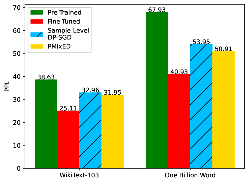
Figure 3: Comparison of PMixED against 3 baselines on WikiText-103 and One Billion Word using GPT-2.

The pre-trained and fine-tuned models represent two extremes in the privacy-utility spectrum: the pre-trained model is perfectly private but has no utility gain, while the fine-tuned model has the best utility but guarantees no privacy. Since PMixED is a mixture of both, its utility and privacy guarantees should be between both. Figure 3, which contains results of each baseline and PMixED on the test-set perplexity, shows that this is indeed the case. For the WikiText-103 dataset, the pre-trained model achieved a perplexity score of $38.63$, and the fine-tuned model achieved $25.11$. PMixED scored $31.95$ which is a $7$ point perplexity improvement over the pre-trained model, while guaranteeing $(\epsilon_{G},\delta)$-DP as opposed to the completely non-private fine-tuned model $\epsilon_{G}=\infty$. Furthermore, PMixED gains a $17$ point perplexity improvement over the pre-trained model for the One Billion Word dataset.

PMixED was also able to improve the perplexity score over DP-SGD by $1$ and $3$ points on the WikiText-103 and One Billion Word datasets, respectively. This result validates that private prediction methods can outperform private training for large query budgets van der Maaten and Hannun (2020). Moreover, the results of PMixED demonstrate that we can obtain the stronger group-level privacy without compromising utility.

6.3 Ablation Study

We explore the privacy hyperparameters used by PMixED for prediction on WikiText-103. $8$ runs are performed and averaged for each hyperparameter value, shown in Figure 4.

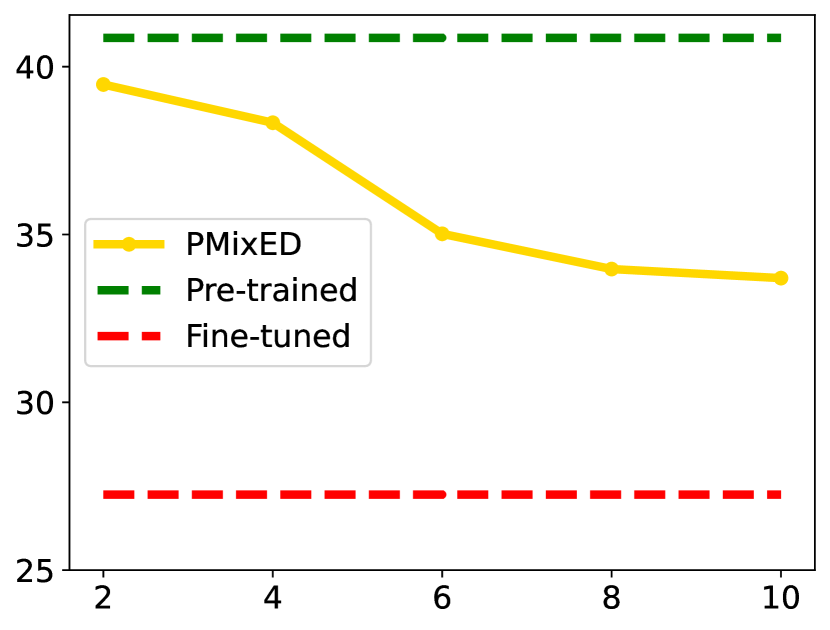
(a) epsilon

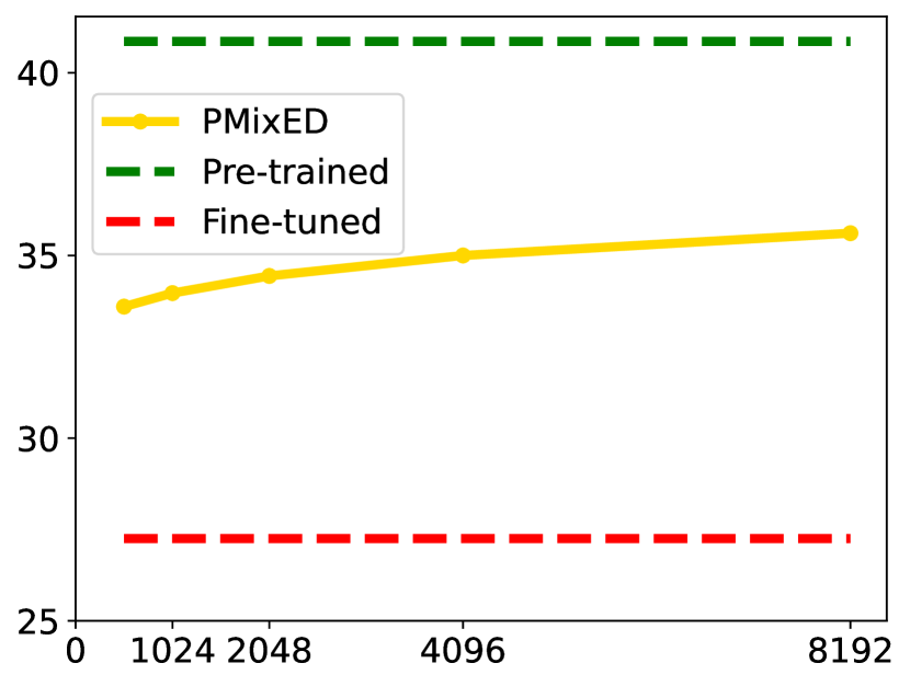
(b) query budget

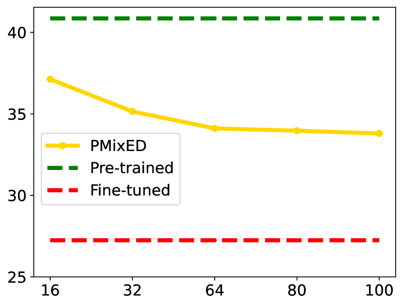
(c) ensemble

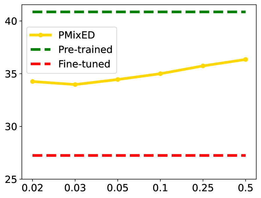
(d) probability

Figure 4: Ablation study on DP hyperparameters using WikiText-103. The x-axis is the hyperparameter space, and the y-axis is the perplexity score.

Figure 4(a) shows that for small privacy budgets $\epsilon_{G}\in[2,4]$, the utility of PMixED approaches the pre-trained model. This is due to the RD mollification producing projected distributions close to the public model because $\epsilon_{G}$ is too small, so $\alpha$ must be large causing $D_{\alpha}$ to decrease monotonically. For moderately sized privacy budgets $\epsilon_{G}\in[4,8]$, we see a sharp improvement in perplexity since $\alpha$ is smaller. Appendix D shows the relationship between $\alpha$ and perplexity. Figure 4(b) shows that even if the inference budget $T$ is as large as $T=8192$, we observe only marginal performance degradation of PMixED, losing only $1.6$ PPL from $T=1024$. Thus PMixED is capable of handling large amounts of inference while still being performant.

For the results in Figure 4(c), ensemble sizes $N=16,32,64$ were trained with $E=10$ epochs, while $N=80$ was trained with $E=15$ and $N=100$ with $E=20$. The trend seems to be that larger ensembles with increased training epochs lead to better performance. We surmise that larger ensembles increase the expected number of subsampled models. And more explicit memorization occurs with increasing epochs, which when mixed with the public model allows for better generalization, similar to Khandelwal et al. (2019). Eventually, too many models can lead to little training data to learn from, which we leave as future work to explore.

We conclude by remarking that in comparison to DP-SGD, the additional hyperparameters introduced by PMixED are the query budget $T$, the ensemble size $N$, and the subsample probability $q$. However, DP-SGD contains the clipping threshold and the expected subsample batch size as hyperparameters that PMixED does not need to work with. Therefore, since $T$ is determined based on the problem setup, PMixED does not add more hyperparameters than DP-SGD. Moreover, tuning the hyperparameters of PMixED is considerably faster compared to DP-SGD because $N$ and $q$ are tuned during prediction, as opposed to retraining an LLM for the tuning process of DP-SGD.

7 Conclusion and Future Directions

PMixED is inspired by the observation that most LLM deployments are cloud-based where an adversary only has black-box access to the model, rather than access to the entire model parameters. Under this setting, PMixED presents a novel private prediction protocol that provides DP during prediction, rather than during training. Thus PMixED is model agnostic, which has significant practical implications since it avoids the complexity of privately training models with millions or even billions of parameters. Our approach relies on an ensemble of fine-tuned LLMs and the novel idea of $(\alpha,\beta)$-RD Mollifiers, which generalizes $\epsilon$-Mollifers, to project each of the model’s output distribution onto a set around a public LLM’s output distribution.

PMixED is compatible with various privacy granularities, such as group-level DP, and is at least stronger than sample-level DP. Furthermore, PMixED does not require per-sample gradients and can operate on batch-level data, significantly reducing the training overhead compared to DP-SGD. We experimentally showed that PMixED outperforms DP-SGD in terms of utility on large-scale datasets using LLMs. Thus, PMixED substantially progresses private prediction methods in LLMs and offers a practical alternative to DP training methods.

Although our experiments only used a pre-trained GPT-2 small as the public model, in general, we can plug and play any public model for inference, highlighting the versatility of our approach. For example, we could use a GPT-2 model that is already fine-tuned on a public corpus from a different domain, or we could use a larger pre-trained model like GPT-2 XL. As a result, we can further boost the performance of our approach without additional training costs. We leave this exploration as a future work.

8 Limitations

PMixED performs better with larger ensemble sizes combined with longer training epochs, as quantified in the ablation studies. As ensemble sizes grow each model in the ensemble needs sufficient data to train, which in turn increases the cumulative training data size. We also note that PMixED requires more training epochs than regular SGD. However, these limitations are generally a bottleneck for all DP-based approaches, such as DP-SGD, and hence are not unique limitations of PMixED.

In this work, we employed LoRA to significantly reduce model size demands. However, storing an ensemble of models in memory can place a burden on the computing resources during training and inference procedures. The inference latency can be negatively impacted as an ensemble of models must provide predictions first followed by calculating the lambdas, due to the use of the bisection method. Potential systems optimizations can be to parallelize the inference and lambda calculations. We leave it as a future work to reduce the inference latency. But on the positive side, PMixED operates well with batch-based training and hence can take advantage of parallel GPU resources, while DP-SGD needs per-sample gradients which can curtail GPU efficiency.

Perhaps the biggest limitation of PMixED is the query budget, which limits the number of predictions that can be made. However, this limitation is a natural consequence of differentially private prediction from a nonprivately trained model. As a future work, one can explore a more relaxed problem setup, a PATE-like setting Papernot et al. (2016, 2018), where we produce DP predictions while minimizing the privacy loss.

Finally, we note how work in DP-SGD, as well as this work, uses a pre-trained model to boost performance. Unfortunately, using publicly available data is not necessarily risk-free in terms of privacy, as prior works were able to extract personally identifiable information from a GPT-2 model pre-trained on data scraped from the public internet Carlini et al. (2021). Thus model deployments must still be cautious of using pre-trained models in terms of understanding their information leakage potential.

9 Ethical Considerations

In this work, we utilized pre-trained large language models and well-known language modeling datasets that were accessed from the Hugging Face API, which are publicly available and free to use. The GPT-2 model and the One Billion Word Dataset are licensed under the Apache License, Version 2.0, and the WikiText-103 dataset is licensed under CC BY-SA 3.0. Our intended use of these artifacts is aligned with the intended use of the creators, which, for us, is purely for benchmarking our private next token prediction protocol, and does not trademark these artifacts. Since the datasets were originally obtained from public internet domains, and seemingly do not contain personally identifiable information, we did not anonymize the dataset. Our use of public models and datasets minimizes any unintended privacy leakage that could result from experimenting.

Additionally, we publicly released our code under the Apache License, Version 2.0. We believe that allowing open access to these experiments will help spark academic research of this work, as well as protect the privacy of user data in commercial deployment of large language models.

Appendix A Additional Experimental Details

The WikiText-103 dataset is a collection of over 100 million tokens from the set of verified Good and Bad articles on Wikipedia Merity et al. (2016). The One Billion Word dataset is text data obtained from the Sixth Workshop on Machine Translation, and it contains nearly one billion words in the training set Chelba et al. (2013). We split the datasets into sequences of length 512 tokens. A total of 920,344 examples are in the training set and 1928 in the validation set for WikiText-103. Table 2 displays the hyperparameter values used for fine-tuning. Certain hyperparameter values for non-private fine-tuning were selected from Hu et al. (2021), and certain hyperparameter values for private fine-tuning from Yu et al. (2021). We employed the AdamW optimizer with weight decay $0.01$ and a linear learning rate scheduler. Training ran on 8 Quadro RTX 5000, totaling around 8 hours for non-private fine-tuning, and 12 hours for private fine-tuning for WikiText-103. Prediction used only 1 Quadro RTX 5000.

There are technical challenges to get DP-SGD to contain the same privacy notion as ours. Either we would have to directly scale from sample-level privacy by the size of the partition $|D|/N$ using the group privacy property Dwork et al. (2014), which incurs a prohibitive privacy cost. Or directly clip and add noise to the per-subset gradients, which is not possible to implement with standard DP libraries, like Opacus.

Parameter	Fine-Tune	PMixED	DP-SGD
Epochs	3	151, 52	201, 92
Learning Rate	2e-4	2e-4	4e-4
Weight Decay	0.01	0.01	0.01
Adaptation $r$	4	4	4
LoRA $\alpha$	32	32	32
DP Batch Size	-	-	256
Clipping Norm	-	-	1.0

Table 2: Training Hyperparameters used for fine-tuning on ¹WikiText-103 and ²One Billion Word.

Appendix B Preliminary Setup for Theorem 5.1

Using our RD-mollifers concept, we introduce an additional concept called $(\alpha,\beta)$-RD private samplers, which is just $(\alpha,\beta)$-RDP but the neighboring condition is at the distributional level, then state how RD-mollifiers relates to RD-private samplers

Definition B.1 ($(\alpha,\beta)$-RD private sampler).

Let $\alpha>1,\epsilon>0$. An $(\alpha,\beta)$-RDP sampler is a randomized mapping $M:\mathcal{D}(\mathcal{X})\rightarrow\mathcal{X}$ such that for any $x\in\mathcal{X}$ and any two distributions $P,P^{{}^{\prime}}\in\mathcal{D}(\mathcal{X})$ we have

$$D_{\alpha}(M(P)||M(P^{\prime}))\leq\beta\alpha.$$ (9)

Lemma B.1.

Let $A:\mathcal{D}(\mathcal{X})\rightarrow\mathcal{X}$ be a randomized mechanism such that for any $P$, $A(P)$ releases a sample from some $Q\in\mathcal{M}$. If $\mathcal{M}$ is an $(\alpha,\beta)$-RD Mollifer, then $A$ is an $(\alpha,\beta)$-RDP sampler.

The proof of lemma B.1 is similar to the proof of the $\epsilon$-private sampler variant in Husain et al. (2020).

Since an $(\alpha,\beta)$-RD Mollifier implies an $(\alpha,\beta)$-RDP sampler, sampling from some distribution in a mollifier provides privacy. Hence, a naive privacy analysis can make use of the RD mollifier framework to derive the privacy loss, as is done in Husain et al. (2020). For each $\overline{p}_{i}(\mathbf{x}_{t}),\overline{p}_{i}^{\prime}(\mathbf{x}_{t})\in\mathcal{M}_{(\alpha,\beta),p_{0}}$, $D_{\alpha}(\overline{p}_{i}(\mathbf{x}_{t})||\overline{p}_{i}^{\prime}(\mathbf{x}_{t})\leq 4\beta\alpha$ due to lemma 4.1. Meaning, every projected distribution $\overline{p}_{i}(\mathbf{x}_{t})$ in the ensemble are $(\alpha,4\beta)$-RD samplers. Then sampling from the average of the projected distribution is still an $(\alpha,4\beta$)-RD sampler by the Post-Processing Theorem C.1. However, this privacy analysis is overly strict in that it’s a privacy guarantee where the neighboring ensembles can differ by all models except for one, which is too strong of a privacy notion. We are interested in the opposite neighborhood condition, where two ensembles are equal for all models except for one. This allows us to take advantage of the fact that the privacy cost of sampling from a mollifier is scaled by the inverse of the size of the ensemble.

Define $p_{-i}(\mathbf{x}_{t})=\frac{1}{N-1}\sum_{j\in[N]\setminus\{i\}}\lambda_{j}p_{j}(\mathbf{x}_{t})+(1-\lambda_{j})p_{0}(\mathbf{x}_{t})$. To show that sampling $y_{t}\sim p(\mathbf{x}_{t})$ is $(\alpha,\epsilon_{G}/T)$-RDP, i.e., $D_{\alpha}^{\leftrightarrow}(p(\mathbf{x}_{t})||p_{-i}(\mathbf{x}_{t}))\leq\frac{\epsilon_{G}}{T}$, first let’s look at a special case when $\alpha=\infty$ Now

$$e^{D_{\infty}(p(\mathbf{x}_{t})||p_{-i}(\mathbf{x}_{t}))}$$

$$=\frac{p(y_{t}|\mathbf{x}_{t})}{p_{-i}(y_{t}|\mathbf{x}_{t})}$$

$$=\frac{\frac{N-1}{N}p_{-i}(y_{t}|\mathbf{x}_{t})+\frac{1}{N}\overline{p}_{i}(y_{t}|\mathbf{x}_{t})}{p_{-i}(y_{t}|\mathbf{x}_{t})}$$

$$=\frac{N-1}{N}+\frac{1}{N}\frac{\overline{p}_{i}(y_{t}|\mathbf{x}_{t})}{p_{-i}(y_{t}|\mathbf{x}_{t})}$$

$$=\frac{N-1}{N}+\frac{1}{N}\frac{\overline{p}_{i}(y_{t}|\mathbf{x}_{t})}{p_{0}(y_{t}\mathbf{x}_{t})}\frac{p_{0}(y_{t}|\mathbf{x}_{t})}{p_{-i}(y_{t}|\mathbf{x}_{t})}$$

$$\leq\frac{N-1}{N}+\frac{1}{N}e^{2\beta\alpha}$$

for all $y_{t}\in V$. So if we want $D_{\infty}(p(\mathbf{x}_{t})||p_{-i}(\mathbf{x}_{t}))\leq\frac{\epsilon_{G}}{T}$ then we need set $\beta$ such that

$$\frac{N-1}{N}+\frac{1}{N}e^{2\beta\alpha} \leq e^{\frac{\epsilon_{G}}{T}}$$

$$e^{2\beta\alpha} \leq Ne^{\epsilon_{G}/T}+1-N$$

$$\beta \leq\frac{\log\left(Ne^{\epsilon_{G}/T}+1-N\right)}{2\alpha}.$$ (10)

For the other direction:

$$\frac{p_{-i}(y_{t}|\mathbf{x}_{t})}{p(y_{t}|\mathbf{x}_{t})} =\frac{\frac{N}{N-1}p(y_{t}|\mathbf{x}_{t})-\frac{1}{N-1}\overline{p}_{i}(y_{t}|\mathbf{x}_{t})}{p(y_{t}|\mathbf{x}_{t})}$$

$$=\frac{N}{N-1}-\frac{1}{N-1}\frac{\overline{p}_{i}(y_{t}|\mathbf{x}_{t})}{p(y_{t}|\mathbf{x}_{t})}$$

$$=\frac{N}{N-1}-\frac{1}{N-1}\frac{\overline{p}_{i}(y_{t}|\mathbf{x}_{t})}{p_{0}(y_{t}|\mathbf{x}_{t})}\frac{p_{0}(y_{t}|\mathbf{x}_{t})}{p(y_{t}|\mathbf{x}_{t})}$$

$$=\frac{N}{N-1}-\frac{1}{N-1}e^{2\beta\alpha}\leq e^{\epsilon_{G}/T}$$

$$e^{2\beta\alpha} \geq N-(N-1)e^{\epsilon_{G}/T}$$

$$\beta \geq\frac{\log(N-(N-1)e^{\epsilon_{G}/T})}{2\alpha}$$ (11)

for all $y_{t}\in V$. Equation 11 is satisfied by setting $\beta$ equal to eq. 10. Thus, it suffices to find $\beta$ with order $1<\alpha<\infty$ by working through $D_{\alpha}(p(\mathbf{x}_{t})||p_{-i}(\mathbf{x}_{t}))\leq\beta\alpha$, then set $\beta$ to its largest possible value so that $D_{\alpha}(p_{-i}(\mathbf{x}_{t})||p(\mathbf{x}_{t}))\leq\epsilon_{G}/T$.

Appendix C Properties of Renyi Divergence and RDP

Theorem C.1 (Post-Processing Mironov (2017)).

Let $A:\mathcal{D}\rightarrow\mathcal{R}$ be $(\alpha,\epsilon)$-RDP, and let $F:\mathcal{R}\rightarrow\mathcal{Z}$ be an arbitrary randomized mapping. Then $F\circ M$ is $(\alpha,\epsilon)$-RDP.

Theorem C.2 (Composition Mironov (2017)).

Let $A_{1},...,A_{k}$ be a sequence of $(\epsilon,\alpha)$-RDP algorithms. Then the composition $A_{k}\circ A_{k-1}\circ...\circ A_{1}$ is $(\alpha,k\epsilon)$-RDP.

Theorem C.3 (Conversion from RDP to Approximate DP Balle et al. (2020)).

If an algorithm $A$ is $(\alpha,\epsilon)$-RDP, then it is $(\epsilon+\log((\alpha-1)/\alpha)-(\log\delta+\log\alpha)/(\alpha-1),\delta)$-DP for any $0<\delta<1$.

Theorem C.4 (Tight Privacy Amplification by Poisson Subsampling for Renyi DP Steinke (2022)).

Let $U\subseteq[n]$ be a random set that contains each element independently with probability $q$. For $x\in\mathcal{X}^{n}$ let $x_{U}\in\mathcal{X}^{n}$ be given by $(x_{U})_{i}=x_{i}$ if $i\in U$ and $(x_{U})_{i}=\bot$ if $i\notin U$, where $\bot\in\mathcal{X}$ is some fixed value.

Let $\epsilon:\mathbb{N}_{\geq 2}\rightarrow\mathbb{R}\cup\{\infty\}$ be a function. Let $M:\mathcal{X}^{n}\rightarrow\mathcal{Y}$ satisfy $(\alpha,\epsilon(\alpha))$-RDP for all $\alpha\in\mathbb{N}_{\geq 2}$ with resepect to addition or removal– i.e., $x,x^{{}^{\prime}}\in\mathcal{X}^{n}$ are neighboring if, for some $i\in[n]$, we have $x_{i}=\bot$ or $x^{{}^{\prime}}_{i}=\bot$, and $\forall j\neq i$ $x_{j}=x_{j}^{{}^{\prime}}$.

Define $M^{U}:\mathcal{X}^{n}\rightarrow Y$ by $M^{U}(x)=M(x_{U})$. Then $M^{U}$ satisfies $(\alpha,\epsilon^{{}^{\prime}}_{q}(\alpha))$-RDP for all $\alpha\in\mathbb{N}_{\geq 2}$ where

$$\epsilon^{{}^{\prime}}_{q}(\alpha)=\frac{1}{\alpha-1}\log\left((1-q)^{\alpha-1}(1+(\alpha-1)q)\\ +\sum_{k=2}^{\alpha}\binom{\alpha}{k}(1-q)^{\alpha-k}q^{k}e^{(k-1)\epsilon(k)}\right).$$ (12)

Theorem C.5 (Triangle-like inequality, lemma 33.7 from Steinke (2022)).

Let $P,Q,R$ be distributions on $\mathcal{R}$. If $D_{\alpha}(P||Q)\leq\epsilon_{1}\alpha$ and $D_{\alpha}(Q||R)\leq\epsilon_{2}\alpha$ for $1<\alpha<\infty$, then

$$D_{\alpha}(P||R)\leq(\sqrt{\epsilon_{1}}+\sqrt{\epsilon_{2}})^{2}\alpha.$$ (13)

Theorem C.6 (Quasi-Convexity Steinke (2022)).

Let $P,Q,P{{}^{\prime}},Q^{{}^{\prime}}$ be probability distributions over $\mathcal{R}$ such that $P^{{}^{\prime}}$ absolutely continuous with respect to $Q^{{}^{\prime}}$. For $s\in[0,1]$, let $(1-s)P+sP^{{}^{\prime}}$ denote the convex combination of the distributions $P$ and $P^{{}^{\prime}}$ with weighting $s$. For all $\alpha\in(1,\infty)$ and all $s\in[0,1]$,

$$D_{\alpha}((1-s)P+sP^{{}^{\prime}}||(1-s)Q^{{}^{\prime}}+sQ^{{}^{\prime}})$$

$$\leq\max\{D_{\alpha}(P||Q),D_{\alpha}(P^{{}^{\prime}}||Q^{{}^{\prime}})\}.$$

Appendix D Supplementary Experimental Figures

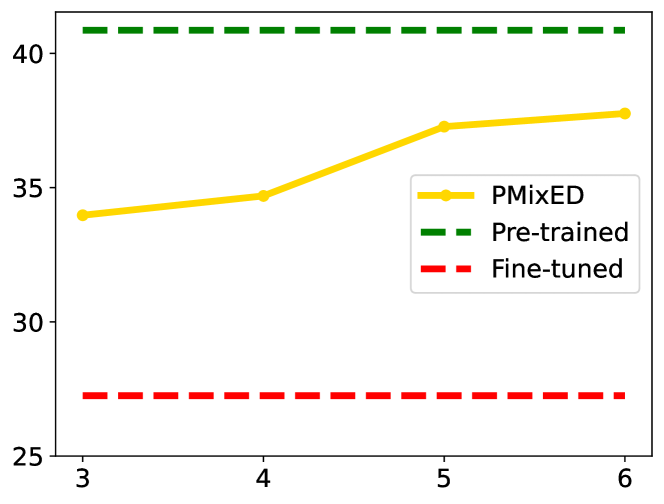
Figure 5: Alpha

Figure 5 shows the utility trade-off of $\alpha$. Hence, it is crucial to the performance of PMixED that $\alpha$ is small due to the monotonicity property of Renyi Divergence.

Appendix E Extended Related Works

Another promising privacy-related notion, machine unlearning, has emerged to reduce memorization by verifiably removing learned information from a data sample without retraining a model from scratch Guo et al. (2019); Bourtoule et al. (2021). Generally speaking, there are two machine unlearning notions: (1) exact unlearning, where the resulting model has completely unlearned a data sample Bourtoule et al. (2021), and (2) approximate unlearning, where a data point has been unlearned to some degree with high probability. It is well-known that differential privacy implies approximate machine unlearning. One recent, orthogonal work explored the use of task vectors to perform memorization unlearning of the private dataset Gao et al. (2024).

References

- Abadi et al. (2016) Martin Abadi, Andy Chu, Ian Goodfellow, H Brendan McMahan, Ilya Mironov, Kunal Talwar, and Li Zhang. 2016. Deep learning with differential privacy. In Proceedings of the 2016 ACM SIGSAC conference on computer and communications security, pages 308–318.
- Balle et al. (2020) Borja Balle, Gilles Barthe, Marco Gaboardi, Justin Hsu, and Tetsuya Sato. 2020. Hypothesis testing interpretations and renyi differential privacy. In International Conference on Artificial Intelligence and Statistics, pages 2496–2506. PMLR.
- Bourtoule et al. (2021) Lucas Bourtoule, Varun Chandrasekaran, Christopher A Choquette-Choo, Hengrui Jia, Adelin Travers, Baiwu Zhang, David Lie, and Nicolas Papernot. 2021. Machine unlearning. In 2021 IEEE Symposium on Security and Privacy (SP), pages 141–159. IEEE.
- Bun and Steinke (2016) Mark Bun and Thomas Steinke. 2016. Concentrated differential privacy: Simplifications, extensions, and lower bounds. In Theory of Cryptography Conference, pages 635–658. Springer.
- Carlini et al. (2019) Nicholas Carlini, Chang Liu, Úlfar Erlingsson, Jernej Kos, and Dawn Song. 2019. The secret sharer: Evaluating and testing unintended memorization in neural networks. In 28th USENIX Security Symposium (USENIX Security 19), pages 267–284.
- Carlini et al. (2021) Nicholas Carlini, Florian Tramer, Eric Wallace, Matthew Jagielski, Ariel Herbert-Voss, Katherine Lee, Adam Roberts, Tom Brown, Dawn Song, Ulfar Erlingsson, et al. 2021. Extracting training data from large language models. In 30th USENIX Security Symposium (USENIX Security 21), pages 2633–2650.
- Chelba et al. (2013) Ciprian Chelba, Tomas Mikolov, Mike Schuster, Qi Ge, Thorsten Brants, Phillipp Koehn, and Tony Robinson. 2013. One billion word benchmark for measuring progress in statistical language modeling. arXiv preprint arXiv:1312.3005.
- Dai et al. (2019) Zihang Dai, Zhilin Yang, Yiming Yang, Jaime Carbonell, Quoc V Le, and Ruslan Salakhutdinov. 2019. Transformer-xl: Attentive language models beyond a fixed-length context. arXiv preprint arXiv:1901.02860.
- Dwork (2006) Cynthia Dwork. 2006. Differential privacy. In International colloquium on automata, languages, and programming, pages 1–12. Springer.
- Dwork and Feldman (2018) Cynthia Dwork and Vitaly Feldman. 2018. Privacy-preserving prediction. In Conference On Learning Theory, pages 1693–1702. PMLR.
- Dwork et al. (2014) Cynthia Dwork, Aaron Roth, et al. 2014. The algorithmic foundations of differential privacy. Foundations and Trends® in Theoretical Computer Science, 9(3–4):211–407.
- EU (2024) EU. 2024. The artificial intelligence act. https://data.consilium.europa.eu/doc/document/ST-5662-2024-INIT/en/pdf.
- Fan et al. (2018) Angela Fan, Mike Lewis, and Yann Dauphin. 2018. Hierarchical neural story generation. arXiv preprint arXiv:1805.04833.
- Gao et al. (2024) Lei Gao, Yue Niu, Tingting Tang, Salman Avestimehr, and Murali Annavaram. 2024. Ethos: Rectifying language models in orthogonal parameter space. arXiv preprint arXiv:2403.08994.
- Ginart et al. (2022) Antonio Ginart, Laurens van der Maaten, James Zou, and Chuan Guo. 2022. Submix: Practical private prediction for large-scale language models. arXiv preprint arXiv:2201.00971.
- Guo et al. (2019) Chuan Guo, Tom Goldstein, Awni Hannun, and Laurens Van Der Maaten. 2019. Certified data removal from machine learning models. arXiv preprint arXiv:1911.03030.
- Holtzman et al. (2019) Ari Holtzman, Jan Buys, Li Du, Maxwell Forbes, and Yejin Choi. 2019. The curious case of neural text degeneration. arXiv preprint arXiv:1904.09751.
- Hu et al. (2021) Edward J Hu, Yelong Shen, Phillip Wallis, Zeyuan Allen-Zhu, Yuanzhi Li, Shean Wang, Lu Wang, and Weizhu Chen. 2021. Lora: Low-rank adaptation of large language models. arXiv preprint arXiv:2106.09685.
- Husain et al. (2020) Hisham Husain, Borja Balle, Zac Cranko, and Richard Nock. 2020. Local differential privacy for sampling. In International Conference on Artificial Intelligence and Statistics, pages 3404–3413. PMLR.
- Jozefowicz et al. (2016) Rafal Jozefowicz, Oriol Vinyals, Mike Schuster, Noam Shazeer, and Yonghui Wu. 2016. Exploring the limits of language modeling. arXiv preprint arXiv:1602.02410.
- Kamath (2020) Gautam Kamath. 2020. Lecture 14– private ml and stats: Modern ml. http://www.gautamkamath.com/CS860notes/lec14.pdf.
- Khandelwal et al. (2019) Urvashi Khandelwal, Omer Levy, Dan Jurafsky, Luke Zettlemoyer, and Mike Lewis. 2019. Generalization through memorization: Nearest neighbor language models. arXiv preprint arXiv:1911.00172.
- Li et al. (2021) Xuechen Li, Florian Tramer, Percy Liang, and Tatsunori Hashimoto. 2021. Large language models can be strong differentially private learners. arXiv preprint arXiv:2110.05679.
- Majmudar et al. (2022) Jimit Majmudar, Christophe Dupuy, Charith Peris, Sami Smaili, Rahul Gupta, and Richard Zemel. 2022. Differentially private decoding in large language models. arXiv preprint arXiv:2205.13621.
- McMahan et al. (2017) H Brendan McMahan, Daniel Ramage, Kunal Talwar, and Li Zhang. 2017. Learning differentially private recurrent language models. arXiv preprint arXiv:1710.06963.
- Merity et al. (2016) Stephen Merity, Caiming Xiong, James Bradbury, and Richard Socher. 2016. Pointer sentinel mixture models. arXiv preprint arXiv:1609.07843.
- Mironov (2017) Ilya Mironov. 2017. Rényi differential privacy. In 2017 IEEE 30th computer security foundations symposium (CSF), pages 263–275. IEEE.
- Nasr et al. (2021) Milad Nasr, Shuang Songi, Abhradeep Thakurta, Nicolas Papernot, and Nicholas Carlin. 2021. Adversary instantiation: Lower bounds for differentially private machine learning. In 2021 IEEE Symposium on security and privacy (SP), pages 866–882. IEEE.
- Nissim et al. (2007) Kobbi Nissim, Sofya Raskhodnikova, and Adam Smith. 2007. Smooth sensitivity and sampling in private data analysis. In Proceedings of the thirty-ninth annual ACM symposium on Theory of computing, pages 75–84.
- Papernot et al. (2016) Nicolas Papernot, Martín Abadi, Ulfar Erlingsson, Ian Goodfellow, and Kunal Talwar. 2016. Semi-supervised knowledge transfer for deep learning from private training data. arXiv preprint arXiv:1610.05755.
- Papernot et al. (2018) Nicolas Papernot, Shuang Song, Ilya Mironov, Ananth Raghunathan, Kunal Talwar, and Úlfar Erlingsson. 2018. Scalable private learning with pate. arXiv preprint arXiv:1802.08908.
- Ponomareva et al. (2023) Natalia Ponomareva, Hussein Hazimeh, Alex Kurakin, Zheng Xu, Carson Denison, H Brendan McMahan, Sergei Vassilvitskii, Steve Chien, and Abhradeep Guha Thakurta. 2023. How to dp-fy ml: A practical guide to machine learning with differential privacy. Journal of Artificial Intelligence Research, 77:1113–1201.
- Radford et al. (2019) Alec Radford, Jeffrey Wu, Rewon Child, David Luan, Dario Amodei, Ilya Sutskever, et al. 2019. Language models are unsupervised multitask learners. OpenAI blog, 1(8):9.
- Redberg et al. (2023) Rachel Redberg, Yuqing Zhu, and Yu-Xiang Wang. 2023. Generalized ptr: User-friendly recipes for data-adaptive algorithms with differential privacy. In International Conference on Artificial Intelligence and Statistics, pages 3977–4005. PMLR.
- Steinke (2022) Thomas Steinke. 2022. Composition of differential privacy & privacy amplification by subsampling. arXiv preprint arXiv:2210.00597.
- US (2023) US. 2023. Safe, secure, and trustworthy development and use of artificial intelligence. https://www.federalregister.gov/documents/2023/11/01/2023-24283/safe-secure-and-trustworthy-development-and-use-of-artificial-intelligence.
- van der Maaten and Hannun (2020) Laurens van der Maaten and Awni Hannun. 2020. The trade-offs of private prediction. arXiv preprint arXiv:2007.05089.
- Wolf et al. (2019) Thomas Wolf, Lysandre Debut, Victor Sanh, Julien Chaumond, Clement Delangue, Anthony Moi, Pierric Cistac, Tim Rault, Rémi Louf, Morgan Funtowicz, et al. 2019. Huggingface’s transformers: State-of-the-art natural language processing. arXiv preprint arXiv:1910.03771.
- Xu et al. (2023) Zheng Xu, Maxwell Collins, Yuxiao Wang, Liviu Panait, Sewoong Oh, Sean Augenstein, Ting Liu, Florian Schroff, and H. Brendan McMahan. 2023. Learning to generate image embeddings with user-level differential privacy. In Proceedings of the IEEE/CVF Conference on Computer Vision and Pattern Recognition (CVPR), pages 7969–7980.
- Yousefpour et al. (2021) Ashkan Yousefpour, Igor Shilov, Alexandre Sablayrolles, Davide Testuggine, Karthik Prasad, Mani Malek, John Nguyen, Sayan Ghosh, Akash Bharadwaj, Jessica Zhao, et al. 2021. Opacus: User-friendly differential privacy library in pytorch. arXiv preprint arXiv:2109.12298.
- Yu et al. (2021) Da Yu, Saurabh Naik, Arturs Backurs, Sivakanth Gopi, Huseyin A Inan, Gautam Kamath, Janardhan Kulkarni, Yin Tat Lee, Andre Manoel, Lukas Wutschitz, et al. 2021. Differentially private fine-tuning of language models. arXiv preprint arXiv:2110.06500.