TAMS: Translation-Assisted Morphological Segmentation

Abstract

Canonical morphological segmentation is the process of analyzing words into the standard (aka underlying) forms of their constituent morphemes. This is a core task in language documentation, and NLP systems have the potential to dramatically speed up this process. But in typical language documentation settings, training data for canonical morpheme segmentation is scarce, making it difficult to train high quality models. However, translation data is often much more abundant, and, in this work, we present a method that attempts to leverage this data in the canonical segmentation task.

We propose a character-level sequence-to-sequence model that incorporates representations of translations obtained from pretrained high-resource monolingual language models as an additional signal. Our model outperforms the baseline in a super-low resource setting but yields mixed results on training splits with more data. While further work is needed to make translations useful in higher-resource settings, our model shows promise in severely resource-constrained settings.

1 Introduction

Morphological segmentation is the task of breaking words into morphemes, the smallest semantic units of a language. Morphemes can merge and change during word formation, and the precise morphological composition of a word is often obfuscated in its surface form. Segmentation can thus take two forms: surface/linear segmentation and canonical segmentation, which divides a word into the “canonical” forms of its morphemes (cf. Figure 1).

One important motivation for automated canonical segmentation is to expedite the process of linguistic analysis, including the creation of Interlinear Glossed Text (IGT). IGT is a form of morphological annotation that typically adheres to the Leipzig glossing format Lehmann (1982), a documentation style wherein each line of the target text is broken up into a transcription line, a gloss line (morphological annotation), and a translation line. IGT is a crucial resource in language documentation work, but it is costly and time-consuming to generate. The task of morphological segmentation is a key component in glossing, and automated canonical segmentation could aid in this process. Prior work has shown that automated methods have the potential to assist language documentation and revitalization Palmer et al. (2009); Moeller et al. (2020); Moeller and Hulden (2021); Chaudhary et al. (2022); Ahumada et al. (2022).

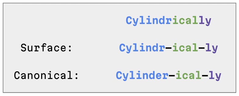
Figure 1: Canonical segmentation of the English word "Cylindrically"

Neural models have been shown to perform well on the task of canonical segmentation (Kann et al., 2016; Ruzsics and Samardžić, 2017), but the success of these models has been restricted by the availability of annotated segmentation data. IGT, though a limited resource, is one important source of training data for canonical segmentation. However, until now, primarily the transcription and gloss lines of IGT have been used as input to segmentation models, while the translations have been overlooked. Moreover, in real-world documentation settings, translated data is often much more available than morphologically analyzed data, making it practically attractive as an additional input. Here we consider how supervised canonical segmentation methods can be improved by leveraging this underutilized data source. Translations also provide the opportunity to make use of pretrained models that likely have much higher-quality representations than any model for the target language.

Our work is inspired in part by Zhao et al. (2020) who experiment with leveraging translations for the task of automatic interlinear glossing. They use a multi-source word-level transformer to jointly model the transcription and translation sequences, and outperform previous baselines. Their work shows promise for the utility of translation data in morphological analysis tasks. However, they assume the presence of well-segmented data and state that "proper segmentation remains a challenge and that the creation of segmentation tools is a valuable endeavor." Our work endeavors to address the segmentation issue.

We treat canonical segmentation as a sequence-to-sequence problem and use a character-level pointer-generator LSTM See et al. (2017) to map each surface form word to its segmented, canonicalized form. We experiment with Tsez and Lezgi, two Northeast Caucasian languages, and Arapaho, a Plains Algonquian language. We leverage existing sentence-level English translations present in the IGT data from the SIGMORPHON 2023 Shared Task on Interlinear Glossing Ginn et al. (2023) and create two datasets of word-level transcription–translation alignments: automatically with awesome-alignDou and Neubig (2021), and manually according to conventions described in §4.3.2. We then embed these translations with BERT Devlin et al. (2019) and experiment with incorporating them into our baseline model’s encoder and decoder. We also analyze the impact of training set size on the efficacy of our approach by limiting our training split to simulate varied levels of resourcedness. Finally, we analyze the effect of automatic vs. manual word-alignments on the subset of the Tsez data that we manually aligned.

We find that our approach is most impactful in the extremely low data setting (n=100) and outperforms the baseline by an average of 2.33% and as high as 3.88% accuracy. However, in the higher data settings, incorporating translations may or may not be beneficial. Our results also suggest that gold aligned data may not be necessary to see improvements over the baseline.

2 Related Work

Modeling Morphological Segmentation

Recent work on neural methods for canonical segmentation primarily focuses on LSTMs. Kann et al. (2016) use a bidirectional RNN encoder-decoder with a neural reranker. Mager et al. (2020) adapt this work to the low-resource setting and find that the pointer-generator network vastly improves over the performance of the LSTM canonical segmentation model for this setting. Recent work has also used the transformer for canonical segmentation: Moeng et al. (2021) test several sequence-to-sequence models for the task and find that the transformer performs the best on 4 Nguni languages.

Morphological Information within Embeddings

Previous work has suggested that distributional similarity is an informative cue for morphology (Yarowsky and Wicentowski, 2000; Schone and Jurafsky, 2001) and static word embeddings encode some morphological information (Musil, 2021; Soricut and Och, 2015). Other work has suggested that BERT embeddings could encode grammatical and morphological information Nastase and Merlo (2023); Jawahar et al. (2019). BERT embeddings have also been used for part-of-speech tagging Tsai et al. (2019); Singh et al. (2021); Mohseni and Tebbifakhr (2019). We aim to leverage the morphological cues intrinsic to pretrained embeddings of English translations to improve our segmentation models.

3 Incorporating Translations into Morphological Segmentation Models

Here, we present our method for using translations as a source of additional signal for morphological analysis. Our method relies on alignments to identify word forms in the translation that are relevant for the target word, and embeddings of words in the translation obtained from a high-resource language model are used to assist in the segmentation of the word. We describe several approaches for turning these embeddings into a fixed-length representation and for incorporating them as input to the segmentation model.

3.1 Encoder–Decoder Networks

The most common architecture for morphological analysis is the neural encoder–decoder architecture with attention Bahdanau et al. (2015). An encoder–decoder network estimates the probability of an output sequence $\mathbf{y}=y_{1},\ldots,y_{T^{\prime}}$ in terms of an input sequence $\mathbf{x}=x_{1},\ldots,x_{T}$ by decomposing the output sequence’s joint probability using the chain rule of probability, where $y_{t}$ is conditioned on all previous output items and some representation of the input sequence $v_{t}$ computed using a function $g$:

$$p(y_{1},\ldots,y_{T^{\prime}})= \ \prod_{t=1}^{T^{\prime}}p(y_{t}|v_{t},y_{1},\ldots,y_{t-1})$$

$$v_{t}= \ \mathrm{g}(\mathbf{x},y_{1},\ldots,y_{t-1})$$

For morphological tasks, this architecture is commonly implemented by treating words as character sequences and using RNNs for the encoder and the decoder. The encoder is responsible for producing representations of $\mathbf{x}$ which are useful for the decoder, and the decoder is responsible for producing conditional probability distributions for making a prediction for $\mathbf{y}$, $\mathbf{\hat{y}}$.

3.2 Translation Assistance

The translations of textual data from low-resource languages are usually written in a high-resource language such as English or Spanish. High-resource languages have very high-quality pretrained language models (PLMs) and therefore rich word representations available to them, and we hypothesize that incorporating this signal into the process of morphological segmentation may be helpful. For example, information from the high-resource language might help the segmenter resolve lexical ambiguities. Here, we propose several related methods for incorporating information from a high-resource translation into an RNN-based encoder–decoder morphological segmenter. For clarity, we will concretely consider a unidirectional LSTM-based encoder, though our approach is trivially applicable to other RNN-based encoder–decoder architectures. We refer to the network’s embedding and hidden dimension sizes as $\mathrm{emb}$ and $\mathrm{hid}$, respectively.

Consider a translated sentence with $X$, $Y$, and $R$. $X=\mathbf{x}_{1},\ldots,\mathbf{x}_{n}$ is a sequence of unsegmented words. $Y=\mathbf{y}_{1},\ldots,\mathbf{y}_{n}$ is the sequence of the corresponding segmented words. $R=\mathbf{r}_{1},\ldots,\mathbf{r}_{m}$ is the sequence of words in the translation. We use a PLM to obtain a dense representation for each translation word, $\mathbf{d}=d_{1},\ldots,d_{m}$. We additionally refer to any sentence-wide representation (such as BERT’s [CLS] token) that the PLM might produce as $d_{0}$. We refer to the PLM’s hidden representation size as $\mathrm{h}_{\mathrm{PLM}}$.

Alignment

A preliminary step is to produce an word-level alignment between source words and translation words like so, where $\mathrm{align}$ represents an aligner’s decision on whether two words are aligned:

$$A=\{\langle\mathbf{x}_{i},\mathbf{r}_{j}\rangle|\mathbf{x}_{i}\in X\wedge\mathbf{r}_{j}\in R\wedge\mathrm{align}(\mathbf{x}_{i},\mathbf{r}_{j})\}$$

Translation Representation

For each word $\mathbf{x}$, we now have some aligned translation word representations $\mathbf{d}_{\mathrm{align}}=d_{a},\ldots,d_{b}$. We next produce $v$, a fixed-length representation of $\mathbf{d}_{\mathrm{align}}$ which will be of length $\mathrm{emb}$. We investigate three different strategies for producing this representation which differ in how they treat the sentence-wide representation $d_{0}$.

For the CLS-None strategy, we discard $d_{0}$ and average pool $\mathbf{d}_{\mathrm{align}}$ before using a model parameter $W_{\mathrm{trans}}\in\mathbb{R}^{\mathrm{h}_{\mathrm{PLM}}\times\mathrm{emb}}$ to project the vector from the hidden size of the PLM to the embedding size of the model:

$$v=\mathrm{avg}(d_{a},\ldots,d_{b})W_{\mathrm{trans}}$$

The CLS-Avg strategy is identical to CLS-None except that $d_{0}$ is included in the average:

$$v=\mathrm{avg}(d_{0},d_{a},\ldots,d_{b})W_{\mathrm{trans}}$$

For the CLS-Concat strategy, we first average the aligned words like in CLS-None, but we introduce two model parameters, $W_{\mathrm{trans}},W_{\mathrm{cls}}\in\mathbb{R}^{h_{\mathrm{PLM}}\times\frac{1}{2}\mathrm{emb}}$, where $W_{\mathrm{trans}}$ is applied to the averaged words and $W_{\mathrm{cls}}$ is applied to $\mathbf{d}_{0}$, and their concatenation is used as the final fixed vector:

$$v_{1} =\mathrm{avg}(d_{a},\ldots,d_{b})W_{\mathrm{trans}}$$

$$v_{2} =d_{0}W_{\mathrm{cls}}$$

$$v =v_{1}\oplus v_{2}$$

Incorporation Strategies

After we have computed $v$, we must somehow incorporate it into the encoder and/or the decoder’s process.

For Concat, we double the model’s input size to $2\times\mathrm{emb}$ and concatenate $v$ to the input embedding at each time step in the LSTM. Concat-Half is identical to Concat, except the model’s input size is held constant, with character embeddings and $v$ sharing the dimensions equally. The model’s character embedding module and $W_{\mathrm{trans}}$ above have their output dimensions halved accordingly. For Init-State, assuming that there is some integer $z$ such that $z\times\mathrm{emb}=\mathrm{hid}$, we initialize the LSTM’s hidden state as $z$ concatenations of $v$ to itself, $\bigoplus_{1}^{z}v$. For Init-Char, we modify the LSTM’s input sequence so that $v$ appears first, as if it were the embedding of a character. All strategies are applicable to either the encoder or the decoder; we experiment with most combinations, except for Init-Char in the decoder.

4 Data

To perform our experiments, we use IGT data from the SIGMORPHON 2023 Shared Task on Interlinear Glossing Ginn et al. (2023) in three languages: Lezgi, Tsez, and Arapaho. All of the data is licensed under CC BY-NC 4.0. Each word in this IGT format has a surface form, a canonical form, morpheme-level glosses, and an English translation for the sentence the word appears in. An example is shown in Figure 2, which also provides a sample of our manual alignment process.

4.1 Languages

We experiment with three languages: Arapaho, Lezgi, and Tsez. All three languages present interesting modeling challenges given the complexity of their morphological processes. In addition, the experiments cover different types of difficult morphology, as the two language families represented are typologically distinct.

4.1.1 Tsez

Tsez [ddo] belongs to the Tsezic subgroup, which is part of the larger Nakh-Daghestanian language family. Its morphology is highly agglutinative and suffixing. Tsez has complex nominal case morphology that allows multiple case suffixes to modify a single word, and there are around 250 possible combinations of these case suffixes. In terms of verbal morphology, Tsez separates verbs into four groups depending on the final segment of the stem, which affects the surface representation of the composite morphemes, including five possible indicative tense-aspect suffixes Comrie and Polinsky . Tsez also has a rich set of converbs that are derived from the verb stem through multi-step morphophonological processes. We consider Tsez to be our development language and conduct all hyperparameter tuning on Tsez.

4.1.2 Lezgi

Lezgi [lez] belongs to the Lezgic branch within the Nakho-Daghestanian language family. Like, Tsez, Lezgi is a highly agglutinative language with a largely suffixing morphology. Lezgi morphology is predominantly inflectional and nouns are inflected for number, case, and localization. There are 18 nominal cases in Lezgi, 14 of which are locative Haspelmath (1993). Morphologically, verb stems are divided into three groups – Masdar, Imperfective, and Aorist stems – which impact the inflectional suffixes they can take on. Three distinct verb forms can be derived from the Masdar stem, nine from the Imperfective, and five from the Aorist Haspelmath (1993). Several additional secondary verbal categories particularly relating to mood can be achieved via suffixing on the verb. Given its close phylogenetic relationship to Tsez, we consider Lezgi to be an in-family test language.

4.1.3 Arapaho

Arapaho [arp] is an Algonquian language that is highly agglutinating and polysynthetic. Noun stems can be inflected for plurality, obviation, vocative, and locative cases through suffixing. Nouns also necessarily belong to either animate or inanimate gender, and gender impacts the surface representation of many inflectional markers. Arapaho nouns also participate in derivational morphology, and modified nouns can be derived from independent nouns or verbs. Arapaho verbal morphology is even more complex. In terms of inflectional morphology, verb stems can be divided into four different classes that each take different markers for person, number, and obviation. Verbs can also be broken up into four different orders– affirmative, non-affirmative, conjunct, and imperative– which also impact the inflectional morphemes. Arapaho derivational verbal morphology is extensive, and unique verb forms can be derived through processes of prefixation, suffixation, denominalization, reduplication, and noun incorporation. We consider Arapaho to be an out-of-family test language.

4.2 Preprocessing

The transcription and translation lines are not always pretokenized in these datasets (e.g., punctuation sometimes appears next to words) and it is necessary to tokenize the data for this reason. We use HuggingFace transformers’ Wolf_Debut_Sanh_Chaumond_Delangue_Moi_Cistac_Rault_Louf_Funtowicz_et BertPreTokenize pretokenizer for this purpose, with some additional processing to make language-specific corrections. (In Arapaho, for example, the apostrophe character ' represents a consonant, and it should not be separated from words it appears in.) After this processing, we verify that there are equal numbers of surface and canonical forms, and we discard any sentences for which this is not true. Finally, we initialize our training instances by finding all unique pairs of surface and canonical forms at the word level and choose one randomly if there is more than one occurrence of it in the corpus. Both surface and canonical forms are NFD normalized. Our full datasets consist of 53800 words in Arapaho, 10952 words in Tsez, and 2060 words in Lezgi. In our experiments, the Arapaho dataset is downsampled to 16666 words in order to bring its size closer to the other two datasets.

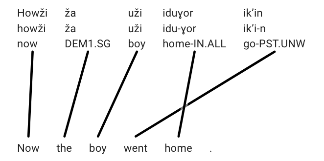
Figure 2: Manual Word Alignment of Tsez IGT: Now the boy went home

4.3 Word Alignment

To facilitate canonical segmentation on the word level, we preprocess our dataset by aligning words in the transcription line to their corresponding word(s) in the translation line. We experiment with two alignment methods: automatic and manual.

4.3.1 Automatic Alignment

We automatically align with awesome-align Dou and Neubig (2021), which extracts word alignments from multilingual BERT and does not require training data for application to a new target language. We use awesome-align’s default hyperparameters except for the following: we use softmax extraction, set the softmax threshold to 5e-6, and set batch size to 32. After alignment, we split the instances for our main experiments into train, development, and test sets at a 60/20/20 ratio.

4.3.2 Manual Alignment

We manually create gold alignments for the Tsez data according to the general principles laid out in Melamed (1998). Melamed (1998) provides conventions for navigating complications that arise when translation is not literal, such as omissions, phrasal correspondence and idioms, amongst other linguistic nuances. Additionally, we define several language-specific principles outlined in Appendix A that address unique difficulties in mapping Tsez grammatical constructions to English. Figure 2 shows an example sentence in Tsez that we have manually aligned. Our full gold-aligned dataset consists of 1419 words, which we divide into 500-word training and test sets, and a 419-word development set.

5 Experiment

We experiment with the strategies described in §3.2 for incorporating information from translations into our morphological segmentation model. We proceed by first tuning our exact approach on the development split of a single language, Tsez, by exhaustively considering every combination of encoder, decoder, and CLS-token translation incorporation strategies. We then apply our top-performing model to the test splits of all three languages. All experiments are performed on NVIDIA A100 GPUs, and all model implementations were based on those provided by Yoyodyne.

5.1 Translation Vectors

We use bert-base-cased Devlin et al. (2019) to generate contextual word embeddings of the translations of each word in our aligned dataset. We then generate fixed-length translation vectors by averaging the embeddings of each word-piece in the translation sequence that was aligned to the word under consideration, as described in §3.

5.2 Evaluation Metrics

We employ three common metrics for evaluation. The first is whole-word accuracy, indicating the proportion of words that were segmented entirely correctly. To get a better picture of subword-level errors, we also use character-level edit distance. Finally, we use the modified F1 score outlined in Mager et al. (2020) to calculate the F1 score at the morpheme level. We consider precision to be the proportion of morphemes in the prediction that also occur in the gold, and recall to be the proportion of morphemes in gold that also occur in the prediction.

5.3 Model and Hyperparameters

In preliminary experiments, we conduct a hyperparameter search in order to determine which model architectures, model sizes, and optimization methods are most effective for these datasets.

Baselines and Settings for Hyperparameter Tuning

Our baseline models for this task perform canonical segmentation without taking translations into account. The architectures we consider are a Transformer, a pointer-generator LSTM with a bidirectional encoder, and an attentive LSTM. Details are outlined in Appendix B. As it would be prohibitively expensive to do this in every experimental setting, we limit the scope of this search to baseline models on the Tsez datasets on three training split sizes: 100, 500, and 6572.

Architectures

The pointer-generator LSTM See et al. (2017) performs better in all settings than either of the two other model architectures, and we therefore adopt it for all subsequent experiments. Moreover, this choice is supported by evidence from Mager et al. (2020) that the pointer-generator is well suited to the low-resource canonical segmentation task.

The pointer-generator LSTM differs from a regular LSTM encoder-decoder in that it has a pointer network Vinyals et al. (2015), which allows the model to copy over specific characters in the input sequence to the output sequence.

The decoder assesses the probability of copying an element from the input to the output rather than generating it, then computes the probability distribution of the output at each time step by combining the probability distribution across the output vocabulary with the attention distribution over the input characters. The weights, indicating the probability of generation or copying, are determined by a feedforward network.

Data Size Matters

The results of hyperparameter tuning are very similar for the 500-sentence and full data settings, but vary notably for the 100-sample setting.

In all subsequent experiments, we train our 100 training sample models with one set of hyperparameters and all other models with a separate set. In the 100-sample setting, we use a batch size of 16, two encoder and two decoder layers, an embedding size of 512 and a hidden size of 1024. We set dropout to $3.662\times 10^{-1}$, learning rate to $2.411\times 10^{-4}$, and train for up to 607 epochs.

For all other experimental settings, we use a batch size of 64, one encoder and one decoder layer, an embedding size of 1024, and a hidden size of 2048. We set dropout to $2.212\times 10^{-1}$, learning rate to $8.056\times 10^{-4}$, and train for up to 627 epochs.

Both settings use the Adam optimizer and the ReduceLROnPlateau scheduler.

Incorporating Translation Information

We treat translation incorporation strategy as a hyperparameter and test all combinations on the Tsez development set to determine the optimal approach.

We take the average whole-word accuracy for configuration across all training split sizes on the Tsez development set using the CLS-None strategy. The full results of this search are shown in Table 1. From this search, we find that the overall highest performing strategy configuration is Init-State in the encoder and Concat-Half in the decoder. This configuration outperforms the baseline by an average of 1.58% and is the top performer on the 100 and 500 train sample settings. Only in the highest train data setting does the baseline outperform our top configuration.

For the 100 train sample setting, Concat in the encoder and Concat-Half in the decoder, the second highest performing configuration overall, was the top configuration. With this in mind, we perform a second search over the CLS strategies on these two configurations, shown in Table 2. From this, we find that the overall highest performing configuration is Init-State in the encoder, Concat-Half in the decoder and CLS-Concat as our CLS Strategy; we call this model TAMS.

Encoder Strat.	Decoder Strat.	n = 100	n = 250	n = 500	n = 6572	Average
Init-State	Concat-Half	22.47	34.02	45.39	80.46	45.58
Concat	Concat-Half	24.66	32.33	45.02	80.09	45.53
Concat-Half	Concat-Half	24.57	32.51	44.20	80.82	45.53
None	Concat-Half	23.56	32.19	44.57	81.10	45.35
Concat	Init-State	23.70	31.46	45.21	80.82	45.30
Concat	Concat	22.92	32.05	44.84	80.55	45.09
Init-State	None	22.60	31.46	44.43	80.91	44.85
None	Concat	23.11	31.23	44.38	80.46	44.79
Concat	None	23.24	30.18	45.21	80.46	44.77
Init-State	Init-State	21.60	31.28	45.21	80.91	44.75
Concat-Half	None	23.01	30.87	43.15	81.32	44.59
None	Init-State	22.15	31.83	43.11	81.00	44.52
Concat-Half	Concat	23.06	31.46	43.01	80.23	44.44
Init-State	Concat	22.51	31.00	43.70	80.50	44.43
Concat-Half	Init-State	22.88	31.42	40.96	81.32	44.14
None	None	22.56	28.90	43.06	81.87	44.10
Init-Char	Concat-Half	24.11	29.54	40.91	79.63	43.55
Init-Char	Concat	21.74	31.23	39.54	79.27	42.95
Init-Char	Init-State	22.33	24.89	41.55	80.09	42.21
Init-Char	None	23.29	22.60	39.36	80.91	41.54

Table 1: Model tuning 1: Accuracy (%) of all translation incorporation strategies on Tsez’s silver-aligned development split with no information from the CLS token (CLS-None).

Encoder Strat.	Decoder Strat.	CLS Strat.	n = 100	n = 250	n = 500	n = 6572	Average
Init-State	Concat-Half	CLS-Concat	23.29	33.79	45.16	80.68	45.73
Init-State	Concat-Half	CLS-None	22.47	34.02	45.39	80.46	45.58
Concat	Concat-Half	CLS-None	24.66	32.33	45.02	80.09	45.53
Concat	Concat-Half	CLS-Avg	23.70	32.42	45.30	80.41	45.46
Init-State	Concat-Half	CLS-Avg	22.79	33.42	45.02	80.55	45.45
Concat	Concat-Half	CLS-Concat	23.20	30.41	46.12	80.32	45.01
None	None	-	22.56	28.90	43.06	81.87	44.10

Table 2: Model tuning 2: Accuracy (%) of CLS strategies with top-performing translation incorporation configurations on the Tsez silver-aligned development split.

6 Results with Final Model Configuration

		Tsez		Lezgi		Arapaho
Train Limit	Metrics	TAMS	Baseline	TAMS	Baseline	TAMS	Baseline
	Accuracy	23.24	22.65	27.91	24.03	12.34	9.82
n = 100	F1	43.31	41.24	41.92	38.32	28.61	23.84
	ED	3861	4065	808	902	37024	37719
	Accuracy	35.39	31.05	33.25	34.71	19.65	18.08
n = 250	F1	57.14	54.74	51.06	53.00	41.36	40.61
	ED	3156	3442	691	715	29022	30344
	Accuracy	44.52	43.11	40.78	41.99	30.59	31.53
n = 500	F1	64.43	63.43	55.66	57.42	51.91	53.02
	ED	2427	2655	636	639	21339	21261
	Accuracy	80.78	82.60	46.84	44.66	67.72	67.08
n = all	F1	89.52	90.44	62.48	60.75	81.62	81.11
	ED	701	652	532	568	9899	10495

Table 3: Final results per language: Performance on all languages’ test sets on silver-aligned data.

Train Limit	TAMS (abs/$\Delta$)	Baseline
n = 100	21.16 (+2.33)	18.83
n = 250	29.43 (+1.48)	27.95
n = 500	38.63 (-0.25)	38.88
Full Train Split	65.11 (+0.33)	64.78

Table 4: Final results, all languages: Average accuracy (%) by training split size across all languages.

Model	Metrics	Gold	Awesome-Gold
	Accuracy	53.60	54.60
TAMS	F1	67.98	67.89
	ED	450	443
Baseline	Accuracy	55.40
	F1	70.19
	ED	435

Table 5: Manual vs. automatic alignment: Performance on Tsez’s gold-aligned test split (n=500).

As described above, we perform search over the Tsez development set to determine the overall highest performing model, which we call TAMS. This configuration consists of Init-State in the encoder, Concat-Half in the decoder, and CLS-Concat as the CLS strategy.

6.1 Test Languages

We apply our final model configuration to the automatically aligned test sets in each of our three languages: Tsez (development language), Lezgi (in-family test language), and Arapaho (out-of-family test language.

Results are shown in Table 3. In most cases, we see that edit distance, F1, and accuracy are in agreement, so we focus on accuracy as our main evaluation metric. We report the average accuracy across languages for each training data setting in Table 4. We find that on average our model outperforms the baseline in every train data setting except for n=500. In general, performance gains are highest on the lower-resource settings, while on the higher-resource settings, performance improvements are slight if present at all. In the n=100 setting, TAMS outperforms the baseline by an average of 2.33%, suggesting that our model is most beneficial in truly low-data settings. Even for Lezgi, the language for which TAMS has the most varied results, on the 100 sample train-split TAMS yields a 3.88% increase in accuracy over the baseline. We also see consistent gains on Arapaho in all data settings except for n=500 which indicates that with further work, our model could be useful for polysynthetic languages. This is particularly exciting considering the relative difficulty of segmenting polysynthetic languages. However, TAMS’ performance on Lezgi is very uneven despite Lezgi’s linguistic similarity to Tsez, which indicates that the exact translation incorporation configuration we use in TAMS may not be fully extensible to other languages even if they are morphologically similar, and one may need to tune the translation strategy to fit their particular data setting.

6.2 Manual vs. Automatic Alignment

We additionally train a TAMS model on gold-aligned Tsez data (Gold) and compare it to a a TAMS model trained on equivalent data aligned with awesome-align (Awesome-Gold). We evaluate on gold-aligned data (note: this data split is distinct from the one in §6.1). We report the performance metrics of each model in Table 5. We find that the TAMS model trained with Awesome-Gold data actually outperforms its Gold counterpart on every metric except for F1. This suggests that gold alignment data might not be necessary to see the best possible performance from TAMS. This is a positive result because automatic alignment is much less costly than expert alignment and makes training a TAMS model more feasible for a broader range of languages. That said, the baseline outperforms both TAMS models, which complicates our analysis. Another potential issue is awesome-align’s use of mBERT, whose performance varies across languages Wu and Dredze (2020). Further work experimenting with different more languages and data resource levels is necessary to be more conclusive about gold vs. automatic alignment.

7 Conclusion

We present a novel method for incorporating information from translations into a morphological segmentation model to support low-resource canonical segmentation. Using Tsez as a development language, we determine our best-performing model (TAMS), which uses a fixed-length representation of the translation in two ways: to initialize the hidden state in the encoder (Init-State) and to concatenate to the input at each time step in the decoder (Concat-Half). Our model is most beneficial in the super low-resource setting (n=100), where it outperforms the baseline by 2.33% on average across three morphologically complex languages. And although we only tune our model on the Tsez development set, we also see impressive performance gains in all but one training split for Arapaho, a typologically and morphologically distinct polysynthetic language. This promising result suggests that TAMS could be beneficial for a wide range of languages. However, our results are more mixed in higher-resource settings which indicates that there is still more work to be done to determine whether translations are a valuable addition to canonical segmentation models in cases where more data is available. Overall, canonical segmentation for morphologically complex languages remains a challenging task, but we believe that this work indicates that translations should be explored further as an additional data resource.

There are several avenues for future work we wish to highlight. A first possible improvement strategy could be to experiment with providing more explicit information instead of or in addition to translations, such as the POS tags of the aligned English words. Second, it would be interesting to see whether our results can be reproduced on other languages and with other PLMs. Third, there may be other ways to use translation-based representations with LSTMs.

Limitations

Due to data availability, we experimented only on two language families, Northeast Caucasian and Algonquian, but ideally we would have tested on more language families. We cannot concretely say that our models would perform equivalently on a more diverse set of languages. Another limitation was in the exhaustiveness of our hyperparameter search. Ideally, we would have searched each possible CLS-token strategy with each possible configuration of translation incorporation strategies but we were unable to due to the GPU hours that would have been required.

8 Acknowledgements

Thanks to Bernard Comrie for helping us out with the Tsez dataset.

Appendix A Manual Word Alignment Directives

A.1 High-level Directives

• Align English prepositions with the Tsez word with the equivalent case marker

• If some grammatical information is expressed in one language but not the other, behave as if it were expressed in the corresponding phrase. In such cases, the extra word (the, for example) should be aligned to the head of the corresponding phrase.

• But, if the definiteness is expressed on a modifier of the noun head (like an attributive adjective), then align the article to the modifier bearing the definiteness information instead.

A.2 Lower-level Directives

• Pronominal subjects that are not expressed in Tsez and are expressed in English should have the English subject aligned to the head predicate in Tsez

• If in English you have a PP and in Tsez you have a relative clause where the subject position has the gap, align the preposition introducing the PP with the relative clause’s predicate

• If a quotative verb like “say” is used a variable amount of times in one language compared to the other, then align all instances of the quotative verbs together, so long as the quoted material they’re all referring to is identical.

• Always align the expletive there with the existential verb in Tsez. And if there is an adverbial there-equivalent in Tsez, do not align it with anything in English unless there really is an adverbial, non-expletive there or similar in English

• For articles in English, if there’s something very close to an article in Tsez (‘a’, or ‘this’, or …), then prefer aligning the English article to the similar word instead of the noun.

Appendix B Hyperparameter Tuning

We conduct hyperparameter tuning for the baseline Tsez models without translation using random search with the full training set of 6572. We then took the top two architectures and performed a hyper-parameter sweep with 100 and 500 training samples to simulate a lower-resource setting. The top performing models for each architecture and training set size are outlined in Tables 8, 7, 6. The search space of architecture specific hyperparameters is outlined in Table 9 and Table 10 and the search space of optimization parameters is outlined in Table 11. All models used Adam optimization. We report whole-word accuracy on the development set.

Table 6: Best Performing Hyperparameters for Each Architecture with 6572 Training Samples

Hyperparameter	Transformer	Pointer-Generator LSTM	Attentive LSTM
Embedding Size	512	896	512
Hidden Size	1024	1856	960
Dropout	0.3022	0.2212	0.07615
Attention Heads	8	1	1
Encoder Layers	4	1	2
Decoder Layers	2	1	1
Batch Size	16	64	128
Learning Rate (LR)	0.0001975	0.0008056	0.0002227
Beta1	0.8153	0.8218	0.841
Beta2	0.9874	0.9845	0.9815
Scheduler	reduceonplateau	reduceonplateau	None
Num Warmup Samples	-	-	-
Reduce LR Factor	0.3095	0.782	-
Reduce LR Patience	40	30	-
Min LR	0.3095	0.0007737	-
Accuracy	0.8629	0.8634	0.8645

Table 7: Best Performing Hyperparameters for Each Architecture with 500 Training Samples

Hyperparameter	Pointer-Generator LSTM	Attentive LSTM
Embedding Size	320	320
Hidden Size	1728	2048
Dropout	0.3915	0.4794
Attention Heads	1	1
Encoder Layers	1	2
Decoder Layers	1	1
Batch Size	64	16
Learning Rate	0.0007847	0.00008051
Beta1	0.8699	0.8789
Beta2	0.9803	0.9971
Scheduler	-	-
Num Warmup Samples	-	-
Reduce LR Factor	-	-
Reduce LR Patience	-	-
Min LR	-	-
Accuracy	0.5059	0.5059

Table 8: Best Performing Hyperparameters for Each Architecture with 100 Training Samples

Hyperparameter	Pointer-Generator LSTM	Attentive LSTM
Embedding Size	640	192
Hidden Size	896	384
Dropout	0.3662	0.3132
Attention Heads	1	1
Encoder Layers	2	1
Decoder Layers	2	1
Batch Size	16	16
Learning Rate	0.0002411	0.0000523
Beta1	0.8716	0.8263
Beta2	0.9848	0.9875
Scheduler	’reduceonplateau’	-
Num Warmup Samples	-	-
Reduce LR Factor	0.686	-
Reduce LR Patience	30	-
Min LR	0.0005021	-
Accuracy	0.2409	0.157

Table 9: Architecture Hyperparameters Search Space

Hyperparameter	Distribution	Minimum	Maximum
Embedding Size	q_uniform	128	1024
Hidden Size	q_uniform	128	2048
Dropout	uniform	0	0.5

Table 10: Conditional Hyperparameters based on Architecture Type

Model	Attention Heads	Number of Encoder Layers	Number of Decoder Layers
Transformer	[2, 4, 8]	[2, 4, 6, 8]	[2, 4, 6, 8]
Pointer-Generator LSTM	[1]	[1, 2]	[1, 2]
Attentive LSTM	[1]	[1, 2]	[1, 2]

Table 11: Optimization Hyperparameters Search Space

Hyperparameter	Distribution	Values
Batch Size	categorical	[16, 32, 64]
Learning Rate	log_uniform_values	$1\times 10^{-6}$ to 0.01
Beta1	uniform	0.8 to 0.999
Beta2	uniform	0.98 to 0.999
Scheduler	values	[’reduceonplateau’, ’warmupinvsqrt’, None]
Num Warmup Samples	q_uniform	0 to 5000000
Reduce LR Factor	uniform	0.1 to 0.9
Reduce LR Patience	q_uniform	10 to 50
Min LR	uniform	$1\times 10^{-7}$ to 0.001

References

- Ahumada et al. (2022) Cristian Ahumada, Claudio Gutierrez, and Antonios Anastasopoulos. 2022. Educational tools for mapuzugun. In Proceedings of the 17th Workshop on Innovative Use of NLP for Building Educational Applications (BEA 2022), pages 183–196, Seattle, Washington. Association for Computational Linguistics.
- Bahdanau et al. (2015) Dzmitry Bahdanau, Kyunghyun Cho, and Yoshua Bengio. 2015. Neural machine translation by jointly learning to align and translate. In ICLR.
- Chaudhary et al. (2022) Aditi Chaudhary, Zaid Sheikh, David R Mortensen, Antonios Anastasopoulos, and Graham Neubig. 2022. Autolex: An automatic framework for linguistic exploration.
- (4) Bernard Comrie and Maria Polinsky. Tsez. Unpublished manuscript.
- Devlin et al. (2019) Jacob Devlin, Ming-Wei Chang, Kenton Lee, and Kristina Toutanova. 2019. Bert: Pre-training of deep bidirectional transformers for language understanding. In Proceedings of the 2019 Conference of the North American Chapter of the Association for Computational Linguistics: Human Language Technologies, Volume 1 (Long and Short Papers), page 4171–4186, Minneapolis, Minnesota. Association for Computational Linguistics.
- Dou and Neubig (2021) Zi-Yi Dou and Graham Neubig. 2021. Word alignment by fine-tuning embeddings on parallel corpora. In Proceedings of the 16th Conference of the European Chapter of the Association for Computational Linguistics: Main Volume, page 2112–2128, Online. Association for Computational Linguistics.
- Ginn et al. (2023) Michael Ginn, Sarah Moeller, Alexis Palmer, Anna Stacey, Garrett Nicolai, Mans Hulden, and Miikka Silfverberg. 2023. Findings of the sigmorphon 2023 shared task on interlinear glossing. In Proceedings of the 20th SIGMORPHON workshop on Computational Research in Phonetics, Phonology, and Morphology, page 186–201, Toronto, Canada. Association for Computational Linguistics.
- Haspelmath (1993) Martin Haspelmath. 1993. A grammar of Lezgian. Mouton de Gruyter.
- Jawahar et al. (2019) Ganesh Jawahar, Benoît Sagot, and Djamé Seddah. 2019. What does BERT learn about the structure of language? In Proceedings of the 57th Annual Meeting of the Association for Computational Linguistics, pages 3651–3657, Florence, Italy. Association for Computational Linguistics.
- Kann et al. (2016) Katharina Kann, Ryan Cotterell, and Hinrich Schütze. 2016. Neural morphological analysis: Encoding-decoding canonical segments. In Proceedings of the 2016 Conference on Empirical Methods in Natural Language Processing, page 961–967, Austin, Texas. Association for Computational Linguistics.
- Lehmann (1982) Christian Lehmann. 1982. Directions for interlinear morphemic translations. 16(1–4):199–224.
- Mager et al. (2020) Manuel Mager, Özlem Çetinoğlu, and Katharina Kann. 2020. Tackling the low-resource challenge for canonical segmentation. In Proceedings of the 2020 Conference on Empirical Methods in Natural Language Processing (EMNLP), page 5237–5250, Online. Association for Computational Linguistics.
- Melamed (1998) I. Dan Melamed. 1998. Annotation style guide for the blinker project. (arXiv:cmp-lg/9805004). ArXiv:cmp-lg/9805004.
- Moeller and Hulden (2021) Sarah Moeller and Mans Hulden. 2021. Integrating automated segmentation and glossing into documentary and descriptive linguistics. In Proceedings of the 4th Workshop on the Use of Computational Methods in the Study of Endangered Languages Volume 1 (Papers), pages 86–95, Online. Association for Computational Linguistics.
- Moeller et al. (2020) Sarah Moeller, Ling Liu, Changbing Yang, Katharina Kann, and Mans Hulden. 2020. IGT2P: From interlinear glossed texts to paradigms. In Proceedings of the 2020 Conference on Empirical Methods in Natural Language Processing (EMNLP), pages 5251–5262, Online. Association for Computational Linguistics.
- Moeng et al. (2021) Tumi Moeng, Sheldon Reay, Aaron Daniels, and Jan Buys. 2021. Canonical and Surface Morphological Segmentation for Nguni Languages.
- Mohseni and Tebbifakhr (2019) Mahdi Mohseni and Amirhossein Tebbifakhr. 2019. Morphobert: a persian ner system with bert and morphological analysis. In Proceedings of the First International Workshop on NLP Solutions for Under Resourced Languages (NSURL 2019) co-located with ICNLSP 2019 - Short Papers, page 23–30, Trento, Italy. Association for Computational Linguistics.
- Musil (2021) Tomáš Musil. 2021. Representations of meaning in neural networks for NLP: a thesis proposal. In Proceedings of the 2021 Conference of the North American Chapter of the Association for Computational Linguistics: Student Research Workshop, pages 24–31, Online. Association for Computational Linguistics.
- Nastase and Merlo (2023) Vivi Nastase and Paola Merlo. 2023. Grammatical information in BERT sentence embeddings as two-dimensional arrays. In Proceedings of the 8th Workshop on Representation Learning for NLP (RepL4NLP 2023), pages 22–39, Toronto, Canada. Association for Computational Linguistics.
- Palmer et al. (2009) Alexis Palmer, Taesun Moon, and Jason Baldridge. 2009. Evaluating automation strategies in language documentation. In Proceedings of the NAACL HLT 2009 Workshop on Active Learning for Natural Language Processing, page 36–44, Boulder, Colorado. Association for Computational Linguistics.
- Ruzsics and Samardžić (2017) Tatyana Ruzsics and Tanja Samardžić. 2017. Neural sequence-to-sequence learning of internal word structure. In Proceedings of the 21st Conference on Computational Natural Language Learning (CoNLL 2017), pages 184–194, Vancouver, Canada. Association for Computational Linguistics.
- Schone and Jurafsky (2001) Patrick Schone and Daniel Jurafsky. 2001. Knowledge-free induction of inflectional morphologies. In Second Meeting of the North American Chapter of the Association for Computational Linguistics.
- See et al. (2017) Abigail See, Peter J. Liu, and Christopher D. Manning. 2017. Get to the point: Summarization with pointer-generator networks. In Proceedings of the 55th Annual Meeting of the Association for Computational Linguistics (Volume 1: Long Papers), pages 1073–1083, Vancouver, Canada. Association for Computational Linguistics.
- Singh et al. (2021) Pranaydeep Singh, Gorik Rutten, and Els Lefever. 2021. A pilot study for BERT language modelling and morphological analysis for ancient and medieval Greek. In Proceedings of the 5th Joint SIGHUM Workshop on Computational Linguistics for Cultural Heritage, Social Sciences, Humanities and Literature, pages 128–137, Punta Cana, Dominican Republic (online). Association for Computational Linguistics.
- Soricut and Och (2015) Radu Soricut and Franz Och. 2015. Unsupervised morphology induction using word embeddings. In Proceedings of the 2015 Conference of the North American Chapter of the Association for Computational Linguistics: Human Language Technologies, pages 1627–1637, Denver, Colorado. Association for Computational Linguistics.
- Tsai et al. (2019) Henry Tsai, Jason Riesa, Melvin Johnson, Naveen Arivazhagan, Xin Li, and Amelia Archer. 2019. Small and practical BERT models for sequence labeling. In Proceedings of the 2019 Conference on Empirical Methods in Natural Language Processing and the 9th International Joint Conference on Natural Language Processing (EMNLP-IJCNLP), pages 3632–3636, Hong Kong, China. Association for Computational Linguistics.
- Vinyals et al. (2015) Oriol Vinyals, Meire Fortunato, and Navdeep Jaitly. 2015. Pointer networks. In Advances in Neural Information Processing Systems, volume 28. Curran Associates, Inc.
- Wu and Dredze (2020) Shijie Wu and Mark Dredze. 2020. Are all languages created equal in multilingual bert? In Proceedings of the 5th Workshop on Representation Learning for NLP, page 120–130, Online. Association for Computational Linguistics.
- Yarowsky and Wicentowski (2000) David Yarowsky and Richard Wicentowski. 2000. Minimally supervised morphological analysis by multimodal alignment. In Proceedings of the 38th Annual Meeting of the Association for Computational Linguistics, pages 207–216, Hong Kong. Association for Computational Linguistics.
- Zhao et al. (2020) Xingyuan Zhao, Satoru Ozaki, Antonios Anastasopoulos, Graham Neubig, and Lori Levin. 2020. Automatic interlinear glossing for under-resourced languages leveraging translations. In Proceedings of the 28th International Conference on Computational Linguistics, page 5397–5408, Barcelona, Spain (Online). International Committee on Computational Linguistics.