(eccv) Package eccv Warning: Package ‘hyperref’ is loaded with option ‘pagebackref’, which is *not* recommended for camera-ready version

Supplementary Materials for
Hyperspectral Neural Radiance Fields

Qualitative Results Website

Please also refer to https://hyperspectral-nerf.github.io/supplemental-results-webpage for qualitative results.

1 Introduction

In this work, we demonstrated that Neural Radiance Fields (NeRFs) can be naturally extended to hyperspectral data and are a well-suited tool for hyperspectral 3D reconstruction. The implementation details provided in this supplemental document describe our simple approach to hyperspectral NeRF, but we anticipate future works by the community will improve upon our baseline implementation using our to-be-published dataset, future larger datasets, additional architecture and hyperparameter tuning, and recent advances in NeRFs.

Our full code will be made publicly available for the camera ready version.

2 Implementation Details

We build upon nerfstudio’s nerfacto implementation, from commit ef9e00e. Our code will be made publicly available for the camera ready paper. The original nerfacto pipeline and field are shown in Figs. 1 and 2 respectively.

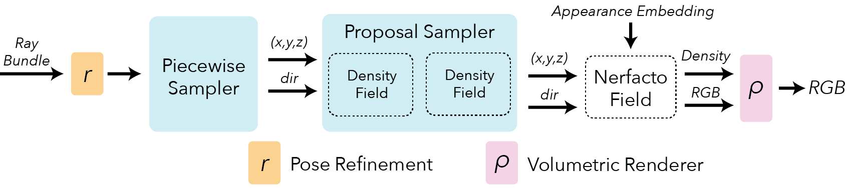
Figure 1: The original nerfacto pipeline (from nerfstudio docs) contains a proposal sampler, which is analagous to the “coarse” field from the original NeRF paper [2], and a “Nerfacto Field”, which is analagous to the primary network from the original NeRF paper ($F_{\Theta}$).

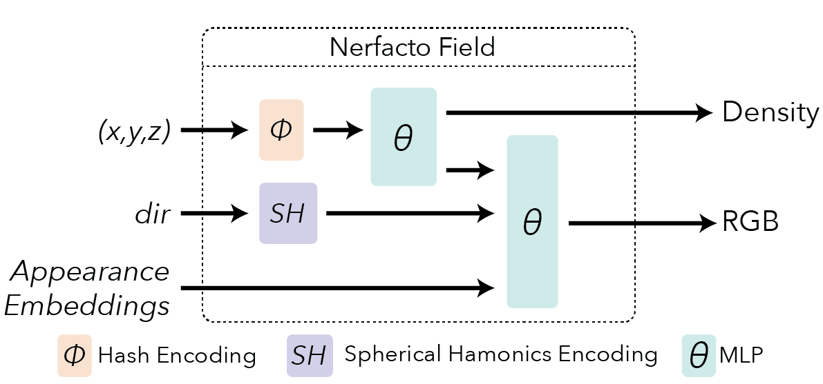
Figure 2: The original nerfacto field (from nerfstudio docs) is very similar to the original NeRF paper [2], but includes appearance embeddings [1] and uses slightly different encodings for the position and direction. This figure is reproduced in Fig. 2 of our main paper.

As briefly summarized in the main paper, we make relatively minimal modifications to the pipeline and field. Using the notation from Section 5.4: Ablations, $\bm{C}_{1}$ only changes the rightmost MLP in Fig. 2 to output 128 channels in the last layer instead of 3; $\bm{C}_{2}$ changes the positional hash encoding ($\phi$ in Fig. 2) to take 4 inputs instead of 3 (appending $\lambda$) and changes the rightmost MLP to only have 1 output for $c$ instead of $(r,g,b)$; and $\bm{C}$ is shown in Fig. 2 (bottom) of the main paper. For $\bm{C}$, the sinusoidal encoding for $\lambda$ is taken to have 8 terms (tested 2, 4, 8, 16 terms, with 8 performing marginally better than 4 and 16, and 2 significantly worse). Also for $\bm{C}$, the component $\bm{C}(\lambda;\Theta_{C})$ MLP from Fig. 2 of the main paper was taken to be identical to the rightmost MLP in Fig. 2 except with the appropriate additional number of inputs to accommodate concatenating the sinusoidally encoded wavelength, and with only 1 output for $c$ instead of 3 for $(r,g,b)$. The latent vector $\Theta_{C}$ was taken to be the same size as in the nerfacto implementation (15-dim), with increasing the size to 32 and 64 showing negligible performance improvement but increased training instability.

Similarly, $\sigma_{0}$ is the stock nerfacto field (scalar); $\sigma_{1}$ only changes the left MLP in Fig. 2 to have 128 outputs; $\sigma_{2}$ changes the positional hash encoding to take 4 inputs, and $\sigma$ is as shown in Fig. 2 (bottom) of the main paper. The additional component $\sigma(\lambda;\Theta_{C})$ MLP has 3 layers with 64-dim hidden layers and ReLU activations. The sinusoidally encoded $\lambda$ is shared with $\bm{C}$ and the latent $\Theta_{\sigma}$ vector is shared with (identical to) the $\Theta_{C}$ vector.

Finally, $P_{0}$ is the stock nerfacto proposal network while $P_{\lambda}$ augments the proposal network with the wavelength. For $P_{\lambda}$, the position is first run through a hash encoding and MLP as in $P_{0}$, except the MLP outputs a latent vector of dimension 7 instead of a scalar density. This latent vector is concatenated with a 2-term sinusoidally encoded wavelength and fed through a 2-layer network with 7-dim hidden layer to output a scalar density for inverse transform ray sampling. Like the original nerfacto pipeline, this sampling step occurs twice with identical architecture (but different weights) proposal networks.

Reiterating our implementation, our primary HS-NeRF implementation uses $\bm{C}(\lambda;\Theta_{C})$, $\sigma_{0}(\lambda;\Theta_{\sigma})$, and $P_{0}$, which we find to produce good results while also enabling wavelength interpolation.

2.1 RGB Implementations

Pseudo-RGB wavelengths.

For the purposes of generating pseudo-RGB images, on the Surface Optics datasets we use the wavelengths 622nm, 555nm, and 503nm for R, G, and B channels respectively.

For the BaySpec datasets, we use a slightly more involved approach. We found that the BaySpec datasets were more sensitive to noise saturation and white balance, so we use an approach similar to that described in Section 6.2 of the main paper to generate pseudo-RGB images. Specifically, we first manually identify 5-10 point correspondences between a hyperspectral image and an iPhone photo of the same scene to represent pairs of colors that should be the same. Expressing the $n$ points in the hyperspectral image as $X\in\mathbb{R}^{128\times n}$ and in the iPhone photo as $Y\in\mathbb{R}^{3\times n}$, we solve for a linear transformation $A\in\mathbb{R}^{3\times 128}=\arg\min_{A^{\prime}}\left\lVert Y-A^{\prime}X\right\rVert^{2}$ using the least squares solution. We then use this transformation to convert the hyperspectral image to pseudo-RGB. After using this initial approach to boot-strap certain components of the pipeline, we later apply the method described in Section 6.2 to generate pseudo-RGB renderings.

HS-NeRF RGB variation implementations.

For the purposes of making a quantitative comparison to standard RGB NeRF, Section 5.2 and Table 1 of the main paper present variations of our approach applied to just 3-channel (RGB) images instead of the full 128-channel hyperspectral data. As described in the caption of Table 1, “Ours-Cont” refers to our HS-NeRF implementation but trained on only 3 wavelengths (so we maintain a continuous representation for radiance spectra, but have very weak supervision of only 3 channels), “Ours-RGB” refers to $\bm{C}_{1},\sigma_{1},P_{0}$ with 3 output channels for both $\bm{C}_{1}$ and $\sigma_{1}$, and “Ours-Hyper” refers to our HS-NeRF implementation trained on all 128 wavelengths. In the table for Ours-Hyper, PSNR and SSIM are evaluated over all 128 wavelengths while LPIPS is evaluated on the RGB images obtained using the Pseudo-RGB procedure.

3 Training Details

All networks were trained for 25000 steps, with 4096 train rays per step using the Adam optimizer. The proposal networks and field both used lr=1e-2, eps=1e-15, and an exponential decay lr schedule to 1e-4 after 20000 steps. Camera extrinsic and intrinsic optimization were both turned off, since evaluation metrics are skewed if camera parameters are modified. To accommodate imperfect camera poses, after COLMAP, stock nerfacto was run on Pseudo-RGB images for 100000 steps with camera optimization turned on and the resulting camera pose corrections were saved and used in subsequent tests. The Surface Optics datasets took roughly 20 minutes to train HS-NeRF while the BaySpec datasets took roughly 40 minutes to train on an RTX 3090 due to the need to re-cache a new set of 32 images every 50 steps (see next paragraph). Most architectures required similar training times, with the exception of the last two rows of the ablation: $\bm{C}_{2}\sigma_{2}P_{0}$ and $\bm{C}\sigma P_{\lambda}$ took at roughly three times as long.

For the Surface Optics datasets, of the 48 images per image set, 43 were used for training and 5 withheld for evaluation. Each step, the 4096 training rays were sampled randomly from all 43 training images, except for row 6 of the ablations where the training rays were sampled from only 10 of the 43 training images each step, with the choice of 10 images being re-sampled every 50 steps. The BaySpec datasets were too large to fit in VRAM so rays were sampled from 32 images every step, with the set of 32 images being re-sampled every 50 steps, with row 6 of the ablations being reduced to 12 images resampled every 50 steps.

In some approaches, not all wavelengths could be run for every step due to VRAM limits so a subset of wavelengths were sampled (randomly) for each step, but every sampled wavelength was run for every ray in the step. For rows 1 and 2 of the ablations, every wavelength could be run every step. For rows 3, 4 (HS-NeRF, ours), and 5, the number of wavelengths sampled per step were 8, 12, and 6, respectively.

For evaluation, every wavelength of every pixel of the 5 (Surface Optics) or 35 (BaySpec) evaluation images were evaluated and compared for each scene.

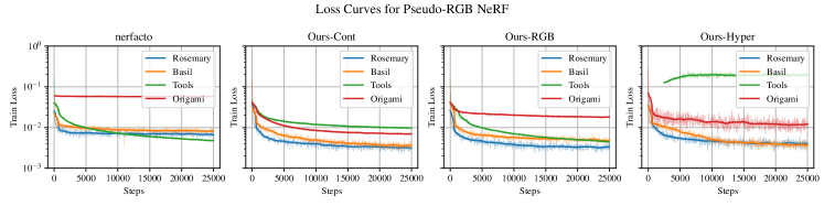
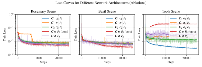
Figure 3: Loss curves for RGB NeRF correspond to the metrics from Table 1 in the main paper. Most scenes have converged by 25000 steps except the Tools scene which appears to have difficulty converging for all methods except “Ours-Cont”

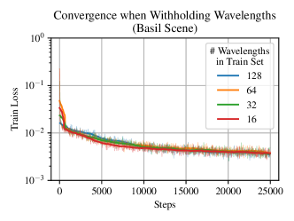
Figure 4: Loss curves for ablation testing (analagous to Table 3 in the main paper) shows that while the rosemary and basil scenes optimize well, the tools scene does not converge particularly well for any method, re-emphasizing the suspected pre-processing (COLMAP) inaccuracy.

Figure 5: Loss curves for HS-NeRF trained with a subset of wavelengths (analogous to Table 2 in the main paper) shows that even training with only 1 out of every 8 wavelengths still has almost identical convergence rate w.r.t. number of steps.

3.1 Commentary on the Tools Scene

The Tools scene experienced instabilities during training with several approaches including both HS-NeRF (ours) and nerfacto (RGB baseline). We anticipate that obtaining better camera intrinsics and extrinsics may correct this issue, since (a) every method had difficulty on this scene and (b) enabling camera pose optimization during NeRF training improved convergence for all methods. Better camera intrinsics could be obtained by initializing COLMAP with the intrinsics obtained from other scenes, and better camera extrinsics could be obtained through a combination of tuning COLMAP parameters, utilizing turntable priors, and a longer NeRF-based camera pose refinement as described in 3. The poor convergence on the Tools scene for all methods is illustrated in both Fig. 5 (green curves) and Fig. 5.

3.2 Loss Curves

To demonstrate that all methods were fairly trained until convergence, the loss curves corresponding to some metrics given in the main paper are shown. As mentioned, the Tools scene appears to have difficulty converging for all methods including baseline nerfacto, suggesting possible pre-processing (COLMAP) inaccuracy. This is evident both in the green curves of Fig. 5 and in the rightmost plot of Fig. 5. Evidencing the hyperspectral super-resolution (spectral interpolation) application, Fig. 5 shows almost identical training loss for all subsets of wavelengths trained with.

4 Qualitative Example Results

A selection of example images and videos with brief explanations are provided at https://hyperspectral-nerf.github.io/supplemental-results-webpage to better gauge our results qualitatively.

References

- [1] Ricardo Martin-Brualla, Noha Radwan, Mehdi S. M. Sajjadi, Jonathan T. Barron, Alexey Dosovitskiy, and Daniel Duckworth. NeRF in the Wild: Neural Radiance Fields for Unconstrained Photo Collections. In CVPR, 2021.
- [2] Ben Mildenhall, Pratul P. Srinivasan, Matthew Tancik, Jonathan T. Barron, Ravi Ramamoorthi, and Ren Ng. Nerf: Representing scenes as neural radiance fields for view synthesis. In ECCV, 2020.