Accuracy Assessment of Discontinuous Galerkin Spectral Element Method in Simulating Supersonic Free Jets

Abstract

The study performs large-eddy simulations of supersonic free jet flows using the Discontinuous Galerkin Spectral Element Method (DGSEM). The main objective of the present work is to assess the resolution requirements for adequate simulation of such flows with the DGSEM approach. The study looked at the influence of the mesh and the spatial discretization accuracy on the simulation results. The present analysis involves four simulations, incorporating three different numerical meshes and two different orders of spatial discretization accuracy. The numerical meshes are generated with distinct mesh topologies and refinement levels. Detailed descriptions of the grid generation and refinement procedures are presented. The study compares flow property profiles and power spectral densities of velocity components with experimental data. The results show a consistent improvement in the computed data as the simulation resolution increases. This investigation revealed a trade-off between mesh and polynomial refinement, striking a balance between computational cost and the accuracy of large-eddy simulation results for turbulent flow analyses.

1 Introduction

Free jet flows exist in many industrial applications, including aerospace engineering, heat transfer, and metalworking. In aerospace engineering, for example, the jet flows are the main responsible for generating thrust from small jet aircraft to large launch vehicles. In the operation of jet flows, the interaction of the high-velocity flow of the jet with the ambient air generates a highly turbulent flow, which induces high levels of pressure fluctuations, responsible for the production of noise and structural loads. The development of the next generation of vehicles and engines requires high-fidelity information on the jet flows in the early stages of the design process to achieve the performance requirements and allow the right design of the structures in the surroundings of the flow. The assessment of the characteristics of the jet flows can be obtained from a test bench in physical experiments [1, 2, 3] and employing numerical simulations [4, 5, 6, 7, 8].

The choice of the approach to obtain a particular characteristic depends on the analysis to be performed. Mean properties, such as thrust and mean velocity field, can be obtained with Reynolds-Averaged Navier-Stokes (RANS) simulations[9], while determining velocity and pressure fluctuations, to estimate the noise produced by the jet at takeoff, demand more sophisticated numerical formulations or the realization of physical experiments. The present work is aligned with the efforts of academia to produce high-fidelity numerical methodologies for the simulation of supersonic jet flows. The large-eddy simulations (LES), which are based on the scale separation of the flow, is the methodology chosen due to its capacity to provide high-frequency flow field information with lower costs when compared to the direct numerical simulation (DNS)[10] or the realization of physical experiments. The use of large-eddy simulations to solve jet flows started some decades ago[11, 12]. The limited availability of computational resources restricted the complexity of the geometries and the Reynolds number that could be resolved. The majority of the simulations were resolving subsonic regimes with the nozzle absent from the computational domain or presented with a simplified geometry. The increase in computational resources allowed the development of simulations with higher Reynolds number flows and more complex geometries [13, 14, 15, 16].

The influence of nozzle-exit conditions was analyzed with the imposition of different boundary layer profiles[4], with a tripped boundary condition[12] and with a highly disturbed boundary layer[17]. The simulations employed a high-order finite difference method to solve the subsonic jet flows with the nozzle represented by a constant radius pipe. The flow field and noise generated by subsonic jet flows were investigated using a compact high-order finite difference method on unstructured meshes[18]. Subsonic heated jet flows were simulated through a high-order framework with a central difference scheme on structured meshes[5] to investigate turbulent temperature fluctuations and heat flux. Multiple strategies to develop the flow inside the nozzle to improve the nozzle outlet condition for a subsonic jet flow were investigated using a finite volume framework on unstructured meshes[19]. High-order frameworks using discontinuous Galerkin have been used to simulate subsonic jet flows[20, 21] in order to perform acoustic analyses. Diverse options of numerical methods have proven capable of simulating subsonic jet flows with accurate flow fields and noise predictions.

The employment of large-eddy simulations for analyzing supersonic jets is less diverse than the subsonic applications. The noise generated by supersonic jet flows has been simulated with finite volume methods on unstructured grids[22, 6, 23]. The acoustic characteristics of supersonic jet flows have also been simulated with finite difference methods[24]. The finite difference method has also been examined to identify the effect of the choice of subgrid-scale (SGS) models[25] on the results of the LES of supersonic jet flow. More recently, simulations using the discontinuous Galerkin schemes are being employed to predict the noise generated by supersonic jet flows[26, 27].

In the present work, a numerical investigation is performed to assess the accuracy of the discontinuous Galerkin spectral element method (DGSEM)[28, 29] in the simulation of supersonic jet flows. For visual representation purposes, Fig. 1 presents 2-D cuts of the supersonic flow assessed in the article, depicting velocity contours and Q-criterion isosurfaces colored by vorticity magnitude over pressure contours in grayscale in the background. The presence of shock waves and the possible need to model the jet nozzle introduces additional challenges to the simulation of a supersonic jet flows compared to subsonic cases. The DGSEM scheme is a high-order framework on unstructured meshes with enhanced computational efficiency obtained by collocating the interpolation and integration points and using a tensor product nodal basis functions inside the hexahedron elements. In the present effort, the version of the DGSEM approach, as implemented in the open-source FLEXI numerical framework[30], is used. The numerical investigation comprises three numerical meshes with two topologies and two polynomial degrees for the spatial discretization in order to identify the mesh and polynomial hp refinement requirements to obtain high-quality results with the numerical scheme.

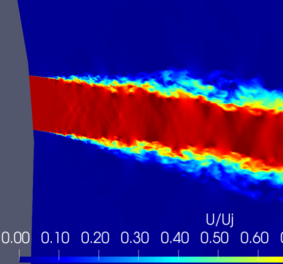
(a) Velocity contours.

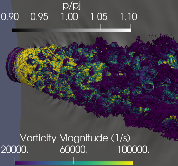
(b) Pressure contours with isosurfaces of Q-criterion colored by vorticity magnitude.

Figure 1: Visualization of the jet flow of interest in the present work.

This work is organized with the governing equations of the LES simulations and the numerical formulation of the discontinuous Galerkin spectral element method outlined in Sec. 2. The jet flow problem is presented in Sec. 3 with the definition of the physical domain and the mesh generation strategy. Information on the simulation settings are provided in Sec. 4. The results of the simulations are presented in Sec. 5, and the concluding remarks close the work in Sec. 6.

2 Numerical Formulation

2.1 Governing Equations

The large-eddy simulation is a modeling strategy built on the scale separation of turbulent motions, performed by a spatial filtering process[31]. The definition of the numerical mesh is one form of spatial filter, which can be referred to as an implicit filter. The simulation resolves the turbulent eddies that are compatible with the mesh size. In contrast, the turbulent eddies that are shorter than the mesh size cannot be simulated, and therefore, they must be modeled. The modeling of the small eddies is performed by a subgrid-scale model (SGS).

The filtered Navier-Stokes equations, in conservative form, are given by

$$\frac{\partial\mathbf{Q}}{\partial t}+\nabla\cdot\mathbf{F}=0,$$ (1)

where $\mathbf{Q}$ is the vector of filtered conserved variables, and $\mathbf{F}$ is the flux vector. The flux vector is given by $\mathbf{F}=\mathbf{F}^{e}-\mathbf{F}^{v}$, where the superscripts $e$ and $v$ denotes the advective, or the Euler, and the viscous fluxes. The vector of conserved variables and the vectors of the numerical fluxes are given by

$$\mathbf{Q}=\left[\begin{array}[]{c}\bar{\rho}\\ \bar{\rho}\tilde{u}_{1}\\ \bar{\rho}\tilde{u}_{2}\\ \bar{\rho}\tilde{u}_{3}\\ \bar{\rho}\check{E}\end{array}\right]\hskip 28.45274pt\mathbf{F}_{i}^{e}=\left[\begin{array}[]{c}\bar{\rho}\tilde{u}_{i}\\ \bar{\rho}\tilde{u}_{1}\tilde{u}_{i}+\delta_{1i}\bar{p}\\ \bar{\rho}\tilde{u}_{2}\tilde{u}_{i}+\delta_{2i}\bar{p}\\ \bar{\rho}\tilde{u}_{3}\tilde{u}_{i}+\delta_{3i}\bar{p}\\ (\bar{\rho}\check{E}+\bar{p})\tilde{u}_{i}\end{array}\right]\hskip 28.45274pt\mathbf{F}_{i}^{v}=\left[\begin{array}[]{c}0\\ \bar{\tau}_{1i}\\ \bar{\tau}_{2i}\\ \bar{\tau}_{3i}\\ \tilde{u}_{j}\bar{\tau}_{ij}-\bar{q}_{i}\end{array}\right],\hskip 2.84544pt\mbox{for }i=1,2,3.$$ (2)

The Favre averaged velocity components are represented by the velocity vector $\tilde{\boldsymbol{u}}$ or $(\tilde{u}_{1},\tilde{u}_{2},\tilde{u}_{3})$, $\bar{\rho}$ is the filtered density, $\bar{p}$ is the filtered pressure, and $\bar{\rho}\check{E}$ is the filtered total energy per unit volume, which is defined according to the definition proposed by Vreman in its “system I”[32],

$$\bar{\rho}\check{E}=\frac{\bar{p}}{\gamma-1}+\frac{1}{2}\bar{\rho}\tilde{u}_{i}\tilde{u}_{i}.$$ (3)

The Kronecker delta is represented by $\delta$. The filtered pressure, Favre averaged temperature and filtered density are correlated using the ideal gas equation of state $\bar{p}=\bar{\rho}R\tilde{T}$, where $R$ is the specific gas constant with a value of $287.058$ J/(kg$\cdot$K).

The viscous fluxes present the filtered stress tensor $\bar{\tau}$ and the heat flux vector $\bar{q}$, which are calculated by

$$\bar{\tau}_{ij}=(\mu+\mu_{SGS})\left(\frac{\partial\tilde{u}_{i}}{\partial x_{j}}+\frac{\partial\tilde{u}_{j}}{\partial x_{i}}\right)-\frac{2}{3}(\mu+\mu_{SGS})\left(\frac{\partial\tilde{u}_{k}}{\partial x_{k}}\right)\delta_{ij},$$ (4)

$$\bar{q}_{i}=-(k+k_{SGS})\frac{\partial\tilde{T}}{\partial x_{i}}.$$ (5)

Sutherland’s law, given by

$$\mu(\tilde{T})\approx\mu_{0}\left(\frac{\tilde{T}}{T_{0}}\right)^{3/2}\frac{T_{0}+s}{\tilde{T}+s},$$ (6)

is employed to estimate the dynamic viscosity coefficient $\mu$. The reference values are $\mu_{0}=1.716\times 10^{-5}$ N$\cdot$s/m² and $T_{0}=273$ K, and $s=111$ K is the Sutherland constant[33]. The thermal conductivity coefficient of the fluid, $k$, is calculated by

$$k=\frac{\mu c_{p}}{Pr},$$ (7)

where the specific heat at constant pressure is calculated by $c_{p}=R\gamma/(\gamma-1)$. The Prandtl number $Pr$ is equal to $0.72$ and the heat capacity $\gamma$ is equal to $1.4$. The terms $\mu_{SGS}$ and $k_{SGS}$ are the subgrid-scale dynamic viscosity and thermal conductivity coefficients.

In the present work, the subgrid-scale contribution is provided by the Smagorinsky model[34], in which the SGS viscosity coefficient is calculated according to

$$\mu_{SGS}=\bar{\rho}C_{s}^{2}\Delta^{2}|\tilde{S}|.$$ (8)

The calculation of the SGS viscosity coefficient requires the estimate of the filter size $\Delta$, the magnitude of the filtered strain rate $|\tilde{S}|$, which is calculated by

$$|\tilde{S}|=(2\tilde{S}_{ij}\tilde{S}_{ij})^{0.5},$$ (9)

$$\tilde{S}_{ij}=\frac{1}{2}\left(\frac{\partial\tilde{u}_{i}}{\partial x_{j}}+\frac{\partial\tilde{u}_{j}}{\partial x_{i}}\right),$$ (10)

and the Smagorinsky model constant $C_{s}$, with a value of $0.148$[31]. The filter size $\Delta$ is obtained by the cubic root of the element volume. The SGS thermal conductivity coefficient is calculated by

$$k_{SGS}=\frac{\mu_{SGS}c_{p}}{Pr_{SGS}}$$ (11)

where $Pr_{SGS}$ is the SGS Prandtl number with a value of $0.9$.

2.2 Numerical Methods

The filtered Navier-Stokes equations, Eq. (1), are solved with a nodal discontinuous Galerkin (DG) scheme. The specific form of the DG scheme used in the present work is termed the discontinuous Galerkin spectral element method (DGSEM). It follows the description and implementation in Refs. [28, 29]. The scheme was applied and validated with numerous problems[35, 36, 37, 38]. The DGSEM used is implemented in the FLEXI numerical framework[30]. The numerical scheme is employed on a discretized physical domain of non-overlapping hexahedral elements. The elements from the physical domain are mapped onto a reference unit cube element $\Omega=[-1,1]^{3}$. The choice of hexahedral elements is due to computational efficiency and the simplified implementation. The filtered Navier-Stokes equations, presented in Eq. (1), need to be mapped to the reference domain leading to

$$J\frac{\partial\mathbf{Q}}{\partial t}+\nabla_{\xi}\cdot\mathcal{F}=0.$$ (12)

The symbol $\nabla_{\xi}$ represent the divergence operator to the reference element coordinates, $\boldsymbol{\xi}=(\xi,\eta,\zeta)^{T}$, $J=\arrowvert\partial\boldsymbol{x}/\partial\boldsymbol{\xi}\arrowvert$ is the Jacobian of the coordinate transformation, and $\mathcal{F}$ is the contravariant flux vector which takes into account inviscid and viscous terms.

The solution in each element is approximated by a nodal polynomial interpolation of the form presented in

$$\mathbf{Q}(\xi)\approx\sum_{p,q,r=0}^{N}\mathbf{Q}_{h}(\xi_{p},\eta_{q},\zeta_{r},t)\phi_{pqr}(\boldsymbol{\xi}).$$ (13)

At each interpolation node in the reference element, the vector of conserved variables is represented by $\mathbf{Q}_{h}(\xi_{p},\eta_{q},\zeta_{r},t)$ and $\phi_{pqr}(\boldsymbol{\xi})$ is the interpolating polynomial. For hexahedral elements, the interpolating polynomial is a tensor product of one-dimensional Lagrange polynomials $\mathscr{L}$ in each space direction, given by

$$\phi_{pqr}(\boldsymbol{\xi})=\mathscr{L}_{p}(\xi)\mathscr{L}_{q}(\eta)\mathscr{L}_{r}(\zeta)\hskip 10.0pt,\hskip 10.0pt\mathscr{L}_{p}(\xi)=\prod_{\begin{subarray}{c}i=0\\ i\neq p\end{subarray}}^{N_{p}}\frac{\xi-\xi_{i}}{\xi_{p}-\xi_{i}}.$$ (14)

The definition presented for $\mathscr{L}_{p}(\xi)$ is equivalent for the other two directions. In a similar process, the components of the contravariant fluxes $\mathcal{F}$ are approximated by interpolation at the same nodal points of the solution; the example in the $\xi$-component is presented in

$$\mathcal{F}\left(\mathbf{Q}(\boldsymbol{\xi})\right)\approx\sum_{p,q,r=0}^{N}\boldsymbol{\mathcal{F}}_{\xi,h}(\xi_{p},\eta_{q},\zeta_{r},t)\phi_{pqr}(\boldsymbol{\xi}).$$ (15)

The discontinuous Galerkin formulation is obtained by multiplying Eq. (12) by the test function $\psi=\psi(\xi)$ and integrating over the reference element $\Omega$. The strong formulation of the discontinuous Galerkin scheme is obtained when the second term in Eq. (12) is integrated by parts two consecutive times, resulting in

$$\int_{\Omega}J\frac{\partial\mathbf{Q}}{\partial t}\psi d\boldsymbol{\xi}+\int_{\partial\Omega}\left(\nabla_{\xi}\cdot\boldsymbol{\mathcal{F}}^{e}\right)\psi d\boldsymbol{\xi}+\int_{\partial\Omega}\left(\boldsymbol{\mathcal{F}}^{e,\star}-\boldsymbol{\mathcal{F}}^{e}\right)\psi d\boldsymbol{S}_{\xi}-\int_{\Omega}\left(\nabla_{\xi}\cdot\boldsymbol{\mathcal{F}}^{v}\right)\psi d\boldsymbol{\xi}=0.$$ (16)

The boundaries of the element $\Omega$ are defined by $\partial\Omega$, and $\boldsymbol{\mathcal{F}^{e,\star}}$ is the numerical interface flux. The second and third terms in Eq. (16) represents the inviscid part of the flux, $\hat{\boldsymbol{\mathcal{F}}}^{e}$. One alternative to obtain the discrete form of the inviscid part of the flux is by substituting the integrals by Gaussian quadratures. For simplicity, only the $\xi$-component is presented in

$$\left(\boldsymbol{\hat{\mathcal{F}}}^{e}_{\xi,h}\right)_{ijk}=\left[\boldsymbol{\mathcal{F}}^{e,\star}_{\xi,h}(1,\eta_{j},\zeta_{k};\boldsymbol{n})-\boldsymbol{\mathcal{F}}^{e}_{\xi,h}(1,\eta_{j},\zeta_{k})\right]$$

$$-\left[\boldsymbol{\mathcal{F}}^{e,\star}_{\xi,h}(-1,\eta_{j},\zeta_{k};\boldsymbol{n})-\boldsymbol{\mathcal{F}}^{e}_{\xi,h}(-1,\eta_{j},\zeta_{k})\right]$$

$$+\sum_{m=0}^{N}\mathcal{D}_{im}\boldsymbol{\mathcal{F}}^{e}_{\xi,h}(\xi_{m},\eta_{j},\zeta_{k}).$$ (17)

The subscript $h$ indicates a discrete approach, $\boldsymbol{n}$ is the surface normal directed to the exterior of the element, and $\mathcal{D}_{im}=\partial\mathscr{L}_{j}/\partial\xi|_{\xi_{i}}$ is the derivative matrix. In Eq. (17), the first two terms are associated with the surface integrals, and the third term is the discrete form of the volume integral.

One strategy to enhance the stability of the method is by employing a split formulation to the inviscid fluxes $\boldsymbol{\mathcal{F}}^{e}$. The approach is based on the work developed by Pirozzoli[39], and it was adapted for the DGSEM formulation[40]. It was shown that the split form is capable of providing improvements to the method, especially for high-order interpolations. The formulation relies on summation-by-parts (SBP) property, which is satisfied when the Legendre-Gauss-Lobatto (LGL) quadrature points are used as the interpolation nodes of the approximate solution. The volumetric term of the discrete flux is approximated by

$$\sum_{m=0}^{N}\mathcal{D}_{im}\boldsymbol{\mathcal{F}}^{e}_{\xi,h}(\xi_{m},\eta_{j},\zeta_{k})\approx 2\sum_{m=0}^{N}\mathcal{D}_{im}\boldsymbol{\mathcal{F}}^{\#}_{\xi}(\mathbf{Q}_{ijk},\mathbf{Q}_{mjk}),$$ (18)

where $\boldsymbol{\mathcal{F}}^{\#}_{\xi}(\mathbf{Q}_{ijk},\mathbf{Q}_{mjk})$ is the split form of the flux. The construction of the split form of the flux uses quadratic or cubic splitting of the terms in Eq. (2). In this work, the split form used is presented in

$$\mathbf{F}_{i,PI}^{\#}=\left[\begin{array}[]{c}\{\{\bar{\rho}\}\}\{\{\tilde{u}_{i}\}\}\\ \{\{\bar{\rho}\}\}\{\{\tilde{u_{1}}\}\}\{\{\tilde{u}_{i}\}\}+\delta_{1i}\{\{\bar{p}\}\}\\ \{\{\bar{\rho}\}\}\{\{\tilde{u_{2}}\}\}\{\{\tilde{u}_{i}\}\}+\delta_{2i}\{\{\bar{p}\}\}\\ \{\{\bar{\rho}\}\}\{\{\tilde{u_{3}}\}\}\{\{\tilde{u}_{i}\}\}+\delta_{3i}\{\{\bar{p}\}\}\\ \{\{(\bar{\rho}\}\}\{\{H\}\}\{\{\tilde{u}_{i}\}\}\end{array}\right]\hskip 14.22636pti=1,2,3.$$ (19)

The terms in $\{\{\cdot\}\}$ represents the arithmetic average between the quantities from $\mathbf{Q}_{ijk}$ and $\mathbf{Q}_{mjk}$. In Eq. (19), the total enthalpy $H=\check{E}+\bar{p}/\bar{\rho}$ is used in the energy equation. The split form also needs to be employed in the numerical interface flux $\boldsymbol{\mathcal{F}}^{e,\star}$, which is calculated by

$$\boldsymbol{\mathcal{F}}^{e,\star}=\boldsymbol{\mathcal{F}}^{\#}_{\xi}(\mathbf{Q}^{+},\mathbf{Q}^{-})-\epsilon_{stab}(\mathbf{Q}^{+},\mathbf{Q}^{-}),$$ (20)

where the superscripts “+” and “-” indicate from what side of the interface the information comes, and $\epsilon_{stab}$ is a stabilization term that comes from the Riemann solver. It is used to introduce some level of numerical dissipation to the scheme. The split form was evaluated for the Taylor-Green vortex problem[40], to a channel flow[41] and to a 2-D profile[42]. In the three tests the stability of the simulations were improved.

The Riemann solver used in the simulations is a Roe scheme with entropy fix [43]. The lifting scheme of Bassi and Rebay, BR2 [44], is employed for the spatial discretization of viscous flux terms. The standard Runge-Kutta time marching method with three stages and third order of accuracy is employed to promote the temporal evolution of the simulations[45]. The finite-volume sub-cell shock capturing method[46] is employed to handle the shock waves present in supersonic flows. The indicator used is based on the switching function of Jameson-Schmidt-Turkel[47] and adapted to 3-D applications as a shock indicator[46]. The operation of the shock-capturing method changes the formulation of the cells from the DGSEM to a second-order reconstruction finite volume (FV) scheme with a minmod slope limiter[48] with each interior node of the DGSEM scheme changing to one finite volume sub-cell. The cell returns from FV formulation to the DGSEM when the indicator reduces below a specified threshold.

2.3 Numerical Framework

The numerical methods described in the previous section were implemented in the FLEXI numerical framework [30, 49]. The solver is a high-order open-source tool created at the University of Stuttgart for solving the compressible Navier-Stokes equations on CPU clusters. It was implemented with Fortran language and parallelized using the Message Passing Interface (MPI) standard. The framework [49] is composed of a preprocessor, which is capable of converting linear meshes into high-order meshes, the solver itself, and, also, tools designed to convert the output files into other extensions. The computational efficiency and the parallel performance of the numerical framework was assessed for different problems in Refs. [30, 29, 37].

3 Simulation Domain and Grid Generation

Large-eddy simulations are performed to study a supersonic round jet flow. The operating condition of the jet flow is the isothermal, perfectly expanded supersonic flow with a Mach number of $1.4$ and a Reynolds number based on nozzle exit diameter of $1.58\times 10^{6}$. The perfectly expanded supersonic condition is adequate for assessing numerical methods due to the weak shock that develops in the jet potential core. In this operating condition, the jet static pressure and temperature match the values from the freestream. The flow conditions are settled based on the experiments of Bridges and Wernet[2]. In the present section, the generation of the computational domain and the numerical meshes are assessed.

3.1 Physical Geometry

The physical domain investigated in the numerical simulations is the external control volume in which the flow leaving the nozzle develops into the jet flow when in contact with ambient air. The nozzle geometry is absent from the physical domain. It is represented by the inlet section circular surface of the jet flow, in which the nozzle-exit condition is imposed. An axisymmetric divergent shape is connected to the jet inlet section to complete the physical domain. The choice for modeling only the external domain of the jet flow was made to exploit the potential of simulating the jet flow with reduced computational costs.

The schematic representation of an axisymmetric plane of the physical domain is presented in Fig. 2 with the four reference points used to describe the domain’s boundaries. The jet inlet diameter ($D_{j}$) is used as the reference length in the work. The computational domain has a length of $40D_{j}$ in the centerline, from point $P_{il}$ to $P_{ir}$. Two computational domains are generated to represent the physical domain. The first computational domain, G1 geometry, has the coordinates $x/D_{j}=-0.95$ and $r/D_{j}=5.65$ for $P_{el}$, and $x/D_{j}=36.6$ and $r/D_{j}=12.5$ for $P_{er}$. The second computational domain, G2 geometry, has the coordinates $x/D_{j}=-0.95$ and $r/D_{j}=8.0$ for $P_{el}$, and $x/D_{j}=40.0$ and $r/D_{j}=12.5$ for $P_{er}$.

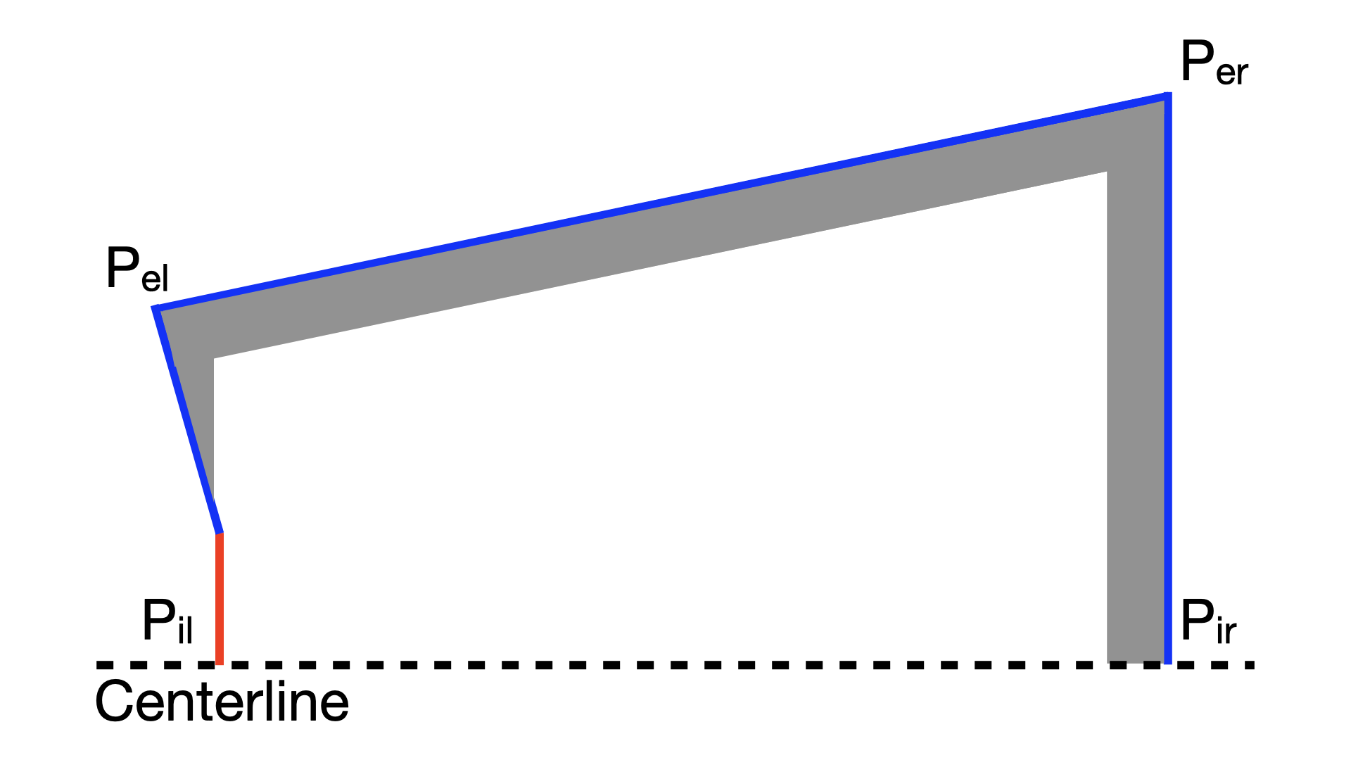
Figure 2: Schematic representation of an axisymmetric plane of the physical domain used for the jet flow simulations.

3.2 Numerical Meshes

The FLEXI solver uses exclusively hexahedral grid elements for computational purposes[30]. Hence, the grid generation led to an integrated process to generate the computational domain and the numerical mesh. The computational domain comprises the three-dimensional version of the control volume illustrated in Fig. 2 with the dimensions provided in Sec. 3.1. The geometries are generated with the open-source mesh generator Gmsh[50].

The mesh generation follows the multi-block strategy, where the computational domain is divided into big blocks of 6-sided volumes. The multi-block mesh generation with Gmsh requires that the block topology is defined in the computational domain. The generation of the G1 geometry and the first block topology follows the reference work[7], with adjustments from the axisymmetric construction of the grid applied in the cited reference to the multi-block strategy employed in the present work. A cut plane through the centerline of the G1 geometry is presented in Fig. 3a with the block distribution. After the simulations performed with the G1 geometry and the meshes originated with the proposed topology, a new multi-block topology was generated utilizing the G2 geometry as the reference domain. A cut plane through the centerline of the G2 geometry is presented in Fig. 3b to show the differences between the topology used in the two geometries. A view of the mesh blocks in a crossflow plane is presented in Fig. 3c.

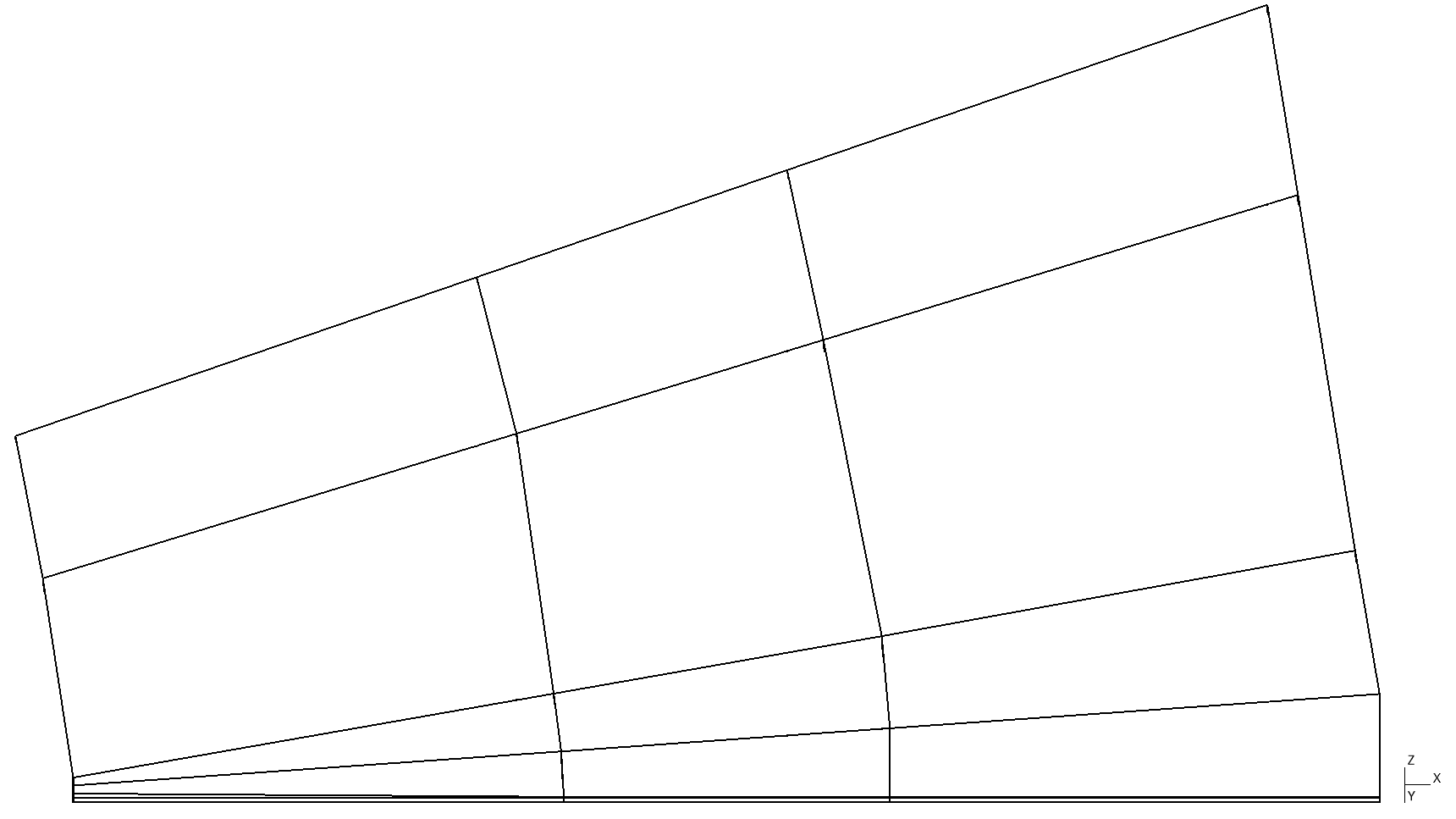
(a) Block topology for G1 geometry.

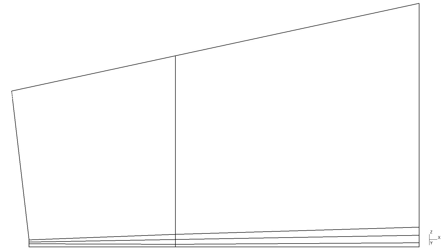
(b) Block topology for G2 geometry.

(c) Block topology in crossflow plane at ${x/D_{j}=0.0}$ for the G2 geometry.

Figure 3: Longitudinal and transversal cut planes presenting the block topologies for the geometries used in the work.

Three numerical meshes are generated to discretize the computational domain. The first two numerical meshes are named M-1 and M-2. They are generated using the G1 geometry, and they have approximately $6\times 10^{6}$ and $1.8\times 10^{6}$ elements, respectively. When performing a simulation with the M-1 mesh and a second-order accurate spatial discretization, the total number of degrees of freedom from the simulation is approximately the same as the simulation of the M-2 mesh with third-order accurate discretization. In summary, the first two numerical grids are designed to investigate the influence of the order of accuracy in the solution of a jet flow with a constant number of degrees of freedom.

The third mesh generated has a different topology and a higher number of elements when compared to the first two meshes. It was generated to enclose a larger refinement in the region of the lipline close to the nozzle exit section and a smooth transition through the domain centerline with increasing distance from the jet inlet section. The local mesh refinement in the jet lipline and the axial mesh refinement are in agreement with other numerical grids from different jet simulations[4, 17, 6, 5]. This numerical mesh, named M-3 mesh was designed to capture the jet within the section of $x/D_{j}=15.0$. After that point, the mesh coarsens at a higher rate to damp oscillations that could introduce instabilities to the simulation. The G2 geometry is employed for the generation of the M-3 mesh. The numerical grid also has higher coarsening rates in radial positions farther from the jet. Based on the results of the simulations using M-1 and M-2 meshes, the jet opening angle evaluated is approximately $2$ degrees.

The radial mesh refinement in longitudinal positions $x/D_{j}=0.0$ and $x/D_{j}=15.0$ are presented in Figs. 4a and 4b, and longitudinal distributions of mesh elements are presented in Fig. 4c. In the azimuthal direction, the M-1 mesh has one element every $2$ degree, the M-2 mesh has one element every $3$ degree and M-3 mesh has the same distribution as the M-1 mesh. The three numerical meshes’ half-domain longitudinal cut planes are presented in Fig. 5. A summary of the information from the numerical geometries and meshes is presented in Tab. 1

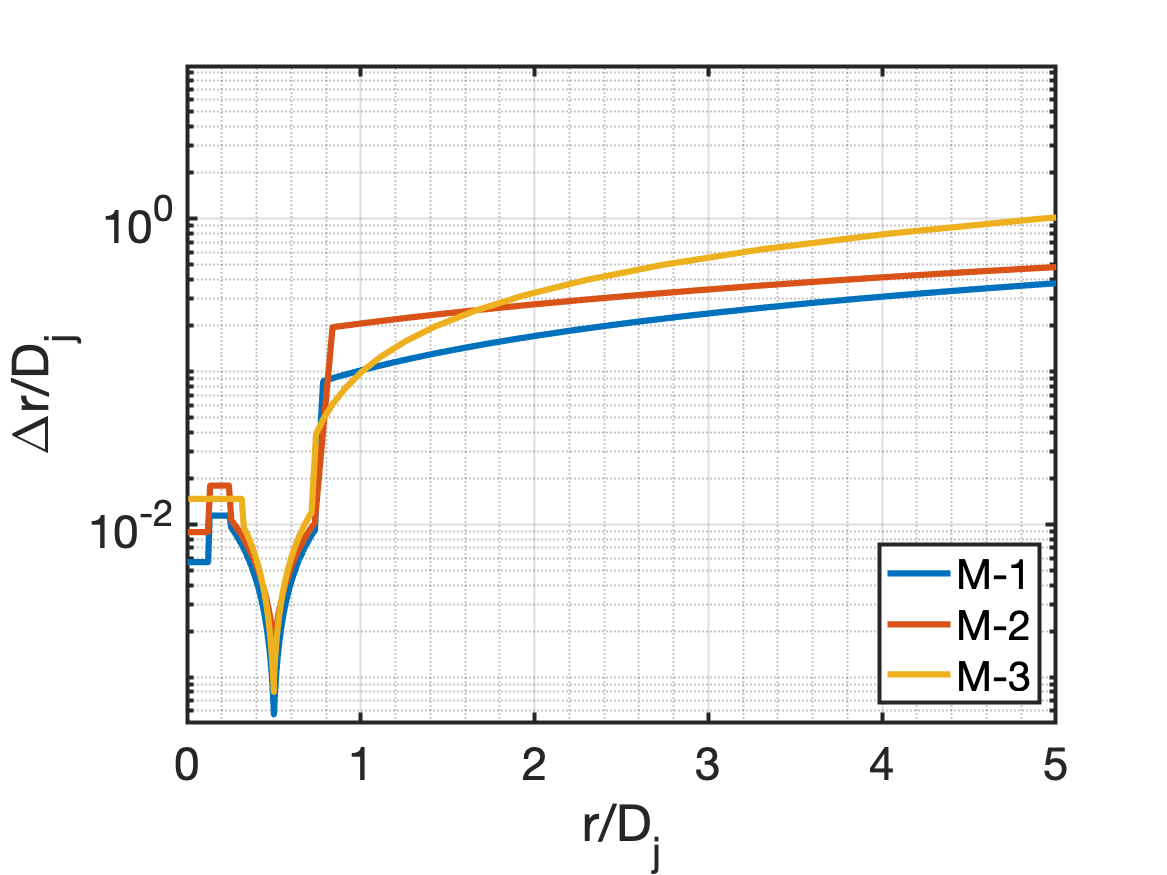
(a) Radial mesh refinement at $x/D_{j}=0$.

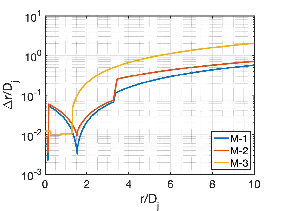
(b) Radial mesh refinement at $x/D_{j}=15.0$.

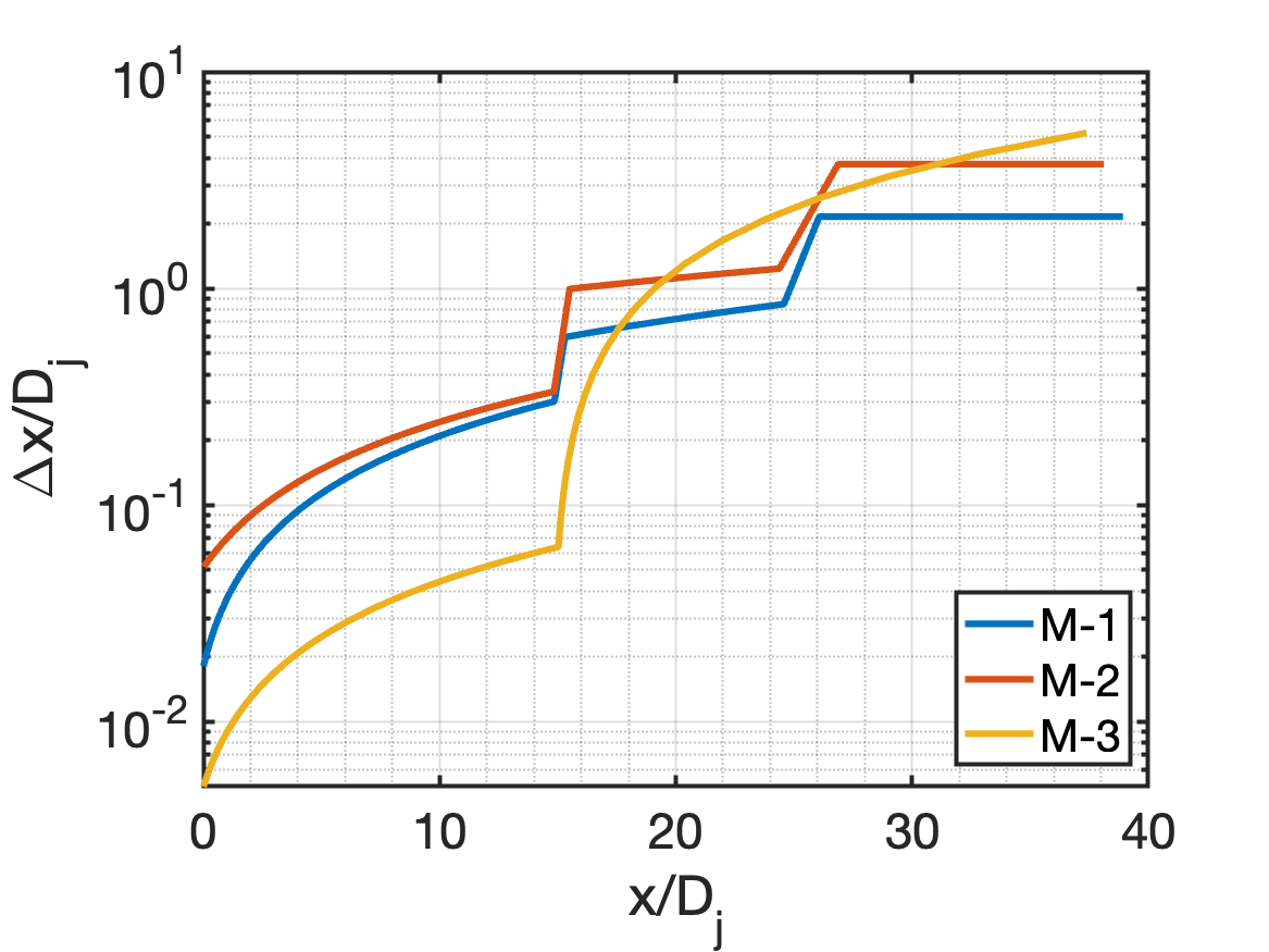
(c) Longitudinal mesh refinement at the jet centerline $r/D_{j}=0.0$.

Figure 4: Distribution of grid spacing indicating radial and longitudinal refinement for the three numerical meshes.

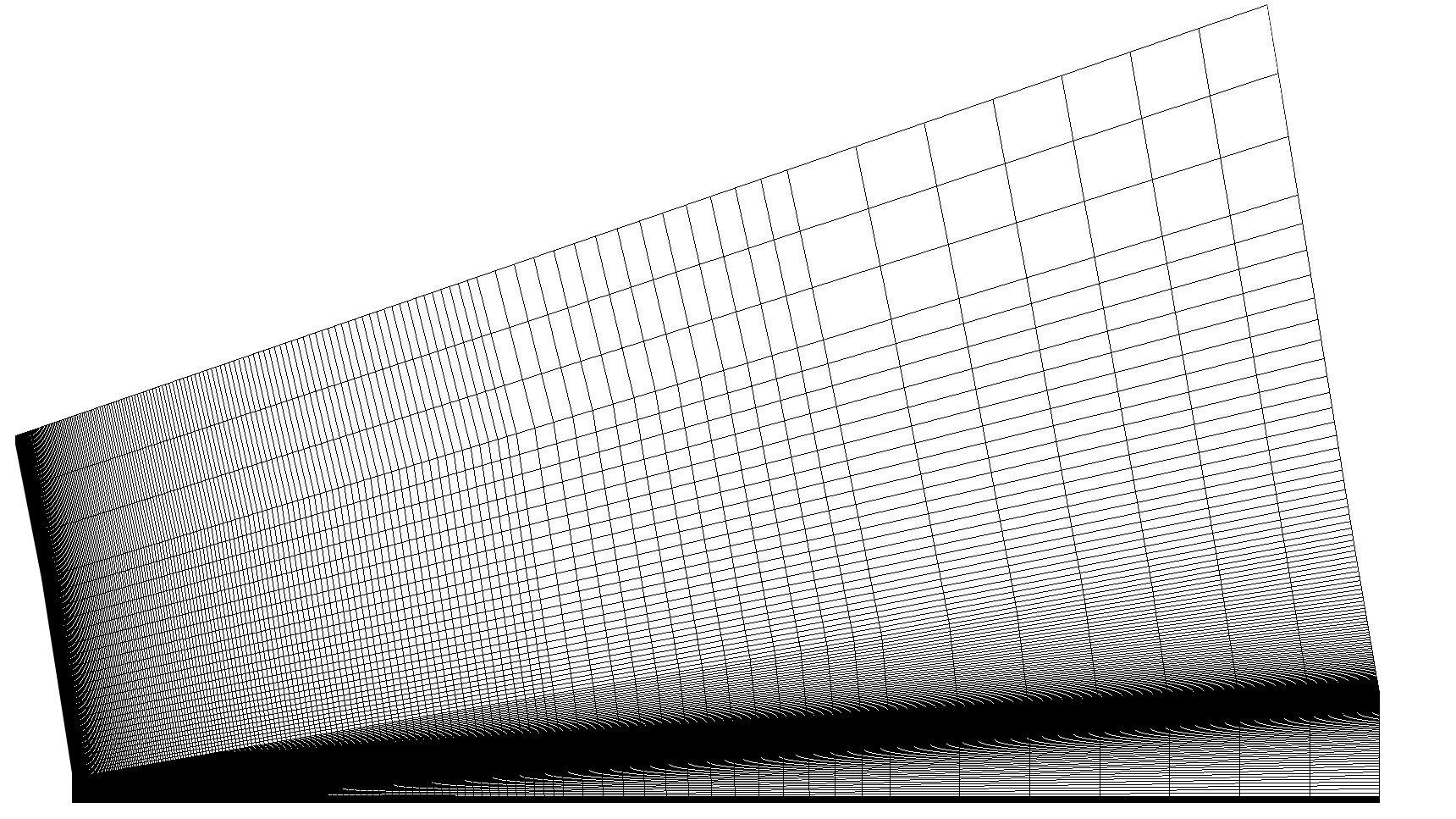
(a) M-1 mesh.

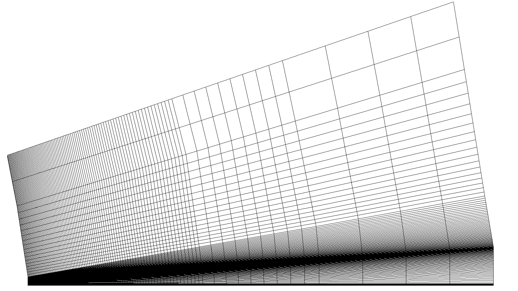
(b) M-2 mesh.

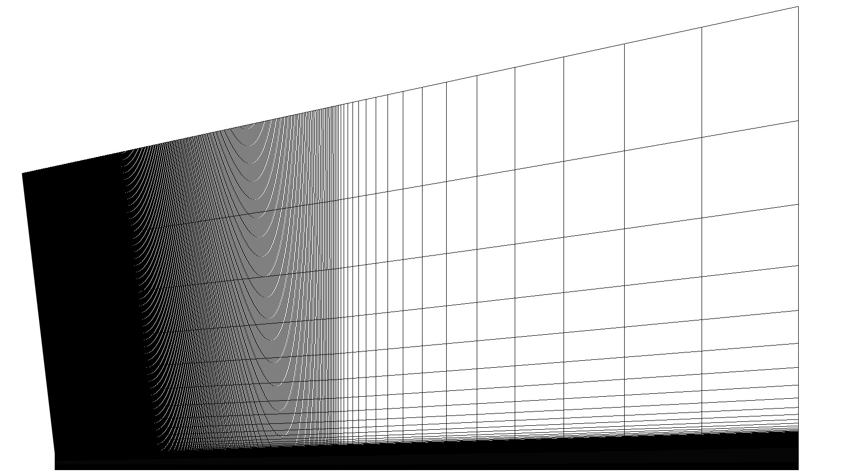
(c) M-3 mesh.

Figure 5: Visualization of the half-domain longitudinal cut planes for the meshes used in the present work.

Table 1: Characteristics of the three numerical meshes used in the work.

Numerical	Computational	Elements	Topology
Meshes	Domain	($10^{6}$)
M-1	G1	$6.2$	Legacy
M-2	G1	$1.8$	Legacy
M-3	G2	$15.4$	Improved

4 Numerical Procedure

The definition of the computational domain and generation of the numerical mesh is the starting point for the performance of the numerical simulations. It is necessary to specify the boundary conditions to be used in the domain’s boundaries. The definition of the polynomial degree to represent the numerical solution influences the order of accuracy of the numerical simulation and the limits of stability of the computational methods. The specification of the boundary conditions, the definition of the simulation settings, and the calculation procedure for the statistical properties are presented in the present section.

4.1 Boundary Conditions

The jet inflow, $(\cdot)_{j}$, and far-field, $(\cdot)_{ff}$, are the two boundary surfaces present in the computational domain. The surfaces are represented by the red and blue lines, respectively, in Fig. 2. The boundary conditions imposed for both surfaces are weakly enforced solutions to Riemann problems in which the flow state outside of the domain is specified. The Riemann solver applied in the boundary condition enforcement is the same one employed to calculate the numerical fluxes between element interfaces. The difference between the boundary conditions rests on the properties of the reference state. An inviscid profile represents the jet inflow condition. The inviscid profile represents a uniform flow with the same properties prescribed independent of radial and azimuthal positions. The properties imposed in the jet inlet condition match the specified Mach number and Reynolds number based on the jet inlet diameter of the experimental reference[2]. The flow is characterized as a perfectly expanded and isothermal, meaning that $p_{j}/p_{ff}=1$ and $T_{j}/T_{ff}=1$, where $p$ stands for pressure and $T$ for temperature. The Mach number of the jet inlet is $M_{j}=1.4$, and the Reynolds number is $Re_{j}=1.58\times 10^{6}$. A small longitudinal velocity component with $M_{ff}=0.01$ is imposed in the far-field boundaries, following the same approach of other jet simulations[22, 6]. A sponge layer model[51] is imposed around the far-field boundary condition, represented by the gray region in Fig. 2, to damp oscillations that could reach the boundary condition and be reflected to the jet flow.

4.2 Simulation Settings

Four simulations assess the influence of “hp” mesh refinements and polynomial degrees on the representation of supersonic jet flows. The simulations utilize the three numerical meshes presented in Tab. 1. Two polynomial degrees are used in the simulations to represent the numerical solution, linear or quadratic polynomials, which yield second and third-order accurate spatial discretization, respectively. In conjunction with the two interpolating polynomial degrees, the ensemble of numerical meshes produced simulations with a total number of degrees of freedom varying from $50\times 10^{6}$ to $410\times 10^{6}$ DOFs. The numerical simulations are named S-1 to S-4 simulations. The simulation ordering is associated with the increasing resolution of the numerical simulations.

The four simulations utilize the same time marching method, a third-order accurate standard Runge-Kutta scheme with three stages. The time step applied to the simulations has a fixed value based on a fraction of the limit of stability for the Courant–Friedrichs–Lewy (CFL) number for the Runge-Kutta method. The CFL number stability limit varies with the polynomial degree used to represent the numerical solutions. High polynomial degrees present larger restrictions on the maximum CFL than small ones. The numerical simulations are performed with a fraction of the maximum CFL of $0.71$, $0.46$, $0.39$, and $0.49$ from the S-1 to S-4 simulations. The S-3 simulation is performed with a conservative time step, while the other three are advanced in time with an overall CFL number closer to the corresponding stability limits. Table 2 indicates the settings used in the four numerical calculations.

Table 2: Summary of simulations settings.

Simulation	Numerical	Polynomial	Order of	Degrees of
		Degree	Accuracy	Freedom ($10^{6}$)
S-1	M-1	Linear	2nd order	$\approx 50$
S-2	M-2	Quadratic	3rd order	$\approx 50$
S-3	M-3	Linear	2nd order	$\approx 120$
S-4	M-3	Quadratic	3rd order	$\approx 410$

The development of the numerical simulations involved two steps. The jet flow solution is let to develop from its initial condition to a statistically steady flow. Then, the data acquisition is performed. The initial condition of the simulation is a quiescent flow for simulations S-1 to S-3. The S-4 simulation used the solution from the S-3 simulation as the initial condition, which reduced the simulation time to reach the statistically steady condition. A non-dimensional time scale is employed as a reference for the evolution of the simulation. The non-dimensional time, which is called flow-through time (FTT), is defined with the jet inlet velocity ($U_{j}$) and the jet inlet diameter ($D_{j}$). It was observed that starting the simulation with a quiescent flow required approximately $240$ FTT to reach a statistically steady flow, and using a previous solution reduced the development time to approximately $100$ FTT.

The simulations were conducted at the Jean-Zay supercomputer from the IDRIS computing center [52]. A total of $800$ to $1300$ CPUs were used to perform the simulations, depending of the test case addressed. The computational cost of the simulations was approximately $100\times 10^{3}$ CPU hours for the S-1 and S-2 simulations and $300\times 10^{3}$ for the S-3 simulation. The computational cost of the S-4 simulation was reduced due to the restart from the solution of the S-3 simulation. After the restart, the computational cost to conclude the S-4 simulation was approximately $500\times 10^{3}$ CPU hours.

4.3 Calculation of Statistical Properties

The acquisition time is in agreement with the smallest Strouhal number ($St$) used in the experimental reference[2] and from other numerical work that evaluated a similar jet flow condition[22]. The acquisition frequency is determined to provide a high value of the maximum Strouhal number to be investigated. The acquisition frequency used is $200$ kHz. Estimating the maximum Strouhal number through $St_{max}=fD_{j}/2U_{j}$ and the minimum Strouhal number by $St_{min}=D_{j}/t_{s}U_{j}$, where $f$ is the acquisition frequency and $t_{s}$ is the time sample, the values of $St_{max}=10.5$ and $St_{min}=0.01$ are obtained.

Flow properties’ mean and root mean square (RMS) fluctuations are calculated along the longitudinal distributions at the centerline and lipline and radial distributions at four streamwise positions. The centerline is defined as the line in the center of the geometry $r/D_{j}=0.0$, whereas the lipline is a cylindrical surface at the nozzle diameter, $r/D_{j}=0.5$. The four streamwise planes are at $x/D_{j}=2.5$, $x/D_{j}=5.0$, $x/D_{j}=10.0$, and $x/D_{j}=15.0$. Spectral analysis is conducted. The Power Spectral Density (PSD) of the longitudinal and radial velocity fluctuations are performed at the lipline in the four streamwise planes.

5 Flow Field Result Analyses

The results of the four simulations are compared to assess the “hp” mesh refinement and polynomial degree improvements obtained with the increase in the simulation resolution. Due to axisymmetry of the jet flow the results are presented in the polar coordinate system $\boldsymbol{U}=(U_{x},U_{r},U_{\theta})$. A qualitative analysis is performed with contours of instantaneous and statistical properties. A quantitative analysis is performed with the longitudinal and radial distributions at the centerline, lipline, and the four streamwise planes. In the quantitative analysis, the results of the four simulations are compared with experimental data. A signal analysis is performed with the power spectral density of the velocity fluctuation in the lipline.

5.1 Instantaneous Flow Field

The instantaneous contours of velocity and pressure from the jet flow field are investigated in order to visualize the flow features presented by the numerical simulations. The instantaneous longitudinal velocity component contours presented in Fig. 6 show that in the mixing layer from the S-3, Fig. 6c, and S-4, Fig. 6d, simulations present smaller eddies than those in the mixing layer from the of the S-1, Fig. 6a, and S-2, Fig. 6b, simulations. The velocity contours in the lipline of the jet flow indicate a transition occurring closer to the jet inlet section for the S-3 and S-4 simulations than in the S-1 and S-2 simulations. In the S-1 and S-2 simulations, the interaction of the shock waves is weak, producing few changes to the velocity distribution in the interior of the jet flow. The higher resolution from S-3 and S-4 simulations than the S-1 and S-2 simulations reproduce more intense shock interactions, which affects the flow in the interior of the jet flow, which can be visualized by the many velocity changes in the interior of the jet flow.

The vorticity contours, presented in Fig. 7 highlight the instabilities responsible for the transition from laminar to turbulent and the interaction between the shock waves and the mixing layer. The pressure contours highlight the interaction between the shock waves in the interior of the jet flow and the pressure wave propagation external to the jet flow. The vorticity calculated by the S-1 simulation, Fig. 7a indicate the presence of weak vortices close to the jet inlet section that almost dissipate when it advances in the domain. The increase in the order of accuracy from S-1 to S-2 simulation, Fig. 7b, can produce better-defined vortices capable of sustaining the presence of turbulent eddies with the advance in the domain. In the S-1 and S-2 simulations, the pressure contours indicate the presence of large-scale pressure waves associated with the vortical structures reproduced in the mixing layer. The simulations that used the M-3 mesh, the S-3 and S-4 simulations, could represent additional features in the pressure and vorticity contours. The vorticity contours from the S-3 simulation, Fig. 7c, shows that the simulation can reproduce small-scale vortices responsible for the transition of the flow, and more shock waves are present, which produce a series of pressure changes in the interior of the jet flow. The S-4 simulation, Fig. 7d, presents the best-defined eddies in the mixing layer and shock waves in the interior of the jet flow from the four simulations analyzed. The comparison among the pressure contours and vorticity magnitude contours from the four simulations show a reduction of the numerical dissipation, with the capability of the high-resolved simulations to maintain the flow features correctly represented for longer distances and, also, to include the representation of smaller features present in the flowfield.

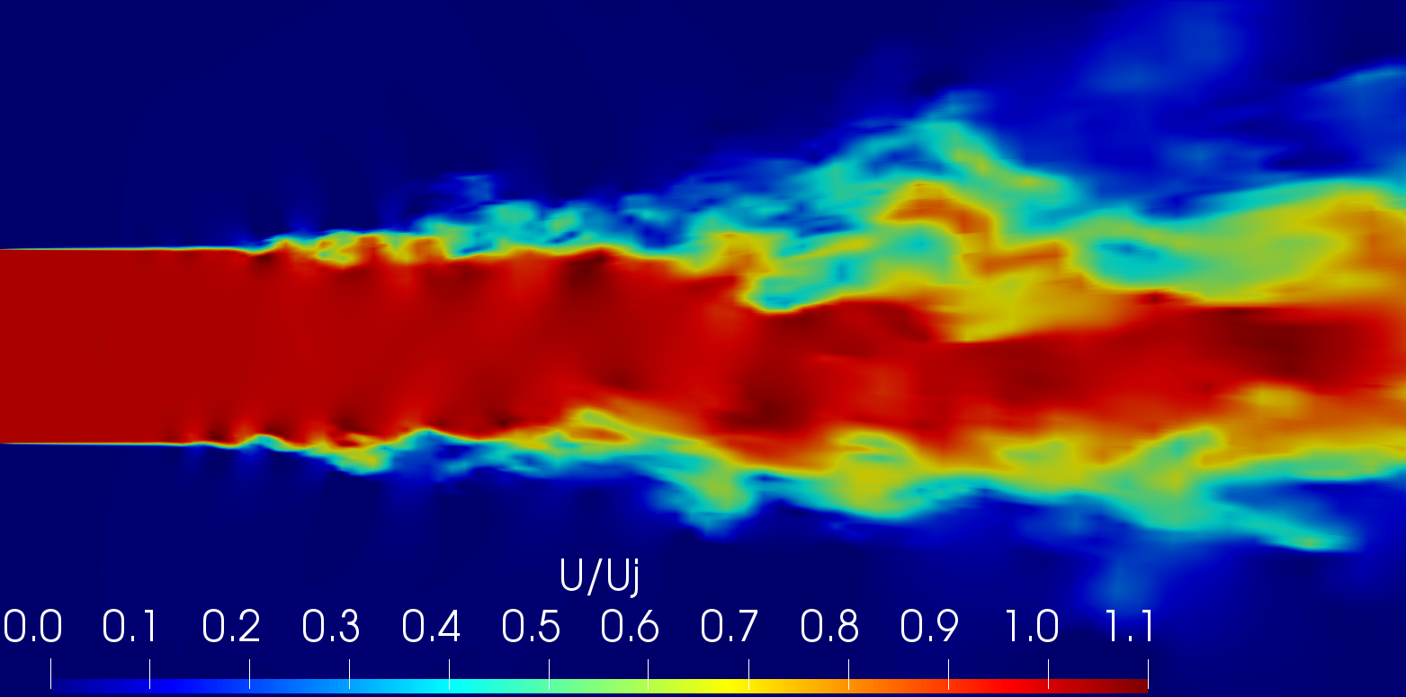
(a) S-1 simulation.

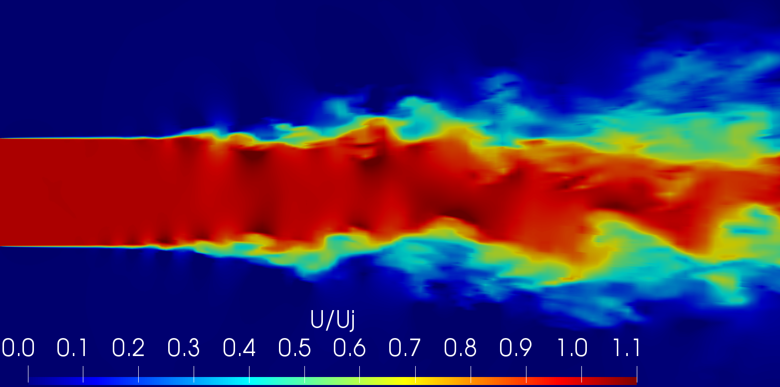
(b) S-2 simulation.

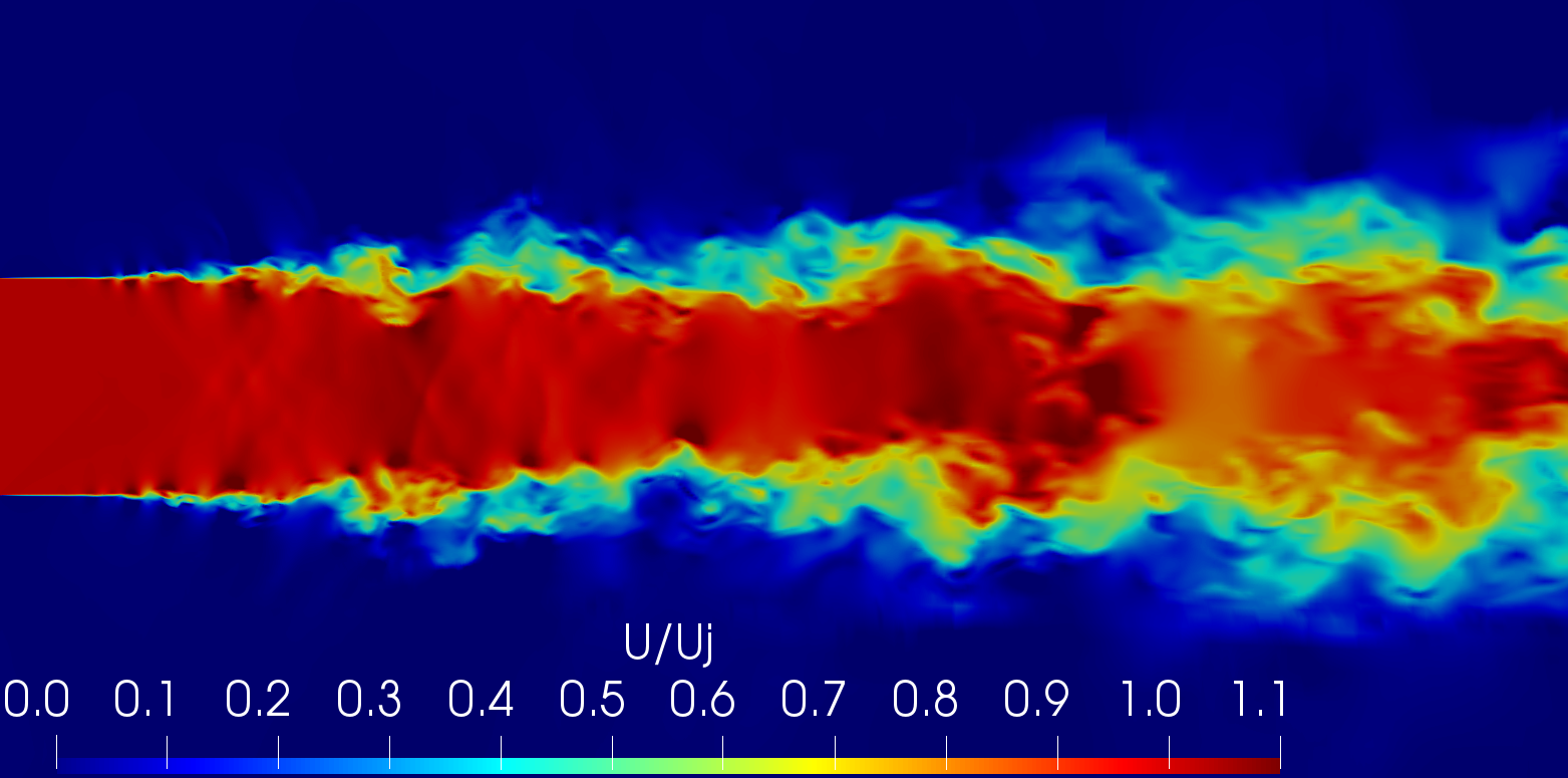
(c) S-3 simulation.

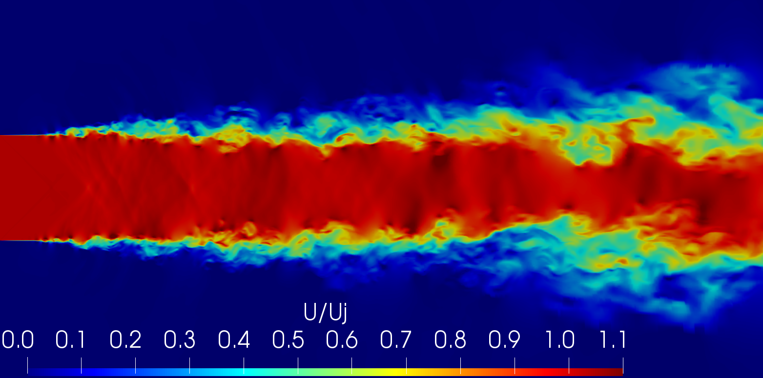
(d) S-4 simulation.

Figure 6: Instantaneous longitudinal velocity component contours on a plane through the centerline of the jet.

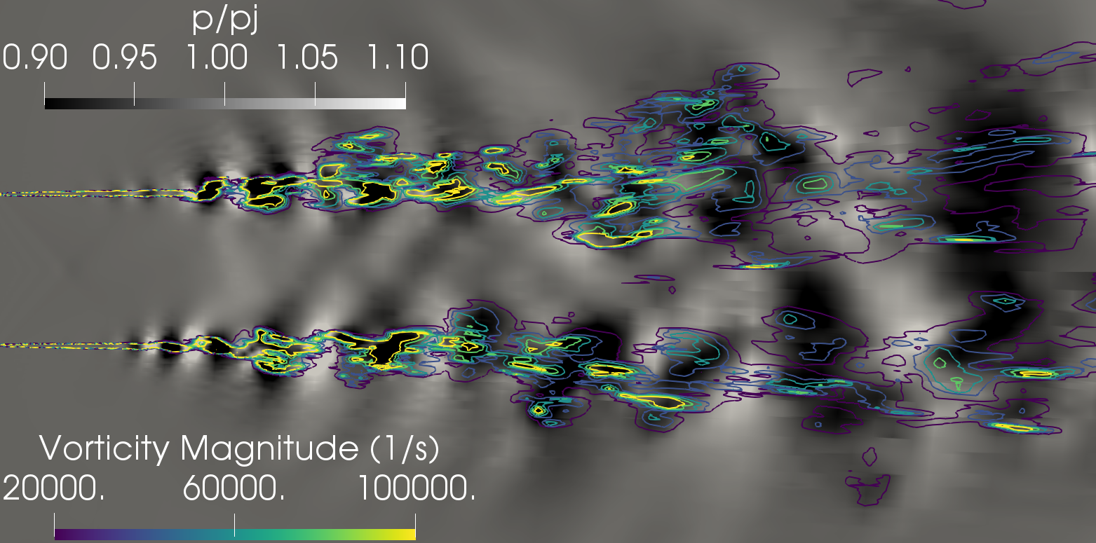
(a) S-1 simulation.

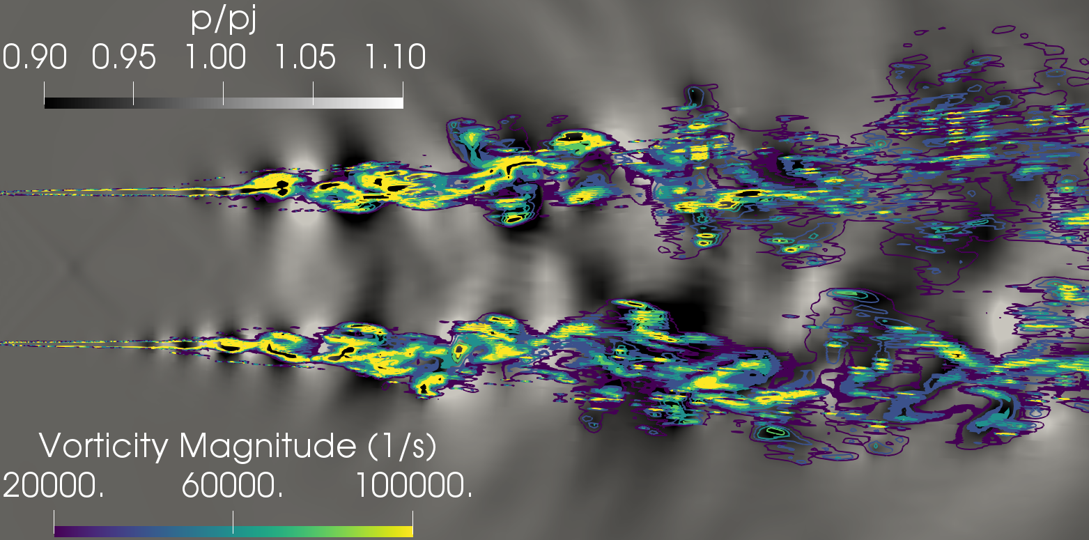
(b) S-2 simulation.

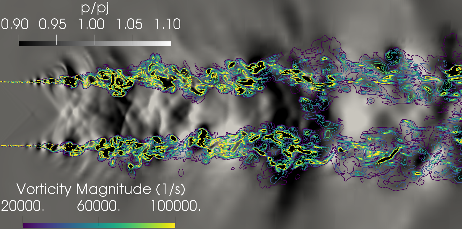
(c) S-3 simulation.

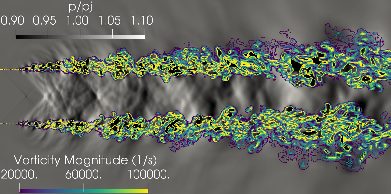
(d) S-4 simulation.

Figure 7: Snapshots of pressure with superimposed contours of vorticity magnitude on a plane through the centerline of the jet flow.

5.2 Mean Flow Field

The contours of the mean longitudinal velocity component, presented in Fig. 8, provide some qualitative information on the distinct calculations of the potential core from each simulation. The jet potential core is the region of the jet with a longitudinal velocity higher than $0.95U_{j}$, where $U_{j}$ is the jet inlet velocity. The length of the potential core is the distance in the centerline of the jet from the inlet section to the position where the velocity reaches the boundary of the potential core, $U=0.95U_{j}$. Comparing the velocity contours in Fig. 8a and Fig. 8b, from S-1 and S-2 simulations, one can observe that the S-2 simulation presents a slightly longer core. Both simulations present a subtle velocity change associated with the shock waves. The velocity contours from the simulations performed with the more refined mesh, Figs. 8c and 8d, present longer jet cores, larger shock waves, and the mixing layer development commences closer to the jet inlet condition than the contours from the S-1 and S-2 simulations. The comparison of the velocity contours from simulations S-3 and S-4 shows a longer potential core with a narrow mixing layer when increasing the resolution from the S-3 to S-4 simulations.

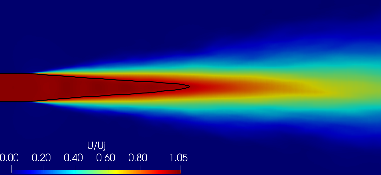
(a) S-1 simulation.

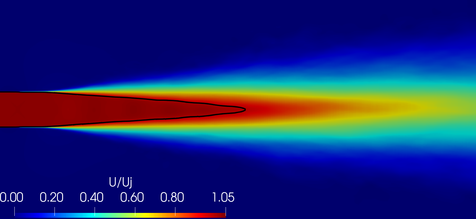
(b) S-2 simulation.

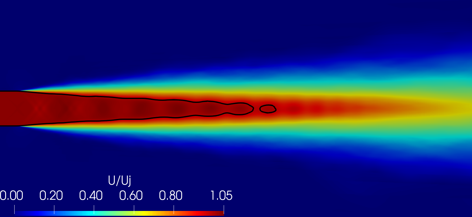
(c) S-3 simulation.

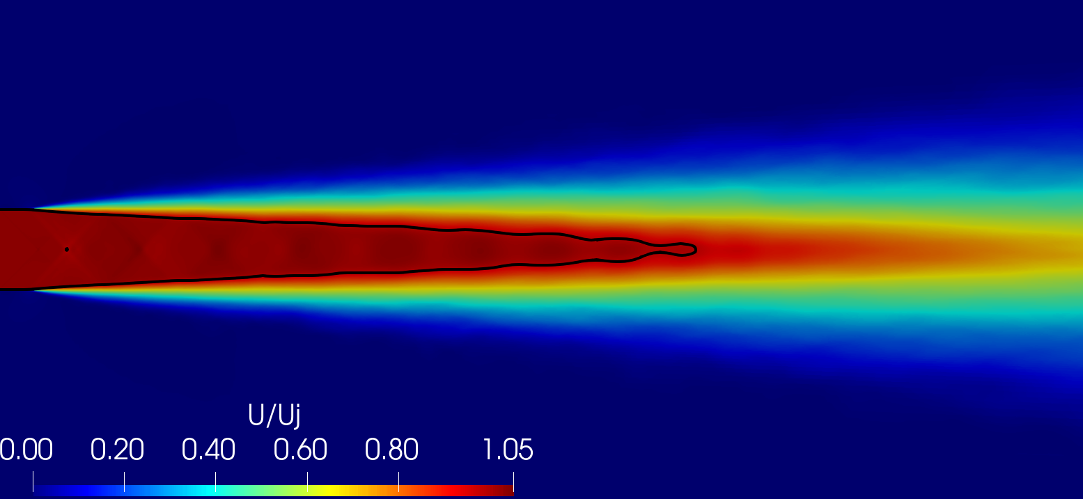
(d) S-4 simulation.

Figure 8: Contours of mean non-dimensional longitudinal velocity component for the simulations performed. The black contour indicate the boundaries of the jet potential core, $U=0.95U_{j}$.

A deeper investigation of the mixing layer can be performed by visualizing the contours of the root mean square (RMS) of the longitudinal velocity fluctuation, presented in Fig. 9. Due to the interaction between the jet flow and the ambient air, the turbulence levels in the mixing layer are higher than in other parts of the flow, and the longitudinal velocity fluctuation presents information on the turbulence levels. In the contours presented in Figs. 9a and 9b, from the S-1 and S-2 simulations, the values of the peak of RMS of the longitudinal velocity component and the spreading of velocity fluctuation in the longitudinal and transversal directions are similar. The velocity contours from the S-3 and S-4 simulations, Figs. 9c and 9d, show some differences in the mixing layer development. The commencement of the development of the shear layer and the peak values occurs close to the inlet section. The contours present minor transversal spreading of velocity fluctuation, which can be observed by the more extended region unaffected by the mixing layer in the centerline and the narrow region with high fluctuation.

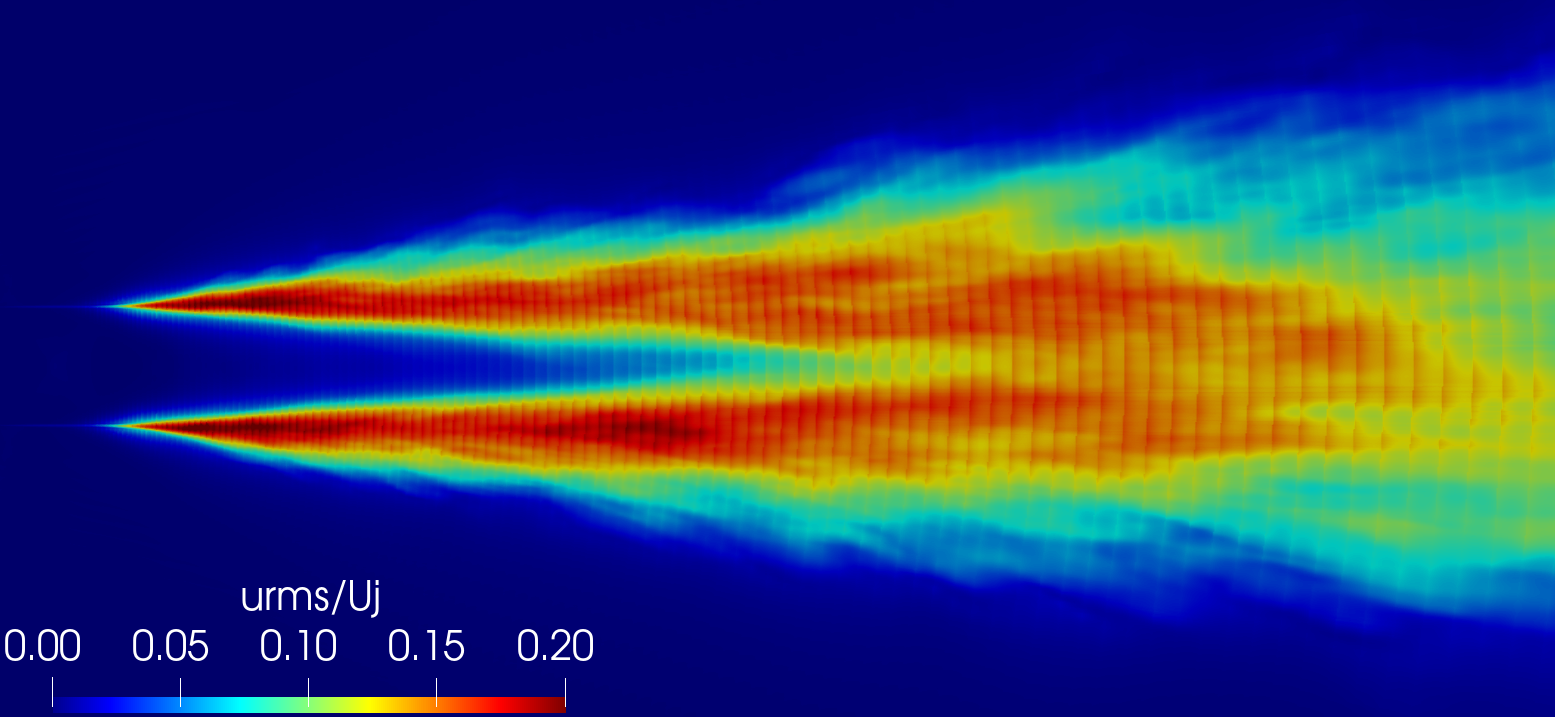
(a) S-1 simulation.

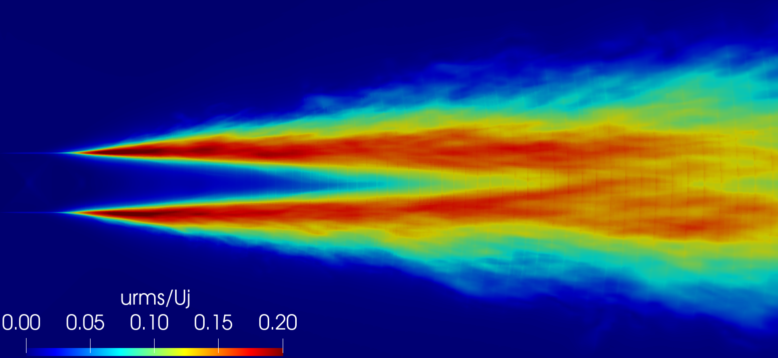
(b) S-2 simulation.

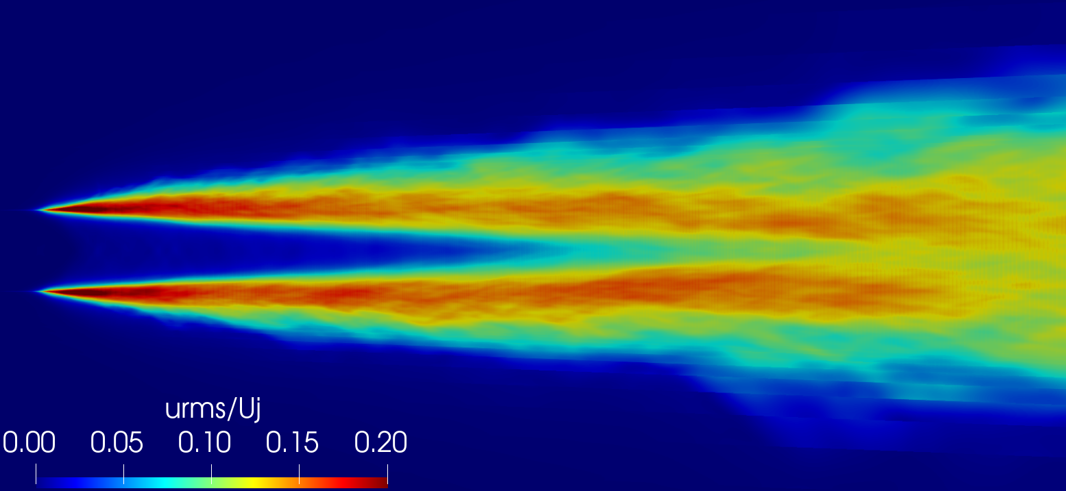
(c) S-3 simulation.

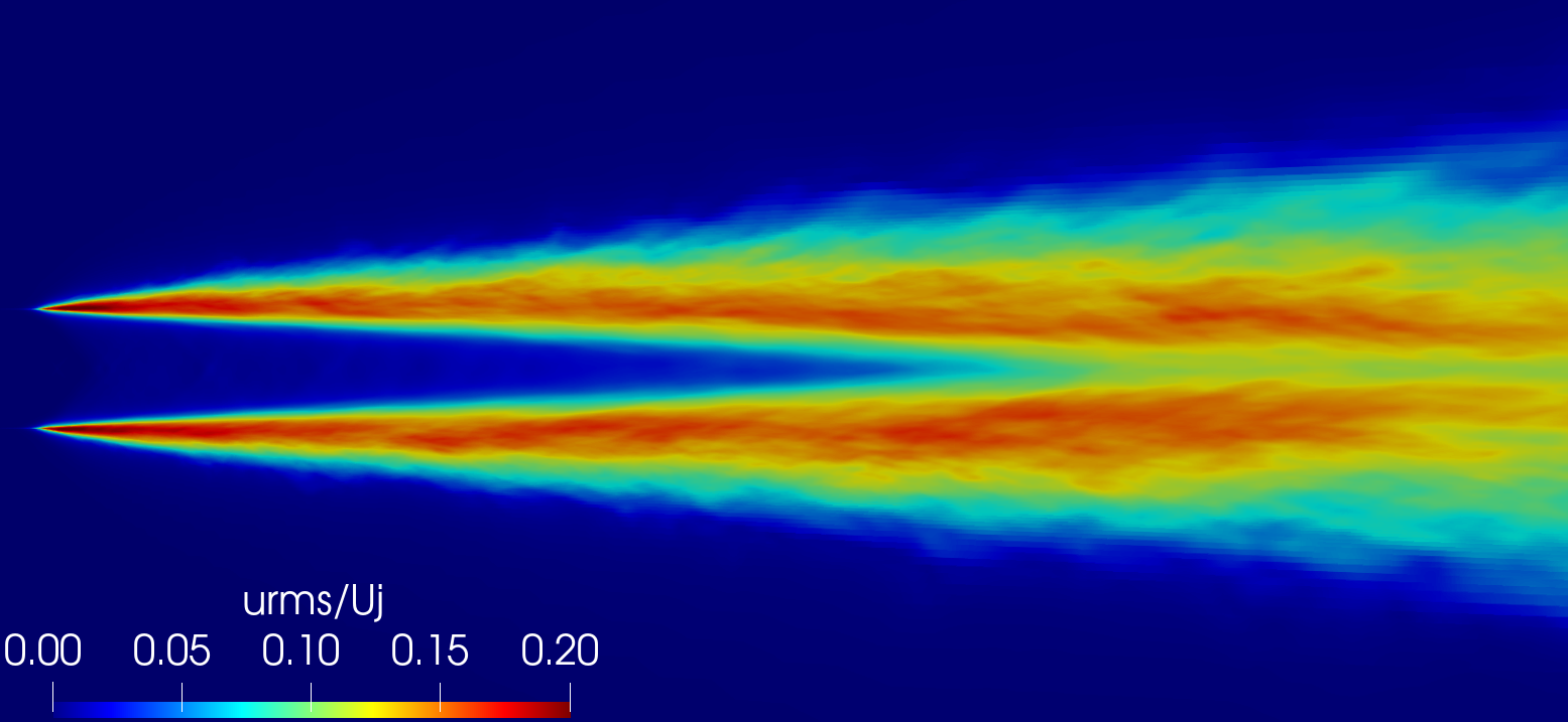
(d) S-4 simulation.

Figure 9: Contours of root mean square non-dimensional longitudinal velocity component fluctuations.

The contours of mean pressure highlight the differences in the simulations concerning the shock wave formation present in the jet core, Fig. 10. The contours from the S-1 simulation, Fig. 10a, indicate a non-uniform pressure distribution, which is associated with the lack of hp-resolution of the simulation in conjunction with the interpolation of the simulation data to the set of probes used for the statistical analyses. The pressure contours from the S-2 simulation, Fig. 10b, presents a smoother transition when compared to the contours from the S-1 simulation, and additional shock waves are present. Significant differences appear when comparing the pressure contours from the S-3 and S-4 simulations, Figs. 10c and 10d, with the contours from the S-1 and S-2 simulations, The shock waves present a larger number of repetitions distributed over a larger region than the reproduced by the S-1 and S-2 simulations. The first shock wave is closer to the inlet section in the S-3 simulation than the S-2 simulation contours. The first shock waves from the S-3 and S-4 simulations present a smaller thickness when compared to the pressure contours from the S-1 and S-2 simulations. The better-defined shock waves are associated with a better resolution from the S-3 and S-4 simulations when compared to the S-1 and S-2 simulations. The pressure contours from the S-4 simulation indicate thin shock waves compared to the S-3 simulation. However, the shock waves from the S-3 simulation present larger pressure differences between the repetitions than those of the S-4 simulation.

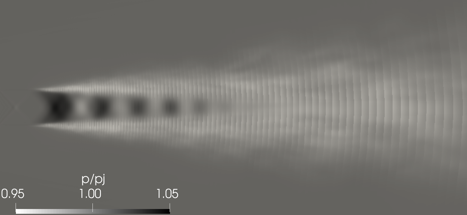
(a) S-1 simulation.

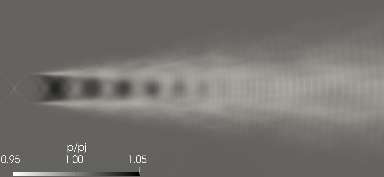
(b) S-2 simulation.

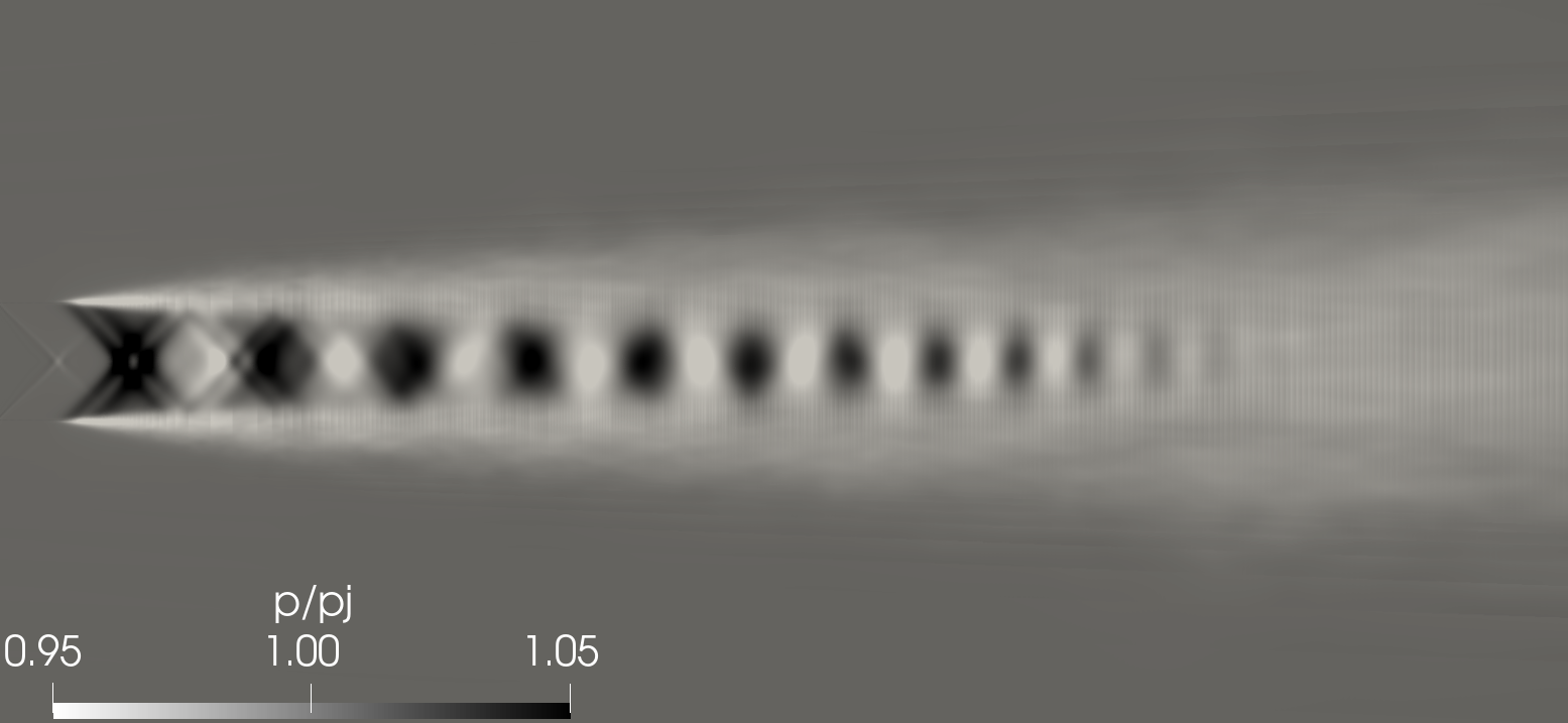
(c) S-3 simulation.

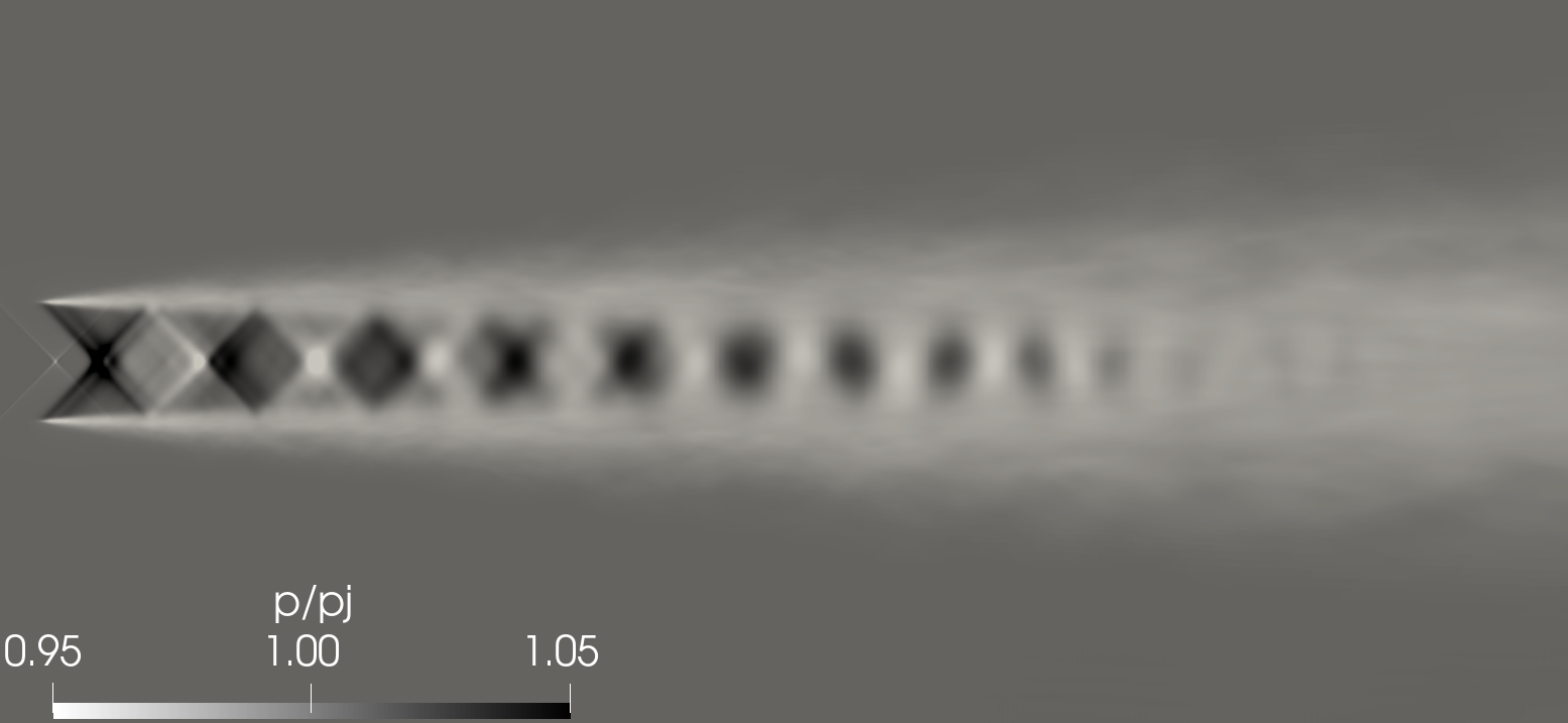
(d) S-4 simulation.

Figure 10: Mean non-dimensional pressure contours from the simulations performed.

5.3 Longitudinal Profiles of Velocity and Reynolds Stress Tensor

The velocity distribution of the four simulations is quantitatively compared with experimental data[2] at the centerline and lipline, Fig. 11. Figures 11a and 11b present the mean longitudinal velocity component distribution and the RMS of the longitudinal velocity fluctuation distribution at the centerline of the jet flow. The mean longitudinal velocity component distribution presents a general behavior between the simulations. Close to the jet inlet section, inside the potential core of the jet flow, the velocity values are only affected by the shock waves. Close to the potential core length, the velocity distribution presents a negative slope associated with the mixing layer of the jet flow spreading the velocity from the jet core. The S-1 and S-2 simulations present a shorter potential core length when compared to the S-3 and S-4 simulations. The short potential core length, which is close to the change of the velocity slope, occurs close to $x/D_{j}=7.0$. The change in the slope from the experimental data is only observed downstream of the jet flow. The velocity distribution from the S-2 simulation indicates a slightly longer potential core when compared with the S-1 simulation. The velocity distribution from the S-3 and S-4 simulations are closer to the experimental reference when compared to the S-1 and S-2 simulations. The potential core length is close to $x/D_{j}=8.0$, and there is a visible influence of the set of shock waves through the jagged distribution in the potential core. In the S-1 and S-2 simulations, a series of shock waves with small velocity peak to peak velocity amplitude can be observed up to the section $x/D_{j}\approx 6$, while in the S-3 simulation the set of shock waves extend up to $x/D_{j}\approx 10$. The S-4 simulation presents a better agreement with experimental data when compared to the other simulations. The potential core from the S-4 simulation is longer than the potential core from the S-3 simulation. The peak-to-peak velocity amplitude in the potential core from the S-4 simulation is minor than the S-3 simulation. The potential core length is used as a parameter to assess the error of the numerical simulations. The results of the error assessment are presented in Tab. 3.

The RMS of the longitudinal velocity fluctuation distribution in the centerline, Fig. 11b, indicates an improvement from the simulation results with increased resolution compared to the experimental reference. The longitudinal velocity fluctuation distributions from the S-1 and S-2 simulations present an increase in the velocity slope occurring closer to the jet inlet section than the S-3 and S-4 simulations and the experimental data. The velocity fluctuation distribution from the S-1 simulation presents oscillation in the velocity distribution that may be associated with employing a relatively coarse mesh and linear polynomial degree with the probe processing employed to interpolate data in the flow field. The results with large mesh refinement or third-order accurate scheme does not present a similar oscillation. The velocity fluctuation of the S-3 simulation presents a reduced maximum RMS value when compared to the maximum values from the S-1 and S-2 simulations. The reduced maximum values from the velocity fluctuation distribution and the change in the velocity slope occurring far from the inlet section led the velocity fluctuation distribution to approach the experimental reference. In the present property evaluated, the S-4 simulation provided results that better match the experimental reference than the other numerical simulations.

Figures 11c and 11d present the distribution of the mean longitudinal velocity component and the RMS of the longitudinal velocity fluctuation at the lipline of the jet flow. The mean longitudinal velocity component distribution at the lipline, Fig. 11c, indicate that in the region $0<x/D_{j}<5.0$ the four simulations and the experimental data present similar values. The velocity distributions from the S-1 and S-2 simulations present a change in the velocity slope, which resulted in smaller mean velocity velocities. The change in the velocity slope occurs after the position $x/D_{j}\approx 5.0$ for the S-1 simulation and for $x/D_{j}\approx 7.0$ for the S-2 simulations. The mean velocity distributions from the S-3 and S-4 simulations indicate similar velocity values along the longitudinal region evaluated.

The distributions presented for the RMS of the longitudinal velocity fluctuation at the lipline, Fig. 11d, have a different behavior than the previous analyses from Figs. 11a, 11b, and 11c. The four simulations present an abrupt change in the slope of the velocity fluctuation distribution in the region $0.0<x/D_{j}<2.0$. After the abrupt increase in the velocity fluctuation levels, the distributions reach maximum velocity fluctuation values significantly larger than those from the experimental reference. After reaching the maximum value, an inversion in the velocity distribution slope is observed. The velocity slope inversion led to the S-1, S-2 and S-3 simulations to present velocity fluctuation levels above the experimental reference for $x/D_{j}>12.0$. The S-3 and S-4 simulations present a similar behavior of velocity fluctuation in the lipline. In these two simulations, the abrupt change in the velocity slope occurs in a station even closer to the jet inlet section, $x/D_{j}\approx 0.5$, when compared to the change in the slope from the S-1 and S-2 simulations, $x/D_{j}\approx 1.0$, and reaches its peak close to $x/D_{j}=1.0$. The velocity fluctuation distribution from the S-4 simulation never reaches velocity values below those of experimental data. The velocity fluctuation distribution shows that the growth in the velocity fluctuation occurs closer to the jet inlet section with increased resolution, except for the S-1 and S-2 simulations. Even though the S-1 simulation is simulated with a second-order accurate spatial discretization, it has a more refined mesh than the S-2 simulation, which may be responsible for allowing the simulation to capture smaller eddies than those of the S-2 simulation. Once the same mesh is employed with different spatial discretization accuracy, the third-order accurate method could better reproduce the turbulent eddies than the second-order accurate, allowing the simulation to anticipate the transition mechanism. The results from the velocity fluctuation in the lipline indicates important differences to the experimental data, which are associated with the inviscid profile imposed in the jet inlet section and not related to a lack of accuracy of the numerical method.

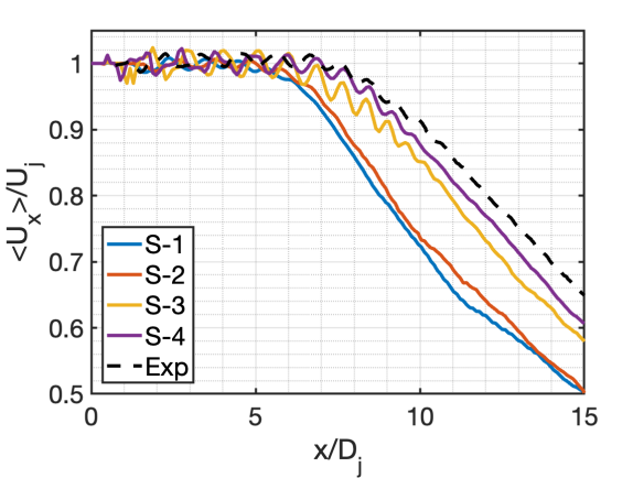
(a) Mean velocity distribution at the centerline.

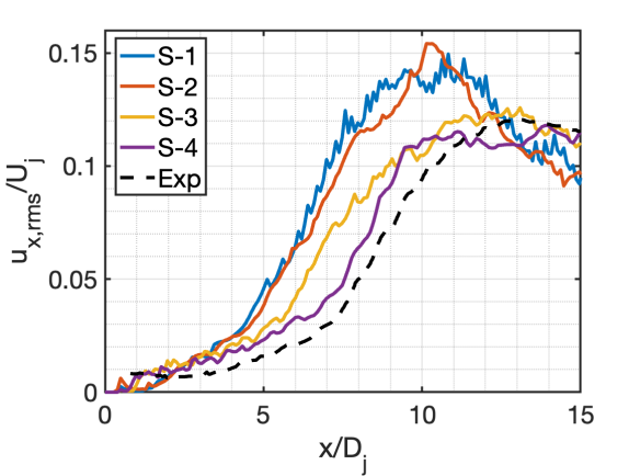
(b) RMS of velocity fluctuation distribution at the centerline.

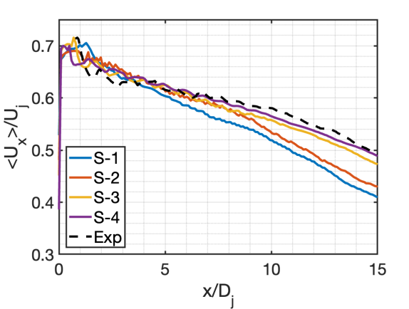
(c) Mean velocity distribution at the lipline.

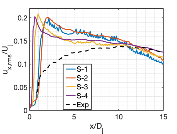
(d) RMS of velocity fluctuation distribution at the lipline.

Figure 11: Longitudinal distributions of the mean longitudinal velocity component and the rms of the longitudinal velocity fluctuation at the jet centerline, $r/D_{j}=0.0$, and lipline, $r/D_{j}=0.5$.

Table 3: Summary of potential core length information for the four numerical simulations performed.

Simulation	Potential core	Error to
	length ($x/D_{j}$)	experimental data ($\%$)
S-1	6.6	25.0
S-2	6.9	21.6
S-3	7.7	12.5
S-4	8.5	3.4

Figure 12 presents the Reynolds stress tensor components at the centerline and lipline of the jet flow. Differently from the previously presented profiles, in Fig. 12 each chart presents the numerical results from one simulation. In Figs. 12a, 12c, 12e, and 12g the Reynolds stress tensor components from the S-1 to S-4 simulations at the jet centerline are presented, and Figs. 12b, 12d, 12f, and 12h present the Reynolds stress tensor components from the S-1 to S-4 simulations at the jet lipline. The longitudinal velocity fluctuation profiles are the same as presented in Figs. 11b and 11d squared, and they are left to reappear in the charts presented in Fig. 12 to simplify the comparison. The Reynolds stress tensor components distribution from the S-1 simulations present the same oscillations observed in Fig. 11b and Fig. 11d, which may be associated probe processing used in the data extraction from the numerical simulations. In the Reynolds stress tensor components distributions at the jet centerline from the S-1 and S-2 simulations, the increase in the three velocity fluctuations occurs closer to the jet inlet section than observed in the experimental reference. The values of the longitudinal fluctuation component present a larger increase than the other components, which, after the maximum values, present an inversion in the Reynolds stress tensor slope until reach values closer to the radial and azimuthal components at $x/D_{j}=15.0$. The Reynolds stress tensor components distribution from the S-3 and S-4 simulations present a better agreement with experimental data than the distributions from the S-1 and S-2 simulations. The increase in the values of the Reynolds stress tensor components occur farther from the inlet section than in the S-1 and S-2 simulations. It can be observed that, except for the longitudinal velocity fluctuation component the from S-1 and S-2 simulations close to station $x/D_{j}=15.0$, the components of the Reynolds stress tensor agrees with experimental data.

The profiles of Reynolds stress tensor components at the lipline indicate that its peak occurs in a station closer to the jet inlet section for the S-3 and S-4 simulations than the S-1 and S-2 simulations due to the higher mesh refinement. The higher mesh refinement allows the S-3 and S-4 simulations to capture small eddies and anticipate the flow transition. The shear-stress tensor component distribution from the S-1 and S-2 simulations present a similar level of the radial component, while the S-3 and S-4 simulations present different velocity levels between all the components. The comparison with experimental data indicates that close to the inlet section, the shear-stress and radial components should present similar results that split with the progress in the flow field. The simulations did not capture the behavior. The S-4 calculation is the one that could get closer to the experimental data when compared to the other calculations. However, it is of most importance to mention that the inlet velocity profile is imposed as an inviscid one, which plays an essential role in the turbulent transition and, consequently, also in the Reynolds stress tensor components. One should notice that the article’s goal is to study the effects of resolution on the calculation, and a boundary condition comparison is out of the scope of the current study.

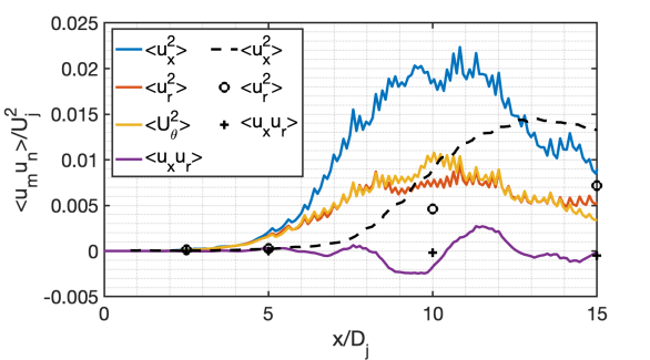
(a) S1 simulation along the centerline.

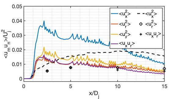
(b) S1 simulation along the lipline.

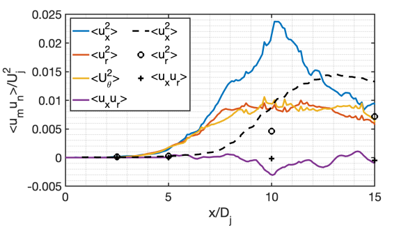
(c) S2 simulation along the centerline.

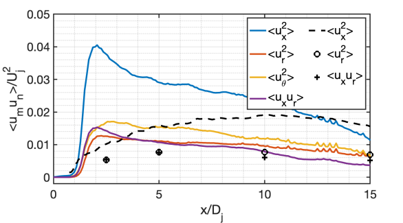
(d) S2 simulation along the lipline.

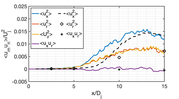
(e) S3 simulation along the centerline.

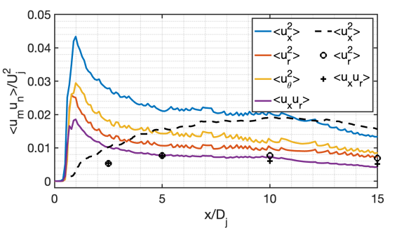
(f) S3 simulation along the lipline.

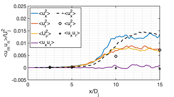
(g) S4 simulation along the centerline.

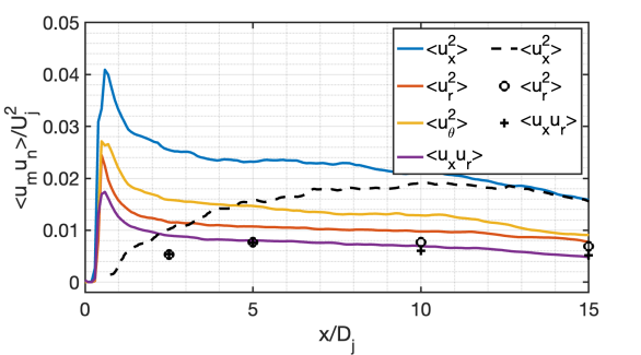
(h) S4 simulation along the lipline.

Figure 12: Reynolds stress tensor components longitudinal distributions from the four simulations analyzed at the jet centerline, $r/D_{j}=0.0$, and the jet lipline, $r/D_{j}=0.5$.

5.4 Radial Profiles of Velocity and Reynolds Stress Tensor

Figure 13 presents a set of radial profiles from the four simulations compared with experimental data. The radial profiles were obtained in four longitudinal positions: $x/D_{j}=2.5$, $x/D_{j}=5.0$, $x/D_{j}=10.0$, and $x/D_{j}=15.0$. The variables investigated are the mean longitudinal velocity component and three components from the Reynolds stress tensor: the mean squared longitudinal velocity fluctuation component, the mean squared radial velocity fluctuation component, and the mean shear-stress tensor component. The mean longitudinal velocity component distribution, Figs. 13a to 13d present information on the development of the mean flow field of the jet flow. In Fig. 13a, which is the closest station to the jet inlet section, the profiles from the four simulations present a similar shape when compared with the experimental data, with a larger slope in the region $0.4<r/D_{j}<0.8$, which is a first indicative of a larger velocity spreading of the jet. The mean longitudinal velocity component profiles from the S-2 simulation could provide a better agreement with experimental reference at this position. The behavior agrees with the postponed transition presented in Fig. 11d. The analysis of the profiles of the mean longitudinal velocity component at station $x/D_{j}=5.0$, Fig. 13b, indicates a larger jet spreading from the simulations compared to the experimental data, characterized by the larger slope profile in $0.3<r/D_{j}<1.0$ from the numerical simulations compared to the experimental data. All the simulations present profiles with a similar shape between themselves. At station $x/D_{j}=10.0$, Fig. 13c, the differences in the mean velocity profiles are apparent. The S-1 and S-2 simulations present a larger velocity reduction in the centerline than the S-3 and S-4 simulations. The region of small velocity values extends up to $r/D_{j}=0.8$, where the S-1 and S-2 velocity distributions reach the values of the other simulations. The mean velocity profiles from S-3 and S-4 simulations present a larger velocity reduction in the centerline than the experimental data. In the last section analyzed at $x/D_{j}=15.0$, Fig. 13d, the velocity profiles present a similar behavior to those observed in Fig. 13c, where the largest velocity reduction in the centerline is observed from the S-1 and S-2 simulations, then the S-3 and S-4 present similar velocity levels and, above them, the experimental results. Extending above $r/D_{j}=1.0$, all the simulations and the experimental data present similar velocity levels.

The radial progression of the longitudinal velocity fluctuation, Figs. 13e to 13h, indicate a clear division in the velocity distribution from the S-1 and S-2 simulations and the S-3 and S-4 simulations. In the first section, Fig. 13e, at $x/D_{j}=2.5$ close to the jet lipline, the S-3 and S-4 simulations’ velocity fluctuation has a small peak compared to the S-1 and S-2 simulations. The four simulations generally present a larger fluctuation value than the experimental data. The velocity fluctuation in the second station, Fig. 13f, shows that the peak values from the S-3 and S-4 simulations are similar to the peak values of the experimental data. The S-3 and S-4 simulations have a wider high-velocity fluctuation region than the experimental reference. The velocity fluctuation distribution from the S-1 and S-2 simulations present larger peak values and spreading than the other two numerical simulations and the experimental data. In the section $x/D_{j}=10.0$, Fig. 13g, the velocity peak of velocity fluctuation and the velocity distribution above the mixing layer have similar levels between all the numerical simulations and the experimental data. Close to the centerline, the values of velocity fluctuation differ between the S-1 and S-2 simulations with the S-3 and S-4 simulations and the experimental data. In the last section, at $x/D_{j}=15.0$, Fig. 13h, the levels of velocity fluctuation between all the numerical simulations are very similar, with small differences to the experimental data only in the jet lipline.

The radial velocity component of the Reynolds stress tensor distributions are presented in Figs. 13i, 13j, 13j, and 13l. The profiles are similar to those presented by the longitudinal velocity component. In Fig. 13i, the peak values are obtained close to the jet lipline, $r/D_{j}=0.5$, with nearly twice the values reported by the experimental data. The peak values of all simulations are close in this station. In the second station analyzed, Fig. 13j, the simulations’ results continue to be close between themselves, and they got closer to the experimental reference. The velocity distribution in the section $x/D_{j}=10.0$, Fig 13k, presents some differences in the profiles of the simulations. The S-1 and S-2 simulations present larger values in the centerline than the S-3 and S-4 simulations. The S-3 and S-4 simulations present larger radial velocity fluctuations larger than the experimental reference. The profiles of radial velocity fluctuation of the simulations match close to $r/D_{j}=0.2$ with larger values compared to the experimental reference up to $r/D_{j}=1.0$. In the last section, Fig. 13l, the radial velocity distribution of all the simulations agrees with the experimental reference.

The last component of the Reynolds stress tensor evaluated in this radial basis is the shear-stress component, Figs. 13m, 13n, 13o, and 13p. The radial distributions from section $x/D_{j}=2.5$, Fig. 13m, distinct the simulation results into two groups. The peak values from the S-1 and S-2 simulations are nearly three times larger than those of the experimental reference, while the peak values from the S-3 and S-4 simulations are nearly twice those from the experimental reference. The shear-stress tensor profile from the numerical simulations indicates a larger spreading when compared to the experimental reference, which presents small values close to the lipline. The radial distribution in the section $x/D_{j}=5.0$, Fig. 13n show a better agreement with experimental data from the peak values of the S-3 and S-4 simulations with a reduction in the differences between the S-1 and S-2 simulations. Even with an agreement in the peak values, a larger spreading is observed directed to the jet centerline and the external flow. The shear-stress distributions from the sections $x/D_{j}=10.0$ and $x/D_{j}=15.0$, Figs. 13o and 13p, indicate an agreement of the numerical results with experimental data concerning the peak values and the profiles.

The general behavior of the Reynolds stress components indicates more considerable differences in the initial development of the jet flows, $x/D_{j}<5.0$, with larger peak values and increased mixing layer. In the section $x/D_{j}=10.0$, there are similarities in the shape of the radial profiles far from the jet centerline, where the numerical simulations present more significant velocity fluctuation levels than the experimental data. In the lastsection analyzed, $x/D_{j}=15.0$, all the components of the Reynolds stress tensor agree with experimental data. The behavior of the mean longitudinal Reynolds stress tensor component profiles is similar to the experimental data in the first section, $x/D_{j}=2.5$. In the second section, at $x/D_{j}=5.0$, the derivative of the mean longitudinal velocity with the radial position is larger than the experimental data, which is associated with a larger jet spreading, resulting in a smaller core of the jet and larger velocity values far from the jet lipline. In stations, $x/D_{j}=10.0$ and $x/D_{j}=15.0$ similar mean velocity values are observed between the numerical simulations and the experimental data for radial positions larger than $r/D_{j}=5$. In contrast, in the centerline of the jet, smaller mean velocity values are obtained.

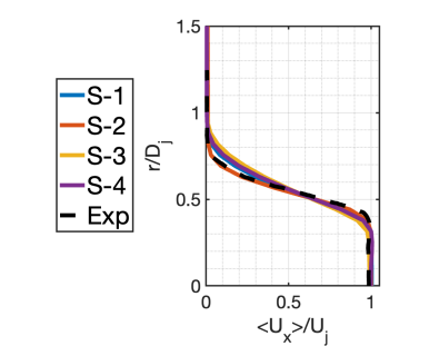
(a)

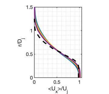
(b)

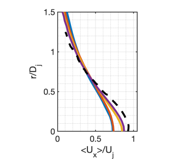
(c)

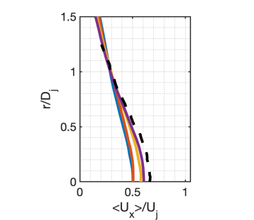
(d)

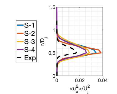
(e)

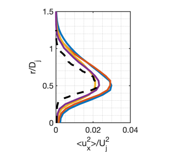
(f)

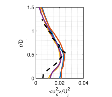
(g)

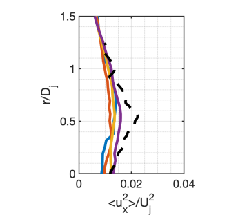
(h)

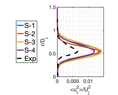
(i)

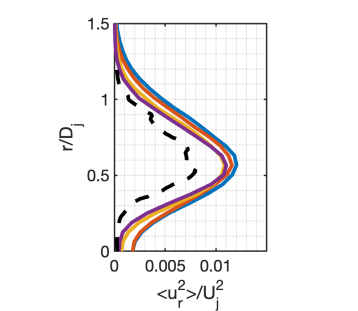
(j)

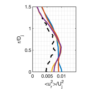
(k)

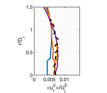
(l)

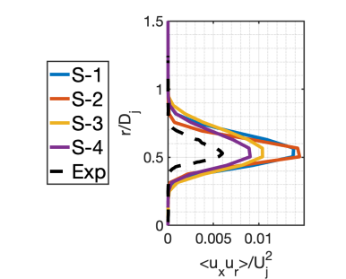
(m)

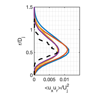
(n)

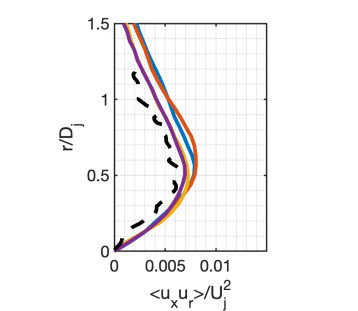
(o)

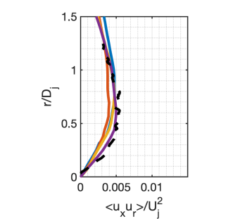
(p)

Figure 13: Profiles of mean longitudinal velocity component, RMS of longitudinal velocity fluctuation, RMS of radial velocity fluctuation, and mean shear stress tensor component (from top to bottom) at four streamwise positions $x/D_{j}=2.5$, $x/D_{j}=5.0$, $x/D_{j}=10.0$, and $x/D_{j}=15.0$ (from left to right).

5.5 Power Spectral Density

The velocity spectra analysis is performed through the power spectral density (PSD), Fig. 14, of the longitudinal velocity component fluctuation, Fig. 14a, and the radial velocity component fluctuation, Fig. 14b. The velocity spectra results are obtained in the same four streamwise positions of the radial analysis, $x/D_{j}=2.5$, $x/D_{j}=5.0$, $x/D_{j}=10.0$, and $x/D_{j}=15.0$, and they are all performed in the jet lipline $r/D_{j}=0.5$. The experimental reference is available for the last three sections. The charts show a cumulative shift of $20dB$ starting in the second position, $x/D_{j}=5.0$, to distinguish between the data in each section. Due to the limited acquisition frequency of the experimental apparatus, the experimental reference is only available to a maximum Strouhal number of $0.4$. It is possible to observe that for the positions $x/D_{j}=5.0$ and $x/D_{j}=10.0$, the PSD from all simulations is similar to the experimental data in the range of the experimental reference. In the last section, at $x/D_{j}=15.0$, for both velocity components, the spectra of the S-1 and S-2 simulations detach from the experimental data inside the range of experimental reference. A clear trend is present when comparing the data of the four numerical simulations in the available frequency range. The velocity spectra from the S-1 simulation present an abrupt power reduction in frequencies inside the experimental range. The S-2 simulation presents the same abrupt power reduction of the velocity spectra in frequencies slightly higher than those of the S-1 simulation. The power reduction of the velocity spectra from the S-3 and S-4 simulations occurs at higher frequencies than the S-1 and S-2 simulations. For the first two positions analyzed, in the range of the data, it is difficult to define the initial position of the PSD reduction from the S-4 simulation, which presents the best velocity spectra with larger power spectral values than the other simulations at large frequencies. In the first position, at $x/D_{j}=2.5$, the S-1 and S-2 simulations present a peak value of the velocity spectra close to a Strouhal number of $0.5$. This peak value can be associated with the late transition in the two simulations.

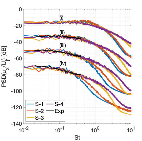
(a) PSD from the longitudinal velocity fluctuation.

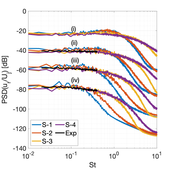
(b) PSD from the radial velocity fluctuation.

Figure 14: Power spectral density (PSD) of the velocity fluctuation at the lipline in four longitudinal positions: $x/D_{j}=2.5$ (i), $x/D_{j}=5.0$ (ii), $x/D_{j}=10.0$ (iii) and $x/D_{j}=15.0$ (iv). A cumulative value of $20dB$ is subtracted from the results of each station, starting at $x/D_{j}=5.0$ to allow the distinction between the velocity spectrum results in the same chart.

6 Concluding Remarks

In the present work, the impacts of hp resolution on large-eddy simulations of supersonic jet flows are investigated within the framework of the discontinuous Galerkin spectral element method, implemented in the open-source FLEXI solver. The simulations employed three computational meshes with two polynomial options to represent the numerical solution, leading to schemes with second- and third-order accurate spatial discretizations. The ensemble of numerical meshes and polynomials are employed in four simulations, with degrees of freedom from $50\times 10^{6}$ to $410\times 10^{6}$. The calculations are compared to experimental data.

The qualitative investigation of the instantaneous velocity and pressure contours showed that the simulations with high resolution could reproduce small flow features in the mixing layer and the region of the jet potential core. The highest-resolution simulation produced better-defined shock waves than the simulations with less resolution. Employing a third-order accurate spatial discretization scheme led to improvements when employed in different meshes with the same number of degrees of freedom and in the same numerical mesh. The comparison of mean velocity profiles showed that the highly-resolved simulations produced longer jet potential cores when compared to simulations with smaller resolutions. The root mean square value of velocity fluctuation indicates anticipation of the development of the mixing layer, which also presents a small spreading rate. The mean pressure contours showed an improved capacity to reproduce the shock structure in the jet interior with increased resolution.

The numerical data are compared with experimental data in terms of the velocity profiles at the jet centerline, jet lipline, and radial profiles in four streamwise positions. The velocity profiles at the centerline indicate a monotone improvement toward the experimental reference with the increasing resolution of the simulations. The monotone trend is observed for both mean velocity and root mean square values of velocity fluctuation distributions. In the jet lipline, the increase in the resolution of the simulations produced mean velocity values with a better agreement with experimental data. However, the root mean square values of the velocity fluctuation distributions distance themselves from the experimental reference. This behavior is attributed to the simplicity of the inlet profile imposed in the jet inlet condition, i.e., that the flow entering the domain is inviscid. The larger resolution of the simulations produces an anticipation of the development of the mixing layer, which is observed by a sudden change in the velocity fluctuation distribution slope. The highly-resolved simulation presentes the slope change occurring closer to the jet inlet section than the simulations with lower resolution. This behavior is not observed in the experimental reference.

Power spectral densities are calculated for the longitudinal and radial velocity signals in four streamwise positions in the jet lipline. The last three positions are compared with experimental data. The data acquisition frequency of the experiment restricted the comparison to low-frequencies, in which there is a good match of all numerical results with the experimental reference. When the comparison is extended to the frequencies available only from the numerical simulations, a monotone improvement is observed with the increase in the resolution of the simulations, represented by the larger power in the high frequencies.

In general, the most refined simulation, which employed the mesh with improved topology and a larger number of elements, $15.4\times 10^{6}$ elements, with a third-order accurate spatial discretization generated the best results when compared to the experimental reference. Such simulation has reproduced, with the highest quality, the different structures present in the flow, visualized by a diversity of velocity and pressure contours. The differences between the numerical simulation and experimental references are mostly correlated to the simple inviscid profile employed in the jet inlet condition that could not represent the aspects present in the experimental tests. The results obtained from the work show that the discontinuous Galerkin spectral element method is an interesting tool to the simulation of supersonic free jet flows. The work suggests a mesh topology, with a description of the element size distribution, and indicates an adequate polynomial resolution that together are capable of solving the large-eddy simulations of free jet flows with good accuracy. The present research could also profit from data of direct numerical simulation of the same supersonic jet flow configuration. Such effort could generate complete turbulent kinetic energy spectra which, in turn, would provide reference results that would allow a more precise indication of the portion of the spectrum which is actually being resolved by the present large eddy simulations. Clearly, however, such an effort is a quite demanding endeavor and requires adequate computational resources.

References

- \bibcommenthead
- Woodmansee et al. [2004] Woodmansee, M.A., Iyer, V., Dutton, J.C., Lucht, R.P.: Nonintrusive pressure and temperature measurements in an underexpanded sonic jet flowfield. AIAA Journal 42(6), 1170–1180 (2004) https://doi.org/10.2514/1.10418
- Bridges and Wernet [2008] Bridges, J., Wernet, M.P.: Turbulence associated with broadband shock noise in hot jets. In: Proceedings of the 29th AIAA Aeroacoustics Conference, AIAA Paper No. 2008-2834, Vancouver, British Columbia, Canada, pp. 1–21 (2008). https://doi.org/10.2514/6.2008-2834
- Morris and Zaman [2010] Morris, P.J., Zaman, K.B.M.Q.: Velocity measurements in jets with application to noise source modeling. Journal of Sound and Vibration 329, 394–414 (2010) https://doi.org/10.1016/j.jsv.2009.09.024
- Bogey and Bailly [2010] Bogey, C., Bailly, C.: Influence of nozzle-exit boundary-layer conditions on the flow and acoustic fields of initially laminar jets. Journal of Fluid Mechanics 663, 507–538 (2010) https://doi.org/%****␣sn-article.bbl␣Line␣100␣****10.1017/S0022112010003605
- DeBonis [2017] DeBonis, J.R.: Prediction of turbulent temperature fluctuations in hot jets. In: Proceedings of the 23th AIAA Computational Fluid Dynamics Conference, AIAA Paper No. 2017-0610, Denver, CO, pp. 1–25 (2017). https://doi.org/10.2514/6.2017-3610
- Brès et al. [2017] Brès, G.A., Ham, F.E., Nichols, J.W., Lele, S.K.: Unstructured large-eddy simulations of supersonic jets. AIAA Journal 55(4), 1164–1184 (2017) https://doi.org/10.2514/1.J055084
- Junqueira-Junior et al. [2018] Junqueira-Junior, C., Yamouni, S., Azevedo, J.L.F., Wolf, W.R.: Influence of different subgrid-scale models in low-order LES of supersonic jet flows. Journal of the Brazilian Society of Mechanical Sciences and Engineering 40(258), 1–29 (2018) https://doi.org/10.1007/s40430-018-1182-9
- Abreu et al. [2022] Abreu, D.F., Junqueira-Junior, C.A., Dauricio, E.T., Azevedo, J.L.F.: Study on the resolution of large-eddy simulations for supersonic jet flows. In: Proceedings of the AIAA Aviation 2022 Forum, AIAA Paper No. 2022-3327, Chicago, IL, pp. 1–16 (2022). https://doi.org/10.2514/6.2022-3327
- Zhang et al. [2015] Zhang, Y., Chen, H., Zhang, M., Zhang, M., Li, Z., Fu, S.: Performance prediction of conical nozzle using Navier-Stokes computation. Journal of Propulsion and Power 31(1), 192–203 (2015) https://doi.org/10.2514/1.B35164
- Pope [2000] Pope, S.B.: Turbulent Flows, 1st edn. Cambridge University Press, Cambridge, UK (2000)
- Bodony and Lele [2008] Bodony, D.J., Lele, J.K.: Current status of jet noise predicitions using large-eddy simulation. AIAA Journal 46(2), 364–380 (2008) https://doi.org/10.2514/1.24475
- Bogey et al. [2011] Bogey, C., Marsden, O., Bailly, C.: Large-eddy simulation of the flow and acoustic fields of a Reynolds number subsonic jet with tripped exit boundary layers. Physics of Fluids 23(035104), 1–20 (2011) https://doi.org/10.1063/1.3555634
- Yang et al. [2020] Yang, S., Yi, P., Habchi, C.: Real-fluid injection modeling and LES simulation of the ECN spray A injector using a fully compressible two-phase flow approach. International Journal of Multiphase Flow 122(103145), 1–21 (2020) https://doi.org/10.1016/j.ijmultiphaseflow.2019.103145
- Pradhan and Ghosh [2023] Pradhan, S., Ghosh, S.: LES of compressible round jet impinging on a flat plate. In: Proceedings of the AIAA SciTech 2023 Forum, AIAA Paper No. 2023-2150, National Harbor, MD, pp. 1–10 (2023). https://doi.org/10.2514/6.2023-2150
- Deng et al. [2022] Deng, X., Jiang, Z.-h., Vincent, P., Xiao, F., Yan, C.: A new paradigm of dissipation-adjustable, multi-scale resolving schemes for compressible flows. Journal of Computational Physics 466(111287), 1–24 (2022) https://doi.org/10.1016/j.jcp.2022.111287
- Noah et al. [2021] Noah, K., Lien, F.-S., Yee, E.: Large-eddy simulation of subsonic turbulent jets using the compressible lattice Boltzmann method. International Journal of Numerical Methods in Fluids 93, 927–952 (2021) https://doi.org/10.1002/fld.4914
- Bogey and Marsden [2016] Bogey, C., Marsden, O.: Simulations of initially highly disturbed jets with experiment-like exit boundary layers. AIAA Journal 54(4), 1299–1312 (2016) https://doi.org/10.2514/1.J054426
- Faranosov et al. [2013] Faranosov, G.A., Goloviznin, V.M., Karabasov, S.A., Kondakov, V.G., Kopiev, V.F., Zaitsev, M.A.: CABARET method on unstructured hexahedral grids for jet noise computation. Computers & Fluids 88, 165–179 (2013) https://doi.org/10.1016/j.compfluid.2013.08.011
- Brès et al. [2018] Brès, G.A., Jordan, P., Jaunet, V., Le Rallic, M., Cavalieri, A.V.G., Towne, A., Lele, S.K., Colonius, T., Schmidt, O.T.: Importance of the nozzle-exit boundary-layer state in subsonic turbulent jets. Journal of Fluid Mechanics 851, 83–124 (2018) https://doi.org/10.1017/jfm.2018.476
- Lorteau et al. [2018] Lorteau, M., de la Llave Plata, M., Couaillier, V.: Turbulent jet simulation using high-order DG methods for aeroacoustic analysis. International Journal of Heat and Fluid Flow 70, 380–390 (2018) https://doi.org/10.1016/j.ijheatfluidflow.2018.01.012
- Lindblad et al. [2023] Lindblad, D., Sherwin, S.J., Cantwell, C.D., Lawrence, J.L.T., Proença, A.R., Ginard, M.M.: Large eddy simulations of isolated and installed jet noise using high-order discontinuous Galerkin method. In: Proceedings of the AIAA SciTech 2023 Forum, AIAA Paper No. 2023-1546, National Harbor, MD, pp. 1–21 (2023). https://doi.org/10.2514/6.2023-1546
- Mendez et al. [2012] Mendez, S., Shoeybi, M., Sharma, A., Ham, F.E., Lele, S.K., Moin, P.: Large-eddy simulations of perfectly expanded supersonic jets using an unstructured solver. AIAA Journal 50(5), 1103–1118 (2012) https://doi.org/10.2514/1.J051211
- Langenais et al. [2019] Langenais, A., Vuillot, F., Troyes, J., Bailly, C.: Accurate simulation of the noise generated by a hot supersonic jet including turbulence tripping and nonlinear acoustic propagation. Physics of Fluids 31(016105), 1–31 (2019) https://doi.org/10.1063/1.5050905
- Bogey [2021] Bogey, C.: Acoustic tones in the near-nozzle region of jets: Characteristics and variations between Mach numbers 0.5 and 2. Journal of Fluid Mechanics 921, 3 (2021) https://doi.org/10.1017/jfm.2021.426
- Junqueira-Junior et al. [2020] Junqueira-Junior, C., Azevedo, J.L.F., Panetta, J., Wolf, W.R., Yamouni, S.: On the scalability of CFD tool for supersonic jet flow configurations. Parallel Computing 93, 102620 (2020) https://doi.org/10.1016/j.parco.2020.102620
- Shen and Miller [2020] Shen, W., Miller, S.A.E.: Validation of a high-order large eddy simulation solver for acoustic prediction of supersonic jet flow. Journal of Theoretical and Computational Acoustics 28(3), 1950023 (2020) https://doi.org/10.1142/S2591728519500233
- Chauhan and Massa [2022] Chauhan, M., Massa, L.: Large-eddy simulations of supersonic jet noise with discontinuous Galerkin methods. AIAA Journal 60(3), 1451–1470 (2022) https://doi.org/10.2514/1.J060424
- Kopriva and Gassner [2010] Kopriva, D.A., Gassner, G.: On the quadrature and weak form choices in collocation type discontinuous Galerkin spectral element methods. Journal of Scientific Computing 44, 136–155 (2010) https://doi.org/10.1007/s10915-010-9372-3
- Hindenlang et al. [2012] Hindenlang, F., Gassner, G.J., Altmann, C., Beck, A., Staudenmaier, M., Munz, C.-D.: Explicit discontinuous Galerkin methods for unsteady problems. Computers & Fluids 61, 86–93 (2012) https://doi.org/10.1016/j.compfluid.2012.03.006
- Krais et al. [2021] Krais, N., Beck, A., Bolemann, T., Frank, H., Flad, D., Gassner, G., Hindenlang, F., Hoffmann, M., Juhn, T., Sonntag, M., Munz, C.-D.: FLEXI: A high order discontinuous Galerkin framework for hyperbolic-parabolic conservation laws. Computers & Mathematics with Applications 81, 186–219 (2021) https://doi.org/10.1016/j.camwa.2020.05.004
- Garnier et al. [2009] Garnier, E., Adams, N., Sagaut, P.: Large Eddy Simulation for Compressible Flows, 1st edn. Springer, Dordrecht, The Netherlands (2009)
- Vreman et al. [1995] Vreman, B., Geurts, B., Kuerten, H.: A priori tests of large eddy simulation of the compressible plane mixing layer. Journal of Engineering Mathematics 29, 299–327 (1995) https://doi.org/10.1007/BF00042759
- White [2006] White, F.M.: Viscous Fluid Flow, 3rd edn. McGraw-Hill Education, New York (2006)
- Smagorinsky [1963] Smagorinsky, J.: General circulation experiments with the primitive equations. Monthly Weather Review 91(3), 99–164 (1963) https://doi.org/10.1175/1520-0493(1963)091<0099:GCEWTP>2.3.CO;2
- Gassner and Beck [2013] Gassner, G.J., Beck, A.D.: On the accuracy of high-order discretizations for underresolved turbulence simulations. Theoretical and Computational Fluid Dynamics 27, 221–237 (2013) https://doi.org/10.1007/s00162-011-0253-7
- Gassner [2014] Gassner, G.J.: A kinetic energy preserving nodal discontinuous Galerkin spectral element method. International Journal for Numerical Methods in Fluids 76(1), 28–50 (2014) https://doi.org/10.1002/fld.3923
- Beck et al. [2014] Beck, A.D., Bolemann, T., Flad, D., Frank, H., Gassner, G.J., Hindenlang, F., Munz, C.-D.: High-order discontinuous Galerkin spectral element methods for transitional and turbulent flow simulations. International Journal for Numerical Methods in Fluids 76(8), 522–548 (2014) https://doi.org/10.1002/fld.3943
- Flad and Gassner [2017] Flad, D., Gassner, G.: On the use of kinetic energy preserving DG-schemes for large eddy simulation. Journal of Computational Physics 350, 782–795 (2017) https://doi.org/10.1016/j.jcp.2017.09.004
- Pirozzoli [2011] Pirozzoli, S.: Numerical methods for high-speed flows. Annual Review of Fluid Mechanics 43, 163–194 (2011) https://doi.org/0.1146/annurev-fluid-122109-160718
- Gassner et al. [2016] Gassner, G.J., Winters, A.R., Kopriva, D.A.: Split form nodal discontinuous Galerkin schemes with summation-by-parts property for the compressible Euler equations. Journal of Computational Physics 327, 39–66 (2016) https://doi.org/10.1016/j.jcp.2016.09.013
- Dauricio and Azevedo [2021] Dauricio, E.T.V., Azevedo, J.L.F.: Large eddy simulations of turbulent channel flows using split form DG schemes. In: Proceedings of the AIAA SciTech 2021 Forum, AIAA Paper No. 2021-1209, Virtual Event, pp. 1–15 (2021). https://doi.org/10.2514/6.2021-1209
- Dauricio and Azevedo [2023] Dauricio, E.T.V., Azevedo, J.L.F.: A wall model for external laminar boundary layer flows applied to the wall-modeled LES framework. Journal of Computational Physics 484(112087), 1–21 (2023) https://doi.org/10.1016/j.jcp.2023.112087
- Harten and Hyman [1983] Harten, A., Hyman, J.M.: Self adjusting grid methods for one dimensional hyperbolic conservation laws. Journal of Computational Physics 50(2), 253–269 (1983) https://doi.org/10.1016/0021-9991(83)90066-9
- Bassi and Rebay [1997] Bassi, F., Rebay, S.: A high-order accurate discontinuous finite element method for the numerical solution of the compressible Navier-Stokes equations. Journal of Computational Physics 131(2), 267–279 (1997) https://doi.org/10.1006/jcph.1996.5572
- Kopriva [2009] Kopriva, D.A.: Implementing Spectral Methods for Partial Differential Equations, Algorithms for Scientists and Engineers, 1st edn. Springer, Dordrecht, The Netherlands (2009)
- Sonntag and Munz [2017] Sonntag, M., Munz, C.-D.: Efficient parallelization of a shock capturing for discontinuous Galerkin methods using finite volume sub-cells. Journal of Scientific Computing 70, 1262–1289 (2017) https://doi.org/10.1007/s10915-016-0287-5
- Jameson et al. [1981] Jameson, A., Schmidt, W., Turkel, E.: Numerical solution of the Euler equations by finite volume methods using Runge Kutta time stepping schemes. In: Proceedings of the 14th Fluid and Plasma Dynamics Conference, AIAA Paper No. 81-1259, Palo Alto, CA, pp. 1–17 (1981). https://doi.org/10.2514/6.1981-1259
- Hirsch [1990] Hirsch, C.: Numerical Computation of Internal and External Flows, Volume 2: Computational Methods for Inviscid and Viscous Flows, 1st edn. Wiley, Hoboken (1990)
- [49] Institute of Aerodynamics and Gas Dynamics, University of Stuttgart: FLEXI - High Performance Open Source CFD. Last accessed: 31 Jan. 2024. https://www.flexi-project.org
- Geuzaine and Remacle [2009] Geuzaine, C., Remacle, J.-F.: GMSH: A three-dimensional finite element mesh generator with built-in pre- and post-processing facilities. International Journal for Numerical Methods in Engineering 79(11), 1309–1331 (2009) https://doi.org/10.1002/nme.2579
- Flad et al. [2014] Flad, D.G., Frank, H.M., Beck, A.D., Munz, C.-D.: A discontinuous Galerkin spectral element method for the direct numerical simulation of aeroacoustics. In: Proceedings of the 20th AIAA/CEAS Aeroacoustics Conference, AIAA Paper No. 2014-2740, Atlanta, GA, pp. 1–10 (2014). https://doi.org/10.2514/6.2014-2740
- [52] IDRIS - Institute for Development and Resources in Intensive Scientific Computing: Jean Zay : HPE SGI 8600 computer. Last accessed: 31 Jan. 2024. http://www.idris.fr/eng/jean-zay/index.html