Resonances in nonlinear systems with a decaying chirped-frequency excitation and noise

Abstract. The influence of multiplicative white noise on the resonance capture of strongly nonlinear oscillatory systems under chirped-frequency excitations is investigated. It is assumed that the intensity of the perturbation decays polynomially with time, and its frequency grows according to a power low. Resonant solutions with a growing amplitude and phase, synchronized with the excitation, are considered. The persistence of such a regime in the presence of stochastic perturbations is discussed. In particular, conditions are described that guarantee the stochastic stability of the resonant modes on infinite or asymptotically large time intervals. The technique used is based on a combination of the averaging method, stability analysis and construction of stochastic Lyapunov functions. The proposed theory is applied to the Duffing oscillator with a chirped-frequency excitation and noise.

Keywords: damped perturbation, chirped-frequency, resonance, phase-locking, stochastic stability, Lyapunov function

Mathematics Subject Classification: 34F15, 34C15, 34E10, 34C29

Introduction

The present paper is devoted to the study of resonant phenomena in nonlinear pendulum-type systems. Resonance is usually referred to as the effect of increasing the energy of a system under the influence of the oscillating driving. This phenomenon is widely applicable in various fields: from acoustics and optics to electronics and mechanics (see, for example, [1, 2]). The persistent amplification of the amplitude occurs if the frequency of the driving is close to the natural frequency of the system. In the case of non-isochronous systems, perturbations with a chirped frequency turn out to be very effective [3, 4, 5]. In this case, the excitation frequency changes continuously with time. Resonant capture under small, slowly varying excitation with a chirped frequency has been studied in [6, 7, 8, 9]. In this paper, the presence of a small parameter is not assumed and a special class of chirped perturbations with a decaying intensity is considered.

Note that the influence of decaying perturbations on autonomous systems have been studied in many papers. In some cases, such perturbations can not disrupt the autonomous dynamics [10, 11, 12]. However, in the general case this cannot be guaranteed: the global properties of solutions to perturbed and unperturbed systems can differ significantly (see, for example, [13, 14]). Bifurcations in asymptotically autonomous systems have been studied in [15, 16, 17, 18]. The effect of decaying oscillatory perturbations with an asymptotically constant frequency on nonlinear autonomous systems in the plane was studied in [19, 20], where the dynamics near the equilibrium in resonance and non-resonance cases was discussed. The long-term asymptotic behaviour for solutions of similar but linear systems were investigated in [21, 22]. The decaying perturbations with chirped frequency were considered in [23, 24], where the conditions for the resonant capture far from the equilibrium were described. In this paper, we study the stability of such resonant regimes with respect to multiplicative stochastic perturbations of white noise type.

It is well known that even small stochastic perturbations can cause the trajectories of dynamical systems to leave any bounded domain [25]. Many papers (see, for example, [26, 27, 28, 29]) have studied the effect of autonomous stochastic perturbations on dynamical systems. Fading stochastic perturbations of scalar autonomous systems were considered in [30, 31, 32]. Bifurcations and asymptotic regimes for solutions in the vicinity of the equilibrium of near-Hamiltonian systems with decaying noise were discussed in [33, 34]. However, the influence of stochastic perturbations on the resonant capture far from the equilibrium has not been studied earlier. This is the subject of the present paper.

The paper is organized as follows. In Section 1, the statement of the problem is given, the class of perturbations is described, and a motivating example is presented. Preliminaries and auxiliary results that will be used below are contained in Section 2. The main results are presented in Section 3. The justification is provided in the subsequent sections. In particular, in Section 4 we prove the auxiliary results on the properties of a truncated system in the amplitude-angle variables. In Section 5 we construct the averaging transformation that simplifies the perturbed system in the first asymptotic terms at infinity in time. Then in Section 6, we consider a truncated system obtained from the simplified one by dropping the diffusion terms, and discuss the existence and stability of different long-term asymptotic regimes. In Section 7, we prove the persistence of the resonant mode in the full system by constructing suitable stochastic Lyapunov functions. In Section 8, the proposed theory is applied to the Duffing oscillator with various chirped perturbations and multiplicative noise. The paper concludes with a brief discussion of the results obtained.

1. Problem statement

Consider the system of Itô stochastic differential equations

(1) $$d\begin{pmatrix}x_{1}\\ x_{2}\end{pmatrix}=\begin{pmatrix}x_{2}\\ -U^{\prime}(x_{1})+t^{-\alpha}Q\left(x_{1},x_{2},S(t)\right)\end{pmatrix}dt+\begin{pmatrix}0\\ t^{-\gamma}\mu\sigma(x_{1},x_{2},S(t))\end{pmatrix}dw(t)$$

as $t\geq t_{0}\geq 1$ with $\alpha,\gamma,\mu\in\mathbb{R}_{+}$ and a polynomial potential

(2) $$U(x)\equiv\frac{x^{2h+2}}{2h+2}+\sum_{i=0}^{2h+1}u_{i}x^{i},\quad u_{i}\in\mathbb{R},\quad h\in\mathbb{Z}_{+},$$

where $w(t)$ is a Weiner process on a probability space $(\Omega,\mathfrak{A},\mathbb{P})$ and the function $S(t)\equiv st^{\beta+1}$ with $\beta,s\in\mathbb{R}_{+}$ corresponds to the phase of the excitation. It is assumed that the functions $Q(x_{1},x_{2},S)$ and $\sigma(x_{1},x_{2},S)$, defined for all $(x_{1},x_{2},S)\in\mathbb{R}^{3}$, are infinitely differentiable, do not depend on $\omega\in\Omega$ and have the following form:

(3) $$\begin{split}&Q(x_{1},x_{2},S)\equiv\sum_{i=0}^{p}\sum_{j=0}^{l}Q_{i,j}(S)x_{1}^{i}x_{2}^{j},\quad l,p\in\mathbb{Z},\quad 0\leq l\leq p\leq 2h+1,\\ &\sigma(x_{1},x_{2},S)\equiv\sum_{i=0}^{n}\sum_{j=0}^{m}\sigma_{i,j}(S)x_{1}^{i}x_{2}^{j},\quad n,m\in\mathbb{Z},\quad 0\leq n\leq p,\quad 0\leq m\leq l,\end{split}$$

where the coefficients $Q_{i,j}(S)$ and $\sigma_{i,j}(S)$ are $2\pi$-periodic with respect to $S$. Thus, (1) can be viewed as a pendulum-type system with a chirped-frequency excitation and multiplicative noise. The parameter $\mu$ with the decaying function $t^{-\gamma}$ are responsible for the noise intensity.

From [23] it follows that if $\mu=0$, then the deterministic system (1) may have a family of solutions with unlimitedly growing amplitude $|x_{1}(t)|+|x_{2}(t)|\to\infty$ as $t\to\infty$. This behaviour is associated with a resonance capture phenomenon. In this paper, we assume that $\mu\neq 0$ and study the effect of a noise on the stability of such solutions.

As an example, consider the perturbed Duffing oscillator

(4) $$dx_{1}=x_{2}\,dt,\quad dx_{2}=\left(x_{1}-x_{1}^{3}+t^{-\alpha}\mathcal{Q}x_{1}^{p}\cos S(t)\right)dt+t^{-\gamma}\mu x_{1}^{n}\cos S(t)\,dw(t),$$

with $\mathcal{Q}={\hbox{\rm const}}$. It can easily be checked that system (4) has the form of (1) with $U(x)\equiv x^{4}/4-x^{2}/2$, $h=1$, $l=m=0$, $Q(x_{1},x_{2},S)\equiv\mathcal{Q}x_{1}^{p}\cos S$ and $\sigma(x_{1},x_{2},S)\equiv x_{1}^{n}\cos S$. Note that all trajectories of the corresponding limiting autonomous system

$$\frac{dx_{1}}{dt}=x_{2},\quad\frac{dx_{2}}{dt}=x_{1}-x_{1}^{3}$$

are bounded (see Fig. 1). Moreover, the solutions with $H(x_{1}(t),x_{2}(t))\equiv E>0$, where $H(x_{1},x_{2})\equiv x_{1}^{4}/4+(x_{2}^{2}-x_{1}^{2})/2$, correspond to non-isochronous oscillations with a period $\tilde{T}(E)=\mathcal{O}(E^{-1/4})$ as $E\to\infty$. Numerical analysis of system (4) with $\mu=0$ shows that under certain conditions on the parameters of the chirped perturbation, the resonant solutions with an unboundedly growing amplitude $\rho(t)=[H(x_{1}(t),x_{2}(t))]^{1/4}$ take place (see Fig. 2, a, black curves). There are also non-resonant solutions with limited amplitude (see Fig. 2, a, grey curves). If $\mu\neq 0$, the stochastic perturbations may disrupt the resonant capture (see Fig. 2, b).

Thus, our goal is to find conditions under which the capture into the resonance persists in the stochastic system (1) with a high probability.

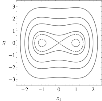
Figure 1. The level lines of $H(x_{1},x_{2})\equiv x_{1}^{4}/4+(x_{2}^{2}-x_{1}^{2})/2$. The solid curves correspond to $H(x_{1},x_{2})>0$.

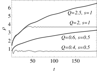
(a) $\mu=0$

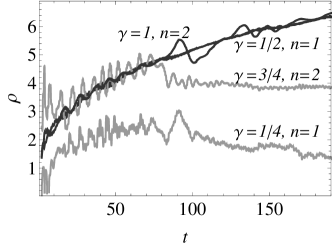
(b) $\mu=0.2$, $\mathcal{Q}=2.5$, $s=1$

Figure 2. The evolution of $\rho(t)\equiv[H(x_{1}(t),x_{2}(t))]^{1/4}$ for sample paths of solutions to system (4) with $\alpha=\beta=1/3$ and $p=0$.

2. Preliminaries and auxiliary results

Consider the limiting system

(5) $$\frac{dx_{1}}{dt}=\partial_{x_{2}}H(x_{1},x_{2}),\quad\frac{dx_{2}}{dt}=-\partial_{x_{1}}H(x_{1},x_{2}),\quad H(x_{1},x_{2})\equiv\frac{x_{2}^{2}}{2}+U(x_{1}).$$

It can easily be checked that there exists $\rho_{0}>0$ such that for every $\rho\geq\rho_{0}$ the level lines $\{(x_{1},x_{2})\in\mathbb{R}^{2}:H(x_{1},x_{2})=\rho^{2h+2}\}$ determine closed curves on the phase plane $(x_{1},x_{2})$ and correspond to $T(\rho)$-periodic solutions $\hat{x}_{1}(t;\rho)$, $\hat{x}_{2}(t;\rho)$ of system (5), where

$$T(\rho)\equiv\int\limits_{x_{-}(\rho)}^{x_{+}(\rho)}\frac{\sqrt{2}\,d\varsigma}{\sqrt{\rho^{2h+2}-U(\varsigma)}},$$

and $x_{-}(\rho)<0<x_{+}(\rho)$ are roots to the equation $U(x)=\rho^{2h+2}$ as $\rho>\rho_{0}$ such that $U^{\prime}(x_{\pm}(\rho))\neq 0$. For definiteness, suppose $\hat{x}_{1}(0;\rho)=x_{+}(\rho)$ and $\hat{x}_{2}(0;\rho)=0$. It follows from [23, Lemma 4.1] that

(6) $$\nu(\rho)\equiv\frac{2\pi}{T(\rho)},\quad\tilde{\nu}(\rho)\equiv\nu(\rho)\rho^{-h}\sim\sum_{k=0}^{\infty}\rho^{-k}\nu_{k},\quad\rho\to\infty$$

with constant coefficients $\nu_{k}={\hbox{\rm const}}$. In particular,

$$\nu_{0}=\frac{2\pi}{T_{0}},\quad T_{0}=(2h+2)^{\frac{1}{2h+2}}\int\limits_{-1}^{1}\frac{\sqrt{2}d\zeta}{\sqrt{1-\zeta^{2h+2}}},\quad\nu_{1}=0.$$

Define auxiliary $2\pi$-periodic functions $X_{1}(\varphi,\rho)=\hat{x}_{1}(\varphi/\nu(\rho),\rho)$ and $X_{2}(\varphi,\rho)=\hat{x}_{2}(\varphi/\nu(\rho),\rho)$. Then it follows from [23, Lemma 4.2] that

(7) $$\begin{split}X_{1}(\varphi,\rho)&\sim\rho\sum_{k=0}^{\infty}\rho^{-k}X_{1,k}(\varphi),\\ X_{2}(\varphi,\rho)&\sim\rho^{h+1}\sum_{k=0}^{\infty}\rho^{-k}X_{2,k}(\varphi)\end{split}$$

as $\rho\to\infty$ with $2\pi$-periodic coefficients $X_{i,k}(\varphi)$, where the leading terms $X_{1,0}(\varphi)$ and $X_{2,0}(\varphi)$ satisfy the system

(8) $$\nu_{0}\partial_{\varphi}X_{1,0}=X_{2,0},\quad\nu_{0}\partial_{\varphi}X_{2,0}=-X_{1,0}^{2h+1},\quad\frac{X_{1,0}^{2h+2}}{2h+2}+\frac{X_{2,0}^{2}}{2}=1.$$

Note that the series in (6) and (7) are assumed to be asymptotic as $\rho\to\infty$ (see, for example, [35, §1]). We use the functions $X_{1}(\varphi,\rho)$, $X_{2}(\varphi,\rho)$ for rewriting system (1) in the amplitude-angle variables $(\rho,\varphi)$:

(9) $$x_{1}=X_{1}(\varphi,\rho),\quad x_{2}=X_{2}(\varphi,\rho).$$

From the identity $H(X_{1}(\varphi,\rho),X_{2}(\varphi,\rho))\equiv\rho^{2h+2}$ it follows that

$$\Delta(\rho):=\begin{vmatrix}\partial_{\varphi}X_{1}&\partial_{\rho}X_{1}\\ \partial_{\varphi}X_{2}&\partial_{\rho}X_{2}\end{vmatrix}=\frac{(2h+2)\rho^{2h+1}}{\nu(\rho)}\neq 0,\quad\rho\geq\rho_{0}.$$

Hence, the transformation (9) is invertible for all $\rho\geq\rho_{0}$ and $\varphi\in[0,2\pi)$. Denote by

(10) $$\rho=Y_{1}(x_{1},x_{2}),\quad\varphi=Y_{2}(x_{1},x_{2})$$

the inverse transformation to (9) and define the domain $\mathcal{D}(\rho_{0})=\{(x_{1},x_{2})\in\mathbb{R}^{2}:H(x_{1},x_{2})>\rho_{0}\}$. Then, we have the following:

Lemma 1.

Let assumptions (2) and (3) hold. Then, for all $(x_{1},x_{2})\in\mathcal{D}(\rho_{0})$ system (1) can be transformed into

(11) $$\begin{split}&d\rho=F_{1}(\rho,\varphi,S(t),t)\,dt+t^{-\gamma}\mu c_{1}(\rho,\varphi,S(t),t)\,dw(t),\\ &d\varphi=\left(\nu(\rho)+F_{2}(\rho,\varphi,S(t),t)\right)dt+t^{-\gamma}\mu c_{2}(\rho,\varphi,S(t),t)\,dw(t),\end{split}$$

with $F_{i}(\rho,\varphi,S,t)\equiv t^{-\alpha}f_{i}(\rho,\varphi,S)+t^{-2\gamma}g_{i}(\rho,\varphi,S)$, $i\in\{1,2\}$, where

$$f_{i}(\rho,\varphi,S)\equiv Q(X_{1}(\varphi,\rho),X_{2}(\varphi,\rho),S)\partial_{x_{2}}Y_{i}(X_{1}(\varphi,\rho),X_{2}(\varphi,\rho)),$$

$$g_{i}(\rho,\varphi,S)\equiv\frac{\mu^{2}}{2}\sigma^{2}(X_{1}(\varphi,\rho),X_{2}(\varphi,\rho),S)\partial^{2}_{x_{2}}Y_{i}(X_{1}(\varphi,\rho),X_{2}(\varphi,\rho)),$$

$$c_{i}(\rho,\varphi,S)\equiv\sigma(X_{1}(\varphi,\rho),X_{2}(\varphi,\rho),S)\partial_{x_{2}}Y_{i}(X_{1}(\varphi,\rho),X_{2}(\varphi,\rho)).$$

Moreover, for every $i\in\{1,2\}$ the functions

$$\tilde{f}_{i}(\rho,\varphi,S)\equiv f_{i}(\rho,\varphi,S)\rho^{-(a+2-i)},\quad\tilde{g}_{i}(\rho,\varphi,S)\equiv g_{i}(\rho,\varphi,S)\rho^{-(2b+2-i)},$$

$$\tilde{c}_{i}(\rho,\varphi,S)\equiv c_{i}(\rho,\varphi,S)\rho^{-(b+2-i)}$$

have following asymptotic expansions:

(12) $$\begin{split}&\displaystyle\tilde{f}_{i}(\rho,\varphi,S)\sim\sum_{k=0}^{\infty}\rho^{-k}f_{i,k}(\varphi,S),\quad\displaystyle\tilde{g}_{i}(\rho,\varphi,S)\sim\sum_{k=0}^{\infty}\rho^{-k}g_{i,k}(\varphi,S),\\ &\displaystyle\tilde{c}_{i}(\rho,\varphi,S)\sim\sum_{k=0}^{\infty}\rho^{-k}c_{i,k}(\varphi,S)\end{split}$$

as $\rho\to\infty$ with $2\pi$-periodic coefficients $f_{i,k}(\varphi,S)$, $g_{i,k}(\varphi,S)$ and $c_{i,k}(\varphi,S)$. In particular,

$$\begin{pmatrix}f_{1,0}(\varphi,S)\\ f_{2,0}(\varphi,S)\end{pmatrix}\equiv\frac{\nu_{0}Q_{p,l}(S)}{2(h+1)}(X_{1,0}(\varphi))^{p}(X_{2,0}(\varphi))^{l}\begin{pmatrix}\partial_{\varphi}X_{1,0}(\varphi)\\ -X_{1,0}(\varphi)\end{pmatrix},$$

$$\begin{pmatrix}g_{1,0}(\varphi,S)\\ g_{2,0}(\varphi,S)\end{pmatrix}\equiv-\frac{(\mu\nu_{0}\sigma_{n,m}(S))^{2}}{8(h+1)^{2}}(X_{1,0}(\varphi))^{2n}(X_{2,0}(\varphi))^{2m}\begin{pmatrix}h(\partial_{\varphi}X_{1,0}(\varphi))^{2}+X_{1,0}(\varphi)\partial^{2}_{\varphi}X_{1,0}(\varphi)\\ -(h+2)X_{1,0}(\varphi)\partial_{\varphi}X_{1,0}(\varphi)\end{pmatrix},$$

$$\begin{pmatrix}c_{1,0}(\varphi,S)\\ c_{2,0}(\varphi,S)\end{pmatrix}\equiv\frac{\nu_{0}\sigma_{n,m}(S)}{2(h+1)}(X_{1,0}(\varphi))^{n}(X_{2,0}(\varphi))^{m}\begin{pmatrix}\partial_{\varphi}X_{1,0}(\varphi)\\ -X_{1,0}(\varphi)\end{pmatrix}.$$

Note that the limiting system corresponding to (11) has the following form: $d\varrho/dt=0$, $d\phi/dt=\nu(\varrho)$. Consider the resonance condition

(13) $$\nu(\varrho)=\varkappa^{-1}S^{\prime}(t),$$

where $\varkappa\in\mathbb{Z}_{+}$ corresponds to the resonance order. From (6) it follows that there exists $\tilde{\rho}_{0}>\rho_{0}$ such that $\nu(\varrho)>0$ and $\nu^{\prime}(\varrho)>0$ for all $\varrho\geq\tilde{\rho}_{0}$. Hence, for all $\varkappa\in\mathbb{Z}_{+}$ there exists $\hat{t}_{0}>t_{0}$ such that equation (13) has a smooth solution $\varrho_{\varkappa}(t)\geq\tilde{\rho}_{0}$ defined for all $t\geq\hat{t}_{0}$. Define $z(t)\equiv\varrho_{\varkappa}(t)t^{-{\beta}/{h}}$, then the following asymptotic expansion holds:

$$z(t)\sim\sum_{k=0}^{\infty}z_{k}t^{-\frac{k\beta}{h}},\quad t\to\infty,\quad z_{k}={\hbox{\rm const}},\quad z_{0}=\left(\frac{s(\beta+1)}{\nu_{0}\varkappa}\right)^{\frac{1}{h}},\quad z_{1}=-\frac{\nu_{1}}{h\nu_{0}}.$$

Hence, $\varrho_{\varkappa}(t)\sim t^{{\beta}/{h}}z_{0}$ as $t\to\infty$. Define the parameters

$$a=p+(l-1)(h+1),\quad b=n+(m-1)(h+1),$$

$$\mathcal{M}_{1}=-\alpha+\frac{a\beta}{h},\quad\mathcal{M}_{2}=-2\gamma+\frac{2b\beta}{h},\quad\mathcal{M}=\max\left\{\mathcal{M}_{1},\mathcal{M}_{2}\right\},$$

(14) $$A=\frac{1}{2}\left(\beta-\mathcal{M}\right),\quad B=\beta+1,\quad C=\frac{1}{2}\left(\beta-\min\left\{\mathcal{M}_{1},\mathcal{M}_{2}\right\}\right),$$

and consider the following axillary system, which is obtained from (11) by dropping the stochastic parts:

(15) $$\frac{d\varrho}{dt}=F_{1}(\varrho,\phi,S(t),t),\quad\frac{d\phi}{dt}=\nu(\varrho)+F_{2}(\varrho,\phi,S(t),t).$$

The following lemma describes the necessary condition for the existence of resonant refimes in the truncated system:

Lemma 2.

Let system (15) has solutions with asymptotics $\varrho(t)\sim\varrho_{\varkappa}(t)$, $\phi(t)\sim\varkappa^{-1}S(t)$ as $t\to\infty$, then

(16) $$-1\leq\mathcal{M}<\beta.$$

Thus, if the condition (16) is violated, the resonant solutions with unlimitedly growing amplitude and phase, synchronized with pumping, do not arise. We further assume that this condition is satisfied, and study the stability of such solutions with respect to white noise perturbations.

3. Main results

Consider the additional assumption on the parameters

(17) $$3\mathcal{M}_{1}-2\mathcal{M}_{2}\geq\beta.$$

Combining this with (16), we see that $\mathcal{M}_{1}>\mathcal{M}_{2}$, $\mathcal{M}=\mathcal{M}_{1}$, $A=(\beta-\mathcal{M}_{1})/2$, $C=(\beta-\mathcal{M}_{2})/2$, $B\geq 2A>0$ and $C\geq 3A/2$. Let us set

$$\langle f(\zeta)\rangle_{\varkappa\zeta}:=\frac{1}{2\pi\varkappa}\int\limits_{0}^{2\pi\varkappa}f(\zeta)\,d\zeta,\quad\{f(\zeta)\}_{\varkappa\zeta}:=f(\zeta)-\langle f(\zeta)\rangle_{\varkappa\zeta}.$$

Then, we have the following:

Theorem 1.

Let assumptions (2), (3), (16), and (17) hold. Then, for all $\varkappa\in\mathbb{Z}_{+}$ there exist $\tilde{t}_{0}>t_{0}$, $\tilde{\rho}_{0}\geq\rho_{0}$, $R_{0}>0$ and the chain of transformations $(x_{1},x_{2},t)\mapsto(\rho,\varphi,t)\mapsto(r,\theta,\tau)\mapsto(R,\Theta,\tau)$,

$$x_{1}(t)=X_{1}(\varphi(t),\rho(t)),\quad x_{2}(t)=X_{2}(\varphi(t),\rho(t)),$$

(18) $$\rho(t)=\varrho_{\varkappa}(t)\left(1+t^{-A}r(\tau)\right),\quad\varphi(t)=\varkappa^{-1}S(t)+\theta(\tau),\quad\tau=\frac{t^{B}}{B},$$

$$r(\tau)=R(\tau)+\tau^{-\frac{A}{B}}\tilde{Z}_{1}(R(\tau),\Theta(\tau),\zeta(\tau),\tau),\quad\theta(\tau)=\Theta(\tau)+\tau^{-\frac{A}{B}}\tilde{Z}_{2}(R(\tau),\Theta(\tau),\zeta(\tau),\tau),$$

with some smooth functions $\tilde{Z}_{i}(R,\Theta,\zeta,\tau)$ such that for all $t\geq\tilde{t}_{0}$ and $(x_{1},x_{2})\in\mathcal{D}(\tilde{\rho}_{0})$ system (1) can be transformed into

(19) $$\begin{split}&dR=\Lambda_{1}(R,\Theta,\zeta(\tau),\tau)\,d\tau+\tau^{-\frac{C-A}{B}}\mu\eta_{1}(R,\Theta,\zeta(\tau),\tau)\,d\tilde{w}(\tau),\\ &d\Theta=\Lambda_{2}(R,\Theta,\zeta(\tau),\tau)\,d\tau+\tau^{-\frac{C}{B}}\mu\eta_{2}(R,\Theta,\zeta(\tau),\tau)\,d\tilde{w}(\tau),\end{split}$$

where $\tilde{w}(\tau)$ is a Wiener process on a probabiluty space $(\Omega,\mathfrak{A},\mathbb{P})$, $\zeta(\tau)\equiv S((B\tau)^{\frac{1}{B}})$,

(20) $$\begin{split}\Lambda_{1}(R,\Theta,\zeta,\tau)\equiv&\sum_{K\in\{A,B-A,2A,B,2C-A\}}\tau^{-\frac{K}{B}}\Lambda_{1,K}(R,\Theta,\tau)+\tilde{\Lambda}_{1}(R,\Theta,\zeta,\tau),\\ \Lambda_{2}(R,\Theta,\zeta,\tau)\equiv&\sum_{K\in\{A,2A\}}\tau^{-\frac{K}{B}}\Lambda_{2,K}(R,\Theta,\tau)+\tilde{\Lambda}_{2}(R,\Theta,\zeta,\tau).\end{split}$$

The functions $\Lambda_{i}(R,\Theta,\zeta,\tau)$, $\eta_{i}(R,\Theta,\zeta,\tau)$, $\tilde{Z}_{i}(R,\Theta,\zeta,\tau)$ are $2\pi$-periodic in $\Theta$ and $2\pi\varkappa$-periodic in $\zeta$. Moreover, the following estimates hold:

$$\Lambda_{i,K}(R,\Theta,\tau)=\langle\mathcal{F}_{i,K}(R,\Theta,\zeta,\tau)\rangle_{\varkappa\zeta}+\delta_{i,1}\delta_{K,2A}\mathcal{O}(\tau^{-\frac{A}{B}})+\delta_{i,1}\delta_{K,2C-A}\mathcal{O}(\tau^{-\frac{2A}{B}}),$$

$$\tilde{Z}_{i}(R,\Theta,\zeta,\tau)=\mathcal{O}(1),\quad\eta_{i}(R,\Theta,\zeta,\tau)=\mathcal{O}(1),\quad\tilde{\Lambda}_{i}(R,\Theta,\zeta,\tau)=\mathcal{O}(\tau^{-\frac{3A}{B}})$$

as $\tau\to\infty$ uniformly for all $|R|\leq R_{0}$ and $(\Theta,\zeta)\in\mathbb{R}^{2}$, where the functions $\mathcal{F}_{i,K}(r,\theta,\zeta,\tau)$ are defined by (32).

Here, $\delta_{i,j}$ is the Kronecker delta. Note that (17) is equivalent to the inequality $C\geq 3A/2$. If the opposite inequality holds, then the diffusion coefficients in (19) become leading in the long-term dynamics as $\tau\to\infty$. This case requires a special attention and is not discussed here.

Consider the truncated deterministic system corresponding to (19)

(21) $$\frac{dR}{d\tau}=\Lambda_{1}(R,\Theta,\zeta(\tau),\tau),\quad\frac{d\Theta}{d\tau}=\Lambda_{2}(R,\Theta,\zeta(\tau),\tau)$$

as $\tau\geq\tilde{\tau}_{0}$, where $\tilde{\tau}_{0}=\tilde{t}_{0}^{B}/B$. It follows from (20) and (32) that the functions $\Lambda_{1}(R,\Theta,\zeta,\tau)$ and $\Lambda_{2}(R,\Theta,\zeta,\tau)$ can be written as

$$\Lambda_{i}(R,\Theta,\zeta,\tau)\equiv\hat{\lambda}_{i}(R,\Theta,\tau)+\tilde{\lambda}_{i}(R,\Theta,\zeta,\tau),\quad i\in\{1,2\},$$

with

(22) $$\begin{split}\hat{\lambda}_{1}(R,\Theta,\tau)\equiv&\,\tau^{-\frac{A}{B}}\vartheta_{1,A}(\Theta,\tau)+\tau^{-\frac{B-A}{B}}\chi_{1,B-A}(\tau)\\ &+\tau^{-\frac{2A}{B}}\vartheta_{1,2A}(\Theta,\tau)R+\tau^{-1}\chi_{1,B}(\tau)R+\tau^{-\frac{2C-A}{B}}\vartheta_{1,2C-A}(\Theta,\tau),\\ \hat{\lambda}_{2}(R,\Theta,\tau)\equiv&\,\tau^{-\frac{A}{B}}\chi_{2,A}(\tau)R+\tau^{-\frac{2A}{B}}\left(\vartheta_{2,2A}(\Theta,\tau)+\chi_{2,2A}(\tau)R^{2}\right),\end{split}$$

where

$$\vartheta_{1,A}(\Theta,\tau)\equiv \,B^{-\frac{A}{B}}(z(t))^{a}\left\langle\tilde{f}_{1}\left(\varrho_{\varkappa}(t),\varkappa^{-1}\zeta+\Theta,\zeta\right)\right\rangle_{\varkappa\zeta}\Big{|}_{t=(B\tau)^{\frac{1}{B}}},$$

$$\vartheta_{1,2A}(\Theta,\tau)\equiv \,(a+1)B^{-\frac{A}{B}}\vartheta_{1,A}(\Theta)+B^{-\frac{2A}{B}}(z(t))^{a}\varrho_{\varkappa}(t)\left\langle\partial_{\rho}\tilde{f}_{1}\left(\varrho_{\varkappa}(t),\varkappa^{-1}\zeta+\Theta,\zeta\right)\right\rangle_{\varkappa\zeta}\Big{|}_{t=(B\tau)^{\frac{1}{B}}},$$

$$\vartheta_{1,2C-A}(\Theta,\tau)\equiv \,B^{\frac{A-2C}{B}}(z(t))^{2b}\left\langle\tilde{g}_{1}\left(\varrho_{\varkappa}(t),\varkappa^{-1}\zeta+\Theta,\zeta\right)\right\rangle_{\varkappa\zeta}\Big{|}_{t=(B\tau)^{\frac{1}{B}}},$$

$$\vartheta_{2,2A}(\Theta,\tau)\equiv \,B^{-\frac{2A}{B}}(z(t))^{a}\left\langle\tilde{f}_{2}\left(\varrho_{\varkappa}(t),\varkappa^{-1}\zeta+\Theta,\zeta\right)\right\rangle_{\varkappa\zeta}\Big{|}_{t=(B\tau)^{\frac{1}{B}}},$$

$$\chi_{1,B-A}(\tau)\equiv \,-B^{\frac{A-B}{B}}\left(\frac{\beta}{h}+t(\log z(t))^{\prime}\right)\Big{|}_{t=(B\tau)^{\frac{1}{B}}},$$

$$\chi_{1,B}(\tau)\equiv \,\frac{A}{B}+B^{-\frac{A}{B}}\chi_{1,B-A}(\tau),$$

$$\chi_{2,A}(\tau)\equiv \,B^{-\frac{A}{B}}(z(t))^{h}\Big{\{}h\tilde{\nu}(\varrho_{\varkappa}(t))+\partial_{\rho}\tilde{\nu}\left(\varrho_{\varkappa}(t)\right)\varrho_{\varkappa}(t)\Big{\}}\Big{|}_{t=(B\tau)^{\frac{1}{B}}},$$

$$\chi_{2,2A}(\tau)\equiv \,B^{-\frac{2A}{B}}(z(t))^{h}\left\{\frac{h(h-1)\tilde{\nu}\left(\varrho_{\varkappa}(t)\right)}{2}+h\partial_{\rho}\tilde{\nu}\left(\varrho_{\varkappa}(t)\right)\varrho_{\varkappa}(t)+\frac{\partial_{\rho}^{2}\tilde{\nu}\left(\varrho_{\varkappa}(t)\right)(\varrho_{\varkappa}(t))^{2}}{2}\right\}\Big{|}_{t=(B\tau)^{\frac{1}{B}}}.$$

In this case, $\tilde{\lambda}_{i}(R,\Theta,\zeta,\tau)\equiv\Lambda_{i}(R,\Theta,\zeta,\tau)-\hat{\lambda}_{i}(R,\Theta,\tau)$. For every $i\in\{1,2\}$ the following estimate holds: $\tilde{\lambda}_{i}(R,\Theta,\zeta,\tau)=\mathcal{O}(\tau^{-{3A}/B})$ as $\tau\to\infty$ uniformly for all $|R|\leq R_{0}$ and $(\Theta,\zeta)\in\mathbb{R}^{2}$. It can easily be checked that the following asymptotic expansions hold:

(23) $$\begin{split}\vartheta_{i,K}(\Theta,\tau)&\sim\vartheta_{i,K,0}(\Theta)+\sum_{k=1}^{\infty}\tau^{-\frac{k\beta}{Bh}}\vartheta_{i,K,k}(\Theta),\\ \chi_{i,K}(\tau)&\sim\chi_{i,K,0}+\sum_{k=1}^{\infty}\tau^{-\frac{k\beta}{Bh}}\chi_{i,K,k}\end{split}$$

as $\tau\to\infty$, where $\vartheta_{i,K,k}(\Theta)$ are $2\pi$-periodic in $\Theta$ and $\chi_{i,K,k}$ are constants. In particular, the leading terms have the form

$$\vartheta_{1,A,0}(\Theta)\equiv \,B^{-\frac{A}{B}}z_{0}^{a}\left\langle f_{1,0}\left(\varkappa^{-1}\zeta+\Theta,\zeta\right)\right\rangle_{\varkappa\zeta},$$

$$\vartheta_{1,2A,0}(\Theta)\equiv \,(a+1)B^{-\frac{A}{B}}\vartheta_{1,A,0}(\Theta),$$

$$\vartheta_{1,2C-A,0}(\Theta)\equiv \,B^{\frac{A-2C}{B}}z_{0}^{2b}\left\langle g_{1,0}\left(\varkappa^{-1}\zeta+\Theta,\zeta\right)\right\rangle_{\varkappa\zeta},$$

$$\vartheta_{2,2A,0}(\Theta)\equiv \,B^{-\frac{2A}{B}}z_{0}^{a}\left\langle f_{2,0}\left(\varkappa^{-1}\zeta+\Theta,\zeta\right)\right\rangle_{\varkappa\zeta},$$

$$\chi_{1,B-A,0}= \,-B^{\frac{A-B}{B}}\frac{\beta}{h},$$

$$\chi_{1,B,0}= \,\frac{1}{B}\left(A-\frac{\beta}{h}\right),$$

$$\chi_{2,A,0}= \,B^{-\frac{A}{B}}z_{0}^{h}h\nu_{0},$$

$$\chi_{2,2A,0}= \,B^{-\frac{2A}{B}}\frac{z_{0}^{h}h(h-1)\nu_{0}}{2}.$$

It is clear that the long-term dynamics of the asymptotically autonomous system (21) depends on the properties of the leading terms of the right-hand sides as $\tau\to\infty$. With this in mind, define

(24) $$\mathcal{P}(\Theta) \equiv\vartheta_{1,A,0}(\Theta)+\delta_{B,2A}\chi_{1,B-A,0},$$

(25) $$J(\Theta) \equiv\vartheta_{1,2A,0}(\Theta)+\vartheta_{2,2A,0}^{\prime}(\Theta)+\delta_{B,2A}\chi_{1,B,0},$$

and consider the assumption

(26) $$\exists\,\Theta_{0}\in\mathbb{R}:\quad\mathcal{P}(\Theta_{0})=0,\quad\mathcal{P}^{\prime}(\Theta_{0})\neq 0.$$

Then, we have the following:

Lemma 3.

Let assumptions (16), (17) and (26) hold.

• If $\mathcal{P}^{\prime}(\Theta_{0})<0$ and $J(\Theta_{0})<0$, then there exists $\tau_{0}\geq\tilde{\tau}_{0}$ such that system (21) has an asymptotically stable solution $R_{\ast}(\tau)$, $\Theta_{\ast}(\tau)$ defined for all $\tau\geq\tau_{0}$. Moreover, $R_{\ast}(\tau)=o(1)$ and $\Theta_{\ast}(\tau)=\Theta_{0}+o(1)$ as $\tau\to\infty$.

• If $\mathcal{P}^{\prime}(\Theta_{0})<0$ and $J(\Theta_{0})>0$ or $\mathcal{P}^{\prime}(\Theta_{0})>0$, then there exists $\varepsilon_{\ast}>0$ such that for all $\delta\in(0,\varepsilon_{\ast})$ the solutions of system (21) with initial data $\sqrt{R^{2}(\tau_{\ast})+(\Theta(\tau_{\ast})-\Theta_{0})^{2}}=\delta$ and some $\tau_{\ast}\geq\tilde{\tau}_{0}$ exit from the domain $\{(R,\Theta)\in\mathbb{R}^{2}:\sqrt{R^{2}+(\Theta-\Theta_{0})^{2}}<\varepsilon_{\ast}\}$ in a finite time.

Thus, Lemma 3 guarantees the existence and stability of the phase-locking regime in the truncated system (21). Such solutions correspond to a resonant increase of the amplitude, $\rho(t)\sim\varrho_{\varkappa}(t)$, and to a synchronization of the system with the excitation, $\varphi(t)-\varkappa^{-1}S(t)\sim\Theta_{0}$ as $t\to\infty$. If (26) does not hold, we have the following:

Lemma 4.

Let assumptions (16), (17) hold and

(27) $$\mathcal{P}(\Theta)\neq 0\quad\forall\,\Theta\in\mathbb{R}.$$

Then, the solutions of system (21) exit from any bounded domain in a finite time.

This lemma describes the conditions for the phase drifting mode. In this case, the amplitude $\rho(t)$ and the phase $\varphi(t)$ of system can significantly differ from $\varrho_{\varkappa}(t)$ and $\varkappa^{-1}S(t)$ even in the absence of the stochastic perturbations.

Let us show that the phase-locking regime is preserved with a high probability in the full stochastic system (19). Define the function

$$d(\rho,\varphi,t)\equiv\sqrt{\left\{\left(\frac{\rho}{\varrho_{\varkappa}(t)}-1\right)t^{A}-R_{\ast}\left(\frac{t^{B}}{B}\right)\right\}^{2}+\left\{\varphi-\varkappa^{-1}S(t)-\Theta_{\ast}\left(\frac{t^{B}}{B}\right)\right\}^{2}}.$$

Then, we have

Theorem 2.

Let assumptions (2), (3), (16), (17), and (26) hold. If $\mathcal{P}^{\prime}(\Theta_{0})<0$ and $J(\Theta_{0})<0$, then for all $\varepsilon_{1}>0$, $\varepsilon_{2}>0$, $\epsilon\in(0,1)$ and $t_{\ast}\geq\tilde{t}_{0}$ there exist $\delta_{1}>0$ and $\delta_{2}>0$ such that the solution $\rho(t)$, $\varphi(t)$ of system (11) with initial data $d(\rho(t_{\ast}),\varphi(t_{\ast}),t_{\ast})<\delta_{1}$ and $0<\mu<\delta_{2}$ satisfies

(28) $$\mathbb{P}\left(\sup_{0<t-t_{\ast}\leq\tilde{\mathcal{T}}}d(\rho(t),\varphi(t),t)\geq\varepsilon_{1}\right)\leq\varepsilon_{2},$$

where

$$\tilde{\mathcal{T}}=\begin{cases}\displaystyle t_{\ast}\left(\mu^{-\frac{2(1-\epsilon)}{B}}-1\right),&\text{if}\quad C<A+\frac{B}{2},\\ \displaystyle t_{\ast}\left(\exp{\mu^{-\frac{2(1-\epsilon)}{B}}}-1\right),&\text{if}\quad C=A+\frac{B}{2},\\ \infty,&\text{if}\quad C>A+\frac{B}{2}.\end{cases}$$

Note that deviation estimates similar to (28) usually arise when studying the stability in probability [41, §5.3]. Besides, the stability on an asymptotically large time interval corresponds to some variant of a practical stability [42, §25].

Thus, Theorem 2 describes the condtions under which the stochastic perturbations do not destroy the resonant capture in system (1). Depending on the parameters of the system, the dynamics $\rho(t)\approx\varrho_{\varkappa}(t)$, $\varphi(t)\approx\varkappa^{-1}S(t)+\Theta_{0}$ is preserved with a high probability on infinite or asymptotically large time intervals as $\mu\to 0$. Combining this with Theorem 1, we see that the resonant behaviour occurs in system (11) such that

$$x_{1}(t)\approx t^{\frac{\beta}{h}}z_{0}X_{1,0}(\varphi(t)),\quad x_{2}(t)\approx t^{\frac{(h+1)\beta}{h}}z_{0}^{h+1}X_{2,0}(\varphi(t)),$$

where $X_{1,0}(\varphi)$ and $X_{2,0}(\varphi)$ are $2\pi$-periodic functions defined by (8).

4. Proof of auxiliary results

Proof of Lemma 1.

Applying Itô’s formula [36, §4.2] to (10), we see that in the new variables $(\rho,\varphi)$ system (1) takes the form (11). From the properties of the functions $X_{1}(\varphi,\rho)$ and $X_{2}(\varphi,\rho)$ it follows that

$$\partial_{x_{2}}\begin{pmatrix}Y_{1}\\ Y_{2}\end{pmatrix} \equiv\frac{1}{\Delta(\rho)}\begin{pmatrix}\partial_{\varphi}X_{1}\\ -\partial_{\rho}X_{1}\end{pmatrix},$$

$$\partial_{x_{2}}^{2}\begin{pmatrix}Y_{1}\\ Y_{2}\end{pmatrix} \equiv\frac{1}{\Delta(\rho)}\left(\partial_{\varphi}X_{1}\partial_{\rho}-\partial_{\rho}X_{1}\partial_{\varphi}\right)\frac{1}{\Delta(\rho)}\begin{pmatrix}\partial_{\varphi}X_{1}\\ -\partial_{\rho}X_{1}\end{pmatrix}.$$

Combing this with (3) and (7), we obtain (12). ∎

Proof of Lemma 2.

It follows from (12) that there exist $D>0$ and $\hat{\varrho}_{0}>\hat{\rho}_{0}$ such that

$$|f_{i}(\varrho,\phi,S)|\leq D\varrho^{a+2-i},\quad|g_{i}(\varrho,\phi,S)|\leq D\varrho^{2b+2-i}$$

for all $i\in\{1,2\}$, $\varrho\geq\hat{\varrho}_{0}$ and $(\varrho,\phi)\in\mathbb{R}^{2}$. Combining this with the first equation in (15), we obtain the following inequality for solutions:

(29) $$\left|\frac{d}{dt}\log\varrho(t)\right|\leq D\left(t^{-\alpha}(\varrho(t))^{a}+t^{-2\gamma}(\varrho(t))^{2b}\right).$$

It is not hard to check that

$$\left(\log\varrho_{\varkappa}(t)\right)^{\prime}\sim\frac{\beta}{h}t^{-1},\quad t^{-\alpha}(\varrho_{\varkappa}(t))^{a}\sim z_{0}^{a}t^{\mathcal{M}_{1}},\quad t^{-2\gamma}(\varrho_{\varkappa}(t))^{2b}\sim z_{0}^{2b}t^{\mathcal{M}_{2}},\quad t\to\infty.$$

Substituting these estimates into (29), we see that system (15) admits solutions with $\varrho(t)\sim\varrho_{\varkappa}(t)$ as $t\to\infty$ if $\mathcal{M}\geq-1$.

From the second equation in (15) it follows that

$$\frac{\phi(t)}{S(t)}-\varkappa^{-1}=\mathcal{O}\left(t^{\mathcal{M}-\beta}\right),\quad t\to\infty$$

for $\varrho(t)\sim\varrho_{\varkappa}(t)$. Since $\phi(t)/S(t)\to\varkappa^{-1}$ as $t\to\infty$, we get $\mathcal{M}<\beta$. ∎

5. Change of variables

5.1. Amplitude remainder and phase shift

Consider the change of variables (18) in system (11). Using Itô’s formula and the change of time formula for stochastic integrals [36, §8.5], we obtain

(30) $$\begin{split}&dr=\mathcal{F}_{1}(r,\theta,\zeta(\tau),\tau)\,d\tau+\tau^{-\frac{C-A}{B}}\mu\xi_{1}(r,\theta,\zeta(\tau),\tau)\,d\tilde{w}(\tau),\\ &d\theta=\mathcal{F}_{2}(r,\theta,\zeta(\tau),\tau)\,d\tau+\tau^{-\frac{C}{B}}\mu\xi_{2}(r,\theta,\zeta(\tau),\tau)\,d\tilde{w}(\tau),\end{split}$$

where the functions

$$\mathcal{F}_{1}\equiv \,t^{A+1-B}\left\{F_{1}\left(\varrho_{\varkappa}(t)(1+t^{-A}r),\varkappa^{-1}\zeta+\theta,\zeta,t\right)-\varrho_{\varkappa}^{\prime}(t)\right\}(\varrho_{\varkappa}(t))^{-1}$$

$$+t^{-B}r\left(A-t\left(\log\varrho_{\varkappa}(t)\right)^{\prime}\right)\Big{|}_{t=(B\tau)^{\frac{1}{B}}},$$

$$\mathcal{F}_{2}\equiv \,t^{1-B}\Big{\{}\nu\big{(}\varrho_{\varkappa}(t)(1+t^{-A}r)\big{)}-\varkappa^{-1}S^{\prime}(t)+F_{2}\left(\varrho_{\varkappa}(t)(1+t^{-A}r),\varkappa^{-1}\zeta+\theta,\zeta,t\right)\Big{\}}\Big{|}_{t=(B\tau)^{\frac{1}{B}}},$$

$$\xi_{1}\equiv \,t^{C-\gamma+\frac{1-B}{2}}B^{-\frac{C-A}{B}}c_{1}\left(\varrho_{\varkappa}(t)(1+t^{-A}r),\varkappa^{-1}\zeta+\theta,\zeta,t\right)(\varrho_{\varkappa}(t))^{-1}\Big{|}_{t=(B\tau)^{\frac{1}{B}}},$$

$$\xi_{2}\equiv \,t^{C-\gamma+\frac{1-B}{2}}B^{-\frac{C}{B}}c_{2}\left(\varrho_{\varkappa}(t)(1+t^{-A}r),\varkappa^{-1}\zeta+\theta,\zeta,t\right)\Big{|}_{t=(B\tau)^{\frac{1}{B}}}$$

are $2\pi$-periodic in $\theta$ and $2\pi\varkappa$-periodic in $\zeta$. Note that the right-hand sides of system (30) satisfy the following estimates:

(31) $$\begin{split}\mathcal{F}_{1}(r,\theta,\zeta,\tau)=&\sum_{K\in\{A,B-A,2A,2C-A,B\}}\tau^{-\frac{K}{B}}\mathcal{F}_{1,K}(r,\theta,\zeta,\tau)+\mathcal{O}(\tau^{-\frac{3A}{B}}),\\ \mathcal{F}_{2}(r,\theta,\zeta,\tau)=&\sum_{K\in\{A,2A\}}\tau^{-\frac{K}{B}}\mathcal{F}_{2,K}(r,\theta,\zeta,\tau)+\mathcal{O}(\tau^{-\frac{3A}{B}}),\\ \xi_{i}(r,\theta,\zeta,\tau)=&\,\xi_{i,0}(r,\theta,\zeta,\tau)+\mathcal{O}(\tau^{-\frac{A}{B}})\end{split}$$

as $\tau\to\infty$ uniformly for all $(\theta,\zeta)\in\mathbb{R}^{2}$ and $|r|\leq r_{0}$, where $r_{0}=(\tilde{\rho}_{0}/\rho_{0}-1)\hat{t}_{0}^{A}>0$,

(32) $$\begin{split}\mathcal{F}_{1,A}(r,\theta,\zeta,\tau)\equiv&\,B^{-\frac{A}{B}}(z(t))^{a}\tilde{f}_{1}\left(\varrho_{\varkappa}(t)(1+t^{-A}r),\varkappa^{-1}\zeta+\theta,\zeta\right)\Big{|}_{t=(B\tau)^{\frac{1}{B}}},\\ \mathcal{F}_{1,B-A}(r,\theta,\zeta,\tau)\equiv&\,-B^{\frac{A-B}{B}}\left(\frac{\beta}{h}+t(\log z(t))^{\prime}\right)\Big{|}_{t=(B\tau)^{\frac{1}{B}}},\\ \mathcal{F}_{1,2A}(r,\theta,\zeta,\tau)\equiv&\,rB^{-\frac{A}{B}}(a+1)\mathcal{F}_{1,A}(r,\theta,\zeta,\tau),\\ \mathcal{F}_{1,B}(r,\theta,\zeta,\tau)\equiv&\,r\left(\frac{A}{B}+B^{-\frac{A}{B}}\mathcal{F}_{1,B-A}(r,\theta,\zeta,\tau)\right),\\ \mathcal{F}_{1,2C-A}(r,\theta,\zeta,\tau)\equiv&\,B^{\frac{A-2C}{B}}(z(t))^{2b}\tilde{g}_{1}\left(\varrho_{\varkappa}(t)(1+t^{-A}r),\varkappa^{-1}\zeta+\theta,\zeta\right)\Big{|}_{t=(B\tau)^{\frac{1}{B}}},\\ \mathcal{F}_{2,A}(r,\theta,\zeta,\tau)\equiv&\,B^{-\frac{A}{B}}(z(t))^{h}\Big{\{}hr\tilde{\nu}(\varrho_{\varkappa}(t))+t^{A}\Big{(}\tilde{\nu}\big{(}\varrho_{\varkappa}(t)(1+t^{-A}r)\big{)}-\tilde{\nu}\big{(}\varrho_{\varkappa}(t)\big{)}\Big{)}\Big{\}}\Big{|}_{t=(B\tau)^{\frac{1}{B}}},\\ \mathcal{F}_{2,2A}(r,\theta,\zeta,\tau)\equiv&\,rB^{-\frac{2A}{B}}(z(t))^{h}\frac{h}{2}\Big{\{}(h-1)r\tilde{\nu}(\varrho_{\varkappa}(t))+2t^{A}\Big{(}\tilde{\nu}\big{(}\varrho_{\varkappa}(t)(1+t^{-A}r)\big{)}-\tilde{\nu}\big{(}\varrho_{\varkappa}(t)\big{)}\Big{)}\Big{\}}\\ &\,+B^{-\frac{2A}{B}}(z(t))^{a}\tilde{f}_{2}\left(\varrho_{\varkappa}(t)(1+t^{-A}r),\varkappa^{-1}\zeta+\theta,\zeta\right)\Big{|}_{t=(B\tau)^{\frac{1}{B}}},\\ \xi_{1,0}(r,\theta,\zeta,\tau)\equiv&\,B^{-\frac{C-A}{B}}(z(t))^{b}\tilde{c}_{1}\left(\varrho_{\varkappa}(t)(1+t^{-A}r),\varkappa^{-1}\zeta+\theta,\zeta\right)\Big{|}_{t=(B\tau)^{\frac{1}{B}}},\\ \xi_{2,0}(r,\theta,\zeta,\tau)\equiv&\,B^{-\frac{C}{B}}(z(t))^{b}\tilde{c}_{2}\left(\varrho_{\varkappa}(t)(1+t^{-A}r),\varkappa^{-1}\zeta+\theta,\zeta\right)\Big{|}_{t=(B\tau)^{\frac{1}{B}}}.\end{split}$$

Moreover, the following asymptotic expansions hold:

$$\mathcal{F}_{i,K}(r,\theta,\zeta,\tau)\sim\mathcal{F}_{i,K}^{0}(r,\theta,\zeta)+\sum_{j\geq 1,k\geq 0}\tau^{-\frac{j(\beta/h)+kA}{B}}\mathcal{F}_{i,K}^{j,k}(r,\theta,\zeta),$$

$$\xi_{i,0}(r,\theta,\zeta,\tau)\sim\mathcal{\xi}_{i,0}^{0}(r,\theta,\zeta)+\sum_{j\geq 1,k\geq 0}\tau^{-\frac{j(\beta/h)+kA}{B}}\xi_{i,0}^{j,k}(r,\theta,\zeta)$$

as $\tau\to\infty$ with time-independent coefficients $\mathcal{F}_{1,K}^{j,k}(r,\theta,\zeta)$ and $\xi_{i,0}^{j,k}(r,\theta,\zeta)$. In particular,

$$\mathcal{F}_{1,A}^{0} \equiv B^{-\frac{A}{B}}z_{0}^{a}f_{1,0}(\varkappa^{-1}\zeta+\theta,\zeta), \mathcal{F}_{2,A}^{0} \equiv rB^{-\frac{A}{B}}h\nu_{0}z_{0}^{h},$$

$$\mathcal{F}_{1,B-A}^{0} \equiv-B^{\frac{A-B}{B}}\frac{\beta}{h}, \mathcal{F}_{2,B-A}^{0} \equiv 0,$$

$$\mathcal{F}_{1,2A}^{0} \equiv rB^{-\frac{A}{B}}(a+1)\mathcal{F}_{1,A}^{0}, \mathcal{F}_{2,2A}^{0} \equiv B^{-\frac{2A}{B}}\left(h(h-1)\nu_{0}z_{0}^{h}\frac{r^{2}}{2}+f_{2,0}(\varkappa^{-1}\zeta+\theta,\zeta)z_{0}^{a}\right),$$

$$\mathcal{F}_{1,B}^{0} \equiv\frac{r}{B}\left(A-\frac{\beta}{h}\right), \mathcal{F}_{2,B}^{0} \equiv 0,$$

$$\mathcal{F}_{1,2C-A}^{0} \equiv B^{\frac{A-2C}{B}}z_{0}^{2b}g_{1,0}(\varkappa^{-1}\zeta+\theta,\zeta), \mathcal{F}_{2,2C-A}^{0} \equiv 0,$$

$$\xi_{1,0}^{0} \equiv B^{-\frac{C-A}{B}}z_{0}^{b}c_{1,0}(\varkappa^{-1}\zeta+\theta,\zeta), \xi_{2,0}^{0} \equiv B^{-\frac{C}{B}}z_{0}^{b}c_{2,0}(\varkappa^{-1}\zeta+\theta,\zeta).$$

5.2. Averaging

Note that the limiting system, corresponding to (30), has the form

$$\frac{dr}{d\tau}=0,\quad\frac{d\theta}{d\tau}=0,\quad\frac{d\zeta}{d\tau}=\varsigma,$$

where $\varsigma=sB>0$. In this case, $\zeta$ can be considered as a fast variable, and system (30) can be simplified by averaging the drift terms with respect to $\zeta$. Note that such averaging transformations are successfully used in problems with a small parameter [37, 38] and in studying the asymptotics of solutions to non-autonomous systems at infinity [39, 40]. Consider a near-identity transformation in the following form:

(33) $$\begin{split}&\tilde{R}(r,\theta,\zeta,\tau)\equiv\displaystyle r+\sum_{K\in\mathcal{X}}\tau^{-\frac{K}{B}}Z_{1,K}(r,\theta,\zeta,\tau),\\ &\tilde{\Theta}(r,\theta,\zeta,\tau)\equiv\displaystyle\theta+\sum_{K\in\mathcal{X}}\tau^{-\frac{K}{B}}Z_{2,K}(r,\theta,\zeta,\tau),\end{split}$$

where $\mathcal{X}:=\{A,B-A,2A,2(B-A),2C-A,B,B+2C-3A\}$. The coefficients $Z_{i,K}(r,\theta,\zeta,\tau)$, $i\in\{1,2\}$ are assumed to be periodic w.r.t. $\theta$ and $\zeta$ with zero means. These functions are chosen in such a way that the drift terms of system (19) written in the new variables

(34) $$R(\tau)=\tilde{R}(r(\tau),\theta(\tau),\zeta(\tau),\tau),\quad\Theta(\tau)=\tilde{\Theta}(r(\tau),\theta(\tau),\zeta(\tau),\tau)$$

do not depend explicitly on $\zeta(\tau)$ at least in the leading terms. By applying Itô’s formula [36, §4.2] to (34), we obtain

$$dR=\mathcal{L}\tilde{R}\,d\tau+\mu\left(\tau^{-\frac{C-A}{B}}\xi_{1}\partial_{r}+\tau^{-\frac{C}{B}}\xi_{2}\partial_{\theta}\right)\tilde{R}\,d\tilde{w}(\tau),$$

$$d\Theta=\mathcal{L}\tilde{\Theta}\,d\tau+\mu\left(\tau^{-\frac{C-A}{B}}\xi_{1}\partial_{r}+\tau^{-\frac{C}{B}}\xi_{2}\partial_{\theta}\right)\tilde{\Theta}\,d\tilde{w}(\tau),$$

where

$$\mathcal{L}:=\mathcal{F}_{1}\partial_{r}+\mathcal{F}_{2}\partial_{\theta}+\partial_{\tau}+\varsigma\partial_{\zeta}+\frac{\mu^{2}}{2}\tau^{-\frac{2(C-A)}{B}}\left(\xi_{1}^{2}\partial^{2}_{r}+2\tau^{-\frac{A}{B}}\xi_{1}\xi_{2}\partial_{r}\partial_{\theta}+\tau^{-\frac{2A}{B}}\xi_{2}^{2}\partial_{\theta}^{2}\right)$$

is the generator of the process defined by (30) (see, for example, [41, §3.3]). Calculating $\mathcal{L}\tilde{R}$ and $\mathcal{L}\tilde{\Theta}$, using (31) and (33), and comparing the result with (20), we obtain the following chain of equations:

(35) $$\varsigma\partial_{\zeta}Z_{i,K}=\Lambda_{i,K}(r,\theta,\tau)-\mathcal{F}_{i,K}(r,\theta,\zeta,\tau)+\tilde{\mathcal{F}}_{i,K}(r,\theta,\zeta,\tau),\quad K\in\mathcal{X},\quad i\in\{1,2\}.$$

It is assumed that

(36) $$\mathcal{F}_{2,B-A}\equiv\mathcal{F}_{2,B}\equiv\mathcal{F}_{2,2C-A}\equiv\mathcal{F}_{i,2(B-A)}\equiv\mathcal{F}_{i,B+2C-3A}\equiv 0.$$

The functions $\tilde{\mathcal{F}}_{i,K}(r,\theta,\zeta,\tau)$ are expressed through $\{Z_{i,k},\Lambda_{i,k}\}_{k<K}$. In particular,

(37) $$\begin{split}\tilde{\mathcal{F}}_{i,A}(r,\theta,\zeta,\tau)\equiv&\,0,\\ \tilde{\mathcal{F}}_{i,B-A}(r,\theta,\zeta,\tau)\equiv&\,0,\\ \tilde{\mathcal{F}}_{i,2A}(r,\theta,\zeta,\tau)\equiv&\left(Z_{1,A}(r,\theta,\zeta,\tau)\partial_{r}+Z_{2,A}(r,\theta,\zeta,\tau)\partial_{\theta}\right)\Lambda_{i,A}(r,\theta,\tau)\\ &-\left(\mathcal{F}_{1,A}(r,\theta,\zeta,\tau)\partial_{r}+\mathcal{F}_{2,A}(r,\theta,\zeta,\tau)\partial_{\theta}\right)Z_{i,A}(r,\theta,\zeta,\tau),\\ \tilde{\mathcal{F}}_{i,2(B-A)}(r,\theta,\zeta,\tau)\equiv&\left(Z_{1,B-A}(r,\theta,\zeta,\tau)\partial_{r}+Z_{2,B-A}(r,\theta,\zeta,\tau)\partial_{\theta}\right)\Lambda_{i,B-A}(r,\theta,\tau)\\ &-\mathcal{F}_{1,B-A}(r,\theta,\zeta,\tau)\partial_{r}Z_{i,A}(r,\theta,\zeta,\tau),\\ \tilde{\mathcal{F}}_{i,2C-A}(r,\theta,\zeta,\tau)\equiv&-\frac{\mu^{2}}{2}(\xi_{1,0}(r,\theta,\zeta,\tau))^{2}\partial_{r}^{2}Z_{i,A}(r,\theta,\zeta,\tau),\\ \tilde{\mathcal{F}}_{i,B}(r,\theta,\zeta,\tau)\equiv&\left(Z_{1,B-A}(r,\theta,\zeta,\tau)\partial_{r}+Z_{2,B-A}(r,\theta,\zeta,\tau)\partial_{\theta}\right)\Lambda_{i,A}(r,\theta,\tau)\\ &+\left(Z_{1,A}(r,\theta,\zeta,\tau)\partial_{r}+Z_{2,A}(r,\theta,\zeta,\tau)\partial_{\theta}\right)\Lambda_{i,B-A}(r,\theta,\tau)\\ &-\left(\mathcal{F}_{1,A}(r,\theta,\zeta,\tau)\partial_{r}+\mathcal{F}_{2,A}(r,\theta,\zeta,\tau)\partial_{\theta}\right)Z_{i,B-A}(r,\theta,\zeta,\tau)\\ &-\mathcal{F}_{1,B-A}(r,\theta,\zeta,\tau)\partial_{r}Z_{i,A}(r,\theta,\zeta,\tau),\\ \tilde{\mathcal{F}}_{i,B+2C-3A}(r,\theta,\zeta,\tau)\equiv&-\frac{\mu^{2}}{2}(\xi_{1,0}(r,\theta,\zeta,\tau))^{2}\partial_{r}^{2}Z_{i,B-A}(r,\theta,\zeta,\tau).\end{split}$$

Define

$$\Lambda_{i,K}(r,\theta,\tau)\equiv\langle\mathcal{F}_{i,K}(r,\theta,\zeta,\tau)-\tilde{\mathcal{F}}_{i,K}(r,\theta,\zeta,\tau)\rangle_{\varkappa\zeta},\quad i\in\{1,2\},\quad K\in\mathcal{X}.$$

Then, the right-hand side of system (35) has zero average. Integrating (35), we obtain

$$Z_{i,K}(r,\theta,\zeta,\tau)\equiv-\frac{1}{\varsigma}\left\{\int\limits_{0}^{\zeta}\{\mathcal{F}_{i,K}(r,\theta,\zeta,\tau)-\tilde{\mathcal{F}}_{i,K}(r,\theta,\zeta,\tau)\}_{\varkappa\zeta}\,d\zeta\right\}_{\varkappa\zeta}.$$

It can easily be checked that

$$Z_{2,A}\equiv Z_{i,B-A}\equiv Z_{2,2(B-A)}\equiv Z_{2,2C-A}\equiv Z_{2,B}\equiv Z_{i,B+2C-3A}\equiv 0,$$

$$\tilde{\mathcal{F}}_{2,2(B-A)}\equiv\tilde{\mathcal{F}}_{2,2C-A}\equiv\tilde{\mathcal{F}}_{2,B}\equiv\tilde{\mathcal{F}}_{i,B+2C-3A}\equiv 0,$$

$$\langle\tilde{\mathcal{F}}_{2,2A}(r,\theta,\zeta,\tau)\rangle_{\varkappa\zeta}\equiv\langle\tilde{\mathcal{F}}_{i,2(B-A)}(r,\theta,\zeta,\tau)\rangle_{\varkappa\zeta}\equiv\langle\tilde{\mathcal{F}}_{1,B}(r,\theta,\zeta,\tau)\rangle_{\varkappa\zeta}\equiv 0,$$

and $\langle\tilde{\mathcal{F}}_{1,2A}(r,\theta,\zeta,\tau)\rangle_{\varkappa\zeta}=\mathcal{O}(\tau^{-A/B})$, $\langle\tilde{\mathcal{F}}_{1,2C-A}(r,\theta,\zeta,\tau)\rangle_{\varkappa\zeta}=\mathcal{O}(\tau^{-2A/B})$ as $\tau\to\infty$ uniformly for all $|r|\leq r_{0}$ and $\theta\in\mathbb{R}$. Combining this with (36) and (37), we obtain

$$\Lambda_{i,2(B-A)}(r,\theta,\tau)\equiv\Lambda_{i,B+2C-3A}(r,\theta,\tau)\equiv 0,\quad i\in\{1,2\},$$

$$\Lambda_{2,B-A}(r,\theta,\tau)\equiv\Lambda_{2,B}(r,\theta,\tau)\equiv\Lambda_{2,2C-A}(r,\theta,\tau)\equiv 0,$$

$$\Lambda_{i,K}(r,\theta,\tau)=\langle\mathcal{F}_{i,K}(r,\theta,\zeta,\tau)\rangle_{\varkappa\zeta}+\delta_{i,1}\delta_{K,2A}\mathcal{O}(\tau^{-\frac{A}{B}})+\delta_{i,1}\delta_{K,2C-A}\mathcal{O}(\tau^{-\frac{2A}{B}}),\quad\tau\to\infty.$$

It follows from (33) that for all $\varepsilon\in(0,r_{0})$ there exists $\tilde{\tau}_{0}\geq\hat{t}_{0}^{B}/B$ such that

$$|\tilde{R}(r,\theta,\zeta,\tau)-r|\leq\varepsilon,\quad|\tilde{\Theta}(r,\theta,\zeta,\tau)-\theta|\leq\varepsilon$$

for all $|r|\leq r_{0}$, $(\theta,\zeta)\in\mathbb{R}^{2}$ and $\tau\geq\tilde{\tau}_{0}$. Moreover,

$${\hbox{\rm det}}\frac{\partial(\tilde{R},\tilde{\Theta})}{\partial(r,\theta)}\equiv\begin{vmatrix}\partial_{r}\tilde{R}&\partial_{\theta}\tilde{R}\\ \partial_{r}\tilde{\Theta}&\partial_{\theta}\tilde{\Theta}\end{vmatrix}=1+\mathcal{O}(\tau^{-\frac{A}{B}}),\quad\tau\to\infty$$

uniformly for all $|r|\leq r_{0}$ and $\theta\in\mathbb{R}$. Hence, the transformation $(r,\theta)\mapsto(R,\Theta)$ is invertible. Denote by $r=\tilde{r}(R,\Theta,\zeta,\tau)$, $\theta=\tilde{\theta}(R,\Theta,\zeta,\tau)$ the inverse transformation to (34). Then,

$$\tilde{\Lambda}_{1}(R,\Theta,\zeta,\tau)\equiv \,\mathcal{L}\tilde{R}(r,\theta,\zeta,\tau)\Big{|}_{r=\tilde{r}(R,\Theta,\zeta,\tau),\theta=\tilde{\theta}(R,\Theta,\zeta,\tau)}-\sum_{K\in\mathcal{X}}\tau^{-\frac{K}{B}}\Lambda_{1,K}(\tilde{r}(R,\Theta,\zeta,\tau),\tilde{\theta}(R,\Theta,\zeta,\tau),\tau),$$

$$\tilde{\Lambda}_{2}(R,\Theta,\zeta,\tau)\equiv \,\mathcal{L}\tilde{\Theta}(r,\theta,\zeta,\tau)\Big{|}_{r=\tilde{r}(R,\Theta,\zeta,\tau),\theta=\tilde{\theta}(R,\Theta,\zeta,\tau)}-\sum_{K\in\mathcal{X}}\tau^{-\frac{K}{B}}\Lambda_{2,K}(\tilde{r}(R,\Theta,\zeta,\tau),\tilde{\theta}(R,\Theta,\zeta,\tau),\tau),$$

$$\eta_{1}(R,\Theta,\zeta,\tau)\equiv \,\left(\xi_{1}(r,\theta,\zeta,\tau)\partial_{r}+\tau^{-\frac{A}{B}}\xi_{2}(r,\theta,\zeta,\tau)\partial_{\theta}\right)\tilde{R}(r,\theta,\zeta,\tau)\Big{|}_{r=\tilde{r}(R,\Theta,\zeta,\tau),\theta=\tilde{\theta}(R,\Theta,\zeta,\tau)},$$

$$\eta_{2}(R,\Theta,\zeta,\tau)\equiv \,\left(\tau^{\frac{A}{B}}\xi_{1}(r,\theta,\zeta,\tau)\partial_{r}+\xi_{2}(r,\theta,\zeta,\tau)\partial_{\theta}\right)\tilde{\Theta}(r,\theta,\zeta,\tau)\Big{|}_{r=\tilde{r}(R,\Theta,\zeta,\tau),\theta=\tilde{\theta}(R,\Theta,\zeta,\tau)}.$$

It follows that for every $i\in\{1,2\}$ the following estimates hold:

$$\tilde{\Lambda}_{i}(R,\Theta,\zeta,\tau)=\mathcal{O}(\tau^{-\frac{3A}{B}}),\quad\eta_{i}(R,\Theta,\zeta,\tau)=\xi_{i}(R,\Theta,\zeta,\tau)+\mathcal{O}(\tau^{-\frac{A}{B}})$$

as $\tau\to\infty$ uniformly for all $|R|\leq r_{0}-\varepsilon$ and $(\Theta,\zeta)\in\mathbb{R}^{2}$.

Thus, we obtain the proof of Theorem 1 with $\tilde{Z}_{1}(R,\Theta,\zeta,\tau)\equiv(\tilde{r}(R,\Theta,\zeta,\tau)-R)\tau^{A/B}$, $\tilde{Z}_{2}(R,\Theta,\zeta,\tau)\equiv(\tilde{\theta}(R,\Theta,\zeta,\tau)-\Theta)\tau^{A/B}$, $\tilde{t}_{0}=(B\tilde{\tau}_{0})^{1/B}$and $R_{0}=r_{0}-\varepsilon$.

6. Asymptotic regimes of the truncated system

Proof of Lemma 3.

Consider the system

(38) $$\begin{cases}\hat{\lambda}_{1}(R,\Theta,\tau)=0,\\ \hat{\lambda}_{2}(R,\Theta,\tau)=0.\end{cases}$$

From (22) and (26) it follows that $\tau^{A/B}\hat{\lambda}_{i}(0,\Theta_{0},\tau)=o(1)$ and

$$\tau^{\frac{2A}{B}}\begin{vmatrix}\partial_{R}\hat{\lambda}_{1}(0,\Theta_{0},\tau)&\partial_{\Theta}\hat{\lambda}_{1}(0,\Theta_{0},\tau)\\ \partial_{R}\hat{\lambda}_{2}(0,\Theta_{0},\tau)&\partial_{\Theta}\hat{\lambda}_{2}(0,\Theta_{0},\tau)\end{vmatrix}=-\chi_{2,A,0}\mathcal{P}^{\prime}(\Theta_{0})+o(1),\quad\tau\to\infty.$$

Hence, there exists $\tau_{0}\geq\tilde{\tau}_{0}$ such that for all $\tau\geq\tau_{0}$ system (38) has a smooth solution $\hat{R}(\tau)$, $\hat{\Theta}(\tau)$ such that $\hat{R}(\tau)\to 0$ and $\hat{\Theta}(\tau)\to\Theta_{0}$ as $\tau\to\infty$. It can easily be checked that

$$\hat{R}(\tau)=-\tau^{-\frac{A}{B}}\left(\frac{\vartheta_{2,2A,0}(\Theta_{0})}{\chi_{2,2A,0}}+\mathcal{O}(\tau^{-\frac{\beta}{Bh}})\right),\quad\hat{\Theta}(\tau)=\Theta_{0}+\mathcal{O}(\tau^{-\frac{\beta}{Bh}}),\quad\tau\to\infty.$$

Define the parameter

$$\ell=\begin{cases}\displaystyle\frac{A}{2B},&\text{if}\quad B>2A,\\ \displaystyle\min\left\{\frac{A}{2B},\frac{|J(\Theta_{0})|}{3}\right\},&\text{if}\quad B=2A.\end{cases}$$

Then, substituting

(39) $$R(\tau)=\hat{R}(\tau)+\tau^{-\ell}z_{1}(\tau),\quad\Theta(\tau)=\hat{\Theta}(\tau)+\tau^{-\ell}z_{2}(\tau)$$

into (21), we obtain a near-Hamiltonian system

(40) $$\begin{split}\frac{dz_{1}}{d\tau}=&\,-\tau^{-\frac{A}{B}}\partial_{z_{2}}\mathcal{H}(z_{1},z_{2},\tau)+\tau^{-\frac{2A}{B}}\mathcal{G}_{1}(z_{1},z_{2},\tau),\\ \frac{dz_{2}}{d\tau}=&\,\tau^{-\frac{A}{B}}\partial_{z_{1}}\mathcal{H}(z_{1},z_{2},\tau)+\tau^{-\frac{2A}{B}}\left(\mathcal{J}(z_{1},z_{2},\tau)+\mathcal{G}_{2}(z_{1},z_{2},\tau)\right),\end{split}$$

where

(41) $$\begin{split}\mathcal{H}(z_{1},z_{2},\tau)\equiv&\,\tau^{\ell+\frac{A}{B}}\int\limits_{0}^{z_{1}}\hat{\lambda}_{2}(\hat{R}(\tau)+\tau^{-\ell}\varsigma_{1},\hat{\Theta}(\tau),\tau)\,d\varsigma_{1}\\ &-\tau^{\ell+\frac{A}{B}}\int\limits_{0}^{z_{2}}\hat{\lambda}_{1}(\hat{R}(\tau)+\tau^{-\ell}z_{1},\hat{\Theta}(\tau)+\tau^{-\ell}\varsigma_{2},\tau)\,d\varsigma_{2},\\ \mathcal{J}(z_{1},z_{2},\tau)\equiv&\,\tau^{\ell+\frac{2A}{B}}\sum_{j=1}^{2}\int\limits_{0}^{z_{2}}\partial_{z_{i}}\hat{\lambda}_{i}(\hat{R}(\tau)+\tau^{-\ell}z_{1},\hat{\Theta}(\tau)+\tau^{-\ell}\varsigma_{2},\tau)\,d\varsigma_{2}+\tau^{\frac{2A}{B}-1}2\ell z_{2},\\ \mathcal{G}_{1}(z_{1},z_{2},\tau)\equiv&\,\tau^{\ell+\frac{2A}{B}}\left(\tilde{\lambda}_{1}(\hat{R}(\tau)+\tau^{-\ell}z_{1},\hat{\Theta}(\tau)+\tau^{-\ell}z_{2},\zeta(\tau),\tau)-\hat{R}^{\prime}(\tau)\right),\\ \mathcal{G}_{2}(z_{1},z_{2},\tau)\equiv&\,\tau^{\ell+\frac{2A}{B}}\left(\tilde{\lambda}_{2}(\hat{R}(\tau)+\tau^{-\ell}z_{1},\hat{\Theta}(\tau)+\tau^{-\ell}z_{2},\zeta(\tau),\tau)-\hat{\Theta}^{\prime}(\tau)\right).\end{split}$$

Note that $\mathcal{H}(0,0,\tau)\equiv 0$, $\partial_{z_{i}}\mathcal{H}(0,0,\tau)\equiv 0$, and $\mathcal{J}(0,0,\tau)\equiv 0$, while $\mathcal{G}_{i}(0,0,\tau)\not\equiv 0$ for $i\in\{1,2\}$. Moreover,

(42) $$\begin{split}\mathcal{H}(z_{1},z_{2},\tau)=&\frac{1}{2}\left(\chi_{2,A,0}z_{1}^{2}-\mathcal{P}^{\prime}(\Theta_{0})z_{2}^{2}\right)+\mathcal{O}(\tau^{-\kappa})\mathcal{O}(|{\bf z}|^{2}),\\ \mathcal{J}(z_{1},z_{2},\tau)=&z_{2}\left(J(\Theta_{0})+\delta_{2A,B}2\ell+\mathcal{O}(\tau^{-\kappa})\right),\end{split}$$

and $\mathcal{G}_{i}(z_{1},z_{2},\tau)=\mathcal{O}(\tau^{-\kappa})$ as $\tau\to\infty$ and $|{\bf z}|:=\sqrt{z_{1}^{2}+z_{2}^{2}}\to 0$ with $\kappa=\min\{A/(2B),\beta/(hB),\ell\}>0$. Note that the functions $\mathcal{G}_{1}(z_{1},z_{2},\tau)$ and $\mathcal{G}_{2}(z_{1},z_{2},\tau)$ can be considered as non-vanishing perturbations of the system with equilibrium at $(z_{1},z_{2})=(0,0)$.

The rest of the proof is divided into three parts.

1. Let $\mathcal{P}^{\prime}(\Theta_{0})<0$ and $J(\Theta_{0})<0$. In this case, the function $\mathcal{H}(z_{1},z_{2},\tau)$ is positive definite as $|{\bf z}|\to 0$ and $\tau\to\infty$. Hence, the equilibrium $(0,0)$ of the corresponding limiting system

(43) $$\tau^{\frac{A}{B}}\frac{d\tilde{z}_{1}}{d\tau}=\mathcal{P}^{\prime}(\Theta_{0})\tilde{z}_{2},\quad\tau^{\frac{A}{B}}\frac{d\tilde{z}_{2}}{d\tau}=\chi_{2,A,0}\tilde{z}_{1}$$

is a center. Let us prove the stability of the equilibrium with respect to perturbations $\mathcal{G}_{i}(R,\Theta,\tau)$. Consider the Lyapunov function candidate for system (40) in the following form:

(44) $$\mathcal{V}(z_{1},z_{2},\tau)\equiv\mathcal{H}(z_{1},z_{2},\tau)+\tau^{-\frac{A}{B}}\frac{\tilde{J}z_{1}z_{2}}{2}$$

with $\tilde{J}=J(\Theta_{0})+\delta_{2A,B}2\ell\leq-|J(\Theta_{0})|/3<0$. The derivative of $\mathcal{V}(z_{1},z_{2},\tau)$ along the trajectories of system (40) is given by

(45) $$\begin{split}\frac{d\mathcal{V}}{d\tau}\Big{|}_{\eqref{nHam}}:=&\partial_{\tau}\mathcal{V}+\partial_{z_{1}}\mathcal{V}\left(-\tau^{-\frac{A}{B}}\partial_{z_{2}}\mathcal{H}+\tau^{-\frac{2A}{B}}\mathcal{G}_{1}\right)+\partial_{z_{2}}\mathcal{V}\left(\tau^{-\frac{A}{B}}\partial_{z_{1}}\mathcal{H}+\tau^{-\frac{2A}{B}}\left(\mathcal{J}+\mathcal{G}_{2}\right)\right)\\ =&\tau^{-\frac{2A}{B}}\left(\frac{\tilde{J}}{2}\left(\chi_{2,A,0}z_{1}^{2}-\mathcal{P}^{\prime}(\Theta_{0})z_{2}^{2}\right)+\mathcal{O}(\tau^{-\kappa})\mathcal{O}(|{\bf z}|)\right)\end{split}$$

as $\tau\to\infty$ and $|{\bf z}|\to 0$. It follows from (42), (44) and (45) that there exist $\tau_{1}\geq\tau_{0}$, $\Delta_{1}>0$, $\mathcal{V}_{-}=\min\{\chi_{2,A,0},|\mathcal{P}^{\prime}(\Theta_{0})|\}/4>0$, $\mathcal{V}_{+}=\max\{\chi_{2,A,0},|\mathcal{P}^{\prime}(\Theta_{0})|\}>0$, $D_{1}=|\tilde{J}|\mathcal{V}_{-}$ and $D_{2}>0$ such that

$$\mathcal{V}_{-}|{\bf z}|^{2}\leq\mathcal{V}(z_{1},z_{2},\tau)\leq\mathcal{V}_{+}|{\bf z}|^{2},\quad\frac{d\mathcal{V}}{d\tau}\Big{|}_{\eqref{nHam}}\leq\tau^{-\frac{2A}{B}}\left(-D_{1}|{\bf z}|^{2}+\tau^{-\kappa}D_{2}|{\bf z}|\right)$$

for all $\tau\geq\tau_{1}$ and $|{\bf z}|\leq\Delta_{1}$. Therefore, for all $\varepsilon>0$ there exist

$$\tau_{\varepsilon}=\max\left\{\left(\frac{4D_{2}}{D_{1}\varepsilon}\sqrt{\frac{\mathcal{V}_{+}}{\mathcal{V}_{-}}}\right)^{\frac{1}{\kappa}},\tau_{1}\right\},\quad\delta_{\varepsilon}=\frac{2D_{2}\tau_{\varepsilon}^{-\kappa}}{D_{1}}$$

such that $d\mathcal{V}/d\tau\leq-\tau^{-2A/B}D_{1}|{\bf z}|^{2}/2$ for all $\tau\geq\tau_{\varepsilon}$ and $\delta_{\varepsilon}\leq|{\bf z}|\leq\varepsilon$. Combining this with the inequalities

$$\sup_{|{\bf z}|\leq\delta_{\varepsilon}}\mathcal{V}(z_{1},z_{2},\tau)\leq\mathcal{V}_{+}\delta_{\varepsilon}^{2}<\mathcal{V}_{-}\varepsilon^{2}=\inf_{|{\bf z}|=\varepsilon}\mathcal{V}(z_{1},z_{2},\tau)$$

for all $\tau\geq\tau_{\varepsilon}$, we see that any solution $(z_{1}(\tau),z_{2}(\tau))$ of system (40) with initial data $|{\bf z}(\tau_{\varepsilon})|\leq\delta_{\varepsilon}$ satisfies $|{\bf z}(\tau)|<\varepsilon$ for all $\tau>\tau_{\varepsilon}$. From (39) and the continuity of solutions to the Cauchy problem with respect to the initial data it follows that there exists a solution $R_{\ast}(\tau)$, $\Theta_{\ast}(\tau)$ of system (21) defined for all $\tau\geq\tau_{0}$ such that $R_{\ast}(\tau)=\hat{R}(\tau)+\mathcal{O}(\tau^{-\ell})$ and $\Theta_{\ast}(\tau)=\hat{\Theta}(\tau)+\mathcal{O}(\tau^{-\ell})$ as $\tau\to\infty$.

Let us show that the solution $R_{\ast}(\tau)$, $\Psi_{\ast}(\tau)$ is stable in system (21). Substituting $R(\tau)=R_{\ast}(\tau)+\tau^{-\ell}z_{1}(\tau)$, $\Theta(\tau)=\Theta_{\ast}(\tau)+\tau^{-\ell}z_{2}(\tau)$ into (21), we obtain (40), where the functions $\mathcal{H}(z_{1},z_{2},\tau)$, $\mathcal{J}(z_{1},z_{2},\tau)$ and $\mathcal{G}_{i}(z_{1},z_{2},\tau)$ defined by (41) with $R_{\ast}(\tau)$, $\Psi_{\ast}(\tau)$ instead of $\hat{R}(\tau)$, $\hat{\Psi}(\tau)$. In this case, $\mathcal{H}(0,0,\tau)\equiv\mathcal{J}(0,0,\tau)\equiv\mathcal{G}_{i}(0,0,\tau)\equiv 0$. Moreover, the estimates (42) hold and $\mathcal{G}_{i}(z_{1},z_{2},\tau)=\mathcal{O}(|{\bf z}|)\mathcal{O}(\tau^{-A/B})$ as $\tau\to\infty$ and $|{\bf z}|\to 0$. Using (44) as a Lyapunov function candidate, we see that

$$\frac{d\mathcal{V}}{d\tau}\Big{|}_{\eqref{nHam}}=\tau^{-\frac{2A}{B}}\left(\frac{\tilde{J}}{2}\left(\chi_{2,A,0}z_{1}^{2}-\mathcal{P}^{\prime}(\Theta_{0})z_{2}^{2}\right)+\mathcal{O}(\tau^{-\kappa})\mathcal{O}(|{\bf z}|^{2})\right)$$

as $\tau\to\infty$ and $|{\bf z}|\to 0$. Hence, there exist $\tau_{\ast}\geq\tau_{1}$ and $0<\Delta_{\ast}\leq\Delta_{1}$ such that

(46) $$\frac{d\mathcal{V}}{d\tau}\Big{|}_{\eqref{nHam}}\leq-\tau^{-\frac{2A}{B}}\ell_{\ast}\mathcal{V}$$

for all $\tau\geq\tau_{\ast}$ and $|{\bf z}|\leq\Delta_{\ast}$ with $\ell_{\ast}=|\tilde{J}|\mathcal{V}_{-}/(2\mathcal{V}_{+})>0$. Therefore, for all $\varepsilon\in(0,\Delta_{\ast})$ there exists $\delta\in(0,\varepsilon)$ such that any solution of system (40) with initial data $|{\bf z}(\tau_{\ast})|\leq\delta$ cannot leave the domain $\{|{\bf z}|\leq\varepsilon\}$ as $\tau>\tau_{\ast}$. Moreover, integrating (46) with respect to $\tau$, we obtain

$$\mathcal{V}(z_{1}(\tau),z_{2}(\tau),\tau)\leq \mathcal{V}(z_{1}(\tau_{\ast}),z_{2}(\tau_{\ast}),\tau_{\ast})\exp\left(-\frac{B\ell_{\ast}}{B-2A}\left(\tau^{1-\frac{2A}{B}}-\tau_{\ast}^{1-\frac{2A}{B}}\right)\right) \ \ B>2A,$$ if

$$\mathcal{V}(z_{1}(\tau),z_{2}(\tau),\tau)\leq \mathcal{V}(z_{1}(\tau_{\ast}),z_{2}(\tau_{\ast}),\tau_{\ast})\left(\frac{\tau}{\tau_{\ast}}\right)^{-\ell_{\ast}} \ \ B=2A$$ if

as $\tau\geq\tau_{\ast}$. Thus, the solution $R_{\ast}(\tau)$, $\Psi_{\ast}(\tau)$ is asymptotically stable.

2. Consider now the case $\mathcal{P}^{\prime}(\Theta_{0})<0$ and $J(\Theta_{0})>0$. Substituting

$$R(\tau)=\hat{R}(\tau)+z_{1}(\tau),\quad\Theta(\tau)=\hat{\Theta}(\tau)+z_{2}(\tau)$$

into (21), we obtain

(47) $$\begin{split}\frac{dz_{1}}{d\tau}=&\,-\tau^{-\frac{A}{B}}\partial_{z_{2}}\tilde{\mathcal{H}}(z_{1},z_{2},\tau)+\tau^{-\frac{2A}{B}}\tilde{\mathcal{G}}_{1}(z_{1},z_{2},\tau),\\ \frac{dz_{2}}{d\tau}=&\,\tau^{-\frac{A}{B}}\partial_{z_{1}}\tilde{\mathcal{H}}(z_{1},z_{2},\tau)+\tau^{-\frac{2A}{B}}\tilde{\mathcal{J}}(z_{1},z_{2},\tau)+\tau^{-\frac{3A}{B}}\tilde{\mathcal{G}}_{2}(z_{1},z_{2},\tau),\end{split}$$

where

$$\begin{split}\tilde{\mathcal{H}}(z_{1},z_{2},\tau)\equiv&\,\tau^{\frac{A}{B}}\int\limits_{0}^{z_{1}}\hat{\lambda}_{2}(\hat{R}(\tau)+\varsigma_{1},\hat{\Theta}(\tau),\tau)\,d\varsigma_{1}-\tau^{\frac{A}{B}}\int\limits_{0}^{z_{2}}\hat{\lambda}_{1}(\hat{R}(\tau)+z_{1},\hat{\Theta}(\tau)+\varsigma_{2},\tau)\,d\varsigma_{2},\\ \tilde{\mathcal{J}}(z_{1},z_{2},\tau)\equiv&\,\tau^{\frac{2A}{B}}\sum_{j=1}^{2}\int\limits_{0}^{z_{2}}\partial_{z_{i}}\hat{\lambda}_{i}(\hat{R}(\tau)+z_{1},\hat{\Theta}(\tau)+\varsigma_{2},\tau)\,d\varsigma_{2},\\ \tilde{\mathcal{G}}_{1}(z_{1},z_{2},\tau)\equiv&\,\tau^{\frac{3A}{B}}\left(\tilde{\lambda}_{1}(\hat{R}(\tau)+z_{1},\hat{\Theta}(\tau)+z_{2},\zeta(\tau),\tau)-\hat{R}^{\prime}(\tau)\right),\\ \tilde{\mathcal{G}}_{2}(z_{1},z_{2},\tau)\equiv&\,\tau^{\frac{3A}{B}}\left(\tilde{\lambda}_{2}(\hat{R}(\tau)+z_{1},\hat{\Theta}(\tau)+z_{2},\zeta(\tau),\tau)-\hat{\Theta}^{\prime}(\tau)\right).\end{split}$$

Note that

(48) $$\begin{split}\tilde{\mathcal{H}}(z_{1},z_{2},\tau)=&\frac{1}{2}\left(\chi_{2,A,0}z_{1}^{2}-\mathcal{P}^{\prime}(\Theta_{0})z_{2}^{2}\right)+\mathcal{O}(|{\bf z}|^{3})+\mathcal{O}(\tau^{-\tilde{\kappa}})\mathcal{O}(|{\bf z}|^{2}),\\ \tilde{\mathcal{J}}(z_{1},z_{2},\tau)=&z_{2}\left(J(\Theta_{0})+\mathcal{O}(|{\bf z}|^{3})+\mathcal{O}(\tau^{-\tilde{\kappa}})\right),\end{split}$$

and $\tilde{\mathcal{G}}_{i}(z_{1},z_{2},\tau)=\mathcal{O}(1)$ as $\tau\to\infty$ and $|{\bf z}|\to 0$ with $\tilde{\kappa}=\min\{A,\beta/h\}/B>0$. Consider a function

(49) $$\mathcal{W}(z_{1},z_{2},\tau)\equiv\sqrt{\tilde{\mathcal{V}}(z_{1},z_{2},\tau)},\quad\tilde{\mathcal{V}}(z_{1},z_{2},\tau)\equiv\tilde{\mathcal{H}}(z_{1},z_{2},\tau)+\tau^{-\frac{A}{B}}\frac{J(\Theta_{0})z_{1}z_{2}}{2}.$$

The derivative of $\mathcal{W}(z_{1},z_{2},\tau)$ along the trajectories of system (47) is given by

(50) $$\begin{split}\frac{d\mathcal{W}}{d\tau}\Big{|}_{\eqref{nHam2}}=\tau^{-\frac{2A}{B}}\frac{1}{2\sqrt{\tilde{\mathcal{V}}}}\left(\frac{J(\Theta_{0})}{2}\left(\chi_{2,A,0}z_{1}^{2}-\mathcal{P}^{\prime}(\Theta_{0})z_{2}^{2}\right)+\mathcal{O}(|{\bf z}|^{3})+\mathcal{O}(\tau^{-\tilde{\kappa}})\mathcal{O}(|{\bf z}|)\right)\end{split}$$

as $\tau\to\infty$ and $|{\bf z}|\to 0$. It follows from (48), (49) and (50) that there exist $\tilde{\tau}_{1}\geq\tau_{0}$, $\tilde{\Delta}_{1}>0$, $\mathcal{W}_{\pm}=\sqrt{\mathcal{V}_{\pm}}$, $\tilde{D}_{1}=|J(\Theta_{0})|\mathcal{W}_{-}/(2\mathcal{W}_{+})>0$ and $\tilde{D}_{2}>0$ such that

$$\mathcal{W}_{-}|{\bf z}|\leq\mathcal{W}(z_{1},z_{2},\tau)\leq\mathcal{W}_{+}|{\bf z}|,\quad\frac{d\mathcal{W}}{d\tau}\Big{|}_{\eqref{nHam2}}\geq\tau^{-\frac{2A}{B}}\left(\tilde{D}_{1}\mathcal{W}-\tau^{-\tilde{\kappa}}\tilde{D}_{2}\right)$$

for all $\tau\geq\tilde{\tau}_{1}$ and $|{\bf z}|\leq\tilde{\Delta}_{1}$. Integrating the last inequality as $\tau\geq\tilde{\tau}_{\ast}$ with some $\tau_{\ast}\geq\tilde{\tau}_{1}$, we obtain

$$\mathcal{W}(z_{1}(\tau),z_{2}(\tau),\tau)\geq e^{\tilde{D}(\tau)}\left(\mathcal{W}(z_{1}(\tilde{\tau}_{\ast}),z_{2}(\tilde{\tau}_{\ast}),\tilde{\tau}_{\ast})e^{-\tilde{D}(\tilde{\tau}_{\ast})}-\frac{\tilde{D}_{2}}{\tilde{D}_{1}}\int\limits_{\tilde{\tau}_{\ast}}^{\tau}\varsigma^{-\tilde{\kappa}}\tilde{D}^{\prime}(\varsigma)e^{-\tilde{D}(\varsigma)}\,d\varsigma\right)$$

for solutions of system (47) lying in $\{(z_{1},z_{1})\in\mathbb{R}^{2}:|{\bf z}|\leq\tilde{\Delta}_{1}\}$. Here, $\tilde{D}^{\prime}(\tau)\equiv D_{1}\tau^{-{2A}/{B}}$. Hence, for all $\tilde{\delta}\in(0,\tilde{\Delta}_{1})$ there exists $\tilde{\tau}_{\ast}=\max\{\tilde{\tau}_{1},(2\tilde{D}_{2}/(\tilde{\delta}\mathcal{W}_{-}\tilde{D}_{1}))^{1/\tilde{\kappa}}\}$ such that $\mathcal{W}(z_{1}(\tau),z_{2}(\tau),\tau)\geq\tilde{\delta}e^{\tilde{D}(\tau)-\tilde{D}(\tilde{\tau}_{\ast})}/2$ as $\tau\geq\tilde{\tau}_{\ast}$ for solutions of system (47) with initial data $|{\bf z}(\tilde{\tau}_{\ast})|=\tilde{\delta}$. Since $\tilde{D}(\tau)$ is strictly increasing, we see that there exists $\tilde{\tau}_{e}>\tilde{\tau}_{\ast}$ such that $|{\bf z}(\tilde{\tau}_{e})|=\tilde{\Delta}_{1}$. Returning to the variables $(R,\Theta)$, we obtain the instability of the asymptotic regime corresponding to $\hat{R}(\tau)$, $\hat{\Theta}(\tau)$.

Finally, let $\mathcal{P}^{\prime}(\Theta_{0})>0$. In this case, the equilibrium $(0,0)$ of system (43) is a saddle. Consider $\mathcal{U}(z_{1},z_{2})\equiv z_{1}z_{2}$ as a Chetaev function candidate for system (47). It can easily be checked that

$$\frac{d\mathcal{U}}{d\tau}\Big{|}_{\eqref{nHam2}}=\tau^{-\frac{A}{B}}\left(\chi_{2,A,0}z_{1}^{2}+\mathcal{P}^{\prime}(\Theta_{0})z_{2}^{2}+\mathcal{O}(|{\bf z}|^{3})+\mathcal{O}(\tau^{-\tilde{\kappa}})\mathcal{O}(|{\bf z}|)\right)$$

as $\tau\to\infty$ and $|{\bf z}|\to 0$. Hence, there exists $\hat{\tau}_{1}>\tau_{0}$ and $\hat{D}_{0}>0$ such that

$$\frac{d\mathcal{U}}{d\tau}\Big{|}_{\eqref{nHam2}}\geq\tau^{-\frac{A}{B}}\left(\mathcal{V}_{-}|{\bf z}|^{2}-\tau^{-\tilde{\kappa}}\hat{D}_{0}|{\bf z}|\right)$$

for all $\tau\geq\hat{\tau}_{1}$ and $|{\bf z}|\leq\hat{\Delta}_{1}$. Hence, for all $\hat{\delta}>0$ there exists $\hat{\tau}_{\ast}=\max\{\hat{\tau}_{1},(2\hat{D}_{0}/(\hat{\delta}\mathcal{V}_{-}))^{1/\tilde{\kappa}}\}$ such that $d\mathcal{U}/d\tau\geq\tau^{-A/B}\mathcal{V}_{-}\hat{\delta}^{2}/2>0$ for all $\hat{\delta}\leq|{\bf z}|\leq\hat{\Delta}_{1}$ and $\tau\geq\hat{\tau}_{\ast}$. Integrating the last inequality yields

(51) $$\mathcal{U}(z_{1}(\tau),z_{2}(\tau))\geq\mathcal{U}(z_{1}(\tilde{\tau}_{\ast}),z_{2}(\tilde{\tau}_{\ast}))+\frac{\hat{\delta}^{2}B\mathcal{V}_{-}}{2(B-A)}\left(\tau^{1-\frac{A}{B}}-\hat{\tau}_{\ast}^{1-\frac{A}{B}}\right)$$

for solutions of system (47) lying in $\mathfrak{D}:=\{(z_{1},z_{2})\in\mathbb{R}^{2}:\hat{\delta}\leq|{\bf z}|\leq\hat{\Delta}_{1}\}$. Consider a solution of system (47) with initial data $\mathcal{U}(z_{1}(\tilde{\tau}_{\ast}),z_{2}(\tilde{\tau}_{\ast}))=\tilde{\delta}^{2}>0$. Then, the inequality (51) shows that the solution cannot stay forever in $\{(z_{1},z_{2})\in\mathfrak{D}:z_{1}z_{2}>0\}$ because $\mathcal{U}(z_{1},z_{2})$ is bounded on $\mathfrak{D}$. Since $\mathcal{U}(z_{1},z_{2})\leq|{\bf z}|^{2}/2$ for all $(z_{1},z_{2})\in\mathbb{R}^{2}$, it follows that there exists $\hat{\tau}_{e}>\hat{\tau}_{\ast}$ such that $|{\bf z}(\hat{\tau}_{e})|=\hat{\Delta}_{1}$. ∎

Proof of Lemma 4.

It follows from (27) that there are positive parameters $D_{1}$, $D_{2}$, $D_{3}$ and $\tau_{1}\geq\tilde{\tau}_{0}$ such that

$$\left|\frac{dR}{d\tau}\right|\geq\tau^{-\frac{A}{B}}D_{1},\quad\left|\frac{d\Theta}{d\tau}\right|\geq\tau^{-\frac{A}{B}}\left(D_{2}|R|-D_{3}\right)$$

for all $|R|\leq R_{0}$, $\Theta\in\mathbb{R}$ and $\tau\geq\tau_{1}$. It follows that

$$|R(\tau)-R(\tau_{1})|\geq\tilde{D}_{1}\left(\tau^{\frac{B-A}{B}}-\tau_{1}^{\frac{B-A}{B}}\right),$$

$$|\Theta(\tau)-\Theta(\tau_{1})|\geq\tilde{D}_{2}\left(\tau^{\frac{2(B-A)}{B}}-\tau_{1}^{\frac{2(B-A)}{B}}\right)-\tilde{D}_{3}\left(\tau^{\frac{B-A}{B}}-\tau_{1}^{\frac{B-A}{B}}\right)$$

as $\tau\geq\tau_{1}$, where $\tilde{D}_{1}=BD_{1}/(B-A)>0$, $\tilde{D}_{2}=B\tilde{D}_{1}D_{2}/(2(B-A))>0$ and $\tilde{D}_{3}=B(D_{3}+|R(\tau_{1})|-\tilde{D}_{1}D_{2}\tau_{1}^{1-A/B})/(B-A)$. Thus, the solutions of system (21) grow unbounded. Hence, there exist $\tau_{e}>\tau_{1}$ such that $|R(\tau_{e})|+|\Theta(\tau_{e})|>\Delta$. ∎

7. Stochastic stability of the resonance

Proof of Theorem 2.

Substituting

$$R(\tau)=R_{\ast}(\tau)+z_{1}(\tau),\quad\Theta(\tau)=\Theta_{\ast}(\tau)+z_{1}(\tau)$$

into (19), we obtain

(52) $$\begin{split}dz_{1}=&-\tau^{-\frac{A}{B}}\partial_{z_{2}}\mathcal{H}(z_{1},z_{2},\tau)\,d\tau+\tau^{-\frac{C-A}{B}}\mu\mathcal{E}_{1}(z_{1},z_{2},\tau)\,d\tilde{w}(\tau),\\ dz_{2}=&\left(\tau^{-\frac{A}{B}}\partial_{z_{1}}\mathcal{H}(z_{1},z_{2},\tau)+\tau^{-\frac{2A}{B}}\mathcal{J}(z_{1},z_{2},\tau)\right)d\tau+\tau^{-\frac{C}{B}}\mu\mathcal{E}_{2}(z_{1},z_{2},\tau)\,d\tilde{w}(\tau),\end{split}$$

where

$$\begin{split}\mathcal{H}(z_{1},z_{2},\tau)\equiv&\,\int\limits_{0}^{z_{1}}\Big{(}\Lambda_{2}(R_{\ast}(\tau)+\varsigma_{1},\Theta_{\ast}(\tau),\zeta(\tau),\tau)-\Lambda_{2}(R_{\ast}(\tau),\Theta_{\ast}(\tau),\zeta(\tau),\tau)\Big{)}\,d\varsigma_{1}\\ &-\int\limits_{0}^{z_{2}}\Big{(}\Lambda_{1}(R_{\ast}(\tau)+z_{1},\Theta_{\ast}(\tau)+\varsigma_{2},\zeta(\tau),\tau)-\Lambda_{1}(R_{\ast}(\tau),\Theta_{\ast}(\tau),\zeta(\tau),\tau)\Big{)}\,d\varsigma_{2},\\ \mathcal{J}(z_{1},z_{2},\tau)\equiv&\,\sum_{j=1}^{2}\int\limits_{0}^{z_{2}}\partial_{z_{i}}\Lambda_{i}(R_{\ast}(\tau)+z_{1},\Theta_{\ast}(\tau)+\varsigma_{2},\zeta(\tau),\tau)\,d\varsigma_{2},\\ \mathcal{E}_{i}(z_{1},z_{2},\tau)\equiv&\,\eta_{i}(R_{\ast}(\tau)+z_{1},\Theta_{\ast}(\tau)+z_{2},\zeta(\tau),\tau).\end{split}$$

Note that $\mathcal{H}(z_{1},z_{2},\tau)\equiv 0$, $\partial_{z_{i}}\mathcal{H}(z_{1},z_{2},\tau)\equiv 0$ and $\mathcal{J}(0,0,\tau)\equiv 0$. It follows from (22) and (23) that

$$\begin{split}\mathcal{H}(z_{1},z_{2},\tau)=&\,\frac{1}{2}\left(\chi_{2,A,0}z_{1}^{2}-\mathcal{P}^{\prime}(\Theta_{0})z_{2}^{2}\right)+\mathcal{O}(|{\bf z}|^{3})+\mathcal{O}(\tau^{-\kappa})\mathcal{O}(|{\bf z}|^{2}),\\ \mathcal{J}(z_{1},z_{2},\tau)=&\,z_{2}\left(J(\Theta_{0})+\mathcal{O}(\tau^{-\kappa})\right),\\ \mathcal{E}_{i}(z_{1},z_{2},\tau)=&\,\mathcal{O}(1)\end{split}$$

as $\tau\to\infty$ and $|{\bf z}|\to 0$ with $\kappa=\min\{A,\beta/h\}/B>0$. If $\mu=0$, system (52) has an equilibrium point at the origin. Let us prove the stability of the equilibrium with respect to white noise perturbations by constructing the stochastic Lyapunov function [43, 41].

The generator of the process defined by (52) has the form $\mathfrak{L}\equiv\mathfrak{L}_{0}+\mu^{2}\mathfrak{L}_{1}$, where

$$\mathfrak{L}_{0}:= \partial_{\tau}-\tau^{-\frac{A}{B}}\partial_{z_{2}}\mathcal{H}\partial_{z_{1}}+\left(\tau^{-\frac{A}{B}}\partial_{z_{1}}\mathcal{H}+\tau^{-\frac{2A}{B}}\mathcal{J}\right)\partial_{z_{2}},$$

$$\mathfrak{L}_{1}:= \frac{1}{2}\tau^{-\frac{2(C-A)}{B}}\left(\mathcal{E}_{1}^{2}\partial_{z_{1}}^{2}+2\tau^{-\frac{A}{B}}\mathcal{E}_{1}\mathcal{E}_{2}\partial_{z_{1}}\partial_{z_{2}}+\tau^{-\frac{2A}{B}}\mathcal{E}_{2}^{2}\partial_{z_{2}}^{2}\right).$$

Consider the auxiliary function

$$\mathcal{V}_{0}(z_{1},z_{2},\tau)\equiv\mathcal{H}(z_{1},z_{2},\tau)+\tau^{-\frac{A}{B}}\frac{J(\Theta_{0})z_{1}z_{2}}{2}.$$

It can easily be checked that

$$\mathfrak{L}_{0}\mathcal{V}_{0}(z_{1},z_{2},\tau)=\tau^{-\frac{2A}{B}}\left(\frac{J(\Theta_{0})}{2}\left(\chi_{2,A,0}z_{1}^{2}-\mathcal{P}^{\prime}(\Theta_{0})z_{2}^{2}\right)+\mathcal{O}(|{\bf z}|^{3})+\mathcal{O}(\tau^{-\kappa})\mathcal{O}(|{\bf z}|^{2})\right),$$

$$\mathfrak{L}_{1}\mathcal{V}_{0}(z_{1},z_{2},\tau)=\mathcal{O}(\tau^{-\frac{2(C-A)}{B}})$$

as $\tau\to\infty$ and $|{\bf z}|\to 0$. Hence, there exist $\tau_{1}>\tau_{0}$, $r_{\ast}>0$, $\mathcal{V}_{+}=\max\{\chi_{2,A,0},|\mathcal{P}^{\prime}(\Theta_{0})|\}>0$, $\mathcal{V}_{-}=\min\{\chi_{2,A,0},|\mathcal{P}^{\prime}(\Theta_{0})|\}>0$, $D_{0}=|J|\mathcal{V}_{-}>0$ and $D_{1}>0$ such that

(53) $$\begin{split}&\mathcal{V}_{-}|{\bf z}|^{2}\leq\mathcal{V}_{0}(z_{1},z_{2},\tau)\leq\mathcal{V}_{+}|{\bf z}|^{2},\\ &\mathfrak{L}\mathcal{V}_{0}(z_{1},z_{2},\tau)\leq-\tau^{-\frac{2A}{B}}D_{0}|{\bf z}|^{2}+\mu^{2}D_{1}\tau^{-\frac{2(C-A)}{B}}\end{split}$$

for all $\tau\geq\tau_{1}$ and $|{\bf z}|\leq r_{\ast}$.

Fix the parameters $\varepsilon_{1}\in(0,r_{\ast})$, $\varepsilon_{2}\in(0,1)$ and $\tau_{\ast}\geq\tau_{1}$. Consider the stochastic Lyapunov function candidate for system (52) in the form

(54) $$\mathcal{V}(z_{1},z_{2},\tau)\equiv\mathcal{V}_{0}(z_{1},z_{2},\tau)+\mu^{2}\mathcal{V}_{1}(\tau),$$

where

$$\mathcal{V}_{1}(\tau)\equiv\begin{cases}\displaystyle D_{1}\tau_{\ast}^{-\frac{2(C-A)}{B}}(\mathcal{T}+\tau_{\ast}-\tau),&\text{if}\quad C<A+{B}/{2},\\ \displaystyle D_{1}\log\left(\frac{\mathcal{T}+\tau_{\ast}}{\tau}\right),&\text{if}\quad C=A+{B}/{2},\\ \displaystyle D_{1}\int\limits_{\tau}^{\tau_{\ast}+\mathcal{T}}\varsigma^{-\frac{2(C-A)}{B}}\,d\varsigma,&\text{if}\quad C>A+{B}/{2}\end{cases}$$

with some $\mathcal{T}>0$. It can easily be checked that

(55) $$\mathcal{V}(z_{1},z_{2},\tau)\geq\mathcal{V}_{0}(z_{1},z_{2},\tau)\geq 0,\quad\mathfrak{L}\mathcal{V}(z_{1},z_{2},\tau)\leq-\tau^{-\frac{2A}{B}}D_{0}|{\bf z}|^{2}\leq 0$$

for all $({\bf z},\tau)\in\mathfrak{D}(r_{\ast},\tau_{\ast},\mathcal{T}):=\{({\bf z},\tau)\in\mathbb{R}^{3}:|{\bf z}|\leq r_{\ast},0\leq\tau-\tau_{\ast}\leq\mathcal{T}\}$. Let ${\bf z}(t)$ be a solution of system (1) with initial data $|{\bf z}(\tau_{\ast})|\leq\delta_{1}$ and $\mathfrak{T}_{\varepsilon}$ be the first exit time of $({\bf z}(\tau),\tau)$ from the domain $\mathfrak{D}(\varepsilon,\tau_{\ast},\mathcal{T})$ with some $\delta_{1}\in(0,\varepsilon_{1})$. Define the function $\mathfrak{T}_{\varepsilon_{1},\tau}\equiv\min\{\mathfrak{T}_{\varepsilon_{1}},\tau\}$. Then, ${\bf z}(\mathfrak{T}_{\varepsilon_{1},\tau})$ is the process stopped at the first exit time from the domain $\mathfrak{D}(\varepsilon_{1},\tau_{\ast},\mathcal{T})$. It follows from (55) that $\mathcal{V}(z_{1}(\mathfrak{T}_{\varepsilon_{1},\tau}),z_{2}(\mathfrak{T}_{\varepsilon_{1},\tau}),\mathfrak{T}_{\varepsilon_{1},\tau})$ is a nonnegative supermartingale (see, for example, [41, §5.2]). In this case, the following estimates hold:

$$\mathbb{P}\left(\sup_{0\leq\tau-\tau_{\ast}\leq\mathcal{T}}|{\bf z}(\tau)|\geq\varepsilon_{1}\right) =\mathbb{P}\left(\sup_{\tau\geq\tau_{\ast}}|{\bf z}(\mathfrak{T}_{\varepsilon_{1},\tau})|\geq\varepsilon_{1}\right)$$

$$\leq\mathbb{P}\left(\sup_{\tau\geq\tau_{\ast}}\mathcal{V}(z_{1}(\mathfrak{T}_{\varepsilon_{1},\tau}),z_{2}(\mathfrak{T}_{\varepsilon_{1},\tau}),\mathfrak{T}_{\varepsilon_{1},\tau})\geq\mathcal{V}_{-}\varepsilon_{1}^{2}\right)$$

$$\leq\frac{\mathcal{V}(z_{1}(\tau_{\ast}),z_{2}(\tau_{\ast}),\tau_{\ast})}{\mathcal{V}_{-}\varepsilon_{1}^{2}}.$$

The last estimate follows from Doob’s inequality for supermartingales. It follows from (53) and (54) that $\mathcal{V}(z_{1}(\tau_{\ast}),z_{2}(\tau_{\ast}),\tau_{\ast})\leq\mathcal{V}_{+}\delta_{1}^{2}+\mu^{2(1-\epsilon)}\delta_{2}^{2\epsilon}\mathcal{V}_{1}(\tau_{\ast})$ with some $\epsilon\in(0,1)$. Hence, taking

$$\delta_{1}=\varepsilon_{1}\sqrt{\frac{\varepsilon_{2}\mathcal{V}_{-}}{2\mathcal{V}_{+}}},$$

$$\delta_{2}=\begin{cases}\left(\delta_{1}^{2}\mathcal{V}_{+}D_{1}^{-1}\right)^{\frac{1}{2\epsilon}}\tau_{\ast}^{-\frac{B-2(C-A)}{2\epsilon B}},&\text{if}\quad C\leq A+{B}/{2},\\ \left(\delta_{1}^{2}\mathcal{V}_{+}D_{1}^{-1}\right)^{\frac{1}{2}}\tau_{\ast}^{\frac{2(C-A)-B}{2B}},&\text{if}\quad C>A+{B}/{2}.\end{cases}$$

$$\mathcal{T}=\begin{cases}\tau_{\ast}\left(\mu^{-2(1-\epsilon)}-1\right),&\text{if}\quad C<A+{B}/{2},\\ \tau_{\ast}\left(\exp{\mu^{-2(1-\epsilon)}}-1\right),&\text{if}\quad C=A+{B}/{2},\\ \infty,&\text{if}\quad C>A+{B}/{2}.\end{cases}$$

yields

$$\mathbb{P}\left(\sup_{0\leq\tau-\tau_{\ast}\leq\mathcal{T}}|{\bf z}(\tau)|\geq\varepsilon_{1}\right)\leq\varepsilon_{2}.$$

Returning to the variables $\rho(t)$, $\varphi(t)$, we obtain (28) with $t_{\ast}=(B\tau_{\ast})^{1/B}$ and $\tilde{\mathcal{T}}=(B\mathcal{T}+t_{\ast}^{B})^{1/B}-t_{\ast}$. ∎

8. Examples

Consider again equation (4). In this case, we have

$$h=1,\quad l=m=0,\quad a=p-2,\quad b=n-2,$$

$$\mathcal{M}_{1}=-\alpha+(p-2)\beta,\quad\mathcal{M}_{2}=2(-\gamma+(n-2)\beta).$$

It follows from [44] that the solution of system (8) has the form

$$X_{1,0}(\varphi)\equiv\sqrt{2}{\hbox{\rm cn}}\left(\frac{T_{0}\varphi}{\pi\sqrt{2}};\frac{1}{2}\right),\quad X_{2,0}(\varphi)\equiv\nu_{0}\partial_{\varphi}X_{1,0}(\varphi)$$

with $T_{0}=2\sqrt{2}K(1/2)$ and $\nu_{0}=2\pi/T_{0}$, where $K(k)$ is a complete elliptic integral of the first kind and ${\hbox{\rm cn}}(\phi;k)$ is the Jacobi elliptic function. Moreover, it follows from [45, §63] that $2\pi$-periodic function $X_{1,0}(\varphi)$ admits the Fourier expansion

$$X_{1,0}(\varphi)=\sum_{k=1}^{\infty}q_{k}\cos\big{(}(2k-1)\varphi\big{)},\quad q_{k}=2\nu_{0}\sqrt{2}\,{\hbox{\rm sech}}\left((2k-1)\frac{\pi}{2}\right).$$

The conditions (16) and (17) correspond to the inequalities

(56) $$2-\frac{1}{\beta}\leq p-\frac{\alpha}{\beta}<3,\quad n-\frac{\gamma}{\beta}\leq\frac{3}{4}\left(p-\frac{\alpha}{\beta}+\frac{1}{3}\right).$$

1. Let $p=n=0$, $\alpha=\beta=1/3$, and $\gamma=1/6$. In this case, inequalities (56) are satisfied and system (4) takes the form

(57) $$dx_{1}=x_{2}\,dt,\quad dx_{2}=\left(x_{1}-x_{1}^{3}+t^{-\frac{1}{3}}\mathcal{Q}\cos\left(st^{\frac{4}{3}}\right)\right)dt+t^{-\frac{1}{6}}\mu\cos\left(st^{\frac{4}{3}}\right)\,dw(t).$$

From (14), (24) and (25) it follows that $a=b=-2$, $A=2/3$, $B=4/3$, $C=1$, and

$$\mathcal{P}(\Theta) \equiv\frac{1}{2\sqrt{3}}\Big{(}\frac{3}{z_{0}^{2}}\langle f_{1,0}(\varkappa^{-1}\zeta+\Theta,\zeta)\rangle_{\varkappa\zeta}-1\Big{)},$$

$$J(\Theta) \equiv\frac{3}{4z_{0}^{2}}\left\langle\partial_{\Theta}f_{2,0}(\varkappa^{-1}\zeta+\Theta,\zeta)-f_{1,0}(\varkappa^{-1}\zeta+\Theta,\zeta)\right\rangle_{\varkappa\zeta}+\frac{1}{4},$$

where

$$f_{1,0}(\varphi,S)\equiv\frac{\mathcal{Q}\nu_{0}}{4}\partial_{\varphi}X_{1,0}(\varphi)\cos S,\quad f_{2,0}(\varphi,S)\equiv-\frac{\mathcal{Q}\nu_{0}}{4}X_{1,0}(\varphi)\cos S,\quad z_{0}=\frac{4s}{3\nu_{0}\varkappa}.$$

Note that

$$\langle Z(\varkappa^{-1}\zeta+\Theta)\cos\zeta\rangle_{\varkappa\zeta}\equiv\langle Z(\zeta)\cos\varkappa\zeta\rangle_{\zeta}\cos\varkappa\Theta+\langle Z(\zeta)\sin\varkappa\zeta\rangle_{\zeta}\sin\varkappa\Theta$$

for any $2\pi$-periodic function $Z(\varphi)$. In the case of a resonance with $\varkappa=2k-1$, $k\in\mathbb{Z}_{+}$, we have

$$\mathcal{P}(\Theta) \equiv-\frac{1}{2\sqrt{3}}\left(\frac{\mathcal{Q}}{\mathcal{Q}_{\varkappa}s^{2}}\sin\big{(}(2k-1)\Theta\big{)}+1\right),$$

$$J(\Theta) \equiv\frac{\mathcal{Q}}{2\mathcal{Q}_{\varkappa}s^{2}}\sin\big{(}(2k-1)\Theta\big{)}+\frac{1}{4},$$

$$\mathcal{Q}_{\varkappa} =\frac{128}{(3\nu_{0}(2k-1))^{3}q_{k}}.$$

Therefore, if $|\mathcal{Q}|/s^{2}>\mathcal{Q}_{\varkappa}$, then the condition (26) holds with

$$\Theta_{0}\in\left\{(-1)^{j}\theta_{0}+\frac{\pi j}{2k-1}\right\}_{j\in\mathbb{Z}},\quad\theta_{0}=\frac{1}{2k-1}\arcsin\left(-\frac{\mathcal{Q}_{\varkappa}s^{2}}{\mathcal{Q}}\right).$$

It can easily be checked that for all $j\in\mathbb{Z}$

$$\mathcal{P}^{\prime}(\Theta_{0})=-\frac{(-1)^{j}\mathcal{Q}(2k-1)}{2\sqrt{3}\mathcal{Q}_{\varkappa}s^{2}}\cos\big{(}(2k-1)\theta_{0}\big{)}\neq 0,\quad J(\Theta_{0})=-\frac{1}{4}.$$

Thus, if $|\mathcal{Q}|/s^{2}>\mathcal{Q}_{\varkappa}$ and $(-1)^{j}\mathcal{Q}>0$, then it follows from Lemma 3 and Theorem 2 that a phase-locking regime occurs in system (57) such that

$$\rho(t) \approx\frac{4st^{\frac{1}{3}}}{3\nu_{0}(2k-1)},$$

$$\varphi(t) \approx\frac{1}{2k-1}\left(S(t)+(-1)^{j}\arcsin\left(-\frac{\mathcal{Q}_{\varkappa}s^{2}}{\mathcal{Q}}\right)+\pi j\right)$$

for all $k\in\mathbb{Z}_{+}$, where $\rho(t)\equiv[H(x_{1}(t),x_{2}(t))]^{1/4}$ and $\varphi(t)\equiv Y_{2}(x(t),\dot{x}(t))$ correspond to the amplitude and the phase of solutions to system (57). Moreover, since $C<A+B/2$, we see that this regime is stochastically stable on an asymptotically large time interval $t\leq\mathcal{O}(\mu^{-1+\epsilon})$ as $\mu\to 0$ for all $\epsilon\in(0,1)$ (see Fig. 3). Note that if $|\mathcal{Q}|/s^{2}>\mathcal{Q}_{\varkappa}$ and $(-1)^{j}\mathcal{Q}<0$, this regime is unstable in the corresponding truncated system. Finally, it follows from Lemma 4 that the capture into resonance does not occur if $|\mathcal{Q}|/s^{2}<\mathcal{Q}_{\varkappa}$.

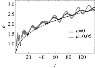
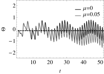
Figure 3. The evolution of $\rho(t)$ and $\Theta(t)=\varphi(t)-\varkappa^{-1}S(t)$ for sample paths of the resonant solutions $(\varkappa=1)$ to system (57) with $\mathcal{Q}=4$ and $s=1/2$. The black dashed curves correspond to $\rho(t)\equiv z_{0}t^{1/3}$ and $\Theta(t)\equiv\theta_{0}$, where $z_{0}\approx 0.56$, $\theta_{0}\approx-0.127$. In this case, $\mathcal{Q}_{1}\approx 2.04$.

2. Now let $p=n=1$, $\alpha=\beta=1/2$, and $\gamma=3/4$. Then, system (4) has the following form:

(58) $$dx_{1}=x_{2}\,dt,\quad dx_{2}=\left(x_{1}-x_{1}^{3}+t^{-\frac{1}{2}}\mathcal{Q}x_{1}\cos\left(st^{\frac{3}{2}}\right)\right)dt+t^{-\frac{3}{4}}\mu x_{1}\cos\left(st^{\frac{3}{2}}\right)\,dw(t).$$

We see that the inequalities (56) are satisfied. In this case, $a=b=-1$, $A=3/4$, $B=3/2$, $C=3/2$,

$$\mathcal{P}(\Theta) \equiv\frac{1}{\sqrt{6}}\left(\frac{2}{z_{0}}\langle f_{1,0}(\varkappa^{-1}\zeta+\Theta,\zeta)\rangle_{\varkappa\zeta}-1\right),$$

$$J(\Theta) \equiv\frac{2}{3z_{0}}\left\langle\partial_{\Theta}f_{2,0}(\varkappa^{-1}\zeta+\Theta,\zeta)\right\rangle_{\varkappa\zeta}+\frac{1}{6},$$

where

$$f_{1,0}(\varphi,S)\equiv\frac{\mathcal{Q}\nu_{0}}{8}\partial_{\varphi}(X_{1,0}(\varphi))^{2}\cos S,\quad f_{2,0}(\varphi,S)\equiv-\frac{\mathcal{Q}\nu_{0}}{4}(X_{1,0}(\varphi))^{2}\cos S,\quad z_{0}=\frac{3s}{2\nu_{0}\varkappa}.$$

In the case of a resonance with $\varkappa=2k$, $k\in\mathbb{Z}_{+}$, we have

(59) $$\mathcal{P}(\Theta)\equiv-\frac{1}{\sqrt{6}}\left(\frac{\mathcal{Q}}{s\mathcal{Q}_{k}}\sin(2k\Theta)+1\right),\quad J(\Theta)\equiv\frac{2\mathcal{Q}}{s\mathcal{Q}_{\varkappa}}\sin(2k\Theta)+\frac{1}{6},\quad\mathcal{Q}_{\varkappa}=\frac{3}{2(\nu_{0}k)^{2}\tilde{q}_{k}},$$

where $\tilde{q}_{k}=\langle(X_{1,0}(\zeta))^{2}\cos(2k\zeta)\rangle_{\zeta}$. It follows that if $|\mathcal{Q}|/s>\mathcal{Q}_{\varkappa}$, then the condition (26) holds with

$$\Theta_{0}\in\left\{(-1)^{j}\theta_{0}+\frac{\pi j}{2k}\right\}_{j\in\mathbb{Z}},\quad\theta_{0}=\frac{1}{2k}\arcsin\left(-\frac{s\mathcal{Q}_{\varkappa}}{\mathcal{Q}}\right).$$

It can easily be checked that for all $j\in\mathbb{Z}$

$$\mathcal{P}^{\prime}(\Theta_{0})=-\frac{(-1)^{j}2k\mathcal{Q}}{\sqrt{6}s\mathcal{Q}_{\varkappa}}\cos(2k\theta_{0})\neq 0,\quad J(\Theta_{0})=-\frac{1}{2}.$$

It follows from Lemma 3 and Theorem 2 that if $|\mathcal{Q}|/s>\mathcal{Q}_{\varkappa}$ and $(-1)^{j}\mathcal{Q}>0$, then a phase-locking regime occurs in system (58) such that

$$\rho(t)\approx\frac{3st^{\frac{1}{2}}}{4\nu_{0}k},\quad\varphi(t)\approx\frac{1}{2k}\left(S(t)+(-1)^{j}\arcsin\left(-\frac{s\mathcal{Q}_{\varkappa}}{\mathcal{Q}}\right)+\pi j\right),\quad k\in\mathbb{Z}_{+}.$$

Moreover, since $C=A+B/2$, we see that this mode is stochastically stable on the exponentially long time interval $t\leq\mathcal{O}(\exp\mu^{-4(1-\epsilon)/3})$ as $\mu\to 0$ for all $\epsilon\in(0,1)$ (see Fig. 4). If $|\mathcal{Q}|/s>\mathcal{Q}_{\varkappa}$ and $(-1)^{j}\mathcal{Q}<0$, this regime is unstable. The capture into resonance does not occur if $|\mathcal{Q}|/s<\mathcal{Q}_{\varkappa}$.

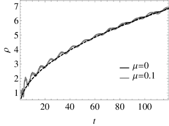
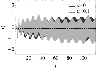
Figure 4. The evolution of $\rho(t)$ and $\Theta(t)=\varphi(t)-\varkappa^{-1}S(t)$ for sample paths of the resonant solutions $(\varkappa=2)$ to system (58) with $\mathcal{Q}=8$ and $s=1$. The black dashed curves correspond to $\rho(t)\equiv z_{0}t^{1/2}$ and $\Theta(t)\equiv\theta_{0}$, where $z_{0}\approx 0.63$, $\theta_{0}\approx-0.132$. In this case, $\mathcal{Q}_{2}\approx 2.101$.

3. Finally, let $p=1$, $n=2$, $\alpha=\beta=1/2$, and $\gamma=3/2$. Then, system (4) takes the form

(60) $$dx_{1}=x_{2}\,dt,\quad dx_{2}=\left(x_{1}-x_{1}^{3}+t^{-\frac{1}{2}}\mathcal{Q}x_{1}\cos\left(st^{\frac{3}{2}}\right)\right)dt+t^{-\frac{3}{2}}\mu x_{1}^{2}\cos\left(st^{\frac{3}{2}}\right)\,dw(t).$$

It can easily be checked that the inequalities (56) hold. It follows from (14), (24) and (25) that $a=b=0$, $A=3/4$, $B=3/2$, $C=7/4$. Note that in the case of $\varkappa=2k$, $k\in\mathbb{Z}_{+}$, the functions $\mathcal{P}(\Theta)$ and $J(\Theta)$ have the form (59). Thus, the results obtained for the previous example are valid. Moreover, since $C>A+B/2$, we obtain the stochastic stability of the resonance on an semi-infinite time interval if $|\mathcal{Q}|>\mathcal{Q}_{\varkappa}$ and $(-1)^{j}\mathcal{Q}>0$ (see Fig. 5).

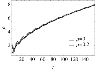
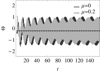
Figure 5. The evolution of $\rho(t)$ and $\Theta(t)=\varphi(t)-\varkappa^{-1}S(t)$ for sample paths of the resonant solutions $(\varkappa=2)$ to system (60) with $\mathcal{Q}=5$ and $s=1$. The black dashed curves correspond to $\rho(t)\equiv z_{0}t^{1/2}$ and $\Theta(t)\equiv\theta_{0}$, where $z_{0}\approx 0.63$, $\theta_{0}\approx-0.132$. In this case, $\mathcal{Q}_{2}\approx 2.101$.

9. Conclusion

Thus, the combined influence of a decaying chirped-frequency driving and a stochastic perturbation on the class of nonlinear systems far from the equilibrium have been investigated. Using a modified averaging method, we have derived the model truncated system (21), describing a possible dynamics in the perturbed system (1). We have shown that the model system has at least two regimes: phase locking and phase drifting. The resonant solutions with unlimitedly growing amplitude arise in the phase-locking mode. We have described the conditions that guarantee the persistent of such solutions in the full stochastic system on asymptotically large time intervals.

Note that the proposed technique cannot be applied directly to the case of more complicated limiting systems than (5). The same is true for multidimensional systems with chirped-frequency perturbations due to the small denominators that may appear when averaging the equations. These cases deserve special attention and will be discussed elsewhere.

References

- [1] S. Rajasekar, M. A. F. Sanjuán, Nonlinear Resonances, Springer, Switzerland. 2016.
- [2] L.I. Manevitch et al., Nonstationary Resonant Dynamics of Oscillatory Chains and Nanostructures, Springer-Verlag, Berlin, 2018.
- [3] L. Friedland, Autoresonance in nonlinear systems, Scholarpedia, 4 (2009), 5473.
- [4] G. Manfredi et al., Chirped-frequency excitation of gravitationally bound ultracold neutrons, Phys. Rev. D, 95 (2017), 025016.
- [5] L. Friedland et al., Excitation and control of large amplitude standing ion acoustic waves, Phys. Plasmas 26(2019), 092109.
- [6] L. A. Kalyakin, Asymptotic analysis of autoresonance models, Rus. Math. Surv., 63 (2008), 791–857.
- [7] O. M. Kiselev, Conditions for phase locking and dephasing of autoresonant pumping, Rus. J. Nonlin. Dyn., 15 (2019), 381–394.
- [8] A. Kovaleva, Autoresonance in weakly dissipative Klein-Gordon chains, Physica D, 402 (2020), 132284.
- [9] O. A. Sultanov, Autoresonance in oscillating systems with combined excitation and weak dissipation, Physica D, 417 (2021), 132835.
- [10] R. Bellman, Stability Theory of Differential Equations, McGraw-Hill, New York, 1953.
- [11] L. Markus, Asymptotically autonomous differential systems, Contributions to the Theory of Nonlinear Oscillations III, Ann. Math. Stud., 36, Princeton University Press, Princeton, 1956, 17–29.
- [12] L. D. Pustyl’nikov, Stable and oscillating motions in nonautonomous dynamical systems. A generalization of C. L. Siegel’s theorem to the nonautonomous case, Math. USSR-Sbornik, 23 (1974), 382–404.
- [13] H. Thieme, Asymptotically autonomous differential equations in the plane, Rocky Mountain J. Math., 24 (1994), 351–380.
- [14] O. A. Sultanov, Damped perturbations of systems with center-saddle bifurcation, Internat. J. Bifur. Chaos., 31 (2021), 2150137.
- [15] J. A. Langa, J. C. Robinson, A. Suárez, Stability, instability and bifurcation phenomena in nonautonomous differential equations, Nonlinearity, 15 (2002), 887–903.
- [16] P. E. Kloeden, S. Siegmund, Bifurcations and continuous transitions of attractors in autonomous and nonautonomous systems, Internat. J. Bifur. Chaos., 15 (2005), 743–762.
- [17] M. Rasmussen, Bifurcations of asymptotically autonomous differential equations, Set-Valued Anal., 16 (2008), 821–849.
- [18] O. A. Sultanov, Stability and bifurcation phenomena in asymptotically Hamiltonian systems, Nonlinearity, 35 (2022), 2513–2534.
- [19] O. A. Sultanov, Bifurcations in asymptotically autonomous Hamiltonian systems under oscillatory perturbations, Discrete & Continuous Dynamical Systems, 41 (2021), 5943–5978.
- [20] O. A. Sultanov, Decaying oscillatory perturbations of Hamiltonian systems in the plane, Journal of Mathematical Sciences, 257 (2021), 705–719.
- [21] P. N. Nesterov, Construction of the asymptotics of the solutions of the one-dimensional Schrödinger equation with rapidly oscillating potential, Math. Notes, 80 (2006), 233–243.
- [22] V. Burd, P. Nesterov, Parametric resonance in adiabatic oscillators, Results. Math., 58 (2010), 1–15.
- [23] O. A. Sultanov, Resonances in asymptotically autonomous systems with a decaying chirped-frequency excitation, Discrete and Continuous Dynamical Systems - B, 28 (2023), 1719–1749.
- [24] O. A. Sultanov, Capture into resonance in nonlinear oscillatory systems with decaying perturbations, J. Math. Sci. 262 (2022), 374–389.
- [25] M. I. Freidlin, A. D. Wentzell, Random Perturbations of Dynamical Systems, Springer-Verlag, New York, Heidelberg, Berlin, 1998.
- [26] J. A. D. Appleby, X. Mao, A. Rodkina, Stabilization and destabilization of nonlinear differential equations by noise, IEEE Trans. Autom. Control, 53 (2008), 683–691.
- [27] J. M. Seoane, M. A. F. Sanjuán, Escaping dynamics in the presence of dissipation and noise in scattering systems, Internat. J. Bifur. Chaos. 20 (2010), 2783–2793.
- [28] Y. Zheng, Q. Wang, C. Gan, Noise-induced pattern formation and synchronization in a square-lattice neuronal network, Internat. J. Bifur. Chaos., 22 (2012), 1250115.
- [29] I. Bashkirtseva, T. Ryazanova, L. Ryashko, Stochastic bifurcations caused by multiplicative noise in systems with hard excitement of auto-oscillations, Phys. Rev. E, 92 (2015), 042908.
- [30] J. A. D. Appleby, J. P. Gleeson, A. Rodkina, On asymptotic stability and instability with respect to a fading stochastic perturbation, Appl. Anal., 88 (2009), 579–603.
- [31] J. A. D. Appleby, J. Cheng, A. Rodkina, Characterisation of the asymptotic behaviour of scalar linear differential equations with respect to a fading stochastic perturbation, Discrete Contin. Dyn. Syst., Supplement (2011), 79–90.
- [32] O. I. Klesov, O. A. Tymoshenko, Unbounded solutions of stochastic differential equations with time-dependent coefficients, Annales Univ. Sci. Budapest., Sect. Comp., 41 (2013), 25–35.
- [33] O. A. Sultanov, Bifurcations in asymptotically autonomous Hamiltonian systems subject to multiplicative noise, Internat. J. Bifur. Chaos., 32 (2022), 2250164.
- [34] O. A. Sultanov, Long-term behaviour of asymptotically autonomous Hamiltonian systems with multiplicative noise, SIAM Journal on Applied Dynamical Systems, 22 (2023), 1818–1851.
- [35] M. V. Fedoryuk, Asymptotic methods in analysis, in Encyclopaedia of Mathematical Sciences, Analysis I (ed. R. V. Gamkrelidze), Springer, (1989), 83–191.
- [36] Øksendal, B. Stochastic Differential Equations. An Introduction with Applications, (Springer, New York, Heidelberg, Berlin).
- [37] N. N. Bogolubov, Yu. A. Mitropolsky, Asymptotic Methods in Theory of Non-linear Oscillations, Gordon and Breach, New York, 1961.
- [38] V. I. Arnold, V. V. Kozlov, A. I. Neishtadt, Mathematical Aspects of Classical and Celestial Mechanics, Springer, Berlin, 2006.
- [39] L. A. Kalyakin, Averaging method for the problems on asymptotics at infinity, Ufa Math. J., 1 (2009) 29–52.
- [40] O. A. Sultanov, Asymptotic analysis of systems with damped oscillatory perturbations, J. Math. Sci., 269 (2023), 111–128.
- [41] R. Khasminskii, Stochastic Stability of Differential Equations, Springer, Berlin, Heidelberg, 2012.
- [42] J. P. LaSalle, S. Lefschetz, Stability by Lyapunov’s Direct Method with Applications, Academic Press, New York, 1961.
- [43] H. J. Kushner, Stochastic Stability and Control, Academic Press, New York, 1967.
- [44] I. Kovacic et al., Jacobi elliptic functions: A review of nonlinear oscillatory application problems, J. Sound and Vibr., 380 (2016), 1–36.
- [45] N. I. Akhiezer, Elements of the Theory of Elliptic Functions, Translations of Mathematical Monographs, Amer. Math. Soc., Providence, 1990.